
Submitted:
24 January 2024
Posted:
24 January 2024
You are already at the latest version
Abstract
This paper presents a model for determining the availability of continuous systems at open pits using the neuro-fuzzy system. The concept of availability is divided into partial indicators (synthetic indicators and sub-indicators). The presented model in relation to already existing models for determining availability uses a combination of the advantages of artificial neural networks and fuzzy logic. The case study was done for the I ECC (bucket wheel excavator – conveyors – crushing plant) system of the open pit Drmno, Kostolac. In this paper, in addition to the ANFIS model for determining the availability of continuous systems, a simulation model was developed. The obtained results of the ANFIS model were verified with the help of a simulation model that uses certain assumptions about the distribution of failures. This paper was created as a result of several years of field and theoretical research into the availability of continuous sys-tems in open-pit mines, and completes a cycle that consists of several published articles on the subject of modeling the behavior of these systems in real time using a time picture of the state, expert assessment, simulation and AI models, respecting the multidisciplinarity of the problem (mining-technological, mechanical, information-technological aspects).
Keywords:
coal
; systems
; ECC system
; mining
; availability
; ANFIS
; simulation
1. Introduction
Surface exploitation of coal deposits is carried out in difficult and complex condi-tions. The operation of continuous systems and their availability is of great importance for the stability of the energy system of the Republic of Serbia, because the largest part of the coal needed for the operation of the power plant is obtained precisely by exploitation with continuous systems.
Continuous surface mining systems are systems where the flow of material is con-tinuous. They are characterized by excavation during the entire work cycle, in contrast to discontinuous ones, where only part of the time of one cycle is spent on excavation. The mechanization that is applied is very complex and made according to special require-ments, because these systems must be adapted to specific working conditions. The basic function of these systems when it comes to surface coal mine is to excavate, transport and deposit coal, which can be uniquely described as coal production.
2. Literature review
Models developed on the basis of neural networks and fuzzy logic are increasingly used in mining.
In the paper “Adaptive neuro-fuzzy prediction of operation of the bucket wheel drive based on wear of cutting elements” [1], Miletic et al. define an ANFIS model that aims to determine the dependence on how the wear of cutting elements affects the operation of the bucket wheel excavator.
In the paper “A Fuzzy Expert Model for Availability Evaluation” [2], Ivezic and others define the concept of availability of auxiliary machinery, bulldozers. The formed expert fuzzy model analyzes and integrates the partial indicators of the availability of bulldozers working at the surface mines (open pits) of the Electric Power Company of Serbia.
Petrović and others in the paper “Fuzzy Model for Risk Assessment of Machinery Failures” [3] present a model for the implementation of negative risk parameters in the synthetic risk assessment model of the Lokotrack LT 1213S mobile crusher operating at the open pit Ladna Voda. The model shows that there is a high level of risk and that it is necessary to introduce the concept of risk-based maintenance.
In the paper entitled “Applying the Fuzzy Inference Model in Maintenance Centered to Safety: Case Study - Bucket Wheel Excavator” Jovančić et al. [4] use the Fuzzy Inference Model to promote safety-centered maintenance, which has online adaptation to conditions work. The model was tested on a case study of two SRs 1200 and SchRs 630 bucket wheel excavators.
Gomilanovic M. and others in the paper entitled “Determining the Availability of Continuous Systems at Open Pits Applying Fuzzy Logic” [5] show a model for determining the availability of continuous systems at open pits using fuzzy logic (fuzzy inference system). The applied model was formed by the synthesis of independent partial indicators of availability. The model is based on an expert system for assessing the availability of continuous mining systems. System availability, as a complex state parameter, is decomposed into partial indicators, reliability and maintainability, and the fuzzy compositions used for the integration of partial indicators are max-min and min-max compositions.
Monjezi M. and others in the paper entitled “Evaluation of effect of blast design parameters on flyrock using artificial neural networks” [6] apply the method of artificial neural networks to predict the flying of fragments during blasting at the Sungun copper mine (Sungun), Iran. Several ANN (Artificial Neural Networks) models were run and it was observed that a model trained with a back propagation algorithm having a 9-5-2-1 architecture gives the best results. The flight of pieces was calculated side by side on the basis of available empirical models. Statistical modeling was also performed to compare the predictive ability of the artificial neural network against other methods. The comparison of the results showed the absolute superiority of the artificial neural network.
In the article of author Qin J. and others “SVNN-ANFIS approach for stability evaluation of open-pit mine slopes” [7], the analysis of the slope stability of open-pit mine slopes was performed using the ANFIS model with one value (SVNN-ANFIS). The stability of the surface mine slope has an important impact on the safe operation and economic benefits of the mining company. The results of applying the proposed methodology show that the accuracy of the training is 99.20%, while the accuracy of the testing process is 97.62%. This approach provides an innovative way to assess the slope stability of a surface mine.
The article “Predictive Model of Rock Fragmentation Using the Neuro-Fuzzy Inference System (ANFIS) and Particle Swarm Optimization (PSO) to Estimate Fragmentation Size in Open Pit Mining” [8] by Betty Vergara and others shows a predictive model to estimate rock fragmentation size using the ANFIS in combination with Particle Swarm Optimization (PSO). To build the predictive model, 92 blasting events were investigated and the rock fragmentation values were chosen, as well as three effective parameters on rock fragmentation, that is, burden, burden / spacing ratio, overdrilling and power factor. Based on statistical functions, correlation coefficient (R2) and mean square error (RMSE), it was found that the ANFIS-PSO model (with R2 = 0.85 and RMSE = 0.78) can be used as a reliable and acceptable model in the field prediction of rock fragmentation.
3. Case Study: I ECC System
The evaluation of the model in this article was performed on the continuous coal system (I ECC system) of the Drmno open pit, Kostolac.
The continuous coal system (I ECC system) of the Drmno Kostolac open pit consists of the following elements:
- Bucket wheel excavator SRs 400.14/1.5
- Beltwagon BRs 2400
- Belt conveyors
- Crushing plant
Figure 1.
Drmno open pit with the plotted position of the I ECC system (first photo photographed by the author of the article: M.G., second photo: source - Google Earth).
Figure 1.
Drmno open pit with the plotted position of the I ECC system (first photo photographed by the author of the article: M.G., second photo: source - Google Earth).
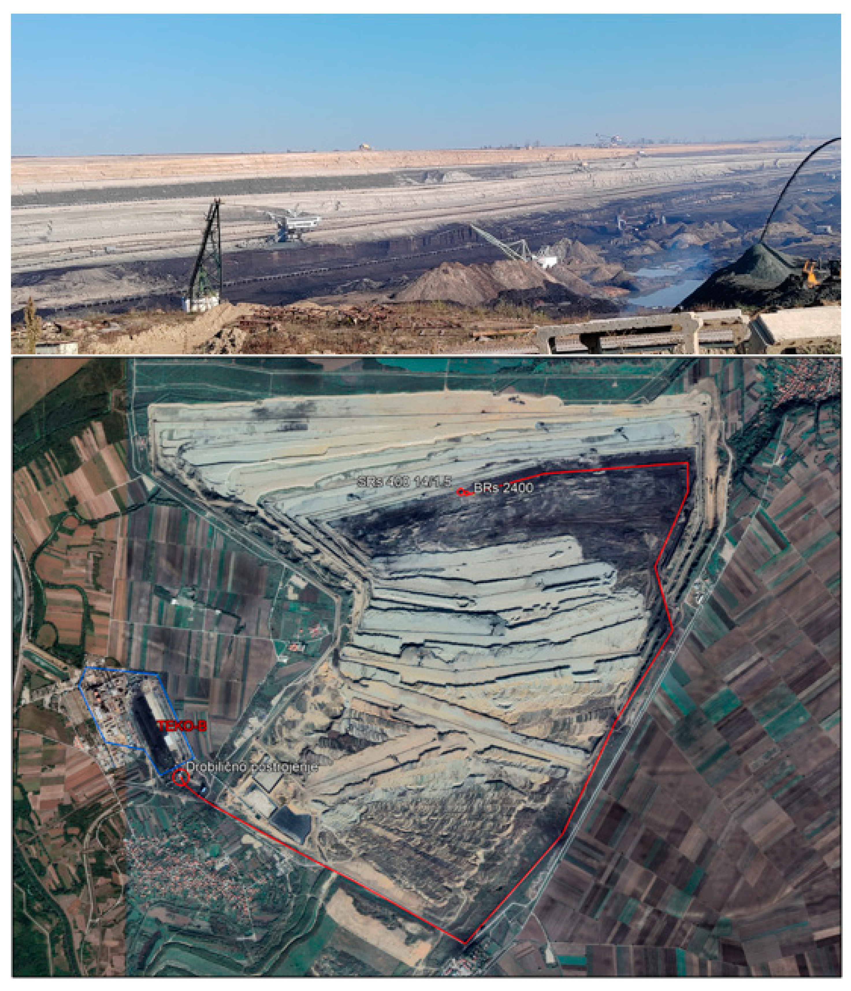
In Figure 2. a description of the equipment that makes up the I ECC system at the open pit Drmno Kostolac is given.
4. Availability
Availability represents the probability that the technical system will be able to work correctly at any moment in time, i.e., to start working and remain within the permitted deviations of the specified functions in a given time period and given working environment conditions”[11].
On the basis of the time state picture [12,13], where the times in the correct state alternate with the times in failure, the availability can be displayed and calculated [12,13]. The time when the technical system is operational (in working order) is divided into:
- time while the technical system waits to be put into operation () and
- time when the technical system is in operation ().
When the technical system is down, the time is divided into:
- organizational time (),
- logistic time () and
- active repair time () (time for corrective repairs () and time for preventive repairs ()).
5. Methods and material
5.1. Development of ANFIS model
The ANFIS model shown and described below was developed in the Python programming language, in the PyCharm 2023.2.1 editor. (Community Edition, Jet Brains) which is open user access.
ANFIS systems represent a synergy of artificial neural networks and fuzzy logic (fuzzy inference system). The advantage of these systems is reflected in the combination of using their positive features, namely the ability to learn with artificial neural networks and the use of expert knowledge with fuzzy logic.
The structure of the ANFIS system is similar to the structure of artificial neural networks, where based on the input-output set of data, a corresponding fuzzy inference system is formed and the parameters of the membership functions that transform the input data are calculated. The general structure of the ANFIS model consists of five layers (Figure 3). Below is a brief description of the layers.
In the first layer, the input data is transformed into a system of appropriate fuzzy sets. Accordingly, the output data of the first layer is determined by:
where is the input argument of the first layer, and is the membership function of the corresponding linguistic variable .
The second layer of the ANFIS model combines the output arguments of the different variables of the previous layer. The output data is determined by:
where and are two different variables.
The next layer includes the process of normalization of the values obtained in the second layer. The normalization process is carried out as follows:
The next layer is a layer that combines normalized values from the previous layer and first-order polynomials:
where , and are the parameters of the fourth layer model.
In the last layer, the normalized values of the previous layer are added using the following formula:
In Figure 4. the general architecture of the ANFIS model described in the previous part is shown.
Training of a neuro-fuzzy system is best done by applying a back-propagation process that uses the as the error function, which is defined by:
where , ,…, are actual values, and ,…, are values predicted by the ANFIS model.
When the input membership function parameters are set, the output from the ANFIS model is calculated as follows:
Using and , the following equality is obtained:
The process of training, i.e., model training, is based on the determination of parameter values, adjusted according to the training data. Back-propagation method is the basic way of training the system. This algorithm tries to minimize the error between the network and the desired output.
The determination of the availability of continuous systems and its partial indicators was processed through the results obtained through questionnaires related to the expert assessment of partial indicators of availability and to historical data on downtime and work, which include the time period from 2016 to 2019.
The availability of the ECC system is a function of the appropriate factors, which are most often divided into two groups - partial indicators, reliability and maintainability. These partial indicators (synthetic indicators) are further a function of a larger number of independent parameters (sub-indicators) that are considered as variables in this ANFIS model.
Figure 5.
Presentation of partial availability indicators [5] (synthetic indicators, sub-indicators).
Figure 5.
Presentation of partial availability indicators [5] (synthetic indicators, sub-indicators).
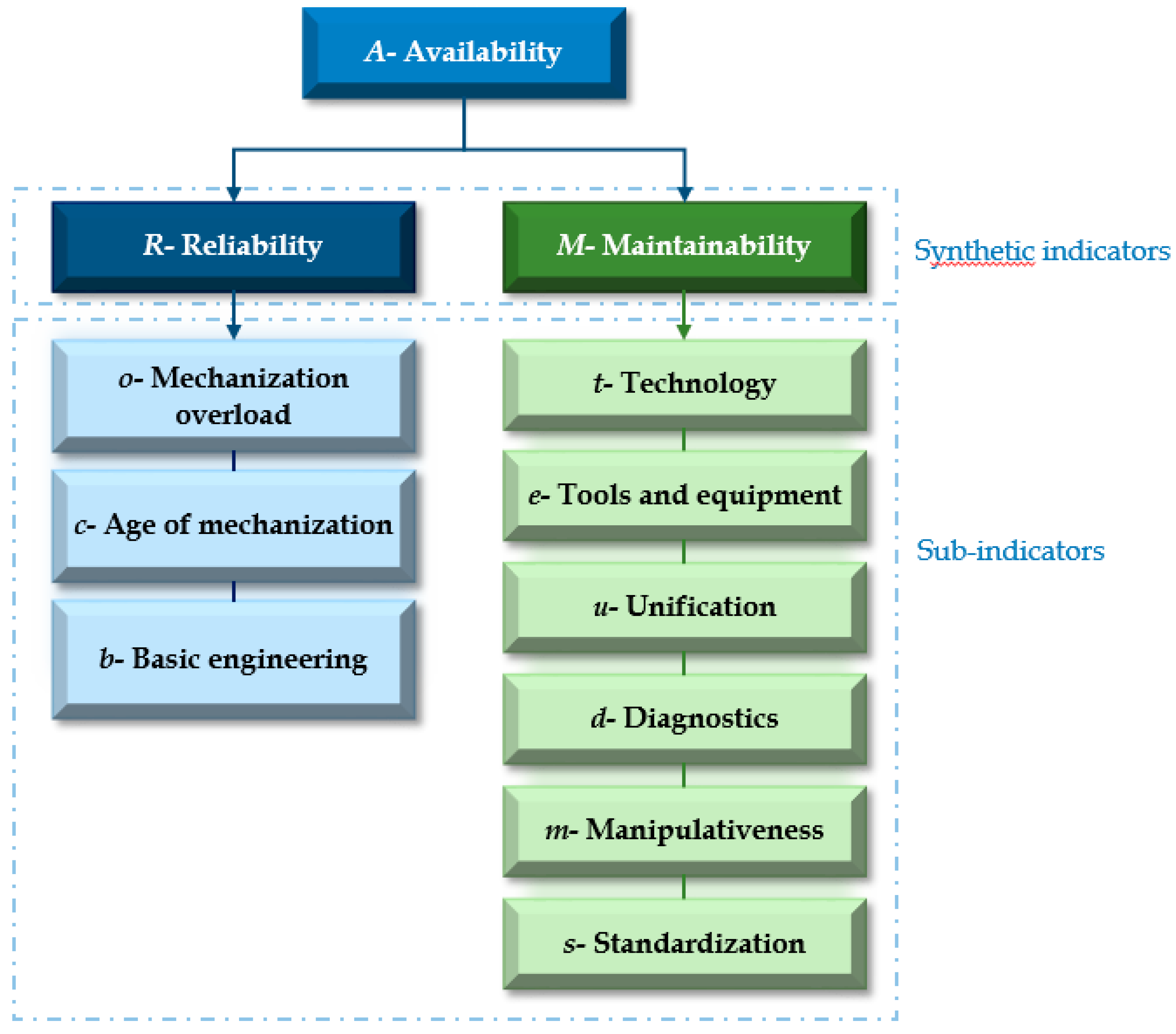
Within this model, availability decomposes into partial sub-indicators that are assessed by expert assessment, in the form of a questionnaire. Each part of the I ECC system (bucket wheel excavator, beltwagon, belt conveyors and crushing plant) is evaluated.
In the expert assessment, 10 experts from the field of continuous systems in surface exploitation were surveyed, who provided estimates for the sub-indicators of availability in a certain quarter and covering the period from 2016 to 2019 for each part of the ECC system. Data from 2016-2018 were used to train the ANFIS model (480 data - training data set), while data from 2019 (160 data - test data set) were used to test the obtained model. The experts were offered grades in the questionnaire ranging from (the worst grade) to (the best grade). The layout of the questionnaire is shown in Figure 6, with the fact that in this questionnaire the expert is required to make assessments at the quarterly level in a predetermined period of time for each part I of the ECC system. The scores obtained in this way were used as input data of this model.
Before creating the model, a database was created related to the duration of mechanical, electrical and other failures of the ECC system over a period of 4 years (2016, 2017, 2018, 2019). Data from this database is used to determine historical availability on a quarterly basis, and as such is used as output data of the ANFIS model. Availability per quarter was calculated based on the formula (1.).
In Table 1. part of the database is shown. The data was taken from the Electric Power Company of Serbia and contained information about downtimes on the specific system in the specified time period.
Based on the available data, the availability of the system was determined quarterly and the obtained values are shown in Table 2.
The resulting ANFIS model received the survey results for all 9 partial sub-indicators for each part of the I ECC system as input parameters, while the output represented the corresponding availability in the quarter to which the survey results refer, which was obtained based on historical data taken from the Electric Power Company of Serbia.
In the first step of the model, fuzzification was performed, which represents the transformation of partial indicator scores, using membership functions, into the corresponding -scale for =10. Predefined fuzzy sets are not used for probability functions, but membership functions are used instead, the parameters of which are estimated within the model training process. The membership functions used are Bell-shaped membership function, Gaussian membership function and Sigmoid membership function.
Using IF-THEN rules that are pre-defined, the synthetic indicator is determined based on the partial sub-indicators , , and the synthetic indicator is determined based on the partial sub-indicators , , , , , .
In the following, we will illustrate the determination of the synthesis indicator using IF-THEN rules based on sub-indicators , , . Let the IF-THEN rule be defined by IF AND AND THEN where i,j,k are in the set {}, and is in the set {}. Then the fuzzy sets come together:
where , and are the input values of grades ,, respectively for partial indicators , , , assigns the value . The fuzzy set corresponding to the rating of the indicator is the sum of all fuzzy sets assigned the value . In a similar way, on the basis of sub-indicators , , , , , , the synthesis indicator is calculated.
In the next step, using the IF-THEN rules, as described in the previous paragraph, the availability indicator is determined by synthetic indicators and . Then, the Euclidean distance of the obtained fuzzy sets from the fuzzy sets assigned to the availability indicator is determined based on the corresponding membership functions whose parameters we estimate within this ANFIS model. The distances ,, , and determined in this way can be joined by the normalized reciprocal values of the relative distances determined by:
These values represent belonging to the appropriate set of grades that determine the indicator of availability, i.e.,
Finally, the linguistic description is transformed into a numerical designation:
Dividing by 5 gives the predicted value of availability, which is compared with the realized value of availability calculated on a quarterly basis.
The IF-THEN rules used in this ANFIS model are shown in the following tables. So, for example, the values shown in the first type of this table are interpreted as follows:
If the partial sub-indicator is (the conditions of the working environment are such that the engaged equipment generally does not meet them) and if the partial sub-indicator is (write-off machine, very high level of failure) and if the partial sub-indicator is (underdeveloped basic engineering) then indicator is unreliable .

Table 3.
IF-THEN rules for determining the indicator - reliability
| F | F | F | E |
| E | E | E | D |
| D | D | D | C |
| C | C | C | B |
| B | B | B | A |
| B | C | B | A |
| C | B | C | B |
| C | B | B | A |
| B | C | D | B |
| C | C | B | B |
| D | C | D | C |
| E | B | E | C |
| C | D | B | A |
| E | E | D | D |
| C | C | A | A |
| D | C | B | B |
| B | B | A | A |
| B | C | D | B |
| A | B | A | A |
| D | B | B | A |
| D | E | A | B |
| A | C | C | A |
| A | C | D | B |
| A | B | B | A |
| A | E | D | B |
| A | B | C | A |
| B | C | E | B |
| B | D | D | B |
| B | E | E | C |
| B | B | A | A |
| A | A | A | A |
| F | E | E | D |
| F | D | D | C |
| F | C | C | B |
| F | A | A | A |
| F | E | D | D |
| E | D | C | C |
| D | C | B | B |
| C | B | A | A |
Table 4.
IF-THEN rules for determining the indicator – maintainability
| F | F | F | F | F | F | E |
| E | E | E | E | E | E | D |
| D | C | C | C | B | B | B |
| D | C | C | C | C | C | B |
| D | C | A | C | B | B | A |
| C | B | B | B | C | B | A |
| B | C | B | B | B | B | A |
| B | D | D | C | C | C | B |
| C | C | D | B | B | B | B |
| D | C | D | C | D | B | B |
| E | D | C | B | B | C | B |
| C | B | B | B | B | B | A |
| B | D | C | C | B | B | B |
| C | C | B | B | D | C | B |
| B | B | B | B | B | A | A |
| B | A | C | C | C | B | A |
| C | C | B | C | B | B | A |
| C | C | C | C | B | B | B |
| C | D | C | C | D | C | B |
| C | C | B | B | C | D | B |
| C | A | B | C | D | C | B |
| B | C | D | D | D | B | B |
| D | D | D | D | D | D | C |
| C | C | C | C | C | C | B |
| B | B | B | B | B | B | A |
| A | A | A | A | A | A | A |
| E | E | E | D | D | D | C |
| D | D | D | C | C | C | B |
| C | C | C | B | B | B | A |
| B | B | B | A | A | A | A |
| F | E | D | C | B | A | B |
| E | E | D | C | B | A | B |
| D | E | D | C | B | A | B |
| C | E | D | C | B | A | B |
| B | E | D | C | B | A | A |
| A | E | D | C | B | A | A |
Table 5.
IF-THEN rules for determining - availability
| D | D | D |
| D | C | C |
| D | B | C |
| D | A | B |
| C | D | C |
| B | D | C |
| C | C | C |
| B | B | B |
| A | A | A |
| E | D | D |
| C | B | B |
| B | A | A |
| C | A | B |
A summary of the considered models for predicting availability is given in Table 6.
5.2. Development of Simulation model
During the creation of the simulation model, all failures were classified into one of three types of failure (mechanical, electrical, and others). As in the case of the ANFIS model, the simulation model was developed based on data from three years (2016., 2017. and 2018. year).
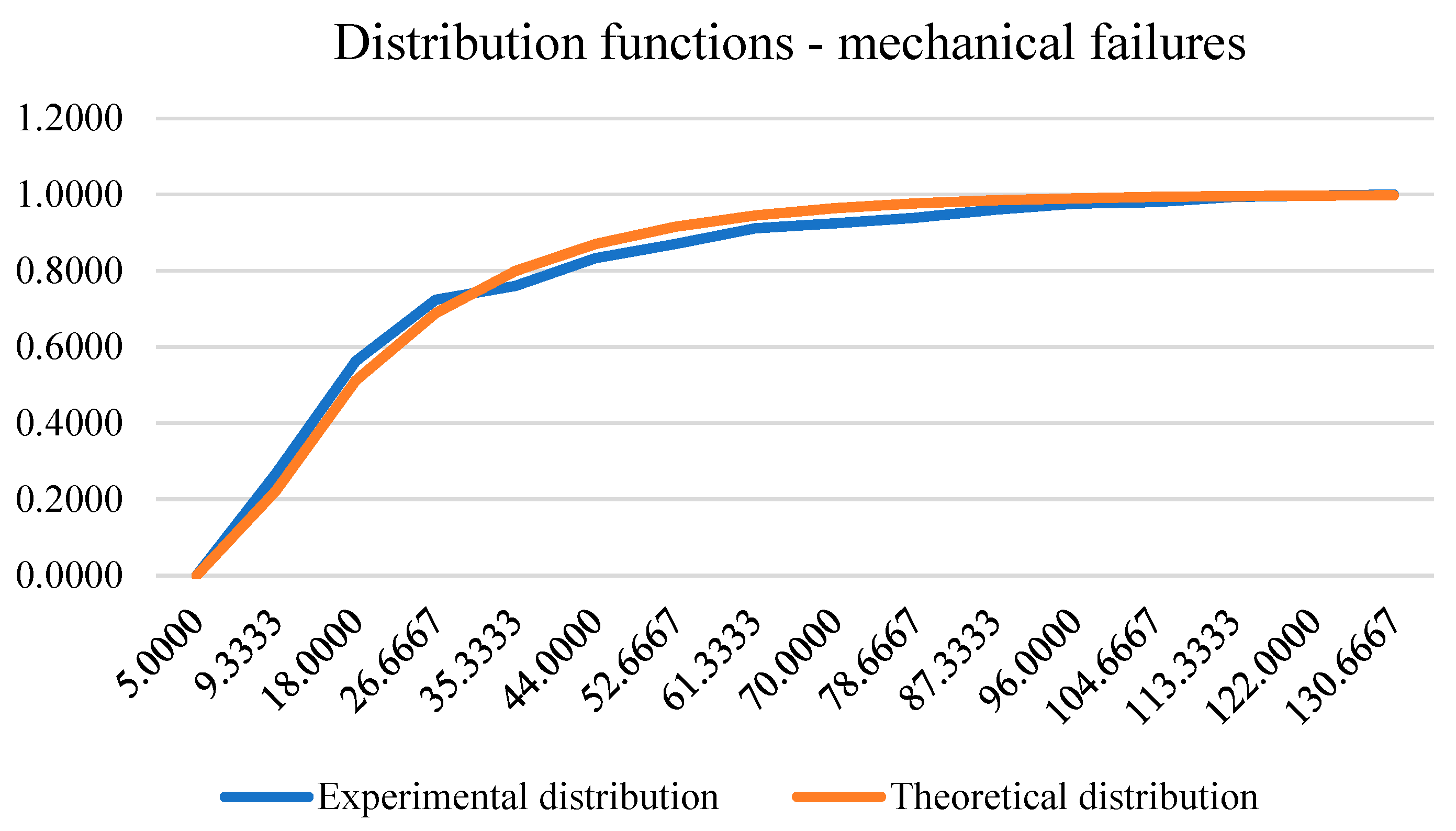
In Table 7. experimental and theoretical frequencies of machine failures by intervals are given.
The distribution of mechanical failure times, which was considered in the 96 percentile of the data, conforms to the Weibull distribution with parameters , i . More precisely, the empirical distribution function is determined by:
The number of mechanical failures on which this model was developed amounted to 1238 failures. The testing of the hypothesis about the distribution of data was performed with the help of the Kolmogornov-Smirnov test whose statistic value is equal to 1.7944, so with a significance level of 0.001 we cannot reject the null hypothesis that claims that the data are in accordance with the Weibull distribution. The following figure shows the experimental and theoretical function of the distribution of mechanical failures.
Figure 7.
Experimental and theoretical distribution function of mechanical failures.
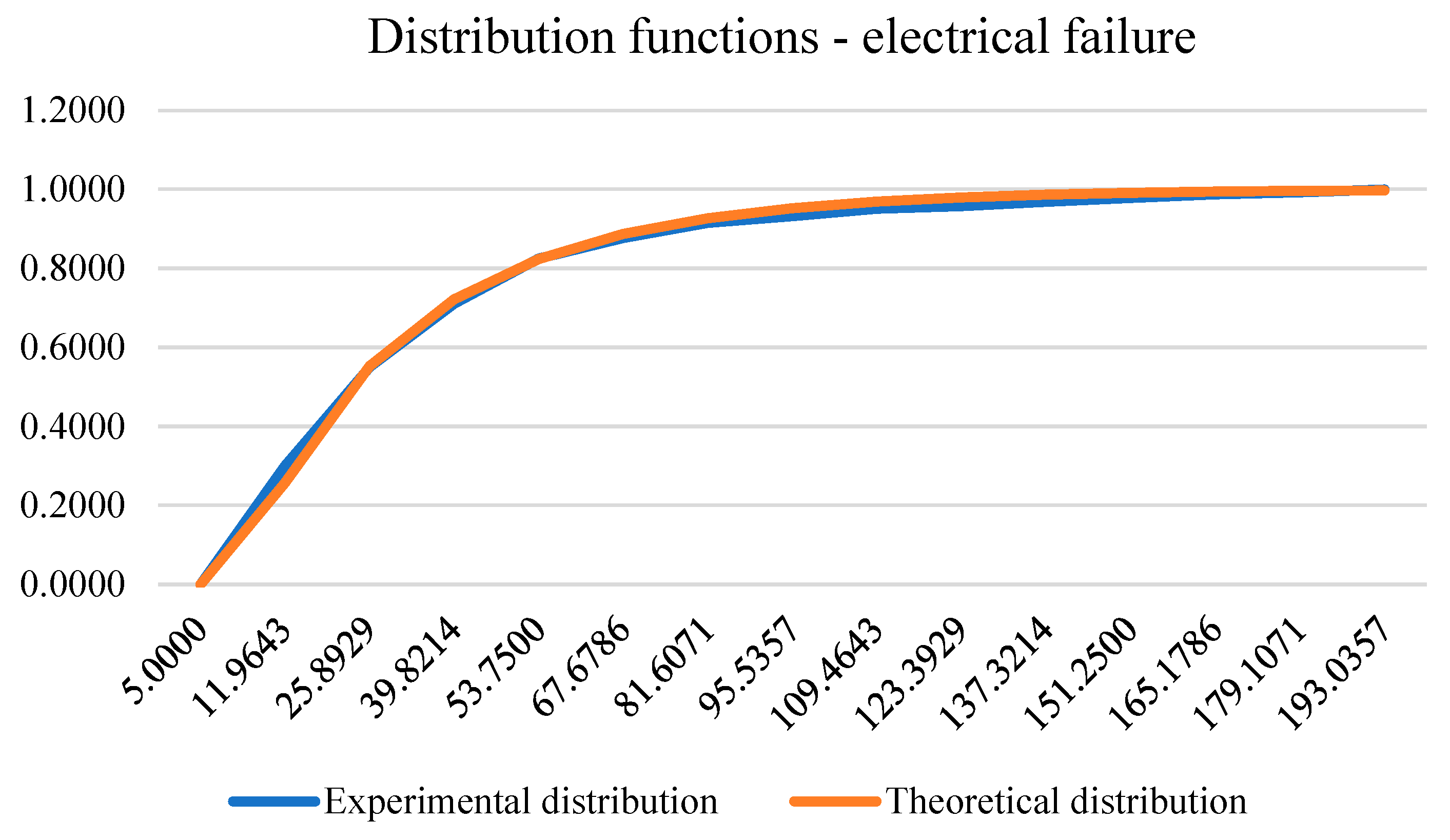
In Table 8. experimental and theoretical frequencies of electrical failures by intervals are given.
The distribution of the duration of electrical failure, which was considered in the 98.5 percentile of the data, is in accordance with the Weibull distribution with parameters , and . More precisely, the empirical distribution function is determined by:
The number of electrical failures on which this model was developed amounted to 908 failures. Testing of the hypothesis about data distribution was performed with the help of the Kolmogornov-Smirnov test whose statistic value is equal to 1.2804, so with a significance level of 0.05 we cannot reject the null hypothesis which claims that the data are in accordance with the Weibull distribution. The following figure shows the experimental and theoretical distribution function of electrical failure.
Figure 8.
Experimental and theoretical distribution function of electrical failure.
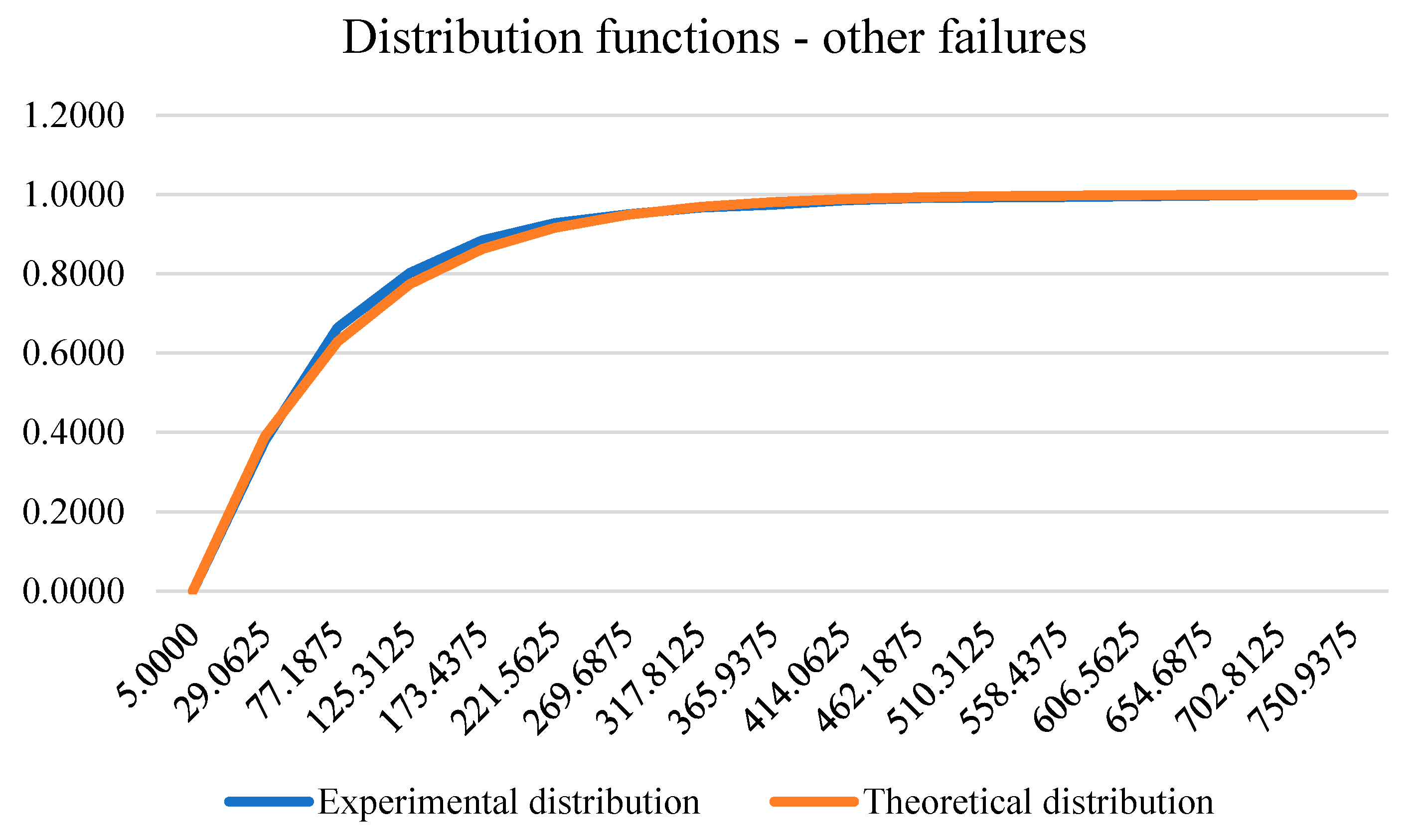
In Table 9. experimental and theoretical frequencies of other failures by intervals are given.
Table 9.
Experimental and theoretical frequency of other failures by intervals.
| No. | The lower bound of the interval | The upper bound of the interval | Experimental pdf | Experimental cdf | Theoretical pdf | Theoretical cdf | KS test |
| 1 | 5 | 53 | 0.3803 | 0.3803 | 0.3910 | 0.3910 | 0.0107 |
| 2 | 53 | 101 | 0.2837 | 0.6640 | 0.2381 | 0.6291 | 0.0350 |
| 3 | 101 | 149 | 0.1384 | 0.8025 | 0.1450 | 0.7741 | 0.0284 |
| 4 | 149 | 198 | 0.0823 | 0.8847 | 0.0883 | 0.8624 | 0.0223 |
| 5 | 198 | 246 | 0.0433 | 0.9281 | 0.0538 | 0.9162 | 0.0119 |
| 6 | 246 | 294 | 0.0217 | 0.9498 | 0.0328 | 0.9490 | 0.0008 |
| 7 | 294 | 342 | 0.0172 | 0.9670 | 0.0200 | 0.9689 | 0.0019 |
| 8 | 342 | 390 | 0.0069 | 0.9739 | 0.0122 | 0.9811 | 0.0072 |
| 9 | 390 | 438 | 0.0113 | 0.9852 | 0.0074 | 0.9885 | 0.0032 |
| 10 | 438 | 486 | 0.0054 | 0.9906 | 0.0045 | 0.9930 | 0.0023 |
| 11 | 486 | 534 | 0.0015 | 0.9921 | 0.0027 | 0.9957 | 0.0036 |
| 12 | 534 | 583 | 0.0015 | 0.9936 | 0.0017 | 0.9974 | 0.0038 |
| 13 | 583 | 631 | 0.0015 | 0.9951 | 0.0010 | 0.9984 | 0.0033 |
| 14 | 631 | 679 | 0.0020 | 0.9970 | 0.0006 | 0.9990 | 0.0020 |
| 15 | 679 | 727 | 0.0020 | 0.9990 | 0.0004 | 0.9994 | 0.0004 |
| 16 | 727 | 775 | 0.0010 | 1.0000 | 0.0002 | 0.9996 | 0.0004 |
The distribution of the duration of other failures, which was considered in the 100 percentile of the data, is in accordance with the exponential distribution with parameters , . More precisely, the empirical distribution function is determined by:
The number of other failures on which this model was developed amounted to 2030 failures. The testing of the hypothesis about the data distribution was performed with the help of the Kolmogornov-Smirnov test whose value of the statistic is equal to 1.5761, so with a significance level of 0.01 we cannot reject the null hypothesis which claims that the data are in accordance with the exponential distribution. The following figure shows the experimental and theoretical distribution function of other failures.
Figure 9.
Experimental and theoretical distribution function of other failures.
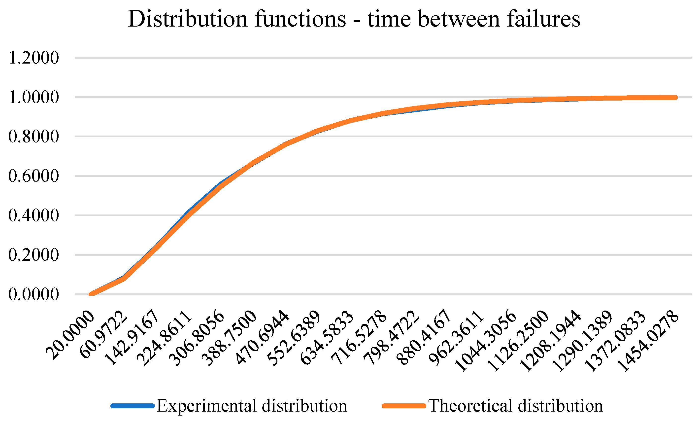
In Table 10. the presentation of experimental and theoretical frequencies of duration between failures by intervals is given.
The distribution of the duration between failures, which was considered in the 95 percentile of the data, is in accordance with the Erlang distribution with parameters , and . More precisely, the empirical distribution function is determined by:
The number of times between failures on which this model was developed was 5212. The testing of the hypothesis about the distribution of data was carried out with the help of the Kolmogornov-Smirnov test whose value of the statistic is equal to 1.0192, so with a significance level of 0.2 we cannot reject the null hypothesis that claims that are data in accordance with the Erlang distribution. The following figure shows the experimental and theoretical time distribution function between failures.
Figure 10.
Experimental and theoretical time distribution function between failures.
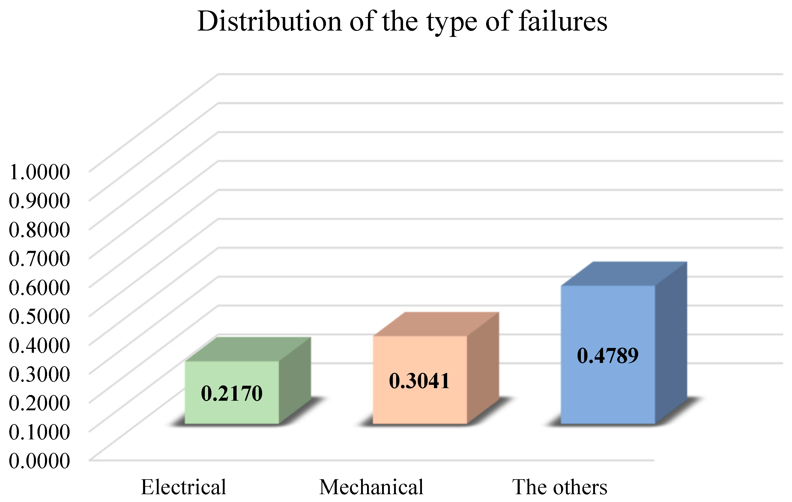
The following figure shows the frequency distributions of the considered failure types.
Figure 11.
Frequency distribution of the considered failure types.
The simulation model, whose algorithm is shown in the following figure (Figure 12), based on a randomly selected number from the distribution of the type of failure, generates a type of failure, and based on the next randomly selected number, the length of the failure of the selected type of failure is generated based on the distribution functions described above. Then, based on the new randomly selected number and the time-between-failure distribution function, the duration between failures is generated.
Glossary
tsim – duration of the simulation (s),
Nosim – number of simulations,
State – state ECC system: 1 – „working time“; 0 – „downtime“,
rnumber – random number generated by uniform distribution in the interval [0...1],
cs- current simulation,
tsim – simulation time,
TBF – time between failures (current),
DT – downtime failures (current),
tef – failure completion time (in simulation),
tbf – failure start time (in simulation),
VRflr – type of failure: 1 - mechanical; 2 – electrical; 3- other,
AECC – system availability - ECC,
A (t) – availability of the system at a given time t,
ka – stationary availability value.
6. Conclusion
Based on the displayed values of statistics shown in table 6 the conclusion is reached that the model, which uses a Gaussian function to determine affiliation, has a better prediction ability compared to other models, which use sigmoid or bell-shaped function to determine affiliation memebership function.
Using the obtained ANFIS model and the scores of partial sub-indicators provided by the experts for the next time period, the prediction of availability is obtained, which amounts to: 0.8090 that is 81%. Based on the simulation model, the availability value is 0.8513, i.e., 85%. Bearing in mind that the average availability in the time period of three years that was considered within the training of ANFIS and the simulation model is equal to 0.8132, i.e., 81%, while the value of availability for the year 2019 is 0.7797, i.e., 78%, we conclude that the ANFIS model gives a closer picture of the state of availability I ECC system. An additional advantage of this model is its simplicity, which does not include certain assumptions about data distribution. Figure 13 shows the obtained availability values.
The assessment of availability using the ANFIS model is necessary information for production planning in surface mines with continuous systems. The obtained availability value represents a limitation regarding the realization of coal mining, transport and storage capacity and defines the need for possible interventions regarding its increase if there is a demand for it from the aspect of realization of the projected/required capacity.
Author Contributions
Conceptualization, M.G. and U.B.; methodology, (ANFIS model) M.G. and (simulation model) U.B.; Writing –review and editing M.G., M.B., S.S. and N.S., supervision M.B., N.S. and S.S. All authors have read and agreed to the published version of the manuscript.
Funding
This work was financially supported by the Ministry of Education, Science and Technological Development of the Republic of Serbia, Grant No. 451-03-47/2023-01/ 200052 and Mining and Metallurgy Institute Bor.
Acknowledgments
Gratitude to the Ministry of Education, Science and Technological Development of the Republic of Serbia. Mining and Metallurgy Institute Bor, Zeleni bulevar 35, Bor. PE Electric Power Industry of Serbia, Balkanska 13, 11000 Belgrade. PE Electric Power Industry of Serbia - Branch “TE-KO Kostolac”, Nikola Tesla 5-7, 12208 Kostolac. Ministry of mining and energy Republic of Serbia, Nemanjina 22-26, Belgrade
Conflicts of Interest
The authors declare no conflict of interest.
References
- Miletic, F., Jovancic, P., Milovancevic, M., Ignjatovic, D., Adaptive neuro-fuzzy prediction of operation of the bucket wheel drive based on wear of cutting elements, Advances in Engineering Software, vol. 146, 2020, 102824, pp. 7-12. [CrossRef]
- Ivezic, D., Tanasijevic, M., Jovancic, P. and Đuric, R., A Fuzzy Expert Model for Availability Evaluation, 2019 20th International Carpathian Control Conference (ICCC), 2019, pp. 1-6. [CrossRef]
- Petrovic, D.,Tanasijevic, M., Stojadinovic, S., Ivaz, J. and Stojkovic, P., Fuzzy Model for Risk Assessment of Machinery Failures, Symmetry, MDPI, Basel, 2020, 12(4), 525. [CrossRef]
- Jovancic, P., Tanasijevic, M., Milisavljevic, V., Cvjetic, A., Ivezic, D. and Bugaric, U., Applying the Fuzzy Inference Model in Maintenance Centered to Safety: Case Study – Bucket Wheel Excavator, Applications and Challenges of Maintenance and Safety Engineering in Industry 4.0, IGI Global, 2020, pp. 142-165. [CrossRef]
- Gomilanovic, M., Tanasijevic, M. and Stepanovic ,S., Determining the Availability of Continuous Systems at Open Pits Applying Fuzzy Logic, Energies, 2022, 15(18):6786. [CrossRef]
- Monjezi, M., Mehrdanesh, A., Malek, A., and Khandelwal, M., Evaluation of effect of blast design parameters on flyrock using artificial neural networks, Neural Computing and Applications, vol. 23, no. 2, 2013, pp. 349-356. [CrossRef]
- Qin, J.; Du, S.; Ye, J.; & Yong R. (2022) SVNN-ANFIS approach for stability evaluation of open-pit mine slopes. Expert Systems with Applications 198:116816. [CrossRef]
- Vergara, B., Torres, M., Aramburu, V., Raymundo, C. (2021). Predictive Model of Rock Fragmentation Using the Neuro-Fuzzy Inference System (ANFIS) and Particle Swarm Optimization (PSO) to Estimate Fragmentation Size in Open Pit Mining. In: Trzcielinski, S., Mrugalska, B., Karwowski, W., Rossi, E., Di Nicolantonio, M. (eds) Advances in Manufacturing, Production Management and Process Control. AHFE 2021. Lecture Notes in Networks and Systems, vol 274. Springer, Cham. [CrossRef]
- Bugaric, U., Tanasijevic, M., Gomilanović, M., Petrović, A., Ilić, M., Analytic determination of the availability of a rotary excavator as a part of coal mining system-Case study: Rotary excavator SchRs 800.15/1,5 of the Drmno open pit, Mining and Metallurgy Engineering Bor, 3-4, 2020, Bor (2020), ISSN 2406-1395, UDC 622.
- Gomilanovic, M., Stanic, N., Milijanovic, D., Stepanovic, S., Milijanovic, A., Predicting the availability of continuous mining systems using LSTM neural network, Advances in Mechanical Engineering, vol. 14, issue 2, 2022. [CrossRef]
- Bugaric, U., Petrovic, D., Modeling of service systems, Faculty of Mechanical Engineering, Belgrade, University of Belgrade, 2011 year, ISBN: 978-86-7083-749-2.
- Djenadic, S., Ignjatovic, D., Tanasijevic, M., and others, Development of the Availability Concept by Using Fuzzy Theory with AHP Correction, a Case Study: Bulldozers in the Open-Pit Lignite Mine, 2019, Energies, MDPI, 12(21), 4044. [CrossRef]
- Gomilanovic, M.; Tanasijevic, M.; Stepanovic, S.; Miletic, F. A Model for Determining Fuzzy Evaluations of Partial Indicators of Availability for High-Capacity Continuous Systems at Coal Open Pits Using a Neuro-Fuzzy Inference System. Energies 2023, 16, 2958. [CrossRef]
- Milovancevic M, Cirkovic B, Denic N, Paunovic M, Prediction of Shear Debonding Strength of Concrete Structure with High- 312 Performance Fiber Reinforced Concrete, Structures 33(5-6):4475-4480. [CrossRef]
Figure 2.
I ECC system at the open pit Drmno, Kostolac (photographed by the author of the article: M.G.).
Figure 2.
I ECC system at the open pit Drmno, Kostolac (photographed by the author of the article: M.G.).
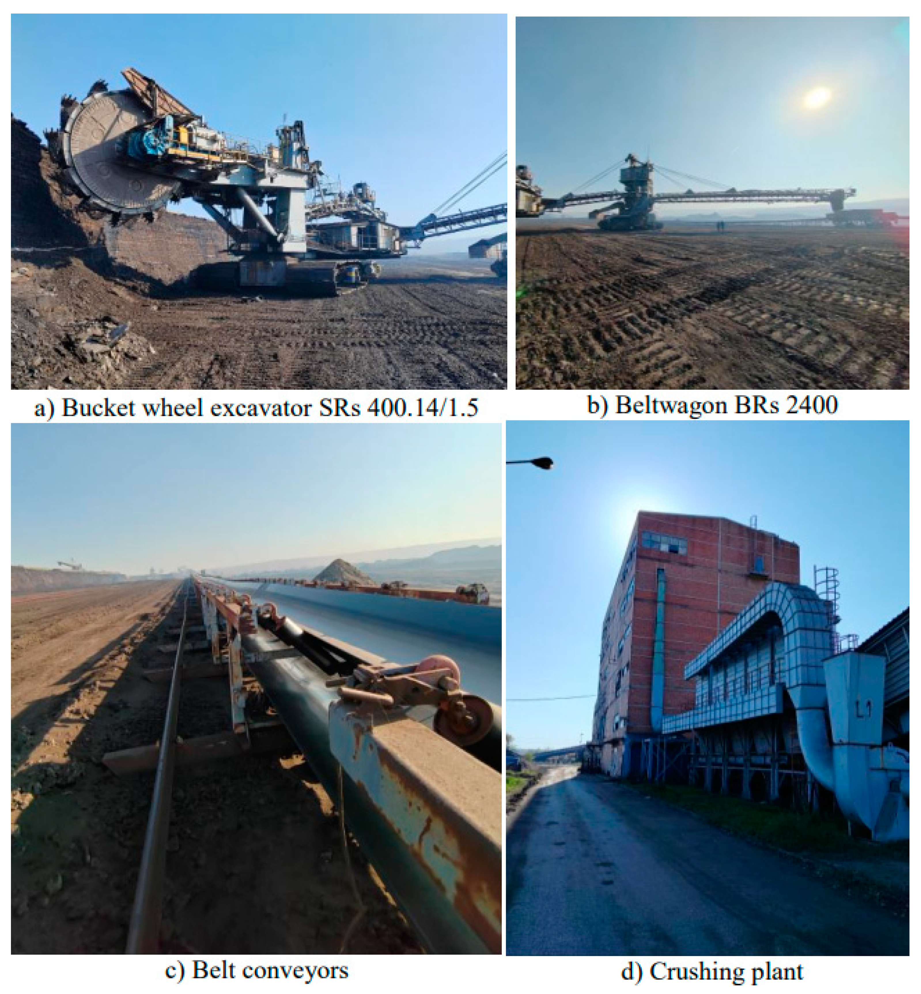
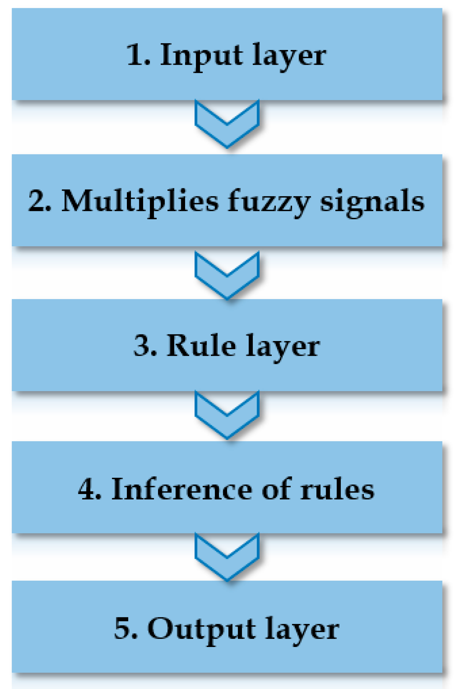
Figure 4.
ANFIS model architecture [13].
Figure 4.
ANFIS model architecture [13].
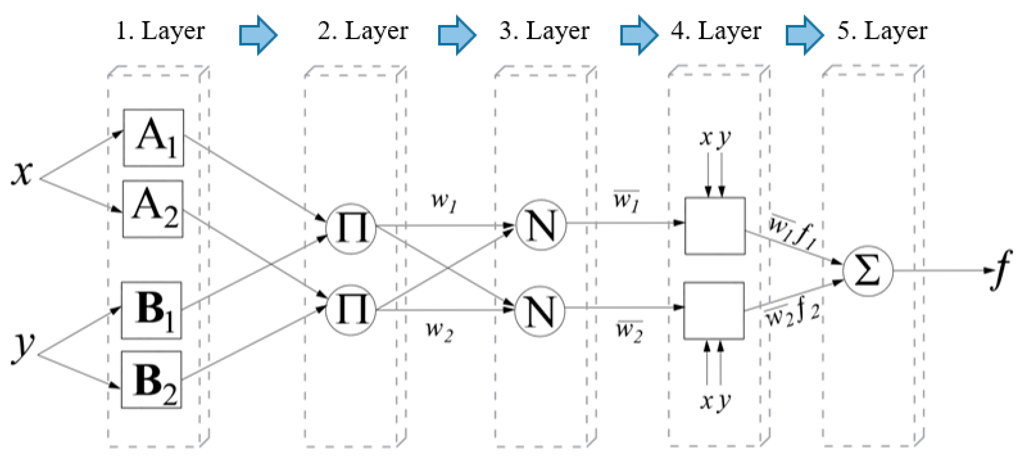
Figure 6.
Layout of the questionnaire.

Figure 12.
Algorithm of the simulation model.
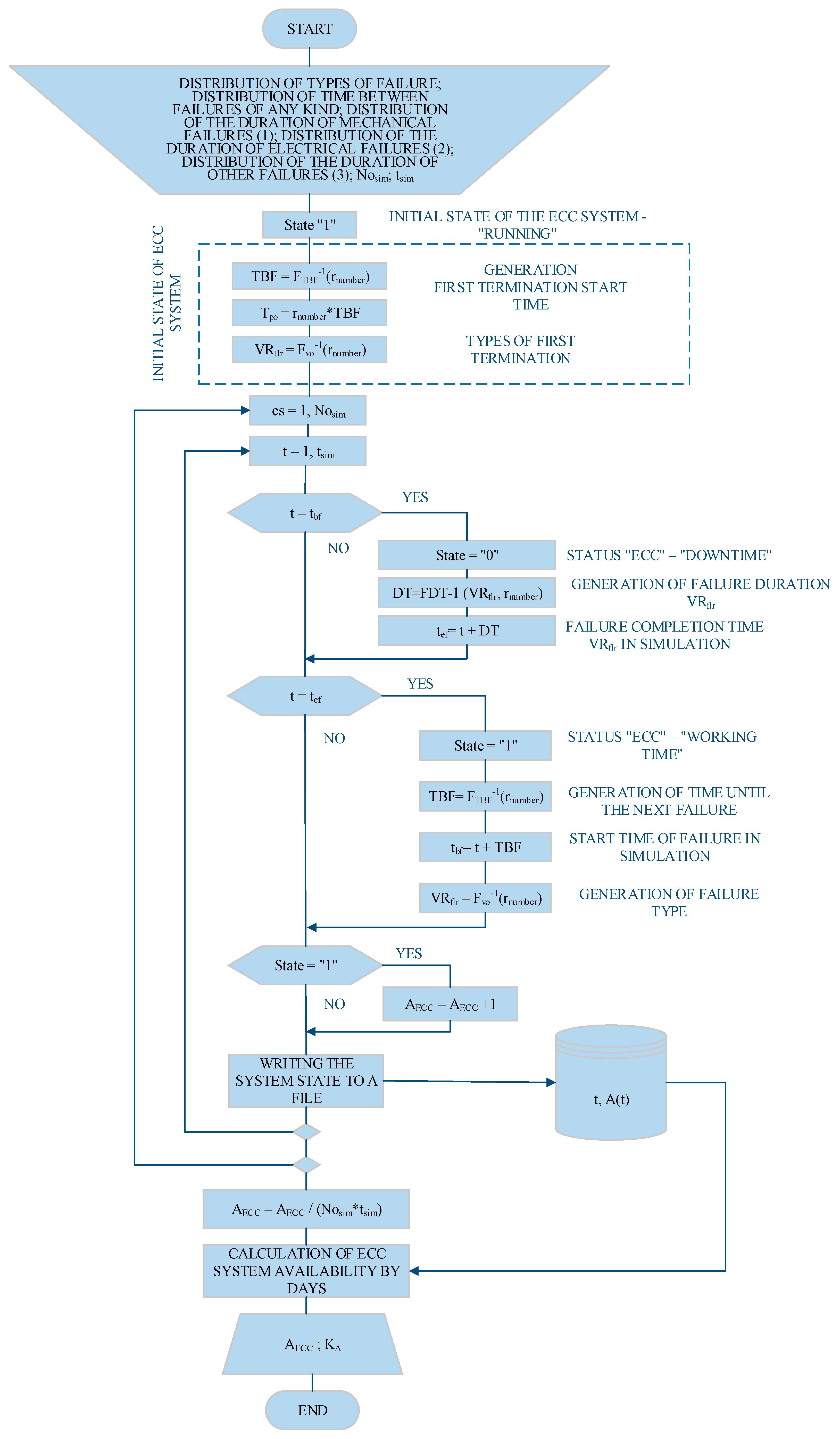
Figure 13.
Display of obtained availability values.
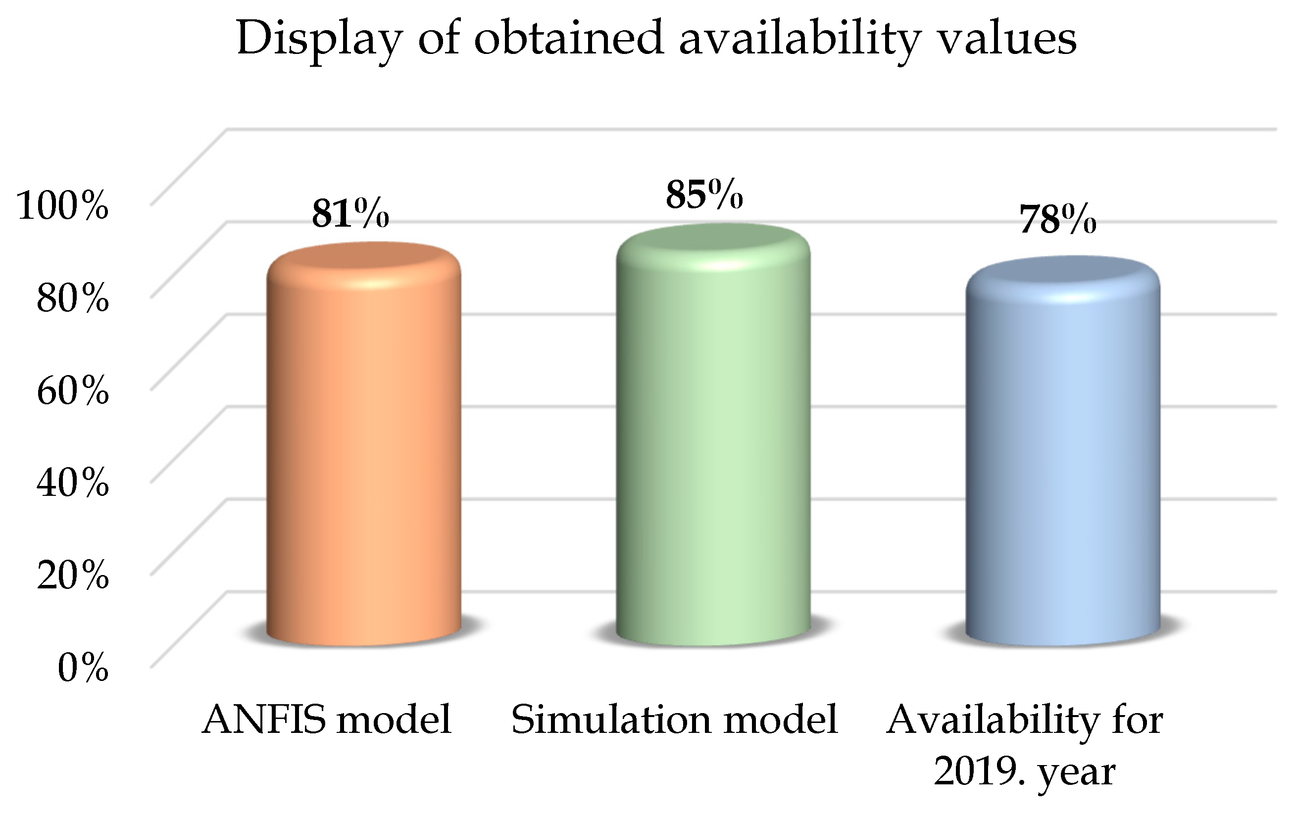
Table 1.
Presentation of part of the database on downtimes of the I ECC system.
| Date | Month | Year | System | Object | Failure | Start offailure | The end of failure | Downtime | Total downtime (min.) | Note | Shift |
| 1.1.2016 | January | 2016 | I ECC | BWE SRs-400 | Electrical | 10:00:00 | 10:50:00 | 00:50 | 50 | / | 1 |
| 1.1.2016 | January | 2016 | I ECC | Crush. plant | Other | 13:00:00 | 14:30:00 | 01:30 | 90 | / | 1 |
| 1.1.2016 | January | 2016 | I ECC | BWE SRs-400 | Electrical | 19:00:00 | 19:10:00 | 00:10 | 10 | / | 2 |
Table 2.
Obtained results for the availability of the I ECC system.
| Year | Quarter | Availability | Year | Quarter | Availability |
| 2016 | 1 | 0.8300 | 2018 | 1 | 0.8039 |
| 2 | 0.8203 | 2 | 0.8425 | ||
| 3 | 0.8018 | 3 | 08365 | ||
| 4 | 0.8008 | 4 | 0.7790 | ||
| Year | Quarter | Availability | Year | Quarter | Availability |
| 2017 | 1 | 0.8079 | 2019 | 1 | 0.8100 |
| 2 | 0.7825 | 2 | 0.7500 | ||
| 3 | 0.8370 | 3 | 0.7831 | ||
| 4 | 0.8177 | 4 | 0.7758 |
Table 6.
Summary presentation of the considered models for predicting availability.
| ANFIS parameters | ANFIS (1) | ANFIS (2) | ANFIS (3) |
| Number of inputs | 9 | 9 | 9 |
| Function type | Gaussian function | Bell-shaped function | Sigmoid function |
| Number of membership functions | 6×6×6×6×6×6×6×6×6 | 6×6×6×6×6×6×6×6×6 | 6×6×6×6×6×6×6×6×6 |
| Training data set | 480 | 480 | 480 |
| Test data set | 160 | 160 | 160 |
| Number of iterations | 10 | 10 | 10 |
| Number offuzzyrules | 39 ()+36 ()+13 () | 39 ()+36 ()+13 () | 39 ()+36 ()+13 () |
| (Training data set) | 0.0000 | 0.0000 | 0.0000 |
| (Test data set) | 0.0014 | 0.0015 | 0.0015 |
*480 data - training data set, given as an attachment to this article (4 parts of the system x 3 years x 4 quarters x 10 experts). *160 data - test data set, given as an attachment to this article (4 parts of the system x 1 year x 4 quarters x 10 experts).
Table 7.
Experimental and theoretical frequency of mechamical failures by intervals.
| No. | The lower bound of the interval | The upper bound of the interval | Experimental pdf | Experimental cdf | Theoretical pdf | Theoretical cdf | KS test |
| 1 | 5 | 14 | 0.2682 | 0.2682 | 0.2230 | 0.2230 | 0.0452 |
| 2 | 14 | 22 | 0.2948 | 0.5630 | 0.2890 | 0.5120 | 0.0510 |
| 3 | 22 | 31 | 0.1607 | 0.7237 | 0.1765 | 0.6885 | 0.0353 |
| 4 | 31 | 40 | 0.0363 | 0.7601 | 0.1109 | 0.7994 | 0.0393 |
| 5 | 40 | 48 | 0.0727 | 0.8328 | 0.0706 | 0.8700 | 0.0372 |
| 6 | 48 | 57 | 0.0372 | 0.8700 | 0.0454 | 0.9153 | 0.0454 |
| 7 | 57 | 66 | 0.0412 | 0.9111 | 0.0293 | 0.9447 | 0.0335 |
| 8 | 66 | 74 | 0.0129 | 0.9241 | 0.0191 | 0.9637 | 0.0396 |
| 9 | 74 | 83 | 0.0145 | 0.9386 | 0.0124 | 0.9761 | 0.0375 |
| 10 | 83 | 92 | 0.0210 | 0.9596 | 0.0081 | 0.9843 | 0.0247 |
| 11 | 92 | 100 | 0.0162 | 0.9758 | 0.0053 | 0.9896 | 0.0138 |
| 12 | 100 | 109 | 0.0040 | 0.9798 | 0.0035 | 0.9931 | 0.0133 |
| 13 | 109 | 118 | 0.0137 | 0.9935 | 0.0023 | 0.9954 | 0.0019 |
| 14 | 118 | 126 | 0.0032 | 0.9968 | 0.0015 | 0.9970 | 0.0002 |
Table 8.
Experimental and theoretical frequency of electrical failures by intervals.
| No. | The lower bound of the interval | The upper bound of the interval | Experimental pdf | Experimental cdf | Theoretical pdf | Theoretical cdf | KS test |
| 1 | 5 | 20 | 0.2996 | 0.2996 | 0.2571 | 0.2571 | 0.0425 |
| 2 | 20 | 35 | 0.2500 | 0.5496 | 0.2956 | 0.5527 | 0.0031 |
| 3 | 35 | 50 | 0.1608 | 0.7104 | 0.1688 | 0.7215 | 0.0111 |
| 4 | 50 | 65 | 0.1145 | 0.8249 | 0.1020 | 0.8235 | 0.0014 |
| 5 | 65 | 80 | 0.0518 | 0.8767 | 0.0633 | 0.8867 | 0.0101 |
| 6 | 80 | 95 | 0.0385 | 0.9152 | 0.0399 | 0.9267 | 0.0115 |
| 7 | 95 | 110 | 0.0165 | 0.9317 | 0.0255 | 0.9522 | 0.0204 |
| 8 | 110 | 125 | 0.0187 | 0.9504 | 0.0164 | 0.9686 | 0.0182 |
| 9 | 125 | 140 | 0.0066 | 0.9570 | 0.0107 | 0.9793 | 0.0222 |
| 10 | 140 | 155 | 0.0110 | 0.9681 | 0.0070 | 0.9863 | 0.0182 |
| 11 | 155 | 170 | 0.0099 | 0.9780 | 0.0046 | 0.9909 | 0.0129 |
| 12 | 170 | 185 | 0.0088 | 0.9868 | 0.0030 | 0.9939 | 0.0071 |
| 13 | 185 | 200 | 0.0055 | 0.9923 | 0.0020 | 0.9959 | 0.0036 |
| 14 | 200 | 215 | 0.0077 | 1.0000 | 0.0013 | 0.9973 | 0.0027 |
Table 10.
Experimental and theoretical frequency of duration between failures by intervals.
| No. | The lower bound of the interval | The upper bound of the interval | Experimental pdf | Experimental cdf | Theoretical pdf | Theoretical cdf | KS test |
| 1 | 20 | 102 | 0.0819 | 0.0819 | 0.0780 | 0.0780 | 0.0040 |
| 2 | 102 | 184 | 0.1556 | 0.2375 | 0.1560 | 0.2339 | 0.0036 |
| 3 | 184 | 266 | 0.1765 | 0.4140 | 0.1660 | 0.3999 | 0.0141 |
| 4 | 266 | 348 | 0.1450 | 0.5591 | 0.1476 | 0.5475 | 0.0116 |
| 5 | 348 | 430 | 0.1061 | 0.6652 | 0.1202 | 0.6677 | 0.0025 |
| 6 | 430 | 512 | 0.0967 | 0.7619 | 0.0930 | 0.7607 | 0.0012 |
| 7 | 512 | 594 | 0.0670 | 0.8289 | 0.0696 | 0.8302 | 0.0014 |
| 8 | 594 | 676 | 0.0524 | 0.8812 | 0.0508 | 0.8810 | 0.0002 |
| 9 | 676 | 758 | 0.0351 | 0.9163 | 0.0364 | 0.9174 | 0.0011 |
| 10 | 758 | 839 | 0.0198 | 0.9361 | 0.0257 | 0.9431 | 0.0070 |
| 11 | 839 | 921 | 0.0211 | 0.9572 | 0.0180 | 0.9611 | 0.0039 |
| 12 | 921 | 1003 | 0.0140 | 0.9712 | 0.0124 | 0.9735 | 0.0023 |
| 13 | 1003 | 1085 | 0.0092 | 0.9804 | 0.0086 | 0.9821 | 0.0017 |
| 14 | 1085 | 1167 | 0.0054 | 0.9858 | 0.0058 | 0.9879 | 0.0021 |
| 15 | 1167 | 1249 | 0.0048 | 0.9906 | 0.0040 | 0.9919 | 0.0013 |
| 16 | 1249 | 1331 | 0.0052 | 0.9958 | 0.0027 | 0.9946 | 0.0012 |
| 17 | 1331 | 1413 | 0.0023 | 0.9981 | 0.0018 | 0.9964 | 0.0017 |
| 18 | 1413 | 1495 | 0.0019 | 1.0000 | 0.0012 | 0.9976 | 0.0024 |
Disclaimer/Publisher’s Note: The statements, opinions and data contained in all publications are solely those of the individual author(s) and contributor(s) and not of MDPI and/or the editor(s). MDPI and/or the editor(s) disclaim responsibility for any injury to people or property resulting from any ideas, methods, instructions or products referred to in the content. |
© 2024 by the authors. Licensee MDPI, Basel, Switzerland. This article is an open access article distributed under the terms and conditions of the Creative Commons Attribution (CC BY) license (https://creativecommons.org/licenses/by/4.0/).
Copyright: This open access article is published under a Creative Commons CC BY 4.0 license, which permit the free download, distribution, and reuse, provided that the author and preprint are cited in any reuse.


