Submitted:
16 January 2024
Posted:
17 January 2024
You are already at the latest version
Abstract
With the rapid advancements in remote sensing technology, the spectral information from hyperspectral remote sensing images has become increasingly rich, facilitating detailed spectral analysis of the Earth's surface objects. However, this abundance of spectral data poses significant challenges in data processing, such as the curse of dimensionality leading to the “Hughes” phenomenon, "strong correlation" due to high resolution, and "non-linear characteristics" caused by varied surface reflectance rates. Therefore, dimensionality reduction of hyperspectral data has become a crucial task. This paper, grounded in manifold theory and manifold learning techniques, and considering the non-linear structures and features in hyperspectral remote sensing data, elucidates the principles and processes of dimensionality reduction in hyperspectral remote sensing images using manifold learning, with a formalized expression of the process. This article introduces spectral information divergence (SID) into the nearest neighbor graph computation of manifold learning algorithms. The principles and computational processes of nearest neighbor graph algorithms based on Euclidean distance (ED), spectral angle mapping (SAM), and SID are studied, and a comparative analysis of the dimensionality reduction effects under these three metrics in hyperspectral data is conducted. Experiments on feature extraction under different metrics were performed using the publicly available Indian Pines hyperspectral dataset. The intrinsic features obtained post-dimensionality reduction were used as inputs for classification algorithms in ground objects classification experiments, with algorithm runtime, overall accuracy, and Kappa coefficient as evaluation metrics for dimensionality reduction quality. The results demonstrate that nearest neighbor graph computation based on SAM and SID outperforms traditional ED methods; SAM-based computation has the lowest time complexity, while SID-based manifold learning yields the highest accuracy in ground objects classification. Thus, manifold learning based on SAM and SID metrics proves to be an effective method for feature extraction in hyperspectral remote sensing data, underscoring the potential of manifold learning techniques in the dimensionality reduction of hyperspectral remote sensing images.
Keywords:
hyperspectral remote sensing
; manifold learning
; local tangent space alignment
; spectral angle mapping
; spectral information divergence
; dimensionality reduction
; feature extraction
1. Introduction
1.1. Characteristics and Challenges of Hyperspectral Remote Sensing Images
Remote sensing utilizes modern carrying tools and sensors to acquire the electromagnetic wave characteristics of target objects from a distance. It involves the transmission, storage, correction, and interpretation of information to analyze changes in the shape, location, nature, and state of the target objects [1,2,3]. Hyperspectral remote sensing technology, which is one of the emerging directions in remote sensing science, captures imagery characterized by high spectral resolution, high feature dimensionality, precise quantitative analysis, rich spectral information, and integrated image-spectrum [4]. This technology significantly enriches the information content of Earth observation. The reflectance of surface materials at different wavelengths manifests their spectral characteristics. Different ground objects have unique spectral features. Through steps like spectral feature extraction, data analysis, and application, it becomes possible to accurately identify and monitor surface characteristics, thereby enhancing the breadth and depth of applications in the field of surveying and mapping.
Due to the increasing spectral, spatial, and temporal resolutions of hyperspectral imaging remote sensing instruments, hyperspectral sensors can capture the Earth's surface reflectance spectra, enabling the sensing of reflectance across various wavelengths, and consequently, the hyperspectral remote sensing images data obtained is becoming more complex. Hyperspectral data, which is acquired in the visible and near-infrared spectral ranges, typically includes hundreds of bands, each corresponding to a different wavelength and specific spectral range. Thus, the spectral features in hyperspectral data are unique. Different objects, types of ground objects, or environmental conditions display distinct spectral characteristics. This uniqueness allows for widespread application and distinct advantages in areas such as remote sensing, Earth observation, environmental monitoring, and agriculture. Applications include land object classification and recognition, monitoring of ground objects changes, extraction of topographic and geomorphic features, resource surveys, and environmental monitoring, among others [5,6,7,8].
The core advantage of hyperspectral remote sensing lies in its ability to reflect subtle differences in spectral characteristics. However, the numerous bands present significant challenges in data processing: the "big data" characteristic leads to the "curse of dimensionality" issue, often resulting in the "Hughes" phenomenon; strong inter-band correlations cause high "information redundancy"; and non-linear structural features increase computational complexity.
(1) Curse of Dimensionality
Hyperspectral data is known for its hundreds of band features, forming a high-dimensional structure. Each band provides spectral information within different wavelength ranges, offering a detailed description of the spectral characteristics of objects. This high-dimensional structure enables hyperspectral data to capture subtle spectral differences in target objects, aiding in more accurate ground objects classification, detection, and recognition. Generally, as the number of training samples remains constant, the performance of classification algorithms improves with an increase in embedding dimensions. However, when the embedding dimension continues to grow beyond a certain point, the classification performance of the algorithm shows a "first increase and then decrease" phenomenon due to the rising feature dimensionality. This phenomenon is known as the "curse of dimensionality" [9,10,11,12], also referred to as the "Hughes" phenomenon [13]. Although the impact of the "Hughes" phenomenon on overall accuracy gradually diminishes with an increase in the number of training samples, it comes at the cost of difficulties in obtaining a large number of training samples and high computational complexity [14,15].
(2)Strong Inter-band Correlation
In hyperspectral data, there is often a certain degree of spectral continuity between adjacent bands. This means that spectral changes between neighboring bands are smooth, and an object’s spectral characteristics show a gradual transition in adjacent bands. Spectral continuity allows for more flexibility in spectral analysis with hyperspectral data, enabling better capture of spectral trends. In hyperspectral remote sensing images, the higher the spectral resolution and the smaller the band interval, the stronger the correlation between bands; conversely, the lower the spectral resolution and the larger the band interval, the weaker the inter-band correlation. Due to the large number of bands and strong inter-band correlations characteristic of hyperspectral remote sensing images, these correlations lead to significant information redundancy. This is particularly true for adjacent bands, which results in a large amount of superfluous information in hyperspectral data. This redundancy not only affects the classification performance of algorithms but also leads to lower efficiency in algorithm execution [16,17].
(3) Non-linear Data Structures The data in hyperspectral remote sensing images is not distributed in a linear Euclidean space but rather in some form of non-linear feature space. The collection process of hyperspectral remote sensing data is influenced by various environmental factors, such as differences in atmospheric components, electromagnetic wave reflection angles, and the state of imaging system hardware. These factors lead to non-linearities in ground scattering, described by models such as the Bidirectional Reflectance Distribution Function (BRDF) [18,19], significant non-linear changes in wavelengths of minimum reflectance [19], attenuation effects of water bodies within pixels [20], and heterogeneity of multiple scattering and sub-pixel components within a single pixel [21,22], all contributing to the non-linearity of Hyperspectral Images spectral data [23].
In this non-linear feature space, the similarity measure between samples is not defined by their Euclidean distance (ED) but is related to the distribution of samples in this non-linear feature space. Therefore, in the analysis of remote sensing imagery, the proximity of samples in Euclidean space does not necessarily imply that they belong to the same category. These non-linear features have not been adequately considered in traditional algorithms. Thus, it is necessary to model the true distribution of the non-linear feature space to accurately perform non-linear feature dimensionality reduction of high-dimensional data. The goal of dimensionality reduction is to explore a low-dimensional coordinate description of the dataset, projecting the original dataset into a lower-dimensional space to obtain a concise representation of the original dataset. This is based on high-dimensional data, aiming to obtain corresponding low-dimensional data for different purposes.
1.2. Manifold Learning Theory and Its Principles in Dimensionality Reduction of Hyperspectral Remote Sensing Images
Dimensionality reduction is a critical step in the analysis, organization, and management of hyperspectral data and has become a significant research topic in the field of hyperspectral remote sensing dimensionality reduction. In recent years, manifold learning theory has been introduced into the processing of hyperspectral remote sensing images to address issues of high dimensionality, information redundancy, and the complex non-linear spectral structure. By employing manifold learning, the intrinsic manifold feature subspace is excavated, facilitating the dimensionality reduction of hyperspectral remote sensing images. The earliest concept of manifold learning emerged in two articles published in Science in 2000 [24,25], which emphasized the importance of preserving the neighborhood structure of data in the manifold learning process. The introduction of manifold learning signifies a shift in data processing approaches from global to local. The following section further elaborates on the specific applications and implementation processes of manifold learning in the dimensionality reduction of hyperspectral remote sensing images, through an introduction to basic theories and methods of manifolds and manifold learning.
1.2.1. Manifold Definition
Manifold is a concept in topology, an extension of Euclidean space, and an object of study in differential geometry and topology. It was first proposed by Bernhard Riemann in 1854 [26]. A set endowed with a topological structure is known as a topological space [27]. Continuous mappings can be defined between multiple topological spaces.
Suppose is a topological space. We say that is a topological manifold of dimension or a topological -manifold if it has the following properties[28]:
1. is a Hausdorff space: for every pair of distinct points ; there are disjoint open subsets such that and .
2. is second-countable: there exists a countable basis for the topology of .
3. is locally Euclidean of dimension : each point of has a neighborhood that is homeomorphic to an open subset of .
As aforementioned, manifold is a fundamental concept in differential geometry, a special type of topological space with attributes that locally resemble Euclidean space. It is a particular type of connected affine topological space and can essentially be viewed as a locally coordinatizable topological space. A manifold can be considered a non-linear extension of Euclidean space, thus leading to its definition as follows:
Definition (Manifold) 1. Let B be a topological space with properties and . Suppose there exists an open covering of and a corresponding family of continuous mappings such that:
(1) is a homeomorphism from to an open set in Euclidean space;
(2) When , the transition mapping is a mapping. Then is called a manifold. or is referred to as the local coordinate covering of , as a local coordinate system, as a local coordinate neighborhood, and as a local coordinate mapping [29].
The essence of a manifold is a topological space, which is locally coordinatizable . By integrating the locally computed coordinates smoothly within the topological space, the overall structure of the local coordinate space is revealed.
1.2.2. Definition of Manifold Learning
Manifold learning is a category of non-linear dimensionality reduction and feature extraction methods that utilize local geometric structures for dimensionality reduction, aiming to uncover latent low-dimensional manifold structures within high-dimensional data. The fundamental premise is the assumption that data is distributed on a low-dimensional manifold, and manifold learning involves learning the embedding mappings on the manifold to project high-dimensional data into a lower-dimensional space. Manifold learning is about exploring the intrinsic structure of data to achieve dimensionality reduction towards inherent dimensions, thereby finding the low-dimensional embedding manifold corresponding to the high-dimensional original data.
Manifold learning is typically defined as expressing the local true topological relationships and global spatial relationships of data points in the original high-dimensional data space with the minimal number of features. Mathematically, its definition can be expressed as follows:
Definition (Manifold Learning) 2. Suppose there is a high-dimensional dataset , with each data point in space . The goal of manifold learning is to find a low-dimensional representation , where each data point is in space , such that the data points in space maintain the local geometric structures of the original data in space .
In this study, a randomly generated Swiss roll dataset (n=10000) was utilized (Figure 1). By selecting different nearest neighbor values (k), dimensionality reduction was performed using manifold learning algorithms, and the results were displayed in a Cartesian coordinate system (Figure 2). The experimental results demonstrate that manifold learning algorithms can effectively reduce the dimensionality of high-dimensional data while preserving the local topological relationships and global spatial positions of the data points in the original high-dimensional space. However, it is also evident that the choice of different k values in the manifold learning algorithm significantly affects the results of the dimensionality reduction. A too-large k value may lead to overfitting and fail to represent the spatial distribution of the original high-dimensional data points. This is an important aspect of the subsequent research in this paper: exploring the impact of different metrics in computing the nearest neighbor graph and the effect of different parameter selections on the algorithm's results.
1.2.3. Principle and Process of Dimensionality Reduction in Hyperspectral Remote Sensing Images in Manifold Learning
Dimensionality reduction of hyperspectral remote sensing images refers to the process of decreasing the number of dimensions in hyperspectral data, retaining the most significant features contributing to data characteristics, while eliminating minor or redundant information. This reduction lowers data complexity, preserves key information, reduces computational load, and avoids the "curse of dimensionality." Hyperspectral remote sensing images data is typically high-dimensional, and neighboring pixels often exhibit local spectral similarities, indicating similar ground objects or spectral characteristics. However, high-dimensional data with similar spectral features are challenging to comprehend, represent, and process. Therefore, dimensionality reduction is necessary to obtain a more manageable low-dimensional representation of the data for better understanding and further processing.
Hyperspectral data usually exists in a low-dimensional manifold space, and the goal of manifold learning is to maintain the manifold structure of the data as much as possible while reducing its dimensionality. This algorithm discovers local linear relationships between samples in high-dimensional space and maps these relationships to a lower-dimensional space. Consequently, the principle of dimensionality reduction in hyperspectral remote sensing data using manifold learning is to map data from a high-dimensional space to a lower-dimensional one, thereby obtaining a compact, low-dimensional representation of the original dataset. Assuming that hyperspectral remote sensing data lies on a low-dimensional manifold space, manifold learning theories and methods are used to map the original high-dimensional hyperspectral remote sensing data to its low-dimensional manifold space. Through this lower-dimensional manifold space, the intrinsic sub-feature space of the original hyperspectral remote sensing data is obtained, achieving dimensionality reduction and uncovering the potential manifold structure. The dimensionality reduction process in hyperspectral remote sensing data using manifold learning involves: firstly, constructing the optimal neighborhood for each pixel; then, computing the local tangent space and obtaining local coordinates based on each pixel's optimal neighborhood; next, aligning the overlapping local tangent spaces to obtain the global manifold coordinates; and finally, achieving dimensionality reduction of the hyperspectral remote sensing images and obtaining the sub-feature space.
From the manifold learning dimensionality reduction process, it is understood that in practical research, all pixels within a certain range of one pixel in hyperspectral remote sensing data are considered as the optimal neighborhood in the manifold space. By calculating the reconstruction error function with the least error, the corresponding local tangent space coordinates are obtained. In the manifold space of the original hyperspectral remote sensing data, multiple sets of local tangent space coordinates representing the neighborhood of each pixel's coordinates are calculated. Finally, by calculating the global optimal reconstruction error, the overlapping sets of local tangent space coordinates are aligned to obtain the global manifold coordinates of the dimensionally reduced hyperspectral remote sensing images, achieving the dimensionality reduction of the hyperspectral remote sensing data. The mathematical definition can be expressed as follows:
Definition (Hyperspectral Images Dimensionality Reduction) 3. Let the manifold space of a Hyperspectral Sensing Images (HSI) dataset be , and the dataset of sample points within a certain neighborhood centered on a particular pixel be an open covering of , with a corresponding family of continuous mappings .
Here, represents the local coordinate neighborhood, denoting the nearest neighbor graph of a certain pixel in hyperspectral remote sensing images; is the local coordinate mapping, representing the Euclidean linear expression of the local non-linear structure in hyperspectral remote sensing images, achieving dimensionality reduction of hyperspectral image data; is the local coordinate covering of , denoting the computed collection of nearest neighbor graphs for hyperspectral remote sensing images; is a local coordinate system, representing the local coordinates of hyperspectral remote sensing images obtained through the computation of nearest neighbor graphs; is the local tangent space computed from the nearest neighbor graph, representing the intrinsic feature space after dimensionality reduction in hyperspectral remote sensing images(Figure 3).
From the above principles and implementation processes of manifold, manifold learning theory, and its application in dimensionality reduction of hyperspectral remote sensing images, it is feasible to use non-linear manifold algorithms to address issues such as "curse of dimensionality," "high information redundancy," and "non-linear characteristics" in hyperspectral remote sensing images dimensionality reduction. By mapping high-dimensional spectral information to a low-dimensional space, a better representation of the intrinsic structure of the data can be achieved. Currently, several non-linear manifold learning methods studied by scholars include: Isometric Mapping (Isomap) algorithm, which uses geodesic distance instead of traditional ED to characterize data distribution, aiming to maintain the geodesic distances between all data points in low-dimensional space [25,30]. Isomap is susceptible to noise [31] and struggles to map new samples to low-dimensional space; Local Linear Embedding (LLE) assumes high-dimensional data is linear in a very small local region, utilizing the basic property of manifold's local linearity [32], preserving local linear structures of high-dimensional data in low-dimensional space [24,33]; Laplacian Eigenmaps (LE) constructs a Laplacian graph reflecting data's neighborhood information, obtaining low-dimensional data representation by maintaining local neighborhood information in low-dimensional space [34,35]; Hessian Locally Linear Embedding (HLLE) attempts to recover manifold's generative coordinates that are locally isometric to open connected subsets in low-dimensional Euclidean space [36]; Local Tangent Space Alignment (LTSA) whose core idea is to use the tangent space of sample points' neighborhoods to represent local geometric properties, then aligning these local tangent spaces to construct the global coordinates of the manifold [37]; Maximum Variance Unfolding (MVU) [38], also known as Semi-definite Embedding (SDE) [39], and others. Comparison of geometric relationships and computational complexity of several manifold learning algorithms (Table 1):
From Table 1, it is evident that the Local Tangent Space Alignment (LTSA) algorithm has unique advantages over other algorithms in reducing the dimensionality of high-dimensional, nonlinear complex data, particularly in preserving local and global geometric relationships and computational complexity. Moreover, the LTSA manifold learning algorithm has become a research focus in hyperspectral remote sensing images dimensionality reduction due to its adaptability to nonlinear structures. Therefore, in the study of hyperspectral remote sensing images dimensionality reduction, LTSA offers significant advantages in better preserving local and ultimate global relationships. This paper will focus on hyperspectral remote sensing images dimensionality reduction research and experimental analysis based on the LTSA algorithm. The overall framework of the LTSA manifold learning algorithm includes the following three steps:
- First, constructing a nearest neighbor graph on the sample point set;
- Then, linearly approximating the local geometry within each sample point's neighborhood on the manifold;
- Finally, minimizing a global error function to obtain the global embedding involving solving an eigenvalue problem.
It is clear that the first challenge faced by the LTSA manifold learning method is the selection of the neighborhood, which requires choosing an appropriate neighborhood to capture local linear information. The result of neighborhood selection directly influences the final embedding outcome.
This paper will primarily focus on the first step of the LTSA algorithm, constructing the nearest neighbor graph. Combining the imaging principles of hyperspectral remote sensing images and spectral data characteristics, different "nearest neighbor graphs" will be computed using three distinct "distance" metrics: ED, spectral angle mapping (SAM), and spectral information divergence (SID), to create different "local tangent spaces" of hyperspectral remote sensing data for each sample point, obtaining local coordinates. Finally, these local coordinates will be arranged to form the global coordinates, achieving dimensionality reduction of hyperspectral remote sensing images data. On the one hand, different metrics for computing the nearest neighbor graph and the time complexity of the LTSA algorithm will be compared and analyzed. On the other hand, the intrinsic features of the dimensionally reduced hyperspectral remote sensing images will be used in ground objects classification experiments. The effectiveness of the nearest neighbor graphs constructed under different metrics and the overall efficiency of the LTSA algorithm will be evaluated by comparing and analyzing the time complexity, ground objects overall accuracy, and Kappa coefficient.
2. Materials and Methods
2.1. Study Area
The scene was imaged in 1992 by the Airborne Visible/Infrared Imaging Spectrometer (AVIRIS) over the Indian Pines test site in northwestern Indiana, USA. The Indian Pines dataset is one of the earliest datasets used for hyperspectral image classification testing. A subset of the dataset with a dimension of 145×145 was annotated for hyperspectral image classification purposes. Figure 4(a) displays a false-color image created by stacking a two-dimensional matrix extracted from three bands as the three channels of an RGB image. Figure 4(b) shows the true distribution map of the ground objects.
Table 2 shows the ground objects classes included in the Indian Pines dataset along with the number of samples contained in each class, and it also differentiates between different ground objects classes using color coding.
2.2. Data Description
The Indian Pines dataset consists of 145×145 pixels and 220 spectral reflectance bands with a wavelength range from 0.4 to 2.5 micrometers, representing a subset of a larger scene. The imagery of Indian Pines includes two-thirds of agricultural land and one-third of forest or other natural perennial vegetation. There are two major dual-lane highways, a railway line, and some low-density housing, other buildings, and smaller roads. Since the scene was captured in June, some of the crops (like corn and soybeans) were in the early stages of growth, with less than 5% coverage. The existing ground objects are divided into 16 categories (Table 2), which are not all mutually exclusive. However, due to the non-reflection of water in bands 104-108, 150-163, and 220, typically only 200 bands, excluding these 20 bands, are used in actual research. The dataset has a total of 21,025 pixels, out of which only 10,249 are ground objects pixels, and the remaining 10,776 are background pixels.
This paper focuses on the 10,249 ground objects pixels and divides them into 80% training and 20% testing sets for subsequent ground objects classification experiments in this study (Table 3).
The selected area consists entirely of crops, encompassing 16 classes in total. Consequently, different ground objects exhibit somewhat similar spectral characteristics curves. Among these 16 classes, the distribution of samples is highly uneven. The spectral characteristics curves of these 16 ground objects (Figure 5) reveal that while the spectral features of various ground objects are distinct in bands 1-50, they become difficult to differentiate in bands 140-200. Additionally, there are instances where different ground objects exhibit extremely similar spectral features in the same band. This presents significant challenges in the subsequent processing, analysis, and application of hyperspectral remote sensing images data. Therefore, it is necessary to perform dimensionality reduction on this dataset, using the minimal spectral features to maximally distinguish different types of ground objects, thereby leveraging the inherent advantages of hyperspectral remote sensing images data.
2.3. Methods
2.3.1. Dimensionality Reduction Method for Hyperspectral Remote Sensing Data Based on LTSA Algorithm
The fundamental concept of the Local Tangent Space Alignment (LTSA) algorithm is to use the tangent space of a sample point's neighborhood to represent its local geometric structure, and then align these local tangent spaces to construct global coordinates of the manifold [37]. For a given sample point, LTSA uses its neighboring region to build a local tangent space to characterize the local geometric structure. The local tangent space provides a low-dimensional linear estimate of the nonlinear manifold's local geometric structure, preserving the local coordinates of sample points in the neighborhood. Subsequently, the local tangent coordinates are rearranged in the low-dimensional space through different local affine transformations to achieve a better global coordinate system. This method is particularly suitable for hyperspectral data as it can more effectively capture the spectral characteristics and local structures of ground objects. The process of dimensionality reduction of hyperspectral remote sensing images data using the LTSA algorithm primarily includes the following steps:
- Step 1: Nearest Neighbor Search: For each sample point, identify its nearest neighbors in the high-dimensional space to construct a nearest neighbor graph.
- Step 2: Local Tangent Space: Calculate the tangent space between the nearest neighbors for each sample point. The tangent space represents the local linear relationships, describing how the nearest neighbors are arranged relative to each other.
- Step 3: Global Tangent Space: Using the nearest neighbor graph, construct the global tangent space, taking into account the local linear relationships between all nearest neighbors.
- Step 4: Eigenvector Calculation: Perform eigenvalue decomposition on the global tangent space to obtain eigenvectors.
- Step 5: Dimensionality Reduction Mapping: Arrange the eigenvectors in ascending order of their corresponding eigenvalues, select the first few eigenvectors to form a mapping matrix, and use this matrix to map the high-dimensional data to a low-dimensional space.
- Step 6: Output Results: The dimensionally reduced data can be obtained through the mapping matrix, where each sample's coordinates in the low-dimensional space represent its position in the manifold structure.
The following is a detailed implementation process of using the LTSA algorithm to reduce the dimensionality of hyperspectral remote sensing images:
Suppose -dimensional manifold is embedded in an -dimensional space , where the -dimensional space is a high-dimensional space containing noise. Given a sample set distributed in this noisy -dimensional space:
Given a hyperspectral remote sensing imagery dataset , where is the number of bands and is the number of pixel points. The first step of the algorithm is to find the optimal neighborhood for each pixel point. Let be a matrix composed of the nearest k pixel points to pixel point , including itself, measured using ED. The algorithm calculates the best d-dimensional approximate affine space for samples in to approximate the points in , minimizing the reconstruction error:
By constructing the local tangent spaces, the local manifold coordinates of all neighborhoods are obtained, and these overlapping local manifold coordinate systems are arranged to form the global coordinate system . LTSA (Local Tangent Space Alignment) posits that is obtained based on the local representative structure , that is, the global coordinates are used to reflect as much as possible the local spatial geometric structure expressed by the local coordinates . Therefore, it is necessary to satisfy , where is the local affine transformation to be found, playing the role of arranging the global coordinates. The reconstruction residuals for each pixel point represent the local reconstruction error, and the global manifold coordinates are calculated by minimizing the local reconstruction residuals. By minimizing the error matrix , the optimal solution is obtained as . To preserve as much local geometric structure as possible in the low-dimensional space, LTSA aims for the post-dimensionality reduction sample representation and the local affine transformation to minimize the reconstruction residual:
From the above process, it can be seen that given , LTSA first finds nearest neighbors for each sample (including itself) using ED metric, forming a neighborhood region containing itself for each sample . Then, within this region , PCA is performed without dimensionality reduction, and then is transformed into by PCA, where becomes . Subsequently, it is assumed that there is a linear relationship between the dimensionality reduction result and , aiming to minimize the error between the two. The affine relationship is represented by , and the residual is also represented by , thus turning it into a nonlinear method. The local aspect refers to what is known as the local tangent space, and the subsequent nonlinear dimensionality reduction is what is referred to as alignment, ultimately forming a problem in the following form:
The square of the Frobenius norm is transformed into the sum of the squares of the vector's L2 norms. Where is redefined as the -th row of , differing from the previous section, thus:
The classical Lagrangian multiplier method is applied to derive and set the derivative to zero. The resulting solution is then substituted back to obtain .
Therefore, it can be seen that minimizing the original reconstruction error is equivalent to minimizing . Consequently, the eigenvectors corresponding to the 2nd to -th smallest eigenvalues of form the global aligned manifold coordinate system .
During the feature extraction process, the LTSA algorithm minimizes data redundancy on the basis of retaining effective information, reduces data dimensions to avoid the "curse of dimensionality," and decreases the occurrence of "same object different spectrum" and "different object same spectrum" phenomena. The transformed low-dimensional features represent a larger amount of information with fewer data points.
2.3.2. Nearest Neighbor Graph Calculation Method Based on Different Distance Metrics
When applying the LTSA algorithm for dimensionality reduction of hyperspectral remote sensing images data, the first step involves determining the optimal neighborhood for each pixel. Most manifold learning algorithms compute the nearest neighbor graph based on ED metric, which fails to accurately capture the potential local non-linear structural features of hyperspectral remote sensing images. Consequently, scholars have introduced SAM and SID into the Isomap non-linear manifold learning algorithm as alternatives to ED for calculating the optimal neighborhood [40]. However, since the Isomap algorithm focuses on the global structure of sample points and does not consider the local geometric relationships of data points, it does not reflect the local true topology of non-linear high-dimensional data. For hyperspectral remote sensing data, where different pixels represent different ground objects spectral features, the data distribution should form cloud-like clustering structures. Data from the same ground objects class cluster together, while data from different classes form multiple cloud-like clusters of varying sizes, distinguishable in the original high-dimensional space [41]. Considering the inherent non-linear characteristics and spatial distribution features of hyperspectral remote sensing images, researchers have introduced the concept of spectral angle into the LTSA non-linear manifold learning algorithm [42]. This paper attempts to incorporate SID into the LTSA algorithm. It compares and analyzes the effects of calculating the nearest neighbor graph using ED, SAM, and SID metrics, and studies the dimensionality reduction capability of the LTSA manifold learning algorithm under these three different metrics. The specific implementation steps of the nearest neighbor graph are as follows:
Step 1: Distance Calculation. Use different distance metrics to calculate the distance between each data point and all other data points;
Step 2: Sorting. Sort the distances for each data point and find the k nearest neighbors;
Step 3: Storing Results. Store the distance matrix and the index matrix of the nearest neighbors.
- Nearest neighbor graph calculation based on Euclidean distance (ED) metric
In the LTSA algorithm, the construction of the nearest neighbor graph utilizes the ED metric. It determines the k nearest neighbors by calculating the ED between the sample point and its neighboring sample points, thereby constructing the nearest neighbor graph. Given a dataset , the k nearest neighbors of a data point are identified by calculating its ED to other sample points in the dataset, where k is the number of nearest neighbors to be found.
Suppose there are two spectral vectors and , each with the same number of bands N. The “distance” d between the two spectral curves can be calculated using the ED definition:
Therefore, the ED metric can be used to calculate the optimal neighborhood of a sample point, and thus construct the nearest neighbor graph for each sample point. The implementation steps of the nearest neighbor graph algorithm using the ED metric are as follows:
- Step 1: Define a function [D, ni] = find_nn(X, k), which returns the ED matrix D and the nearest neighbor index matrix ni when given a dataset X and the defined number of nearest neighbors k.
- Step 2: Obtain the size of the dataset n=size(X,1); and create matrices D and ni to store the computed ED values and their corresponding nearest neighbor indices, respectively.
- Step 3: Use a single-layer nested loop to calculate the ED values between each sample point and all other sample points. First, use the function bsxfun() to compute the matrix DD of squared ED between two pixels and all other pixels, then sort the obtained distance matrix sort(DD).
- Step 4: Find the indices of the k nearest neighbors and store the corresponding ED matrix values in ascending order in the distance matrix D and the index matrix ni .
Where D is the computed distance matrix, storing the distance information of each data point to its nearest neighbors. The size of matrix D is typically (n, k), where n is the number of data points, and k is the number of nearest neighbors. ni is the computed nearest neighbor index matrix, storing the indices of the nearest neighbors for each data point. The size of ni is also generally (n, k), with k being the number of nearest neighbors. These two matrices will be involved in subsequent LTSA algorithm computations for dimensionality reduction of hyperspectral remote sensing images.
- 2.
- Nearest neighbor graph calculation based on spectral angle mapping (SAM) metric
SAM is an algorithm based on the overall similarity of spectral curves, which evaluates their similarity by calculating the generalized angle between the test spectrum and the target spectrum. When the angle between two spectra is less than a given threshold, they are considered similar; when the angle is greater than the threshold, they are considered dissimilar. The basic principle of spectral angle matching is to treat spectra as vectors and project them into an N-dimensional space, where N is the total number of selected bands. In this N-dimensional space, the spectrum of each pixel in the spectral image is treated as a high-dimensional vector with both direction and magnitude. The angle between spectra, known as the spectral angle, is used to quantify the angle between two spectral vectors, measuring their similarity or difference. The similarity between spectra is measured by calculating the angle between two vectors; the smaller the spectral angle, the more similar the two spectra are, with a spectral angle close to zero indicating identical spectra.
Suppose there are two spectral vectors and , each with the same number of bands N. The spectral angle between the two spectral curves can be calculated using the definition of cosine similarity:
Consequently, the spectral angle measure between two spectral feature curves can be used to calculate the optimal neighborhood of a sample point, leading to the construction of the nearest neighbor graph for each sample point. The implementation steps of the nearest neighbor graph algorithm using the spectral angle measure are as follows:
- Step 1: Define a function [D, ni] = calculate_SAM_for_pixels_test(X, k), which returns the SAM value matrix D and the nearest neighbor index matrix ni when given a dataset X and the defined number of nearest neighbors k.
- Step 2: Obtain the size of the dataset n=size(X,1); and create matrices D and ni to store the computed SAM values and their corresponding nearest neighbor indices, respectively.
- Step 3: Use a double-layer nested loop to calculate the SAM values for each sample point with all other sample points. First, obtain the spectral values spectrum_x and spectrum_y of two pixel points, then compute the dot product of the spectral feature values of the two pixel points, followed by calculating the norms and of each pixel point, finally calculate the SAM value and sort it.
- Step 4: Find the indices of the k nearest neighbors and store the corresponding SAM values in ascending order in the SAM matrix D and the index matrix ni.
- 3.
- Nearest neighbor graph calculation based on Spectral Information Divergence (SID) metric
Unlike SAM, SID is a stochastic method that considers spectral probability distributions. It is a spectral classification method based on information theory to measure the differences between two spectra. Treating spectral vectors as random variables, this method starts from the shape of spectral curves and uses probability and statistical theory to analyze and calculate the information entropy contained in each data point. It compares the magnitude of information entropy to judge the similarity between two different curves. SID can reflect the differences or degrees of change between different bands in hyperspectral data; the smaller the value of SID, the more similar the two sets of spectra are. Larger SID indicates significant spectral variations between different bands, while smaller divergence signifies consistent spectra. SID can describe the diversity of spectral features within a pixel or area and can consider the differences in reflected energy values, thereby more comprehensively assessing spectral similarity.
SID treats each pixel as a random variable and uses its spectral histogram to define a probability distribution. It then measures the spectral similarity between two pixels through the differences in probability behavior between spectra. This advantage is unachievable by any deterministic metric. ED, commonly used in classic pattern classification to measure spatial distance between two data samples, and SAM in remote sensing imagery are deterministic, as each data sample itself is a deterministic data vector, unlike the random variables considered by SID. Therefore, SID can be viewed as a stochastic or probabilistic method.
Suppose and represent the target spectrum and the test spectrum, respectively, with N being the number of bands, the SID for a pixel or region's spectral data can be calculated as follows [43]:
Similarly,
Consequently, the SID between two spectral feature curves can be used to calculate the optimal neighborhood of a sample point, leading to the construction of the nearest neighbor graph for each sample point. The implementation steps of the nearest neighbor graph algorithm using SID measure are as follows:
- Step 1: Define a function [D, ni] = calculate_SID_for_pixels_test(X, k), which returns the SID value matrix D and the nearest neighbor index matrix ni when given a dataset X and the defined number of nearest neighbors k.
- Step 2: Obtain the size of the dataset n=size(X,1); and create matrices D and ni to store the computed SID values and their corresponding nearest neighbor indices, respectively.
- Step 3: Use a double-layer nested loop to calculate the SID values for each sample point with all other sample points. First, obtain the spectral feature values spectrum_x and spectrum_y of two pixel points, then calculate the probability vectors and of the spectral feature values of the two pixel points, followed by computing and , and finally calculate the SID value and sort it.
- Step 4: Find the indices of the k nearest neighbors and store the corresponding SID values in ascending order in the SID matrix D and the index matrix ni.
3. Results
In section 3.1, to validate and compare the effectiveness of constructing the nearest neighbor graph using ED, SAM, and SID metrics, seven classes of ground objects were selected from the Indian Pines dataset. The first and second principal features after dimensionality reduction were obtained through LTSA manifold learning under these three different metrics. Then, 200 samples from each ground objects class were projected into two-dimensional space for visualization. The dimensionality reduction effects of the LTSA manifold learning method under the three metrics were analyzed and compared through visualization, algorithm runtime, and overall accuracy. In sections3.2-3.4, based on the Indian Pines dataset, the best neighborhood size k and the optimal intrinsic dimension d for the LTSA manifold learning algorithm were sought using cross-validation methods under different metrics. By calculating the overall accuracy and Kappa coefficients after dimensionality reduction using LTSA manifold learning under the three metrics, the study aimed to validate and compare the effectiveness of the LTSA manifold learning dimensionality reduction method under these three metrics, providing references and guidance for dimensionality reduction of similar hyperspectral remote sensing images. The following sections will detail the datasets used in each experimental phase and discuss the implementation details and evaluation metrics, followed by the presentation of the experimental results.
The experimental hardware environment used in this study includes: 12th Gen Intel(R) Core(TM) i9-12900H 2.50 GHz, RAM 32.0GB; and the software environment is MATLABR2022b.
3.1. Visualization of Dimensionality Reduction in Constructing Nearest Neighbor Graphs under Different Metrics
For this experiment, seven classes of ground objects from the Indian Pines dataset were selected (Table 4), with 200 samples from each class projected into two-dimensional space for visualization. The scatter plots after dimensionality reduction are shown in Figure 6, Figure 7 and Figure 8.
Three sets of experiments were conducted with k=50 d=2, k=100 d=2, and k=150 d=2 to reduce the dimensions of the selected seven classes of ground objects in the Indian Pines dataset and visualize the results. A comparison of the scatter plots after dimensionality reduction reveals that different visual effects are obtained by selecting different k values. On the other hand, for the same k value, the dimensionality reduction effects under the three different metrics also vary. As k increases, the classification effect of the nearest neighbor graph calculated using ED metric gradually improves. However, when k exceeds 100, the dimensionality reduction results show little change in visualization, indicating that an appropriate k value should be chosen to avoid underfitting when k is too small. With increasing k values, the dimensionality reduction effects of SAM and SID metrics are better than that of ED, as the reduction results are more compact and the distinction between classes is clearer. At the same k value, the dimensionality reduction effects under the three metrics progressively show better classification results. It is also observed that dimensionality reduction using LTSA with SAM and SID metrics can better mine the local topological structure of data and more accurately reflect the spatial relationships and classification situations between ground objects. Therefore, when dealing with large datasets, choosing SAM or SID for nearest neighbor graph calculation and LTSA dimensionality reduction is preferable to using ED metric.
Figure 9 reveals that the computation times for the nearest neighbor graph and the runtime of the LTSA algorithm differ under the three different metrics. As the value of k increases, it is observed that the computation times for the nearest neighbor graph using ED and SID metrics continue to increase, while the computation time for the optimal neighborhood using the SAM metric remains almost constant, indicating that SAM metric is more efficient than ED and SID in calculating the nearest neighbor graph. Regarding the LTSA computation time, it is seen that the computation time for all three metrics increases continuously. However, when the value of k exceeds 100, the change in LTSA computation time under SID metric becomes less significant. It is also noticeable that the LTSA computation time using SAM metric increases slowly with the increase of k, and it consistently takes less time compared to the other two metrics. In conclusion, the SAM metric outperforms ED and SID metrics in terms of both nearest neighbor graph computation and LTSA algorithm computation time. Therefore, from the perspective of computational cost, using SAM metric for calculating the nearest neighbor graph is the best choice.
3.2. Dimensionality Deduction Results of LTSA Algorithm Based on Euclidean Distance Metric
This part of the experiment was conducted based on the 10,249 ground objects samples from the Indian Pines dataset. The k values were selected incrementally from 40, increasing by increments of 10 up to 160, and the d values started from 30, also increasing by increments of 10. However, d values must be less than k values, as the optimal intrinsic dimension must be smaller than the chosen neighborhood size k. While calculating the computation times for the nearest neighbor graph and the LTSA algorithm for different k/d values, the division of the 10,249 ground objects samples into training and testing sets was conducted according to Table 3 for the calculation of ground objects overall accuracy. Some of the computational results are presented in Table 5:
As shown in Figure 10, the computation time for the nearest neighbor graph and the runtime of the LTSA algorithm, both based on ED metric, continuously increase with the rising values of k/d. The runtime for both processes is relatively similar, indicating that the overall runtime of the LTSA algorithm is determined by the cost of computing the nearest neighbor graph. Therefore, when reducing dimensions of large-scale hyperspectral remote sensing images data, the computational expense of constructing the nearest neighbor graph is significant, consequently increasing the operational cost of the LTSA algorithm. On the other hand, the time curve presents a sawtooth pattern, suggesting that with a fixed k value, as d value increases, the computation time for the nearest neighbor graph initially increases and then decreases. Thus, when d value is larger, it represents a higher dimensionality after reduction, retaining more features, which leads to an increase in the computational cost of the nearest neighbor graph. Therefore , when employing ED metric to calculate the nearest neighbor graph, it is crucial to consider the size of the dimension d after reduction to avoid excessive computational costs.
As observed from Figure 11 and Table 6, with the continuous increase of k/d values, the overall fluctuation in overall accuracy based on ED metric is relatively small, but the curve locally shows a “sawtooth” pattern. This is because, with a constant k value, the overall accuracy initially increases and then decreases as d increases, which aligns with the classification results observed when using different d values for manifold learning algorithm dimensionality reduction at a constant k value. It can be concluded that the highest overall accuracy is achieved when k=130 and d=50, indicating that the nearest neighbor graph calculated based on ED metric represents the optimal "local tangent space" for the dataset's sample points, and it best reflects the local topological relationships of the data.
3.3. Dimensionality Reduction Rresults of LTSA AlgorithmBbased on SAM Metric
The experimental data, as well as the selection and calculation process of k/d values for this part of the experiment, are the same as in section 3.2. Some of the computational results are presented in Table 7
As shown in Figure 12, the computation time for the nearest neighbor graph using SAM metric remains almost unchanged with the increase of k/d values, while the runtime of the LTSA algorithm is rapidly increasing. Therefore, SAM metric can be used for calculating the nearest neighbor graph when setting larger k/d values. However, the computational cost of running the LTSA algorithm should also be considered. One should not overly rely on the lower computational cost of the nearest neighbor graph calculation and should choose appropriate k/d values based on actual needs to maximize the performance of the LTSA algorithm. On the other hand, when it comes to computation time, both the nearest neighbor graph and the runtime of the LTSA algorithm under SAM metric are significantly less than those under ED metric. Therefore, SAM metric is a more appropriate choice for dimensionality reduction of large-scale hyperspectral remote sensing images data.
As observed from Figure 13 and Table 8, with the continuous increase of k/d values, the overall trend in overall accuracy based on the SAM metric is similar to the results calculated using ED metric. However, the overall accuracy is higher than that calculated using ED. It can be concluded that the highest overall accuracy is achieved when k=150 and d=40.
3.4. Dimensionality Reduction Results of LTSA Algorithm Based on SID Metric
The experimental data, as well as the selection and calculation process of k/d values for this part of the experiment, are the same as in section 3.2. Some of the computational results are presented in Table 9:
As shown in Figure 14, the computation time for the nearest neighbor graph and the runtime of the LTSA algorithm under the SID metric remain almost unchanged with the increase of k/d values. Moreover, the runtime of both processes is relatively similar, indicating that the overall computational expense of the LTSA algorithm is primarily concentrated in the nearest neighbor graph computation phase. However, it is also observed that with increasing k/d values, the computation time for both the nearest neighbor graph and the LTSA algorithm remains nearly constant under SID metric, suggesting that the choice of k/d values has a minimal impact on the overall runtime of the algorithm. Therefore, when large k/d values are required for the LTSA algorithm, considering SID for calculating the nearest neighbor graph is advisable.
As observed from Figure 15 and Table 10, with the continuous increase of k/d values, the overall trend in overall accuracy based on SID metric is similar to the results calculated using ED metric. However, the overall accuracy is higher than that calculated using both ED and SAM metrics. Similarly, it can be concluded that the highest overall accuracy is achieved when k=150 and d=40.
3.5. Comparison and Analysis
As shown in Figure 16, by comparing the computation times for the nearest neighbor graph and the LTSA algorithm under three different metrics, it is observed that the computation time is shortest for SAM metric and longest for SID metric. The computation times for the nearest neighbor graph and the LTSA algorithm, from longest to shortest, are in the order of SID, ED, and SAM. From the perspective of time expenditure, SAM metric appears to be the most suitable choice. However, considering the selection of k/d values, SAM metric is preferable when k/d values are smaller, while SID metric becomes more suitable as k/d values increase. Therefore, it can be seen that ED falls between SAM and SID in terms of time costs, making SAM and SID metrics preferable to ED when considering time costs for dimensionality reduction of hyperspectral remote sensing images.
As demonstrated in Figure 17, by comparing the classification accuracies obtained under three different metrics, they are ranked from highest to lowest as follows: SID, SAM, and ED. Therefore, the final overall accuracy based on SID metric is higher than the latter two. Combining this with the analysis from Figure 16, it is evident that SID metric should be used for dimensionality reduction and classification of hyperspectral remote sensing images. From Table 11, it is shown that for dimensionality reduction and classification of the Indian Pines dataset using SID metric, the overall accuracy is 88.0352, and the Kappa coefficient is 86.8749, both of which are higher than the other two metrics. This verifies that the intrinsic features obtained from hyperspectral remote sensing images dimensionality reduction based on SID metric are superior to those based on ED and SAM metrics.
4. Discussion
4.1. The Impact of Three Metrics of "Distance" and the Choice of Different k Values on the Construction of the Nearest Neighbor Graph
The time complexity of constructing the nearest neighbor graph using ED metric lies between those of SAM and SID metrics. The highest time complexity is observed when using SID metric, while the lowest is with SAM metric. The time expenditure for constructing the nearest neighbor graph using ED metric increases rapidly with the increase in the k value. In contrast, the time expenditure with SID metric increases slowly with the increasing k value, and the time expenditure with SAM metric remains almost constant regardless of changes in the k value. Therefore, it can be observed that the time cost of constructing the nearest neighbor graph based on SAM metric is least affected by changes in the k value, whereas the time cost based on ED metric is most significantly impacted by the k value.
4.2. The Impact of the Nearest Neighbor Graph Constructed Using Three Metrics of "Distance" and the Choice of Different Parameters on the LTSA Algorithm
When the nearest neighbor graphs calculated using ED, SAM, and SID metrics are respectively used as inputs for the Local Tangent Space Alignment (LTSA) algorithm to calculate the local coordinates of sample points, it is observed that the runtime of the LTSA algorithm with ED inputs still falls between SAM and SID. Moreover, with the continuous increase of k/d values, the nearest neighbor graph calculated using ED has a significant impact on the time expenditure of the LTSA algorithm, rapidly increasing with the computation time of the nearest neighbor graph. This indicates that the nearest neighbor graph calculated using ED significantly affects the subsequent computation of local coordinates in the LTSA algorithm. For the nearest neighbor graph calculated using SAM metric, the time cost of the LTSA algorithm increases slowly with the rising k/d values, implying a minor impact on the computation of local coordinates in the LTSA algorithm. The nearest neighbor graph calculated using SID metric has almost no effect on the time expenditure of the LTSA algorithm as k/d values increase, which means that the overall time cost of the LTSA algorithm based on SID metric is primarily focused on the computation of the nearest neighbor graph, with negligible impact on the subsequent computation of local coordinates.
4.3. The Effect of LTSA Manifold Learning Algorithm on Dimensionality Reduction of Hyperspectral Remote Sensing Images Using Three Metrics of "Distance"
In this study, the LTSA algorithm was used for dimensionality reduction and ground objects classification of the Indian Pines hyperspectral remote sensing images data based on ED, SAM, and SID metrics. A comparison of overall accuracy and Kappa coefficients under these three metrics reveals that the dimensionality reduction effect is optimal for SID, least effective for ED, and intermediate for SAM. Through two-dimensional visualization, it is evident that the LTSA algorithm based on ED metric does not adequately reflect the local topological relationships of the same ground objects sample points or the spatial-geometric relationships between different ground objects sample points after dimensionality reduction. In contrast, LTSA dimensionality reduction based on SAM and SID metrics effectively resolves the complex nonlinear relationships within and between sample points and better restores the real spatial distribution of the sample points.
4.4. Uncertainties, Limitations, and Future Direction
4.4.1. Uncertainties
The LTSA nonlinear manifold algorithm is sensitive to parameter selection, such as the number of neighbors k chosen for computing the optimal neighborhood and the determination of the intrinsic feature dimension d for hyperspectral remote sensing images. With these settings, the results can vary significantly, leading to uncertainties in the stability and reliability of the dimensionality reduction outcomes. In this study, cross-validation was used to determine the optimal values of k and dimension d. However, This approach may yield uncertainties in different hyperspectral remote sensing images datasets, necessitating the search for corresponding k values and dimensions d for different datasets. Consequently, the selection of parameters is characterized by inherent uncertainties."
4.4.2. Limitations
(1) This article solely focuses on the study of dimensionality reduction effectiveness of the LTSA manifold learning algorithm using nearest neighbor graphs computed based on three different metrics. The evaluation of the dimensionality reduction effects under these metrics was conducted through the overall accuracy and Kappa coefficients derived from the post-reduction feature values. The obtained overall accuracy may not be very high, which could imply that the classification outcomes might not be ideal. Therefore, there is room for improvement in the absolute overall accuracy of the final classification results. It necessitates further refinement of the LTSA nonlinear manifold learning algorithm for specific classification challenges and its application in subsequent high-precision classification algorithm feature inputs. Hence, exploring new metrics is essential for further research on high-precision classification issues.
(2) In this study, the algorithmic design for calculating SAM and SID values exhibited issues of redundant computations, leading to significant computational overhead, especially noticeable in the computation of nearest neighbor graphs based on SID. Optimization of the computational process is required. For instance, pre-storing already computed results could be a solution. Before recalculating SAM or SID values for two spectral features, a search in the pre-stored area could be conducted. If the values already exist, they can be directly retrieved without the need for recalculating, thereby necessitating improvements in the algorithm design to address the issue of redundant computations.
(3) As the Indian Pines dataset used in this study is limited in data volume, the proposed algorithm may face computational limitation due to large data volumes, leading to low computational efficiency and challenges in dealing with large hyperspectral datasets due to inherent noise and variability. Thus, there may be limitations when dealing with excessively large datasets.
(4) The rich nonlinear structures present in hyperspectral data pose an ongoing challenge for effective modeling. While the LTSA nonlinear manifold learning algorithm used in this study can handle nonlinear structures to some extent, there is still room for improvement in dealing with complex spectral relationships. Therefore, researching the dimensionality reduction of more complex, high-dimensional hyperspectral data still necessitates enhancing the robustness of the algorithm.
4.4.3. Future Direction
Nonlinear manifold learning algorithms have demonstrated strong capabilities in dimensionality reduction of hyperspectral remote sensing images, effectively handling nonlinear data structures and enhancing data analysis results. However, challenges remain in computational complexity, parameter selection, and better modeling of nonlinear structures. With the continuous development of various dimensionality reduction techniques, combining them effectively with manifold learning algorithms can leverage their strengths to construct deeper manifold learning models. This improves the extraction of deep features from hyperspectral remote sensing images and applies the reduced results in subsequent research, such as ground objects classification, target recognition, etc., while expanding the application of manifold learning techniques in broader research fields. Future research directions can be developed in the following areas:
(1) Nearest Neighbor Graph Metric Selection for Manifold Learning Algorithms. Based on the study of nearest neighbor graphs computed using three metrics and LTSA manifold learning algorithm dimensionality reduction, further research can explore the combination of SAM and SID metrics [44]. By fully utilizing the advantages of SAM in shape comparison and SID in reflecting differences in reflected energy values, we can extract the most similar pixel neighborhoods from both spectral shape and energy difference perspectives, effectively calculating spectral similarity and achieving high-precision dimensionality-reduced subspace.
(2) Adaptive Parameter Selection for Manifold Learning Algorithms. Parameter selection in manifold learning algorithms mainly involves the choice of the nearest neighbor number k and the dimension d of the low-dimensional embedding space. Extensive research has been conducted on determining dimension d [45,46,47,48,49,50,51], but the choice of these two parameters still poses a core technical challenge in the efficiency of manifold learning algorithms. Creating more efficient algorithms less sensitive to parameter settings, improving scalability, and enhancing the ability to reduce dimensions while preserving local and global data structures is necessary.
(3) Reduction of Computational Complexity in Manifold Learning Algorithms. High computational complexity is a prevalent issue in the dimensionality reduction of large-scale hyperspectral data. Future research can be conducted in two main areas: computation of the nearest neighbor graph and calculation of local tangent space coordinates. For the nearest neighbor graph computation, appropriate metrics, such as SAM, can be chosen. On the other hand, optimization of local tangent space coordinate calculations can be explored, such as the construction of reconstruction errors and the computation of error matrices.
(4) Nonlinear Structure Modeling in Manifold Learning Algorithms. Balancing local and global information is an issue. The LTSA algorithm used in this study addresses the optimization of local and global aspects to some extent, but manifold learning dimensionality reduction methods tend to focus more on local feature mining, mapping points on the manifold that are close to each other in high-dimensional space to remain close in low-dimensional space. Therefore, effectively preserving both local details and overall structure in data remains a challenge.
(5) Combining Manifold Learning Algorithms with Various Technologies. Manifold learning techniques are primarily used for feature extraction. Future research can integrate GeoAI technology with machine learning, deep learning, and other techniques to better extract potential geospatial features, thereby enhancing the feature extraction efficiency and accuracy of manifold learning models. For instance, deep learning, with its powerful learning capabilities and efficient feature representation, can extract deep features from high-dimensional data. Effectively combining the strengths of deep learning and manifold learning to build deep manifold learning models can extract profound discriminative features from hyperspectral remote sensing images, further improving algorithm performance and developing new manifold learning algorithms.
(6) Multi-source Data Fusion in Manifold Learning Algorithms. This study focuses solely on LTSA manifold learning dimensionality reduction for hyperspectral remote sensing images, hence the research on dimensionality reduction for ground objects classification is rather preliminary. Future research could consider fusing hyperspectral data with other multi-source remote sensing data to obtain richer information, which could further enhance the performance of nonlinear manifold learning algorithms in tasks like ground objects classification and target recognition.
(7) Broader Applications of Manifold Learning Techniques. With the advancement of data acquisition technologies, vast amounts of high-dimensional, complex, multi-feature data are generated across various industries. This includes diverse types of trade transaction data, weather or environmental monitoring, video stream surveillance, gene expression data, document word frequency data, user rating data, Web usage data, and multimedia data, all generating massive data streams. These data streams often have dimensions (attributes) ranging up to thousands or even tens of thousands. Applying manifold learning methods to process these data streams effectively remains a challenge and is worth further in-depth exploration.
5. Conclusions
Based on the Indian Pines dataset, this paper investigates how nonlinear manifold learning algorithms can be applied to the dimensionality reduction of hyperspectral remote sensing images. The study focused on constructing nearest neighbor graphs based on ED, SAM, and SID metrics. The results were compared and analyzed through two-dimensional visualization, algorithm runtime, overall accuracy, and Kappa coefficient. The key findings are summarized as follows:
(1) The paper starts from manifold theory and the characteristics of hyperspectral remote sensing images, elaborating on the formal expression and mathematical definition of manifold learning algorithms in dimensionality reduction, revealing the application principles and implementation process of manifold learning algorithms in hyperspectral remote sensing images dimensionality reduction.
(2) Addressing the issues of " Curse of Dimensionality", "information redundancy," and "nonlinear features" in hyperspectral remote sensing images, the study calculates nearest neighbor graphs based on ED, SAM, and SID metrics and applies the results to the LTSA manifold learning method for dimensionality reduction. It concludes that the dimensionality reduction effect based on SID measurement is optimal.
(3) The comparison of nearest neighbor graphs calculated using ED, SAM, and SID metrics reveals that SAM measurement yields the lowest computational complexity and memory consumption.
(4) Through the study of hyperspectral remote sensing images dimensionality reduction using the LTSA manifold learning method, the paper demonstrates the ability to more accurately reflect the local topological structures of sample points while better representing the overall spatial distribution characteristics and spatial relationships of hyperspectral remote sensing data sample points.
(5) The paper undertakes preliminary exploration into the dimensionality reduction of hyperspectral remote sensing images using the LTSA manifold learning method under different metrics, revealing the potential of different metrics in computing nearest neighbor graphs and proving the effectiveness and research significance of nonlinear manifold learning algorithms in the domain of hyperspectral remote sensing images dimensionality reduction.
Author Contributions
Conceptualization, W .S. and X .Z.; methodology , W.S.; software, W .S. and L .W.; validation, W .S., Y .C. and Y .W.; formal analysis, W .S. and Y .C .; investigation, W .S and H .X .; resources, X .Z .;writing—original draft preparation, W.S.; writing—review and editing, W.S. and X .Z .; visualization, W .S.; supervision, X .Z .; project administration, X .Z .; funding acquisition, X .Z . All authors have read and agreed to the published version of the manuscript.
Funding
Please add: This material is based on work supported by the Fundamental Research Funds for the Central Universities under Grant No.2010YD06.
Data Availability Statement
The hyperspectral remote sensing images Indian Pines dataset were obtained from : https://www.ehu.eus/ccwintco/index.php/Hyperspectral_Remote_Sensing_Scenes.
Conflicts of Interest
The authors declare no conflict of interest.
References
- Du, P.J.; Xia, J.S.; Xue, Z.H.; et al. Progress in hyperspectral remote sensing image classification. J. Remote Sens. 2016, 20, 2.
- Zhu, X.X.; Tuia, D.; Mou, L.; et al. Deep learning in remote sensing: A comprehensive review and list of resources. IEEE Geosci. Remote Sens. Mag. 2017, 5, pp. 8–36. [CrossRef]
- Zhang, L.; Zhang, L.; Du, B. Deep learning for remote sensing data: A technical tutorial on the state of the art. IEEE Geosci. Remote Sens. Mag. 2016, 4, pp. 22–40. [CrossRef]
- Tong, Q.X.; Zhang, B.; Zheng, L.F. Hyperspectral remote sensing: the principle, technology and application. Higher Education Press: Beijing, China, 2006.
- Pu, R.L.; Gong, P. Hyperspectral remote sensing and its application. Higher Education Press: Beijing, China, 2000.
- Zhang, L.P.; Zhang, L.F. Hyperspectral remote sensing. Surveying and Mapping Press: Beijing, China, 2011.
- Zhang, B.; Gao, L.R. Hyperspectral image classification and target detection. Science Press: Beijing, China, 2011.
- Gan, F.P.; Xiong, S.Q.; Wang, R.S. Hyperspectral mineral mapping and demonstration applications. Science Press: Beijing, China, 2014.
- Zhang, G.; Jia, X.; Hu, J. Superpixel-based graphical model for remote sensing image mapping. IEEE Trans. Geosci. Remote Sens. 2015, 53, pp. 5861–5871. [CrossRef]
- Fang, L.; Li, S.; Kang, X.; et al. Spectral–spatial classification of hyperspectral images with a superpixel-based discriminative sparse model. IEEE Trans. Geosci. Remote Sens. 2015, 53, pp. 4186–4201. [CrossRef]
- Yuan, H.; Tang, Y.Y. Learning with hypergraph for hyperspectral image feature extraction. IEEE Geosci. Remote Sens. Lett. 2015, 12, pp. 1695–1699. [CrossRef]
- Zhang, L.; Zhang, L.; Tao, D.; et al. A modified stochastic neighbor embedding for multi-feature dimension reduction of remote sensing images. ISPRS J. Photogramm. Remote Sens. 2013, 83, pp. 30–39. [CrossRef]
- Hughes, G. On the mean accuracy of statistical pattern recognizers. IEEE Trans. Inf. Theory 1968, 14, pp. 55–63. [CrossRef]
- Tang, Y.Y.; Yuan, H.; Li, L. Manifold-based sparse representation for hyperspectral image classification. IEEE Trans. Geosci. Remote Sens. 2014, 52, pp. 7606–7618. [CrossRef]
- Luo, F.; Huang, H.; Liu, J.; et al. Fusion of graph embedding and sparse representation for feature extraction and classification of hyperspectral imagery. Photogramm. Eng. Remote Sens. 2017, 83, pp. 37–46. [CrossRef]
- Shao, Y.; Lan, J. A spectral unmixing method by maximum margin criterion and derivative weights to address spectral variability in hyperspectral imagery. Remote Sens. 2019, 11, 1045. [CrossRef]
- Song, X.; Jiang, X.; Gao, J.; et al. Gaussian process graph-based discriminant analysis for hyperspectral images classification. Remote Sens. 2019, 11, 2288. [CrossRef]
- Goodin, D.G.; Gao, J.; Henebry, G.M. The effect of solar illumination angle and sensor view angle on observed patterns of spatial structure in tallgrass prairie. IEEE Trans. Geosci. Remote Sens. 2004, 42, pp. 154–165. [CrossRef]
- Stefan, R.; Sandmeier, et al. The potential of hyperspectral bidirectional reflectance distribution function data for grass canopy characterization. J. Geophys. Res. Atmos. 1999, 104. [CrossRef]
- Mobley, C.D. Light and Water: Radiative Transfer in Natural Waters. Academic Press: San Diego, CA, USA, 1994.
- Keshava, N.; Mustard, J.F. Spectral unmixing. IEEE Signal Process. Mag. 2002, 19, pp. 44–57. [CrossRef]
- Roberts, D.A.; Smith, M.O.; Adams, J.B. Green vegetation, nonphotosynthetic vegetation, and soils in AVIRIS data. Remote Sens. Environ. 1993, 44, pp. 255–269. [CrossRef]
- Bachmann, C.M.; Ainsworth, T.L.; Fusina, R.A. Exploiting manifold geometry in hyperspectral imagery. IEEE Trans. Geosci. Remote Sens. 2005, 43, pp. 441–454. [CrossRef]
- Roweis, S.; Saul, L. Nonlinear Dimensionality Reduction by Locally Linear Embedding. Science 2000, 290, pp. 2323–2326. [CrossRef]
- Tenenbaum, J.B.; Silva, V.D.; Langford, J.C. A Global Geometric Framework for Nonlinear Dimensionality Reduction. Science 2000, 290, pp. 2319–2323. [CrossRef]
- Riemann, B.; Weyl, H.; Riemann, B.; et al. Über die Hypothesen, welche der Geometrie zugrunde liegen. Springer: Berlin, Germany, 1919. [CrossRef]
- Zhang, J.; Wang, L. Manifold Learning and Applications in Recognition. In Intelligent Multimedia Processing with Soft Computing; Springer-Verlag: Heidelberg, Germany, 2004. [CrossRef]
- Lee. Introduction to Smooth Manifolds. World Book Publishing Corp: Washington, DC, USA, 2012. [CrossRef]
- Mei, J.Q. Preliminary Study of Manifold and Geometry. Science Press: Beijing, China, 2013.
- Li, W.; Zhang, L.; Zhang, L.; et al. GPU parallel implementation of isometric mapping for hyperspectral classification. IEEE Geosci. Remote Sens. Lett. 2017, 14, pp. 1532–1536. [CrossRef]
- Balasubramanian, M.; Schwartz, E.L. The isomap algorithm and topological stability. Science 2002, 295, 7. [CrossRef]
- Saul, L.K.; Roweis, S.T. An introduction to locally linear embedding. 2000. Available online: http://www.cs.toronto.edu/~roweis/lle/publications.html (accessed on [date]).
- Li, Q.; Ji, H. Multimodality image registration using local linear embedding and hybrid entropy. Neurocomputing 2013, 111, pp. 34–42. [CrossRef]
- Belkin, M.; Niyogi, P. Laplacian eigenmaps for dimensionality reduction and data representation. Neural Comput. 2003, 15, pp. 1373–1396. [CrossRef]
- Tu, S.T.; Chen, J.Y.; Yang, W.; et al. Laplacian eigenmaps-based polarimetric dimensionality reduction for SAR image classification. IEEE Trans. Geosci. Remote Sens. 2011, 50, pp. 170–179. [CrossRef]
- Donoho, D.; Grimes, C. Hessian Eigenmaps: New tools for nonlinear dimensionality reduction. Proc. Natl. Acad. Sci. USA 2003, pp. 5591–5596. [CrossRef]
- Zhang, Z.; Zha, H. Principal manifolds and nonlinear dimensionality reduction via tangent space alignment. SIAM J. Sci. Comput. 2004, 26, pp. 313–338. [CrossRef]
- Weinberger, K.Q.; Saul, L.K. Unsupervised learning of image manifolds by semidefinite programming. In Proceedings of the 2004 IEEE Computer Society Conference on Computer Vision and Pattern Recognition (CVPR'04), Washington, DC, USA, 2004; Volume 2, pp. 988–995. [CrossRef]
- Weinberger K Q, Saul L K 2004. Unsupervised learning of image manifolds by semidefinite programming. CVPR-04 [C]: pp. 988-995. [CrossRef]
- Du, P.J.; Wang, X.M.; Tan, K.; et al. Dimensionality reduction and feature extraction of hyperspectral remote sensing images using manifold learning. J. Wuhan Univ.: Inf. Sci. Ed. 2011, 36, 2.
- Zhang, L.P. Research on feature extraction and classification of hyperspectral remote sensing images based on projection pursuit and nonlinear principal curves. Shandong University of Science and Technology: Qingdao, China, 2003.
- Tang, X.Y.; Gao, K.; Ni, G.Q. Hyperspectral mixed pixel decomposition algorithm based on nonlinear dimensionality reduction. Comput. Simul. 2014, 31, 4.
- Chang, C.I. Spectral information divergence for hyperspectral image analysis. In Proceedings of the IEEE 1999 International Geoscience and Remote Sensing Symposium (IGARSS'99), Hamburg, Germany, 28 June–2 July 1999; Volume 1, pp. 509–511. [CrossRef]
- Liu, W.J.; Yang, X.H.; Qu, H.C.; et al. Hyperspectral Unmixing Algorithm Based on Spectral Information Divergence and Spectral Angle Matching. J. Comput. Appl. 2015, 35, pp. 844–848.
- Kégl, B. Intrinsic dimension estimation using packing numbers. Adv. Neural Inf. Process. Syst. 2002, 15.
- Camastra, F.; Vinciarelli, A. Estimating the intrinsic dimension of data with a fractal-based method. IEEE Trans. Pattern Anal. Mach. Intell. 2002, 24, pp. 1404–1407. [CrossRef]
- Costa, J.A.; Hero, A.O. Manifold learning using Euclidean k-nearest neighbor graphs. In Proceedings of the 2004 IEEE International Conference on Acoustics, Speech, and Signal Processing (ICASSP'04), Montreal, QC, Canada, 17-21 May 2004; Volume 3, p. iii-988. [CrossRef]
- Costa, J.A.; Hero, A.O. Geodesic entropic graphs for dimension and entropy estimation in manifold learning. IEEE Trans. Signal Process. 2004, 52, pp. 2210–2221. [CrossRef]
- Levina, E.; Bickel, P. Maximum likelihood estimation of intrinsic dimension. Adv. Neural Inf. Process. Syst. 2004, 17.
- Pettis, K.W.; Bailey, T.A.; Jain, A.K.; et al. An intrinsic dimensionality estimator from near-neighbor information. IEEE Trans. Pattern Anal. Mach. Intell. 1979, 1, pp. 25–37. [CrossRef]
- Verveer, P.J.; Duin, R.P.W. An evaluation of intrinsic dimensionality estimators. IEEE Trans. Pattern Anal. Mach. Intell. 1995, 17, pp. 81–86. [CrossRef]
Figure 1.
Swiss roll data set(n=10000).
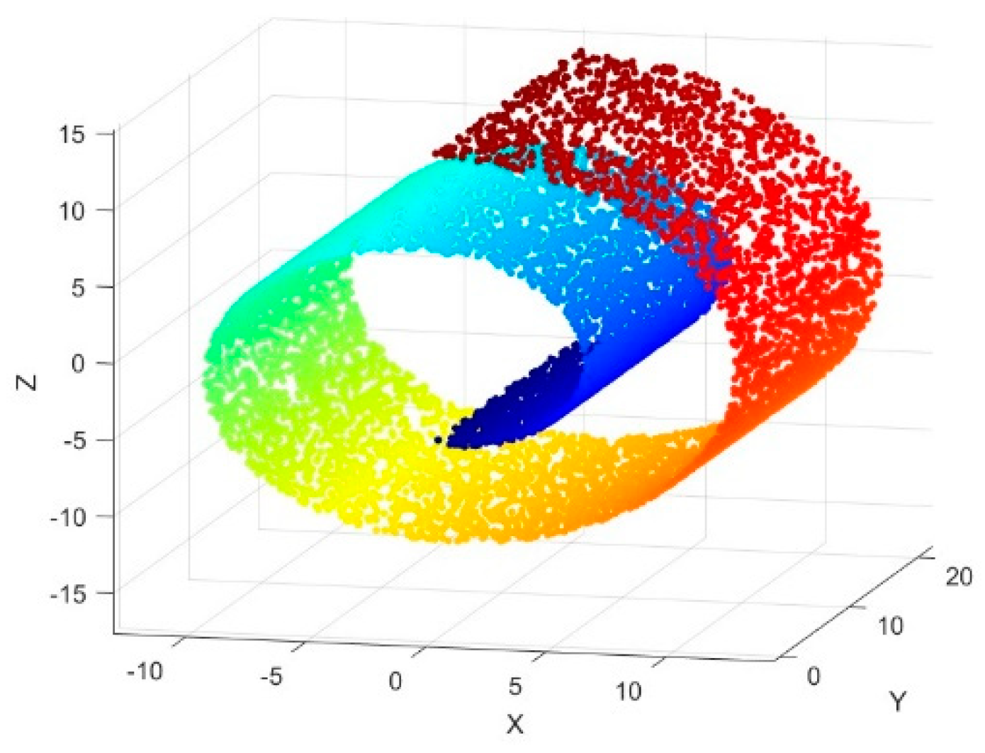
Figure 2.
The two-dimensional effect of reducing dimensionality with different k values in the Swiss roll data set: (a) k=50; (b) k=100; (c) k=200; (d) k=300.
Figure 2.
The two-dimensional effect of reducing dimensionality with different k values in the Swiss roll data set: (a) k=50; (b) k=100; (c) k=200; (d) k=300.
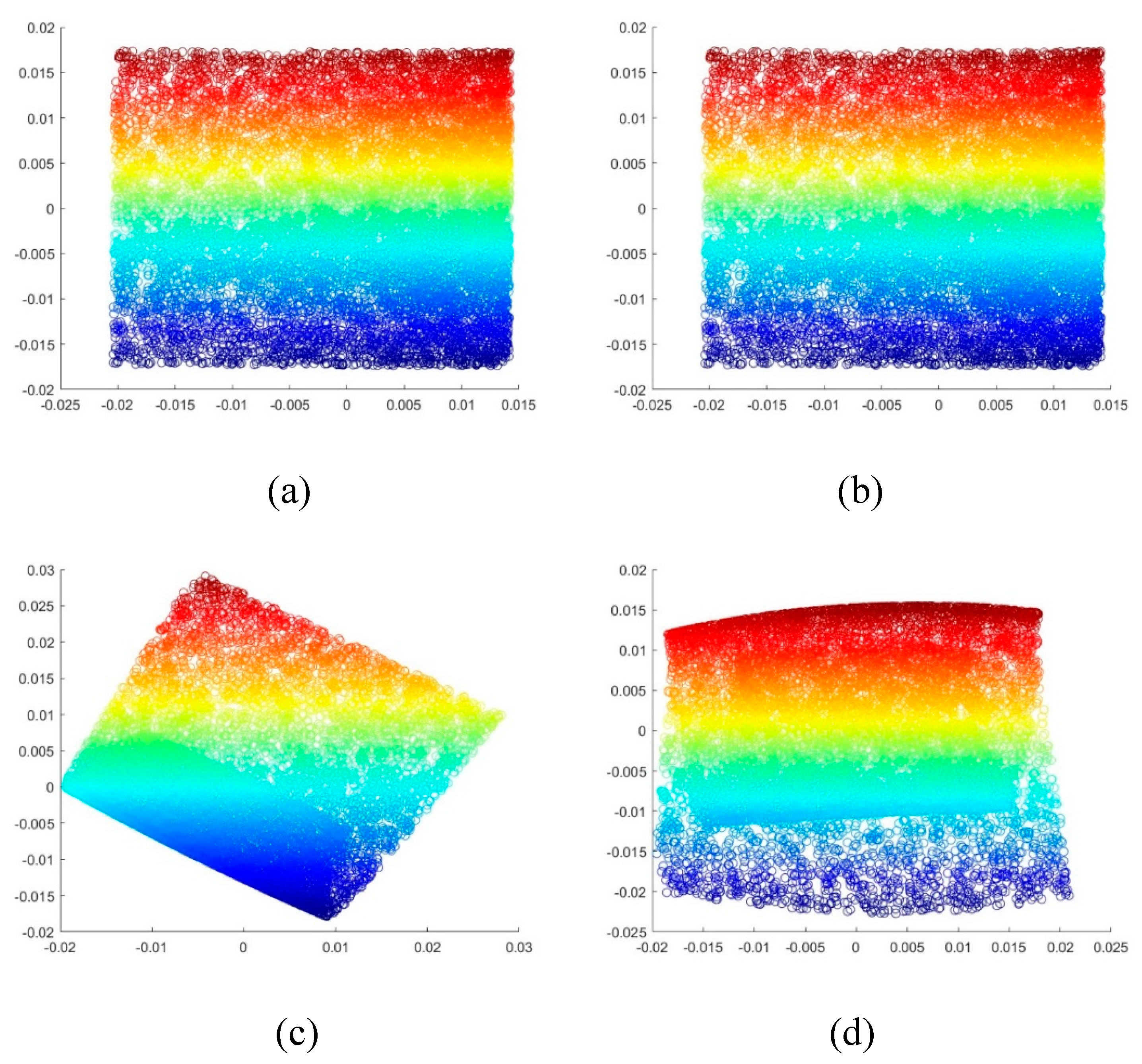
Figure 3.
Schematic diagram of hyperspectral image dimensionality reduction based on manifold learning technology.
Figure 3.
Schematic diagram of hyperspectral image dimensionality reduction based on manifold learning technology.
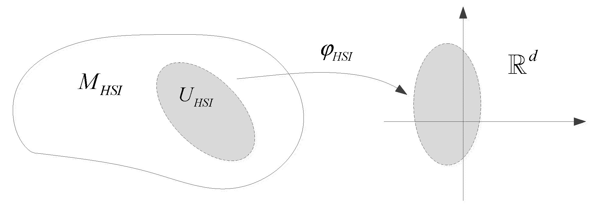
Figure 4.
Indian Pines data set:(a) False-color image;(b) Ground truth.
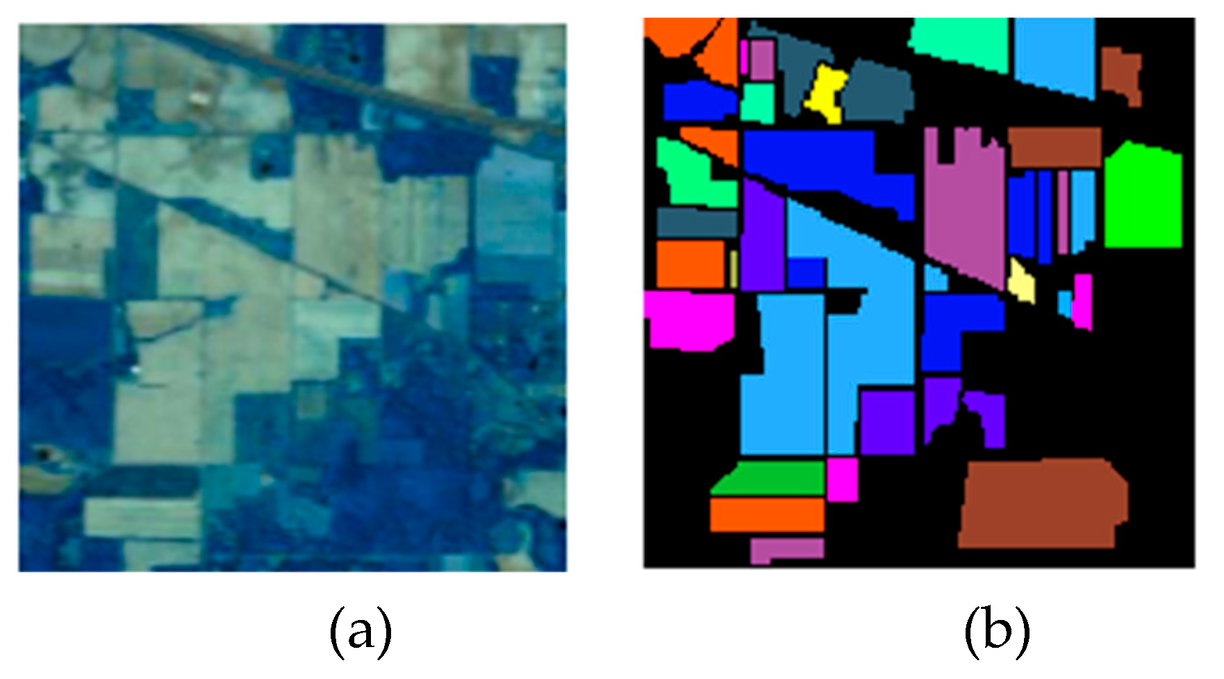
Figure 5.
Spectral characteristics curves of 16 features in the Indian Pines dataset.
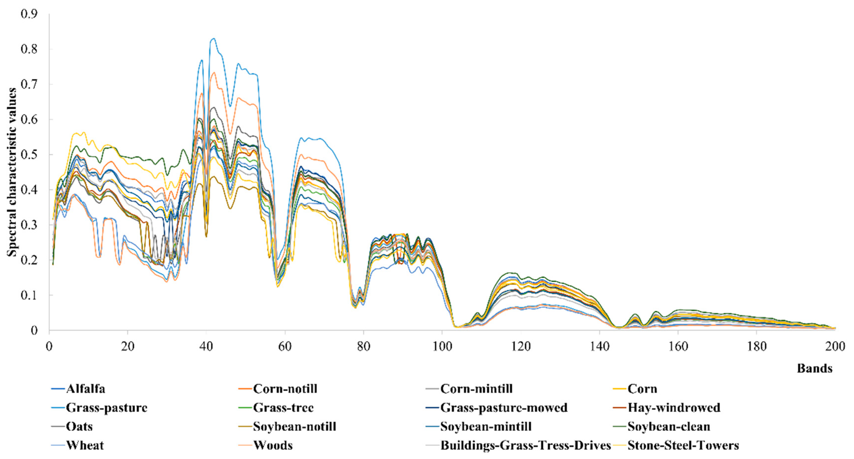
Figure 6.
Calculate the best neighborhood graph dimensionality reduction effect under different metrics when k=50 and d=2: (a) ED;(b) SAM;(c) SID.
Figure 6.
Calculate the best neighborhood graph dimensionality reduction effect under different metrics when k=50 and d=2: (a) ED;(b) SAM;(c) SID.
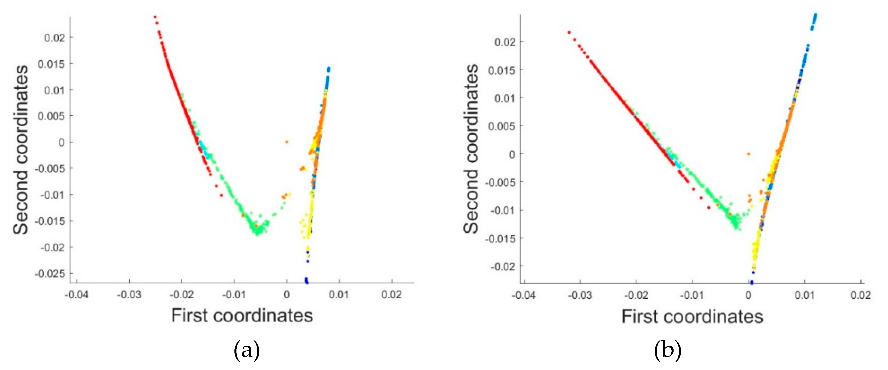
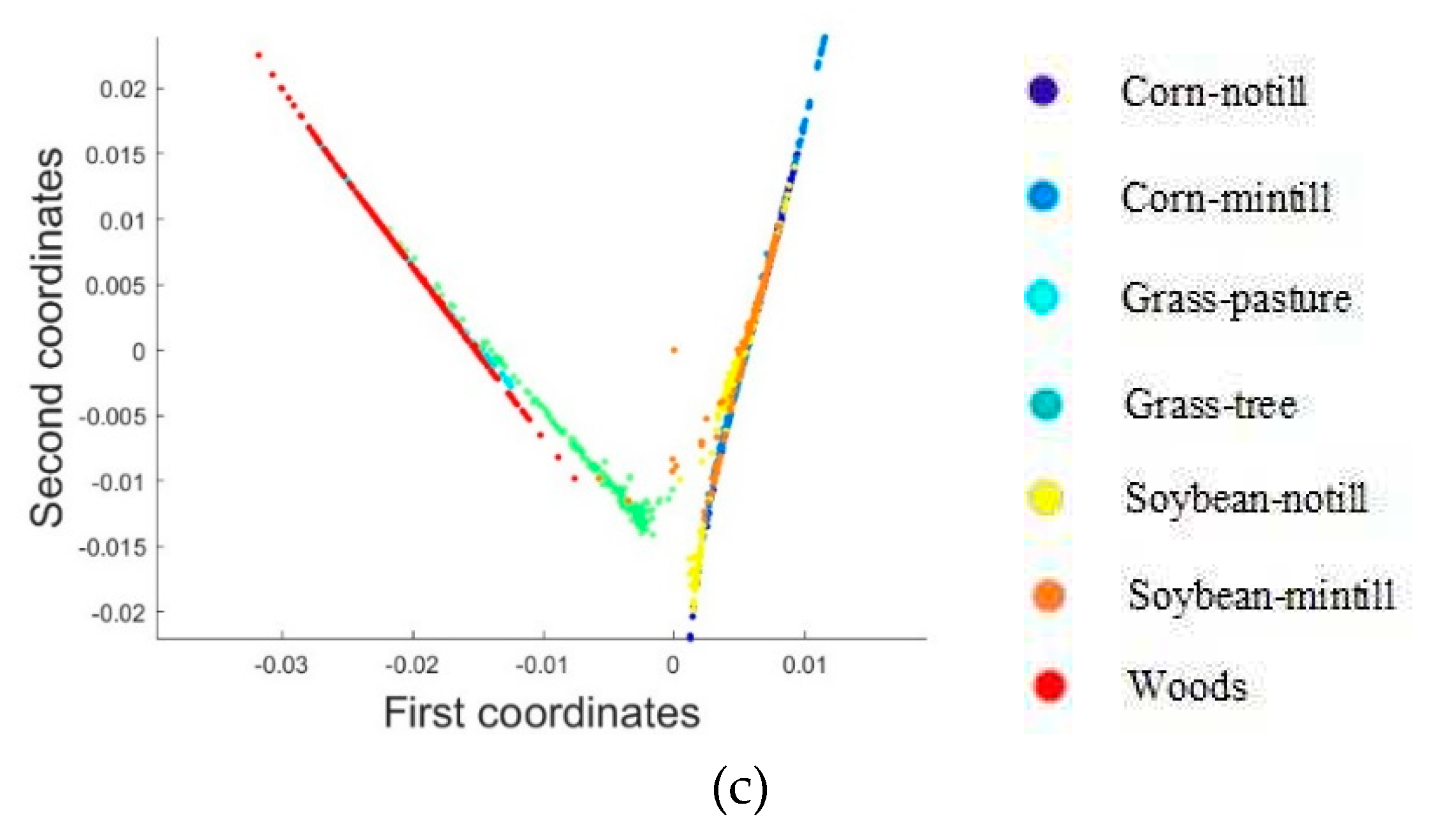
Figure 7.
Calculate the best neighborhood graph dimensionality reduction effect under different metrics when k=100 and d=2:(a)ED;(b) SAM;(c) SID.
Figure 7.
Calculate the best neighborhood graph dimensionality reduction effect under different metrics when k=100 and d=2:(a)ED;(b) SAM;(c) SID.
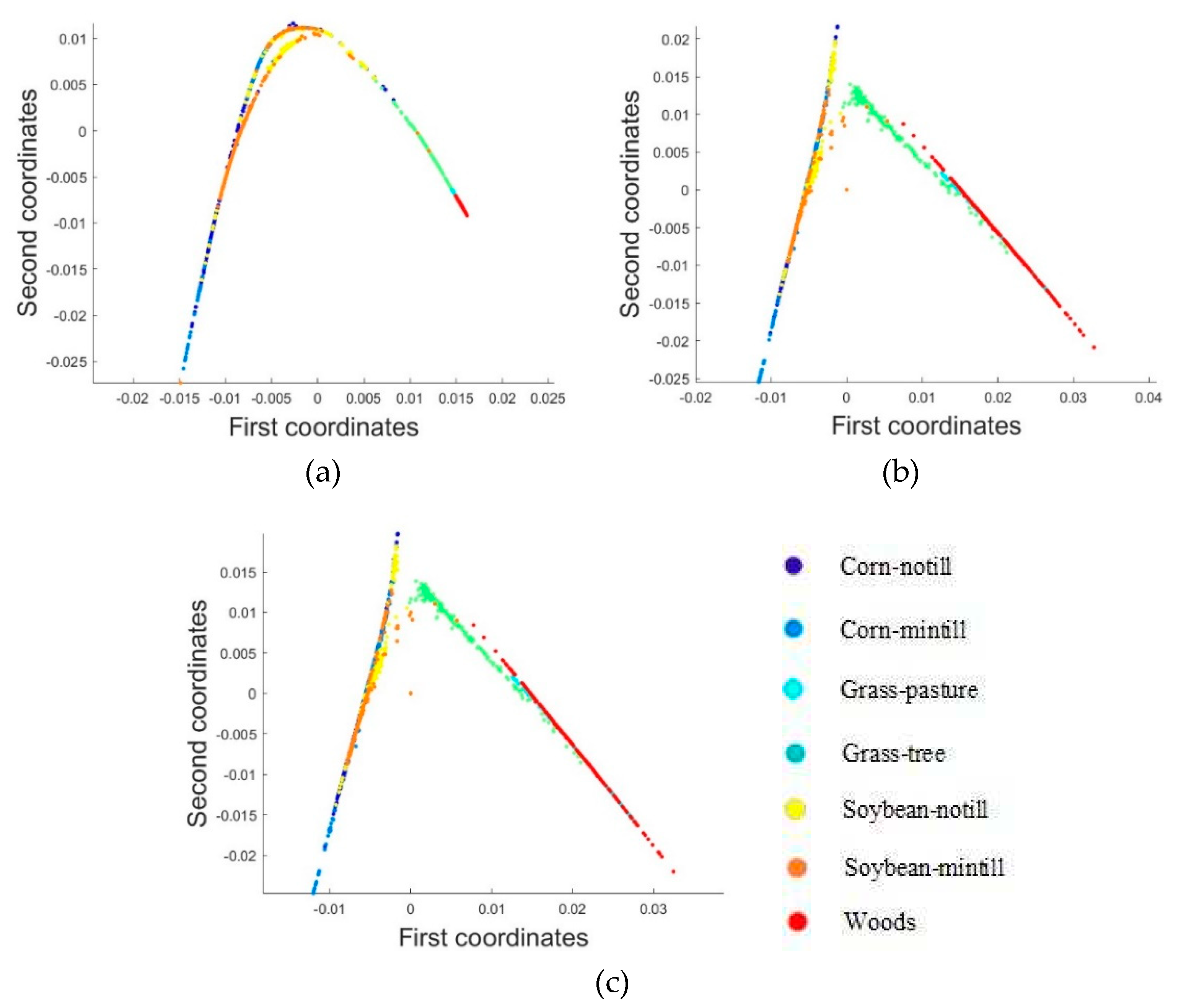
Figure 8.
Calculate the best neighborhood graph dimensionality reduction effect under different metrics when k=150 and d=2:(a) ED;(b) SAM;(c) SID.
Figure 8.
Calculate the best neighborhood graph dimensionality reduction effect under different metrics when k=150 and d=2:(a) ED;(b) SAM;(c) SID.
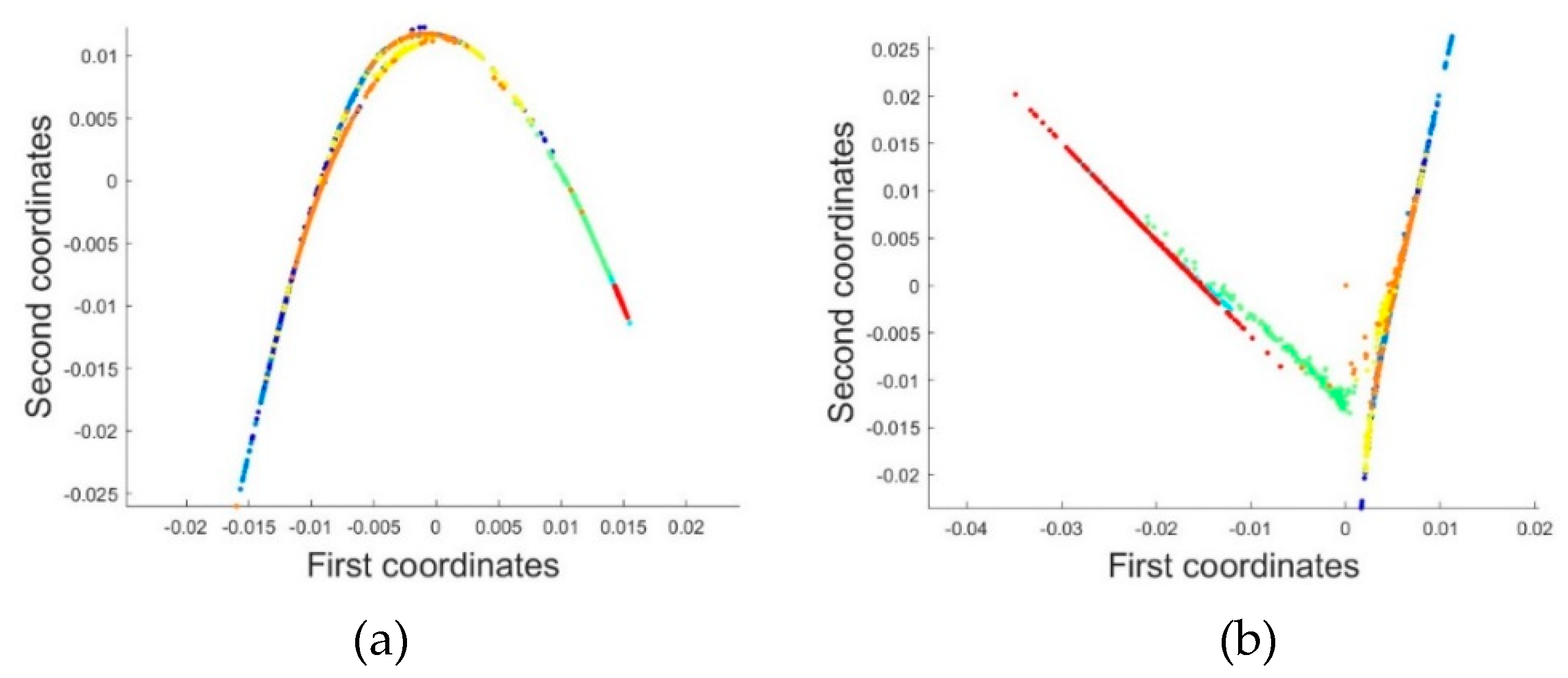
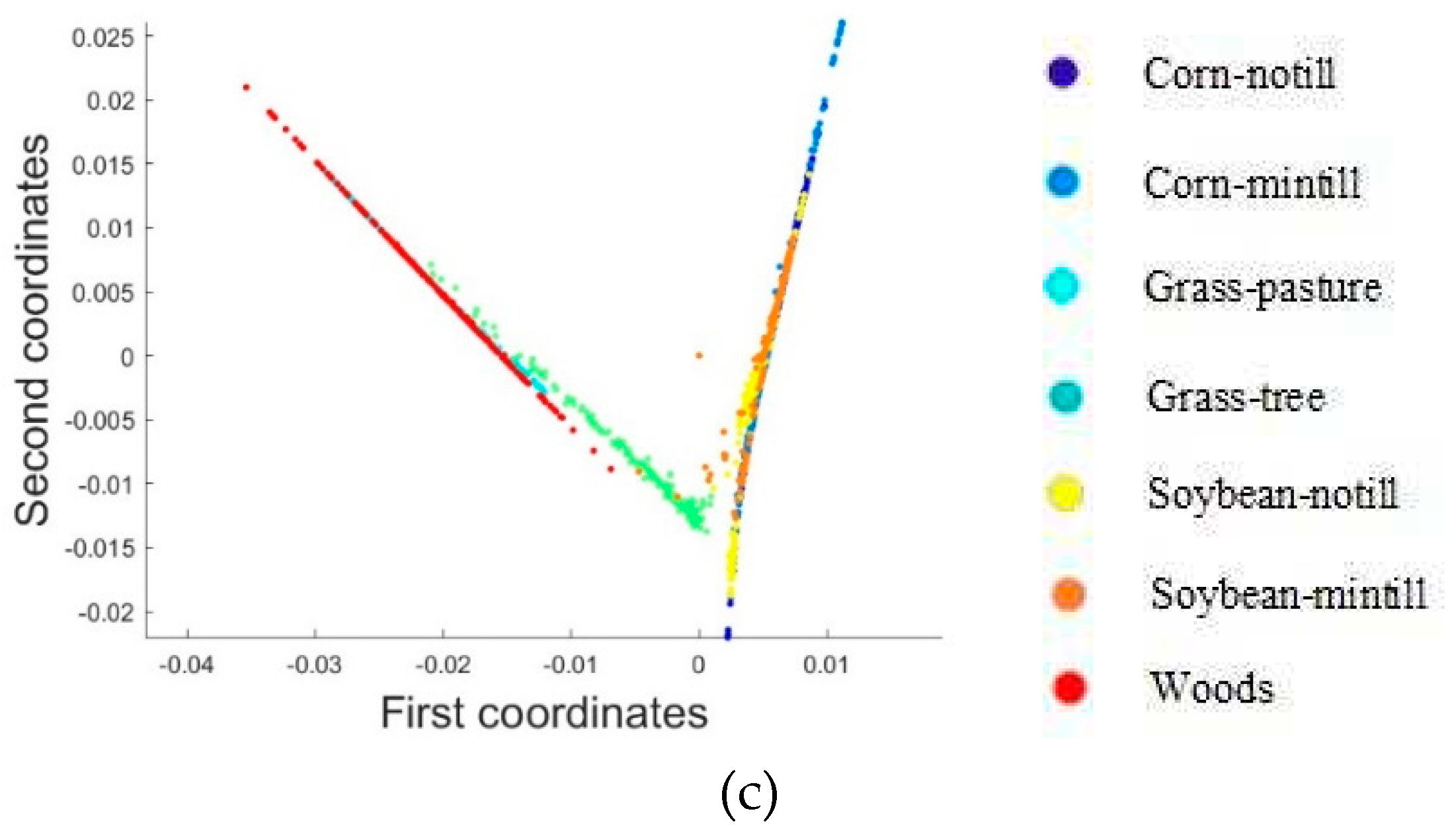
Figure 9.
Comparison of time and LTSA algorithm runtime for calculating the best neighborhood graph with three different metrics under different k/d values: (a) k=50 d=2; (b) k=100 d=2; (c) k=150 d=2.
Figure 9.
Comparison of time and LTSA algorithm runtime for calculating the best neighborhood graph with three different metrics under different k/d values: (a) k=50 d=2; (b) k=100 d=2; (c) k=150 d=2.
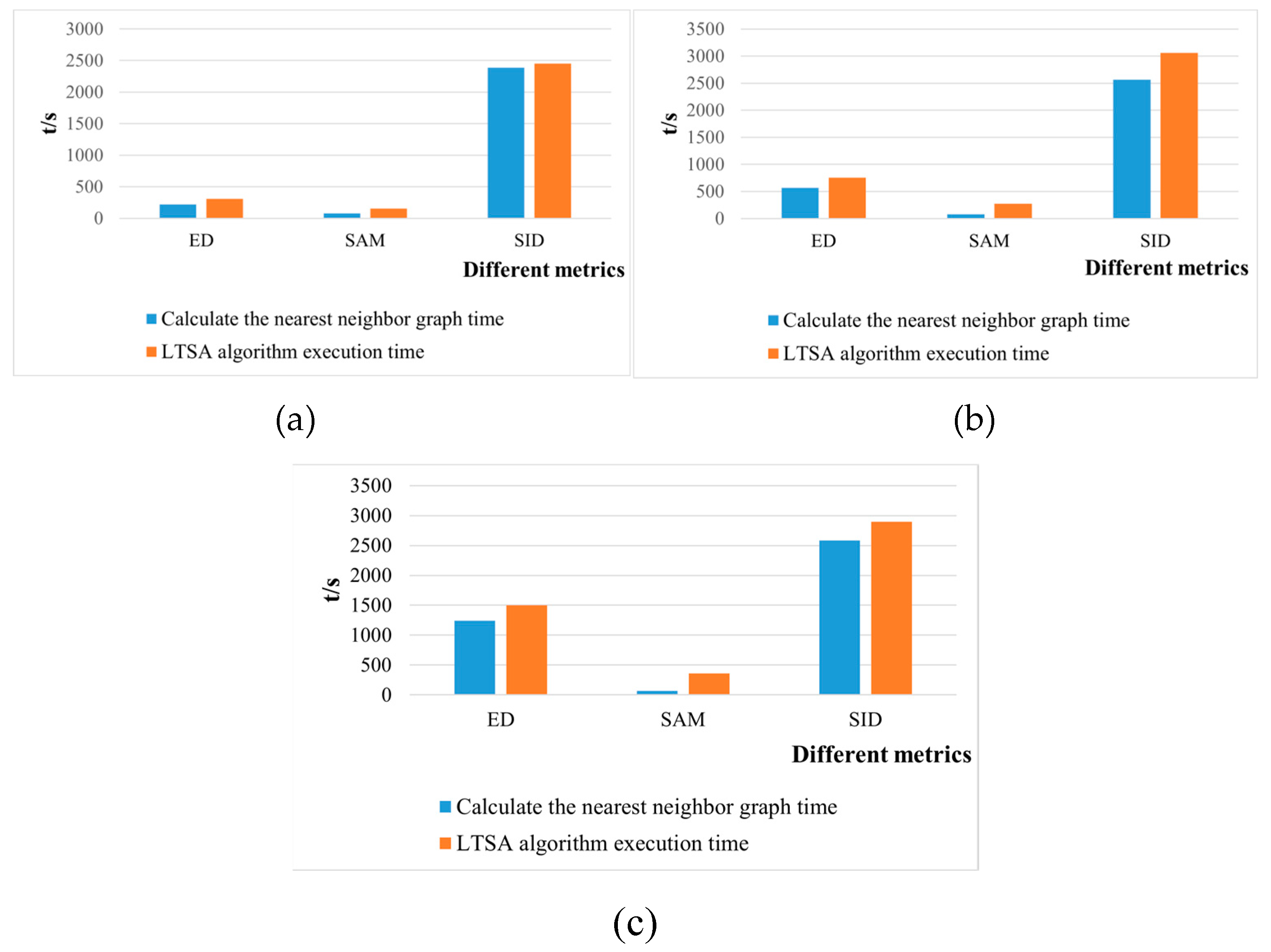
Figure 10.
Comparison between the computation time of nearest neighbor graph based on ED metric and the dimensionality reduction time of LTSA algorithm.
Figure 10.
Comparison between the computation time of nearest neighbor graph based on ED metric and the dimensionality reduction time of LTSA algorithm.
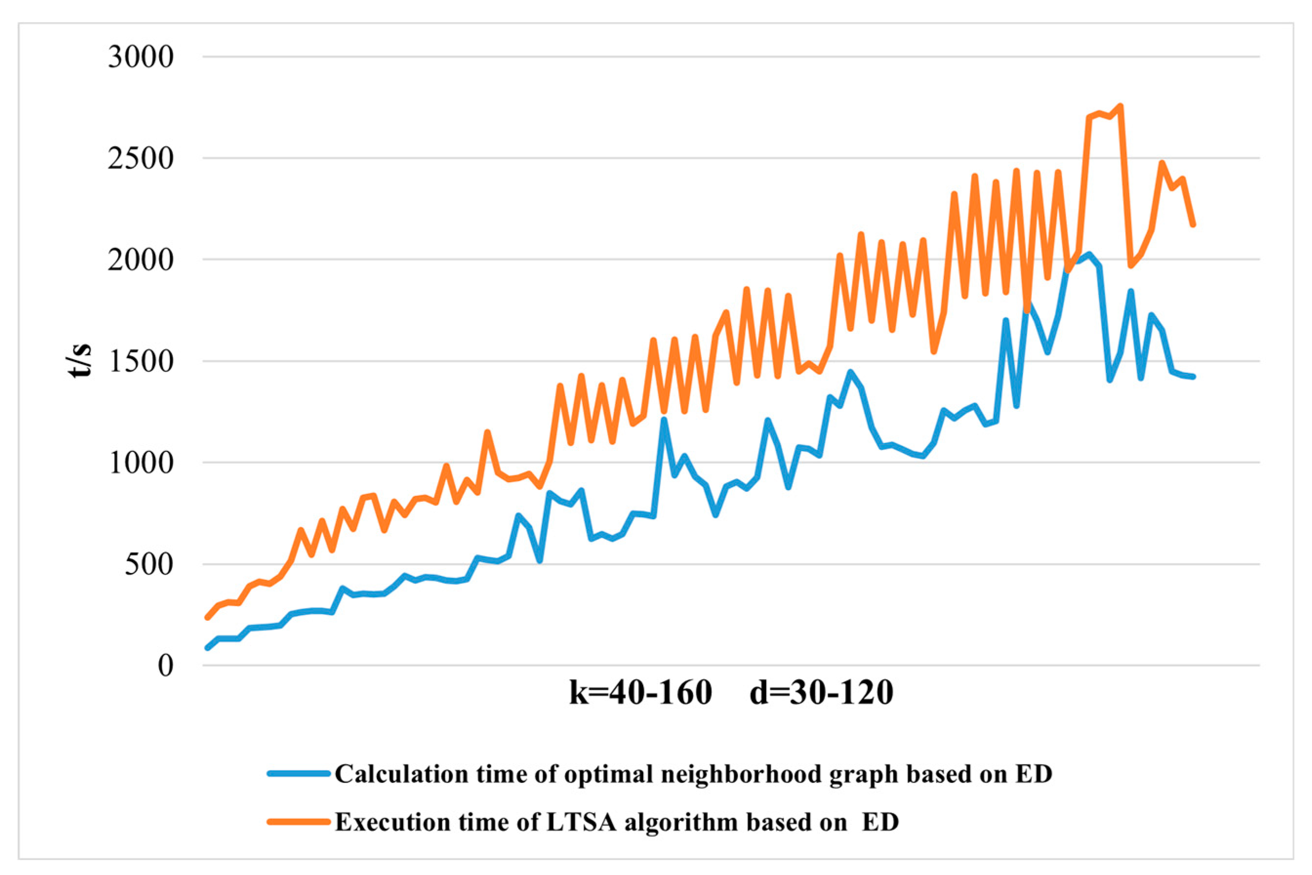
Figure 11.
Overall accuracy curve based on ED metric.
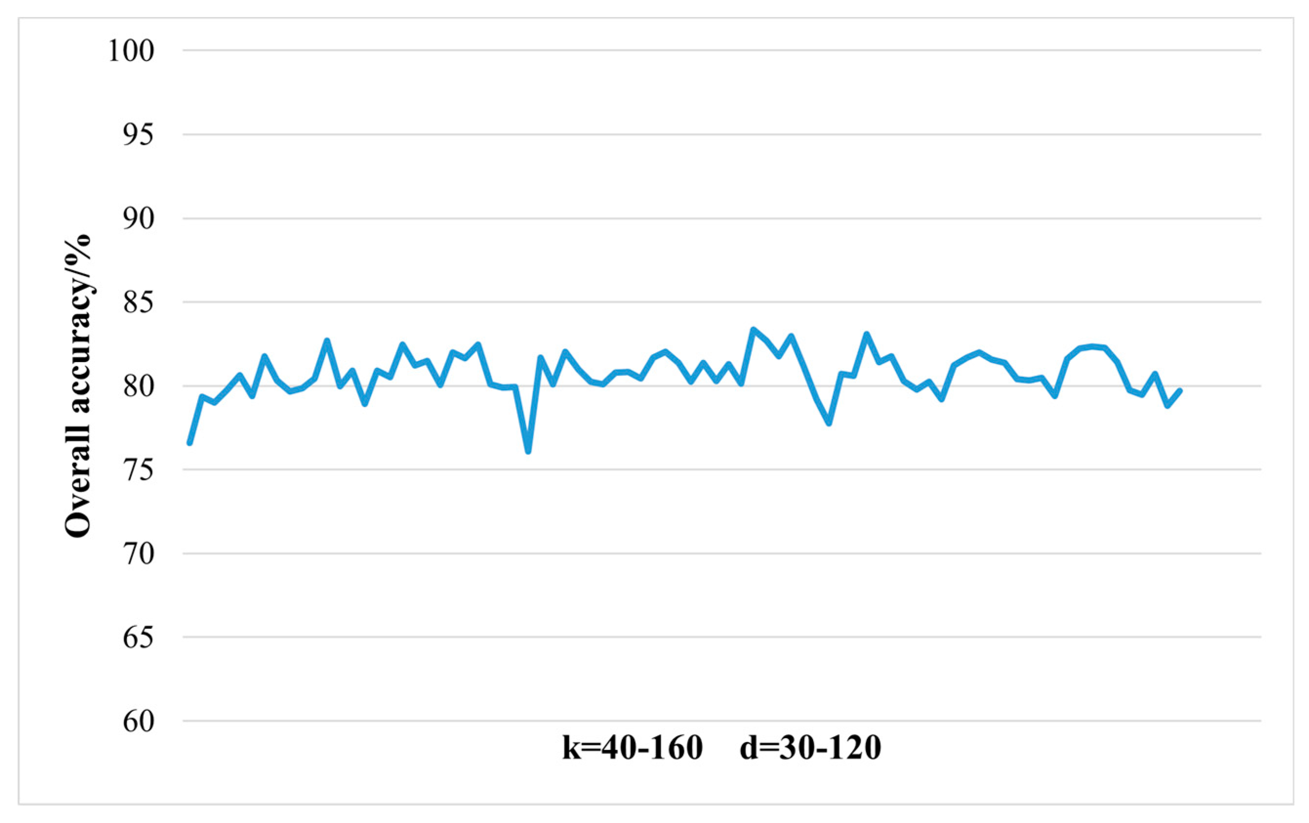
Figure 12.
Comparison of computation time of nearest neighbor graph based on SAM metric and dimensionality reduction time of LTSA algorithm.
Figure 12.
Comparison of computation time of nearest neighbor graph based on SAM metric and dimensionality reduction time of LTSA algorithm.
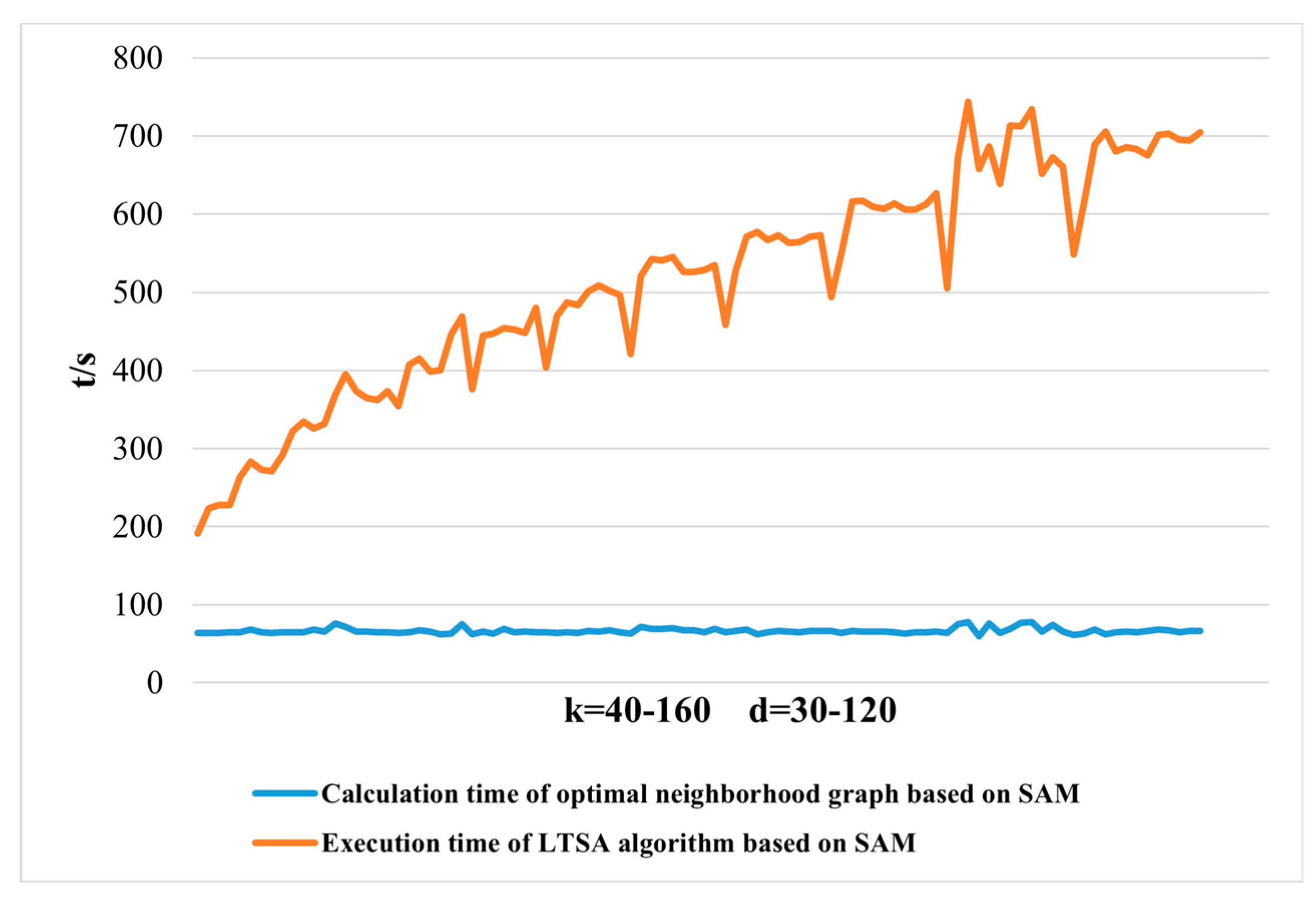
Figure 13.
Overall accuracy curve based on SAM metric.
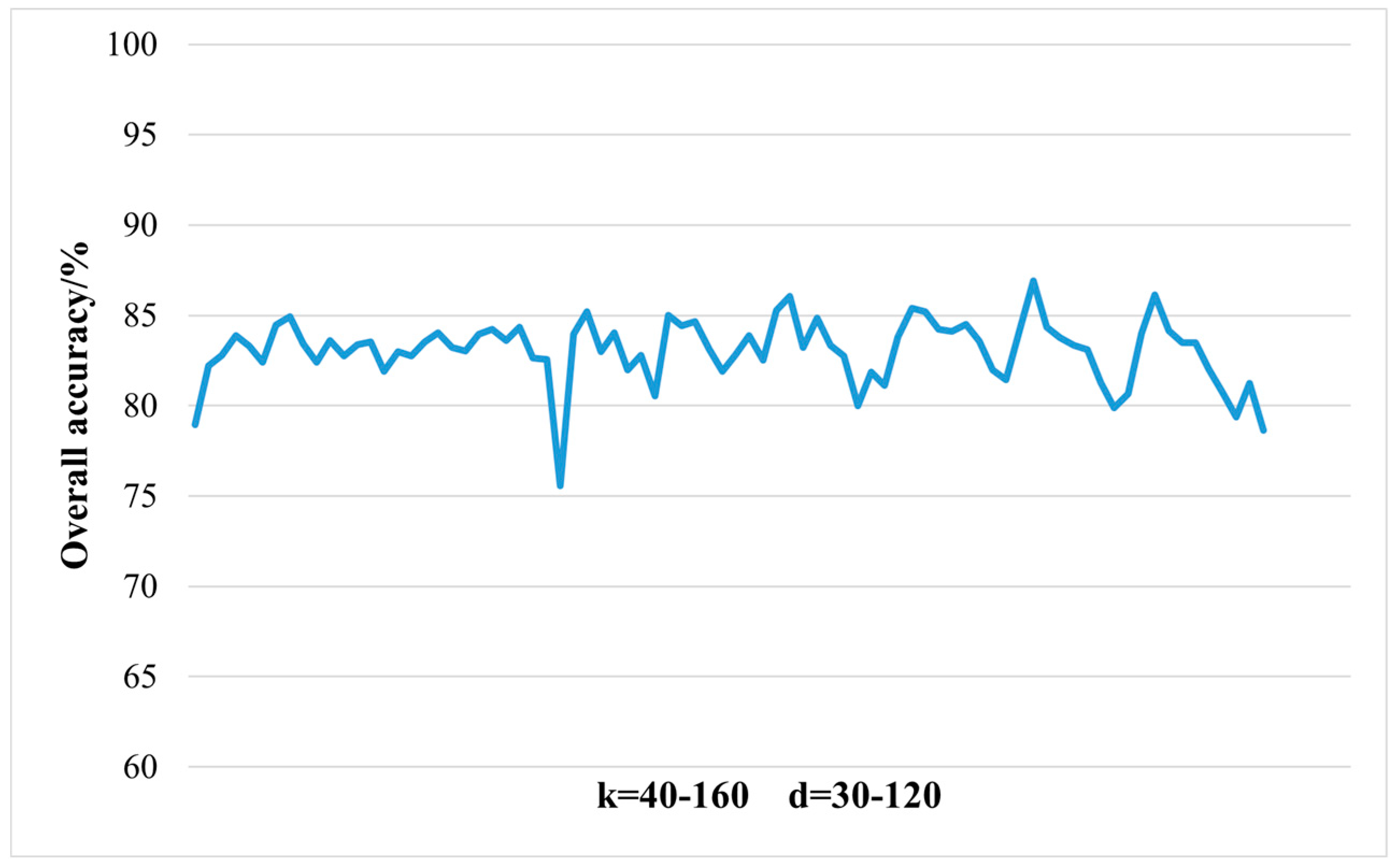
Figure 14.
Comparison of nearest neighbor graph calculation and LTSA algorithm running time based on SID metric.
Figure 14.
Comparison of nearest neighbor graph calculation and LTSA algorithm running time based on SID metric.
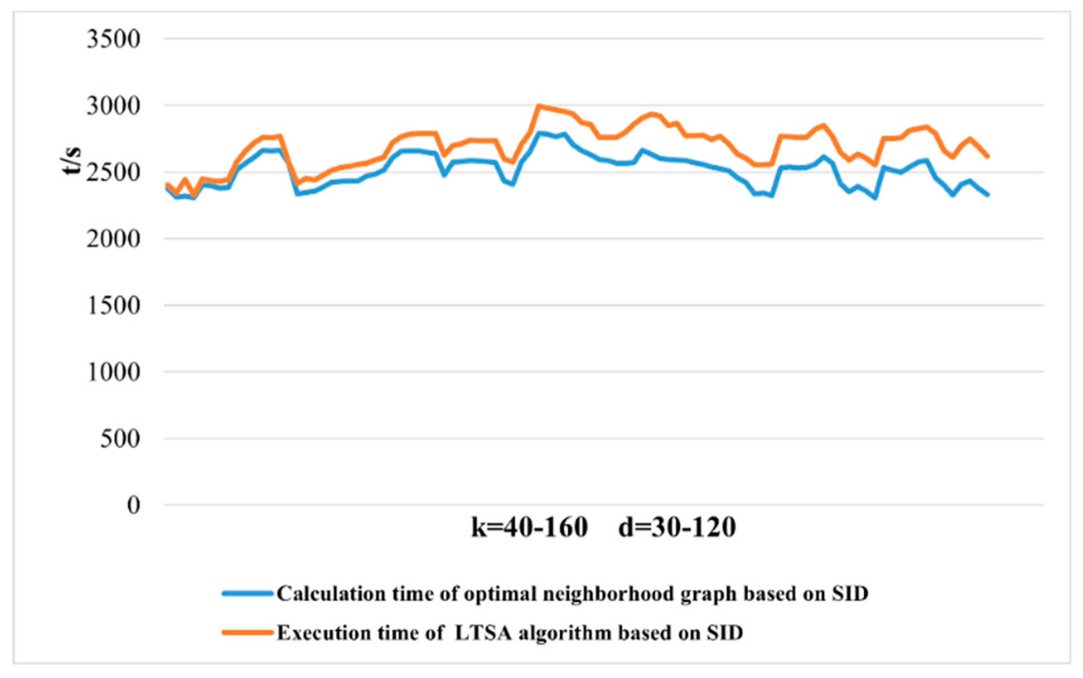
Figure 15.
Overall accuracy curve based on SID metric.
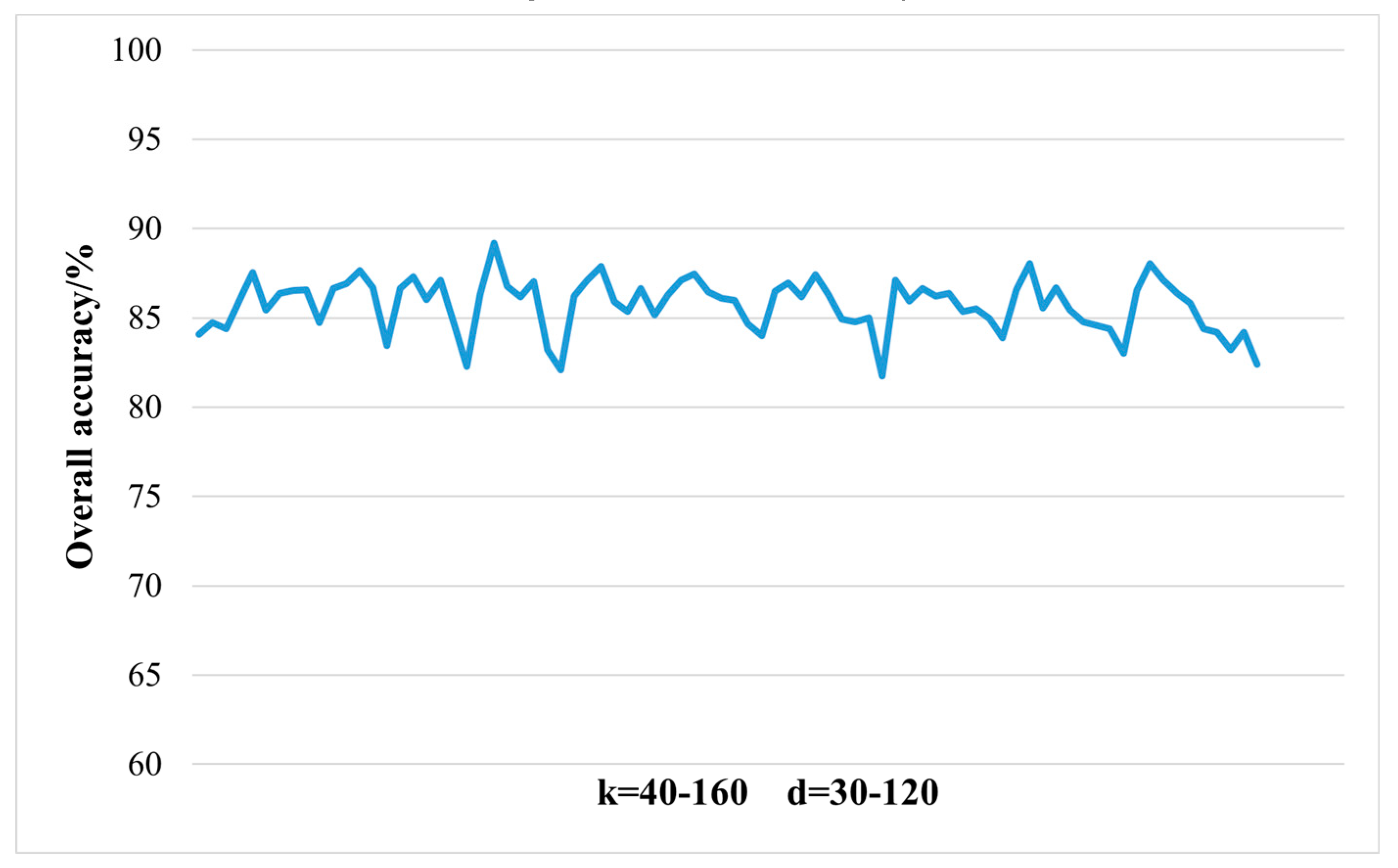
Figure 16.
Comparison of nearest neighbor graph calculation and LTSA algorithm running time with increasing k/d values under three different metrics.
Figure 16.
Comparison of nearest neighbor graph calculation and LTSA algorithm running time with increasing k/d values under three different metrics.
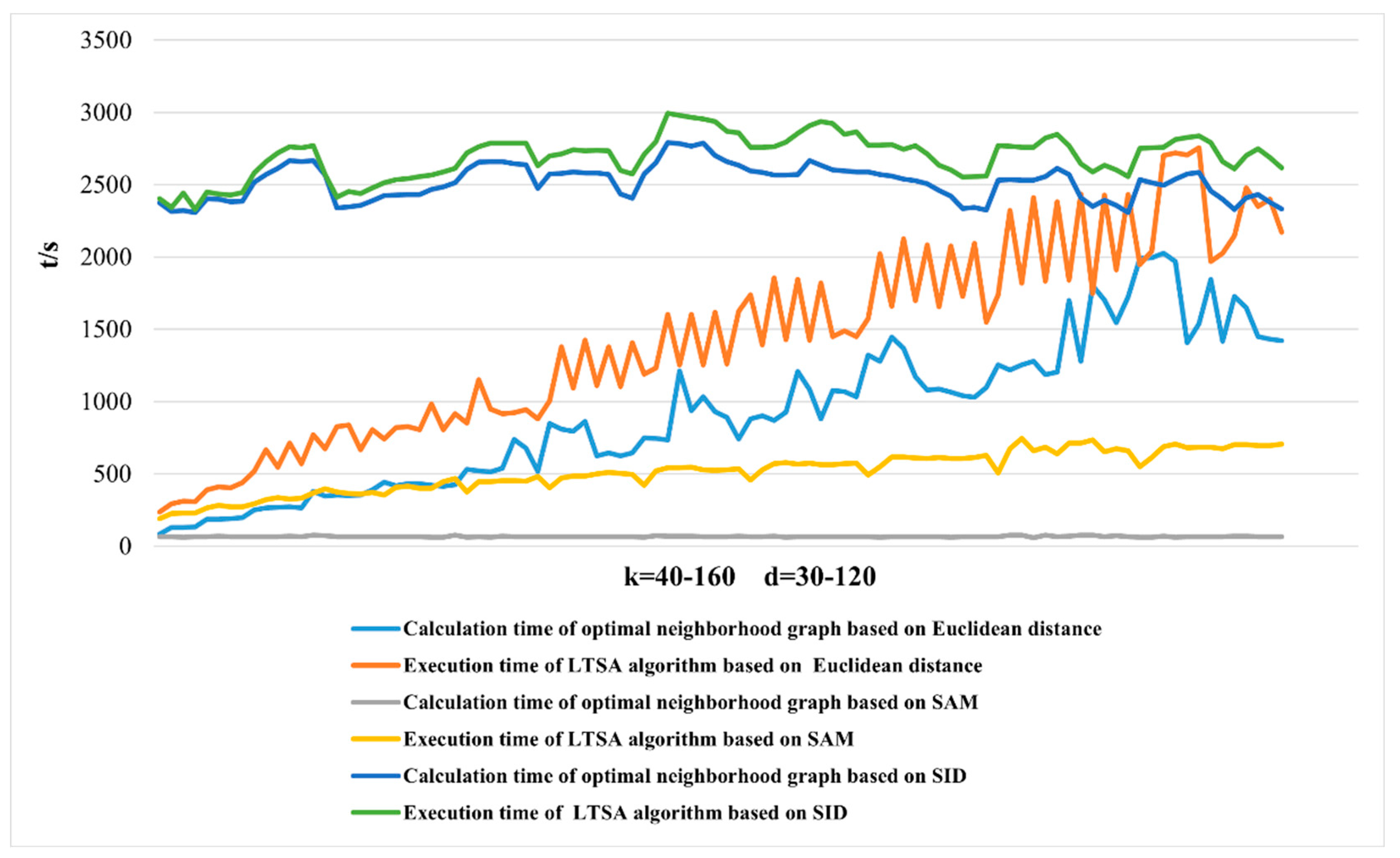
Figure 17.
Comparison of overall accuracy with increasing k/d values under three different metrics.
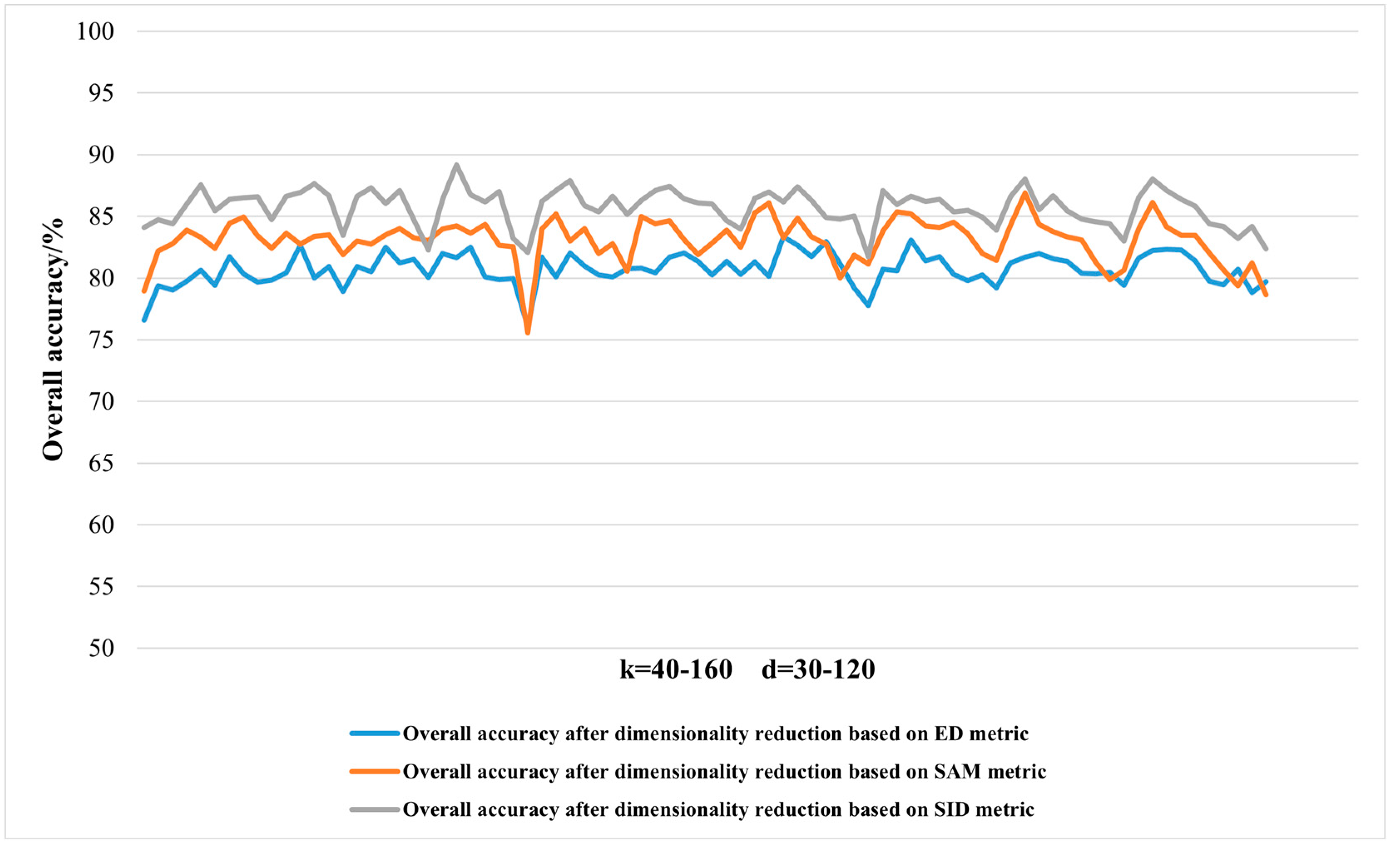

Table 1.
Comparison of geometric relationships and computational complexity of algorithms.
| Method | Geometric relationship | Global/Local Relationships | Computational complexity |
|---|---|---|---|
| Isomap | Point pair Geodesic Distance | Global | Very high |
| LLE | Local linear reconstruction relationship | Local | Low |
| LE | Local domain similarity | Local | Low |
| HLLE | Local isometry | Local | High |
| LTSA | Local coordinate representation | Global & Local | Low |
| MVU | Local distance | Global & Local | Very high |
Table 2.
Ground truth classes and sample numbers of Indian Pines.
| Category | Classification | Colour | Samples |
|---|---|---|---|
| 1 | Alfalfa | 46 | |
| 2 | Corn-notill | 1428 | |
| 3 | Corn-mintill | 830 | |
| 4 | Corn | 237 | |
| 5 | Grass-pasture | 483 | |
| 6 | Grass-tree | 730 | |
| 7 | Grass-pasture-mowed | 28 | |
| 8 | Hay-windrowed | 478 | |
| 9 | Oats | 20 | |
| 10 | Soybean-notill | 972 | |
| 11 | Soybean-mintill | 2455 | |
| 12 | Soybean-clean | 593 | |
| 13 | Wheat | 205 | |
| 14 | Woods | 1265 | |
| 15 | Buildings-Grass-Tress-Drives | 386 | |
| 16 | Stone-Steel-Towers | 93 |
Table 3.
Ground classification and division of Indian Pines data set.
| Category | Classification | Training samples | Testing samples |
|---|---|---|---|
| 1 | Alfalfa | 37 | 9 |
| 2 | Corn-notill | 1142 | 286 |
| 3 | Corn-mintill | 664 | 166 |
| 4 | Corn | 190 | 47 |
| 5 | Grass-pasture | 386 | 97 |
| 6 | Grass-tree | 584 | 146 |
| 7 | Grass-pasture-mowed | 22 | 6 |
| 8 | Hay-windrowed | 382 | 96 |
| 9 | Oats | 16 | 4 |
| 10 | Soybean-notill | 778 | 194 |
| 11 | Soybean-mintill | 1964 | 491 |
| 12 | Soybean-clean | 474 | 119 |
| 13 | Wheat | 164 | 41 |
| 14 | Woods | 1012 | 253 |
| 15 | Buildings-Grass-Tress-Drives | 309 | 77 |
| 16 | Stone-Steel-Towers | 74 | 19 |
| Total | 8199 | 2050 |
Table 4.
7 types of ground objects categories and sample sizes for visualization.
| Category | Classification | Samples |
|---|---|---|
| 2 | Corn-notill | 200 |
| 3 | Corn-mintill | 200 |
| 5 | Grass-pasture | 200 |
| 6 | Grass-tree | 200 |
| 10 | Soybean-notill | 200 |
| 11 | Soybean-mintill | 200 |
| 14 | Woods | 200 |
Table 5.
Based on ED metric, select different k/d values to calculate the optimal neighborhood graph and LTSA algorithm runtime, and calculate overall accuracy.
Table 5.
Based on ED metric, select different k/d values to calculate the optimal neighborhood graph and LTSA algorithm runtime, and calculate overall accuracy.
| k | d | The calculation time of the nearest neighbor graph/s | LTSA algorithm runtime/s | Overall accuracy/% |
|---|---|---|---|---|
| 40 | 30 | 85.0031 | 237.8442 | 76.5739 |
| 50 | 30 | 130.6625 | 293.6383 | 79.3558 |
| 40 | 130.5847 | 310.7664 | 79.0142 | |
| 60 | 30 | 185.5544 | 389.1228 | 79.7462 |
| 40 | 185.9724 | 411.4543 | 80.6274 | |
| 50 | 189.3846 | 401.9933 | 79.4046 | |
| … | … | |||
| 160 | 30 | 1988.9 | 1949.1 | 81.6008 |
| 40 | 1993.6 | 2038.6 | 82.2352 | |
| 50 | 2026.1 | 2701.1 | 82.3328 | |
| 60 | 1968 | 2721.4 | 82.284 | |
| 70 | 1406.8 | 2704.4 | 81.4056 | |
| 80 | 1538.6 | 2757.2 | 79.7462 | |
| 90 | 1844.3 | 1969.6 | 79.4543 | |
| 100 | 1415.9 | 2027 | 80.7223 | |
| 110 | 1726.4 | 2147 | 78.8189 | |
| 120 | 1650.1 | 2476.5 | 79.6974 |
Table 6.
Comparison of overall accuracy for different k/d values based on ED metric.
| Metric | k/d value | Overall accuracy/% | Kappa coefficient |
|---|---|---|---|
| ED | k=130 d=40 | 80.1367 | 78.9922 |
| k=130 d=50 | 83.3557 | 82.2112 | |
| k=130 d=60 | 82.6745 | 81.53 | |
| k=140 d=40 | 80.5759 | 79.4314 | |
| k=140 d=50 | 83.0649 | 81.9204 | |
| k=140 d=60 | 81.4056 | 80.2611 | |
| k=150 d=40 | 81.6984 | 80.5539 | |
| k=150 d=50 | 81.9912 | 80.8467 | |
| k=150 d=60 | 81.552 | 80.4075 |
Table 7.
Based on SAM distance metric, select different k/d values to calculate the optimal neighborhood graph and LTSA algorithm runtime, and calculate overall accuracy.
Table 7.
Based on SAM distance metric, select different k/d values to calculate the optimal neighborhood graph and LTSA algorithm runtime, and calculate overall accuracy.
| k | d | The calculation time of the nearest neighbor graph/s | LTSA algorithm runtime/s | Overall accuracy/% |
|---|---|---|---|---|
| 40 | 30 | 63.9568 | 191.6867 | 78.9395 |
| 50 | 30 | 63.9751 | 223.7559 | 82.2094 |
| 40 | 63.5359 | 227.2922 | 82.795 | |
| 60 | 30 | 64.3453 | 263.465 | 83.8687 |
| 40 | 67.7445 | 283.2065 | 83.2831 | |
| 50 | 64.7961 | 272.8833 | 82.4046 | |
| ·… | … | |||
| 160 | 30 | 61.4655 | 548.3659 | 83.9775 |
| 40 | 62.8563 | 614.0328 | 86.1137 | |
| 50 | 67.9539 | 688.9331 | 84.1615 | |
| 60 | 62.2563 | 705.472 | 83.4783 | |
| 70 | 64.5107 | 680.2691 | 83.4783 | |
| 80 | 63.3355 | 685.8673 | 82.0142 | |
| 90 | 64.663 | 683.0453 | 80.6964 | |
| 100 | 66.6848 | 675.4022 | 79.3787 | |
| 110 | 67.8423 | 701.4498 | 81.2333 | |
| 120 | 67.5131 | 703.186 | 78.6467 |
Table 8.
Comparison of overall accuracy based on SAM metric for different k/d values calculation.
| Metric | k/d values | Overall accuracy/% | Kappa coefficient |
|---|---|---|---|
| SAM | k=130 d=40 | 86.0649 | 84.9295 |
| k=130 d=50 | 83.2343 | 82.0989 | |
| k=130 d=60 | 84.8448 | 83.7094 | |
| k=140 d=40 | 85.3816 | 84.2462 | |
| k=140 d=50 | 85.1864 | 84.051 | |
| k=140 d=60 | 84.2103 | 83.0749 | |
| k=150 d=40 | 86.8946 | 85.7592 | |
| k=150 d=50 | 84.3568 | 83.2214 | |
| k=150 d=60 | 83.7711 | 82.6357 |
Table 9.
Based on SID distance metric, select different k/d values to calculate the optimal neighborhood graph and LTSA algorithm runtime, and calculate overall accuracy.
Table 9.
Based on SID distance metric, select different k/d values to calculate the optimal neighborhood graph and LTSA algorithm runtime, and calculate overall accuracy.
| k | d | The calculation time of the nearest neighbor graph/s | LTSA algorithm runtime/s | Overall accuracy/% |
|---|---|---|---|---|
| 40 | 30 | 2374.8 | 2403.4 | 84.0821 |
| 50 | 30 | 2313.3 | 2343.9 | 84.7165 |
| 40 | 2321.6 | 2443.8 | 84.3749 | |
| 60 | 30 | 2404 | 2450.9 | 85.9855 |
| 40 | 2398.3 | 2436.9 | 87.5472 | |
| 50 | 2382 | 2427.7 | 85.4486 | |
| ·… | … | |||
| 160 | 30 | 2533.4 | 2751 | 86.5223 |
| 40 | 2512.3 | 2754.6 | 88.0352 | |
| 50 | 2497.4 | 2757.6 | 87.108 | |
| 60 | 2536.8 | 2812.5 | 86.3759 | |
| 70 | 2574.5 | 2826.7 | 85.839 | |
| 80 | 2585 | 2837.9 | 84.3749 | |
| 90 | 2456.9 | 2789.4 | 84.1797 | |
| 100 | 2398.6 | 2658.9 | 83.2036 | |
| 110 | 2329.7 | 2609.3 | 84.1797 | |
| 120 | 2409.5 | 2700.6 | 82.3739 |
Table 10.
Comparison of overall accuracy for different k/d values based on SID metric.
| Metric | k/d values | Overall accuracy/% | Kappa coefficient |
|---|---|---|---|
| SID | k=130 d=40 | 86.9615 | 85.8012 |
| k=130 d=50 | 86.1807 | 85.0204 | |
| k=130 d=60 | 87.4008 | 86.2405 | |
| k=140 d=40 | 85.9367 | 84.7764 | |
| k=140 d=50 | 86.6199 | 85.4596 | |
| k=140 d=60 | 86.2295 | 85.0692 | |
| k=150 d=40 | 88.0352 | 86.8749 | |
| k=150 d=50 | 85.5462 | 85.5462 | |
| k=150 d=60 | 86.6687 | 85.5084 |
Table 11.
Overall accuracy and Kappa coefficient under different metrics.
| Metric | k/d values | Overall accuracy/% | Kappa coefficient |
|---|---|---|---|
| ED | k=130 d=50 | 83.3557 | 82.2112 |
| SAM | k=150 d=40 | 86.8946 | 85.7592 |
| SID | k=150 d=40 | 88.0352 | 86.8749 |
Disclaimer/Publisher’s Note: The statements, opinions and data contained in all publications are solely those of the individual author(s) and contributor(s) and not of MDPI and/or the editor(s). MDPI and/or the editor(s) disclaim responsibility for any injury to people or property resulting from any ideas, methods, instructions or products referred to in the content. |
© 2024 by the authors. Licensee MDPI, Basel, Switzerland. This article is an open access article distributed under the terms and conditions of the Creative Commons Attribution (CC BY) license (http://creativecommons.org/licenses/by/4.0/).
Copyright: This open access article is published under a Creative Commons CC BY 4.0 license, which permit the free download, distribution, and reuse, provided that the author and preprint are cited in any reuse.


