Submitted:
11 January 2024
Posted:
14 January 2024
You are already at the latest version
Abstract
This study proposes a methodology for identifying time intervals in which time-of-use (ToU) energy tariffs can be set. This is achieved by analyzing the variability in electric power demand and esti-mating the potential for demand flexibility. The proposed methodology is as follows: first, data preprocessing is performed, focusing on the organization and cleaning of individual consumption records. Subsequently, the data are processed and classified by using consumption variability analysis and clustering techniques. Then, representative clusters are selected and time intervals are analyzed to identify periods of high electric power consumption variability. This methodology was tested with real data from smart meters in the Colombian electrical system, in which time intervals with potential for settinh ToU tariffs were ultimately identified.
This work promotes the implementation of demand response strategies that enhance sustainability and facilitate the transition to a more resilient energy landscape both nationally and internationally. The findings are expected to contribute to the formulation of tariff schemes that encourage con-scious changes in electric energy consumption patterns.
Keywords:
Demand flexibility
; demand variability
; electric power
; demand response (DR)
; data analysis
; differential tariff scheme
; Time-of-use (ToU)
; Advanced Metering Infrastructure (AMI)
; smart metering
; smart meters
1. Introduction
Growing concern for the care and conservation of the planet has led to major global changes in the approach to environmental issues. From the United Nations Framework Convention on Climate Change in 1992 to the historic Paris Agreement in 2015, international commitments have been made to reduce greenhouse gas emissions and combat climate change [1,2].
In response to these commitments, regional organizations and governments have implemented policies and guidelines to achieve specific goals in environmental protection and reduction of emissions. Examples include the European Green Deal, which aims to reduce greenhouse gas emissions by 55% by 2030, and Colombia’s CONPES 4075, which aims to reduce CO2 emissions by 51% by 2030 and achieve carbon neutrality by 2050 [3,4].
In this context, the transition to renewable energy sources, such as solar and wind, has accelerated. However, power generation from these sources is challenging due to their high variability and dependence on environmental conditions. This poses challenges in accurately predicting energy generation and in the stability of supply [5,6].
In light of this situation, smart grids have emerged as a promising solution to integrate renewable energy generation into the traditional electrical grid [7]. These grids require real-time information provided by smart meters, which measure electrical energy consumption and other parameters. The installation of smart meters has significantly grown worldwide, driven by government policies and regulations. By 2024, Asia-Pacific, Europe, and the United States are expected to lead the market with millions of meters installed in each region [7].
The use of smart meters has generated a large amount of data, as they can collect information at in intervals of seconds, minutes, or hours [8]. This data availability has spurred research focused on improving energy efficiency and reducing consumption in both residential and industrial contexts. One such are of research is Demand Response (DR), which seeks to change the end-users’ consumption patterns to smooth consumption peaks [9,10]. Demand Response integrates price incentive programs to change end-users’ consumption patterns, achieving stability and balance of energy resources in addition to providing economic efficiency to network stakeholders. Methods such as Real-Time Pricing (RTP), Time-of-Use (ToU) Pricing, and Critical Peak Pricing (CPP) have been proposed, with ToU and RTP being the most widely used. TOU pricing is a rate in which the energy price varies in time intervals ranging from hours to days or weeks. The latter is preferred by both network operators and consumers [11].
This article presents a method for identifying time intervals for differential electricity pricing, with a particular focus on the Time-of-Use pricing (ToU) approach, by using data analysis techniques based on information collected by smart meters. This method focuses on identifying those time intervals in which the flexibility of electric energy demand is most notable and, therefore, strategic for tariff implementation. The development of the method is based on the premise that a user who shows high variability in his consumption over a given time interval is more likely to show flexibility in his energy consumption during the same period.
2. Conceptual Framework
This section explores two concepts fundamental to this research: demand response and electric demand flexibility. On the one hand, demand response highlights the active role of consumers in adapting their electrical consumption in response to external stimuli, thereby contributing to more efficient energy management. On the other hand, demand flexibility refers to the ability of users to modify their consumption patterns over time, whether by increasing, decreasing, or shifting their electrical energy consumption. Both concepts are helpful in understanding and improving the efficiency and resilience of modern energy systems.
Demand Response (DR)
Demand response involves adjustments in the electrical consumption of users in response to changes in electricity prices, economic incentives, or guidelines from grid operators. This practice transforms consumers from passive entities to active agents in energy management, which allows them to save energy and contribute to grid stability through load flexibility. Currently, DR is evolving into a more comprehensive modality: Integrated Demand Response (IDR), which comprises different energy sources such as electricity, thermal, and natural gas. This evolution allows users not only to modify their electricity consumption, but also to choose between different energy sources. DR is part of an approach towards smart energy management that aims to maximize the aggregate benefits of smart energy systems and the daily profits of electricity companies [12].
Electric Demand Flexibility
Flexibility in electrical systems has become increasingly important due to the transition to renewable generation sources like solar and wind. These energies, despite their importance in the energy transition, pose challenges due to their variable and uncertain nature. Flexibility, in this context, refers to the ability of the electrical system to adapt reliably and cost-effectively to variations in electrical generation and demand over all time scales. Traditionally focused on generation, flexibility now also encompasses areas such as demand response, energy storage, and dispatchable distributed generation. It is fundamental to the effective integration of renewable energy, impacts system reliability and costs, and contributes to system resilience [13].
In the context of buildings, demand flexibility is the ability to adapt energy demand and generation to user needs, the electrical grid, and climatic conditions. It is achieved by modifying load profiles, such as demand reduction or shifting, and can be of two types: implicit, related to the adaptation of consumer behavior to price signals, and explicit, which requires the intervention of an aggregator and is marketable in energy markets. These strategies make it possible to manage consumption more efficiently, adapt to the requirements of the grid, and reduce the operating costs of buildings [14].
In the context of demand response, the flexibility of users is used to induce adjustments in the load profile of the electrical grid. This flexibility is implicit and depends on the behavior and preferences of consumers regarding their energy use. Understanding user flexibility requires a detailed analysis of their consumption patterns and their willingness to modify them. This study proposes a method for estimating user flexibility by examining the variability in their electrical energy consumption. The premise underlying our research is that greater variability in consumption may indicate a higher degree of user load flexibility.
3. Related Works
Demand Response (DR) is an approach aimed at modifying the electricity consumption patterns of various types of users, such as residential and industrial. This change is made in response to energy price signals or incentives to reduce consumption in order to balance electricity prices in the market and respond to operational or reliability needs of the system, such as the balance between consumed and generated energy [15]. DR facilitates the integration of renewable energy sources into the electrical system, maintaining harmony between the unpredictable generation of these sources and consumption.
As discussed above, demand flexibility is the ability of users to modify their electricity consumption over a given time, whether by increasing, decreasing, or shifting their consumption. This ability is key to the effective implementation of DR strategies, so it is essential to assess the demand flexibility potential of a group of users.
The flexibility of a user can be determined by knowing his internal load, that is, by identifying the appliances and devices used and his flexibility of use at different times. Load Monitoring (LM), which employs data analysis techniques, statistical tools, and others, is used to identify these devices. Another way to assess flexibility is by reviewing the DR strategies implemented and the users’ response to them. Some of the research conducted in Load Monitoring (LM) and Demand Response (DR) is presented below.
Load Monitoring (LM)
LM can be divided into three main categories: Intrusive Load Monitoring (ILM), Non-Intrusive Load Monitoring (NILM), and other methods. The ILM methodology, which assigns a meter to each appliance, can be costly and has connectivity issues. Therefore, the NILM methodology has been explored; this estimates the individual consumption of appliances by disaggregating the overall consumption by using algorithms. NILM is subdivided into Machine Learning (ML) techniques, Pattern Matching (PM), and single channel Source Separation (SS) [16].
The research by Tao et al. [17] presents a Load Monitoring (LM) methodology using the Non-Intrusive Load Monitoring (NILM) technique to optimize the energy purchase and sale operations in a microgrid. The methodology focuses on the disaggregation of high energy demand appliances, such as air conditioners, heaters, and ventilation systems, employing a multitask sequence-to-now learning structure with convolutional neural networks. Additionally, the authors propose a hidden Markov model-based method to support the microgrid’s bidding decisions in the energy market. Simulations reveal that this approach allows the microgrid operator to reduce consumption and load costs, as well as generate additional revenue by selling surplus energy in the market.
A study by Lilu et al. [18] presents a Pattern Matching (PM) methodology for electrical load disaggregation using the Affinity Propagation (AP) clustering algorithm. This method involves using training data to create appliance consumption templates in terms of reactive and real power, followed by temporal segmentation of the dataset and marking of the appliance states. A time-segmented state probability (TSSP) matrix is introduced for each appliance to improve speed and accuracy in load disaggregation. The effectiveness of the method was demonstrated through tests on the AMPds2 database (composed of two years of electricity consumption records from users in Canada), which showed a 96% success rate in load state identification and 86% accuracy in load decomposition.
In a related work, Ekanayake et al. [19] propose a NILM approach that integrates Appliance Usage Patterns (AUP) to optimize active load identification and prediction. This method starts with learning AUPs from a residence using NILM algorithms based on spectral decomposition, followed by adjusting the a priori probabilities of the devices through a fuzzy system. The effectiveness of the method was evaluated on standard databases, showing improvements in active load estimation. Additionally, this information was used to forecast the total active energy consumption in a set of homes, with promising results in predicting energy consumption five minutes ahead of the actual time.
Demand Response (DR)
Demand Response (DR) is used to mitigate peak electricity consumption or power peak-to-average ratio (PAR), mainly through real-time pricing (RTP) [20]. DR integrates price incentive programs to modify users’ consumption patterns, achieve stability and balance of energy resources, and provide economic benefits. However, tariff schemes like RTP and Time-of-Use pricing (ToU) can induce new consumption peaks during off-peak hours. ToU in particular is a dynamic rate that varies over intervals ranging from hours to days and is preferred by both network operators and consumers.
In this context, Fraija et al. [11] present a methodology that employs a Demand Response Aggregator (DRA) to create Time-of-Use (ToU) tariffs based on next-day discounts (DB-ToU). The purpose of this strategy is to leverage the flexible demand of residential users to smooth energy consumption curves. The DRA analyzes customer behavior regarding energy use based on their response to incentive policies, implementing daily pricing schemes and communicating price signals to manage demand and reduce peak load. This approach includes collecting consumption profiles, calculating rewards, and formulating future policies, using reinforcement learning to optimize DRA performance. This user-privacy-prioritization method has proven effective in improving the quality of the aggregated load profile without significantly impacting the aggregator’s revenues.
A similar proposal is made by Nawaz et al. [20], who develop a framework for efficient demand control in the Smart Grid by using data from the Advanced Metering Infrastructure (AMI) network. This framework is composed of four main components: (i) energy distribution companies, (ii) a module for predicting demand and pricing rates based on demand response, (iii) AMI metering infrastructure, and (iv) demand-side energy management. For energy management, the use of the Binary Particle Swarm Optimization (BPSO) algorithm is proposed to regulate internal consumption in response to network operator incentives. In addition, the prediction module uses a multilayer perceptron trained with historical consumption data. This dataset includes energy consumption patterns in residential, commercial, and industrial areas and is used for price-based demand response programs such as day-ahead pricing (DA), time-of-use pricing scheme (ToU), and critical peak pricing scheme (CPP) over a year. The resulting model demonstrates its potential to reduce electricity costs, user discomfort, and carbon emissions, thereby improving consumption efficiency.
The study in [21] proposes a demand flexibility model for residential users based on genetic algorithms. The proposed method optimally shifts residential loads to allow consumers to participate in demand response while respecting their preferences and constraints. A realistic low-voltage distribution network with 236 buses is used to illustrate the application of the proposed model. The results show significant energy cost savings for consumers and an improvement in the voltage profile.
4. Methodology
The methodology developed in this study to estimate flexibility in electricity demand is based on the premise that users are potentially more flexible if they show high variability in their electricity consumption. This approach focuses on analyzing consumption variability, particularly through the coefficient of variation, which is calculated as the standard deviation divided by the mean of hourly consumption.
In line with this perspective, the study introduces an eight-phase methodology designed to identify the appropriate time intervals for implementing a differentiated ToU tariff structure, as illustrated in Figure 1. The methodology aims to examine the variability in electricity demand and indirectly deduce the flexibility of such demand. Additionally, it considers how different exogenous variables influence demand variability, such as the socioeconomic level of consumers, climatic conditions, altitude, types of users, and their geographical location. The phases are developed as follows:
- 1)
- Data Combination and Standardization
This first stage involves the collection of hourly electricity consumption data from smart meters. During this process, information is meticulously cleaned and structured, which includes removing interferences, correcting empty or inconsistent records, and identifying and handling anomalies. Additionally, consumption data is cross-referenced with other databases, such as the socioeconomic level of the users, climate, altitude, type of users, and city, including others, to provide a more complete description of the consumers, as shown in Figure 2. Furthermore, it is imperative to transform non-ordinal categorical variables using one-hot encoding and, for ordinal variables, to establish a numerical range to ensure that machine learning models can optimally process the dataset.
- 2)
- Consumption Segmentation by Customer
In this phase, each user’s consumption data is consolidated into individual files, resulting in a single file compiling all their available records. This approach allows for efficient data management, which significantly optimizes processing time in subsequent stages by eliminating the need to traverse the entire database to access information on a specific user. Additionally, consumption profiles are rigorously selected while discarding those users whose data does not represent at least a full year of records, i.e., lacking a minimum of 8,760 hourly consumption readings. This refinement ensures that the variability of consumption can be evaluated with sufficient accuracy for each consumer included in the analysis. Figure 3 shows this procedure.
- 3)
- Calculation of the Coefficient of Variation
In this phase of the study, the coefficient of variation is calculated hourly, from the first to the twenty-third hour of the day, for each user. This is done by distinguishing three types of days: weekdays, Saturdays, and holidays or Sundays, as shown in Figure 4. It is important to mention that, at this stage, the coefficient is calculated exclusively on the basis of the electricity consumption data, without considering external variables such as the socioeconomic level of consumers, climatic conditions, altitude, types of users, or their geographical location.
The coefficient of variation, defined as the quotient between the standard deviation and the average of hourly electricity consumption, is a statistical tool that normalizes consumption variability among different users. In standardizing the variability of consumption, it allows a fair comparison between users with different consumption patterns.
- 4)
- Clustering by the coefficient of variation
The purpose of this stage is to categorize consumers based on electricity consumption patterns with similar characteristics. To this end, various clustering methodologies are explored, such as k-means, k-medoids, hierarchical clustering, and DBSCAN; each has its own selection criteria based on particular characteristics of the data, such as its type, distribution, magnitude, presence of anomalies, and preference for groupings. An extensive analysis of the electric consumption dataset determined that k-means was the most effective clustering strategy for this context. As a result of this process, illustrated in Figure 5, different user clusters are obtained that reflect consumption profiles for each category of day: weekday, Saturday, and Sunday-holiday, using k-means to distinguish these groupings from the hourly variation in consumption, CV0 to CV23, as shown in the examples of user data at the top of the diagram.
- 5)
- Generation of Association Rules
The main purpose of this phase is to explore how exogenous variables such as socioeconomic level, geographical location, and climatic conditions can influence the assignment of a user to a particular consumption cluster. Using both individual external data and pre-defined grouping labels, this stage focuses on creating association rules in which those conditions serve as antecedents and belonging to a specific cluster as consequent. The Apriori algorithm is used to identify robust association rules that link external characteristics with energy consumption patterns, as shown in Figure 6.
As a result of this phase, detailed rules are obtained that provide a comprehensive view of the influence of exogenous variables on energy consumption. This knowledge could be used to develop public policies aimed at implementing differential tariff systems, ensuring that they effectively reflect the variability and needs of users.
- 6)
- Selection of Clusters and Analysis of Time Intervals
Based on the results derived from the clustering process, the clusters that stand out for their magnitude and the density of users contained in them are identified and prioritized, taking the variability in electricity consumption as the main reference. Subsequently, time intervals with significant variability in user consumption are analyzed. These intervals are essential, as they suggest opportunities for the application of differential tariffs, guiding electric supply companies towards billing strategies more appropriate to the consumption habits of their customers.
- 7)
- Removal of Clusters with Low Variability
This stage of the methodology aims to identify and discard those clusters that have low variability in their electricity consumption. This filtering process is essential to focus the study on users with high variability consumption patterns. To determine the relevance of each cluster, the coefficient of variation is analyzed. Only those groups with an average variability above 70% are retained; otherwise, they are excluded. This decision is based on the premise that users with low variability in their electricity consumption are unlikely to benefit from a differential tariff scheme due to their limited flexibility in consumption. Therefore, the study focuses on users who are likely to adapt to such a scheme. With the adjusted dataset, the stages of grouping by coefficient of variation, association rule generation and classification, and time interval selection and analysis are repeated, now focusing on users with high variability in their electricity consumption.
- 8)
- Determination of Tariff Intervals
The final phase involves the concrete definition of the time intervals in which the differentiated tariffs will be applied. It is imperative that this phase be adaptable according to the specificities of each electric company and its respective market. The selection of time slots should seek a balance that benefits both electric companies and users based on the available energy sources and other factors relevant to the implementation.
5. Results
The methodology proposed in the previous section was applied to a real dataset provided by a major network operator in the Colombian territory, respecting a confidentiality agreement that protects its identity. This dataset encapsulates recorded activity from 2018 to 2021, with a total of 2,470,092,041 records covering the hourly electricity consumption of 73,794 users.
This 157 GB repository provides detailed information on the fluctuations and trends in energy demand at different hours of the day over several years. The results corresponding to each stage of the methodology are presented below.
5.1. Data Combination and Standardization
The initial dataset provided by the network operator was in csv format. These were converted to files with a .parquet extension, taking advantage of the inherent benefits of the Parquet format for managing large volumes of information. Due to its columnar design, Parquet optimizes compression and facilitates fast queries by reading only the columns required for a specific query, thereby minimizing input/output operations. Prior to analysis, several filters were established to ensure data integrity. These filters ensured the exclusion of inconsistent consumption records, whether due to missing data, anomalies, or other similar issues.
Subsequently, this database was enriched with additional user information, such as user type, voltage level, socioeconomic level, city, and climate. This resulted in an expanded database that offered a more holistic view of the consumers.
5.2. Consumption Segmentation by Customer
During this stage, the electrical consumption data was consolidated. The information corresponding to each consumer was stored in individual files, which improved the efficiency of subsequent analyses. This procedure eliminates the need to traverse the entire database to access the records of a specific user. In addition, a selection threshold was established to retain only those users who had at least 8,760 hourly consumption records, equivalent to one year of measurements. This criterion reduced the sample from 73,794 initial users to 44,574, 44,529, and 44,516 for each type of day. This approach allowed a significant reduction in storage requirements, from 19 to 4.3 gigabytes; this optimized not only information management, but also the scalability and utilization of computational resources for future analysis. Figure 7 illustrates the flow of records from the previous and current stages.
5.3. Calculation of the Coefficient of Variation
In this stage of the analysis, the focus was on calculating the coefficient of variation (CV) for each hour of the day, corresponding to those users with more than one year of electricity consumption records. As shown in Figure 4, this coefficient is the ratio between the standard deviation and the mean consumption, providing an index of relative variability that can be used to compare different energy consumption patterns.
To obtain the CV, the calculation was made for each hour of the day, starting with all the user's consumption records in the first hour. The mean and standard deviation were computed, and these values were used to calculate the coefficient. This process was repeated sequentially for the 24 hours to create a dataset with each column representing the CV of a specific hour of the day.
The analysis was tailored to three different categories of days: weekdays, Saturdays, and Sundays or holidays, resulting in the creation of three separate datasets. These datasets contained 44,574, 44,529, and 44,516 entries, respectively, corresponding to the number of users analyzed for each category. This methodical approach not only streamlined the data management process; it also achieved a substantial reduction in storage requirements. The original dataset size of 4.3 GB was efficiently compressed to an aggregated volume of only 85.6 MB.
5.4. Removal of Clusters with Low Variability
The results of this phase are presented first due to a key finding that emerged during the “Formation of Groups by Coefficient of Variation (CV),” “Generation of Association Rules and Classification,” and “Selection of Clusters and Analysis of Time Intervals.” A group of users within the clusters with low variability in their electricity consumption was identified.
The analysis of Figure 8, Figure 9 and Figure 10 and Table 1, Table 2 and Table 3 reveal that, regardless of the type of day, there is a common pattern: each category includes a cluster with low variability, specifically the clusters labeled as 0, which have an average coefficient of variation close to 70%. These clusters not only include the largest number of users on all three types of days, but also encompass those with the lowest variability in their consumption. According to the described methodology above, users belonging to these low variability clusters (clusters labeled as “0”) are excluded from subsequent analyses. Our objective is to generate hourly tariffs adapted to users with greater flexibility in their electrical consumption.
In another aspect, to determine which exogenous variables influence the variability of electricity consumption, the a priori association rule algorithm was applied. The results, presented in Table 4, highlight the rules with the highest support and confidence. Notably, cluster 0 –the one with the lowest coefficient of variation– appears as a consequent in all these rules. This indicates that a significant proportion of users with low variability in their consumption belong to the lower and middle socioeconomic level (specifically, 2 and 3) and are mainly residential users. This group of users in Colombia is usually composed of working-class individuals, generally characterized by having fixed work schedules.
Weekday
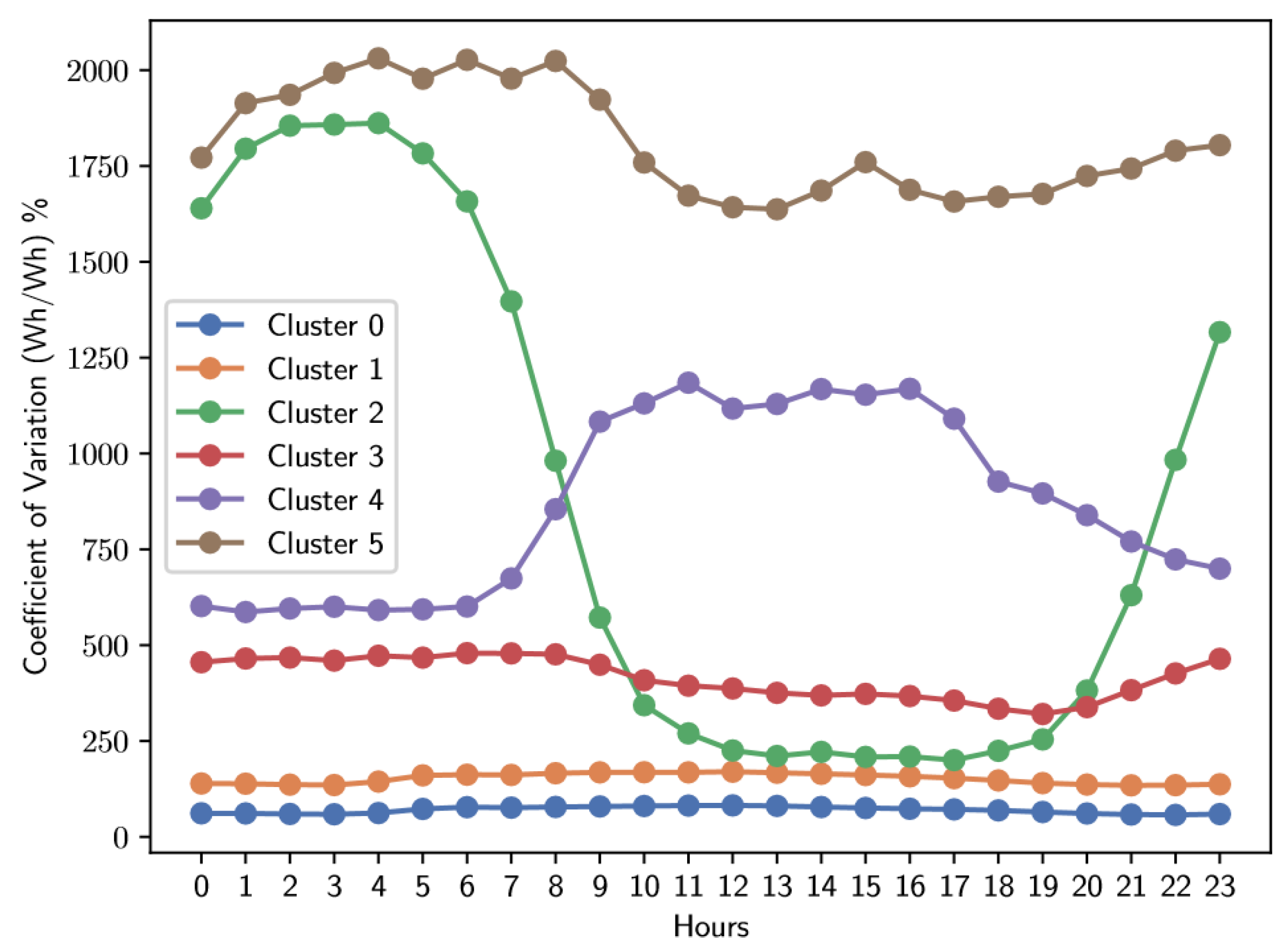

Table 1.
Number of users per cluster for the Weekday type.
| Cluster | 0 | 1 | 2 | 3 | 4 | 5 |
| Number of Users | 32826 | 9762 | 253 | 1220 | 367 | 146 |
| Average CV0−23 | 70.17 | 152.37 | 878.46 | 415.48 | 866.97 | 1811.93 |
Figure 8.
Average coefficient of variation of electrical energy consumption for the Weekday type.
Saturday
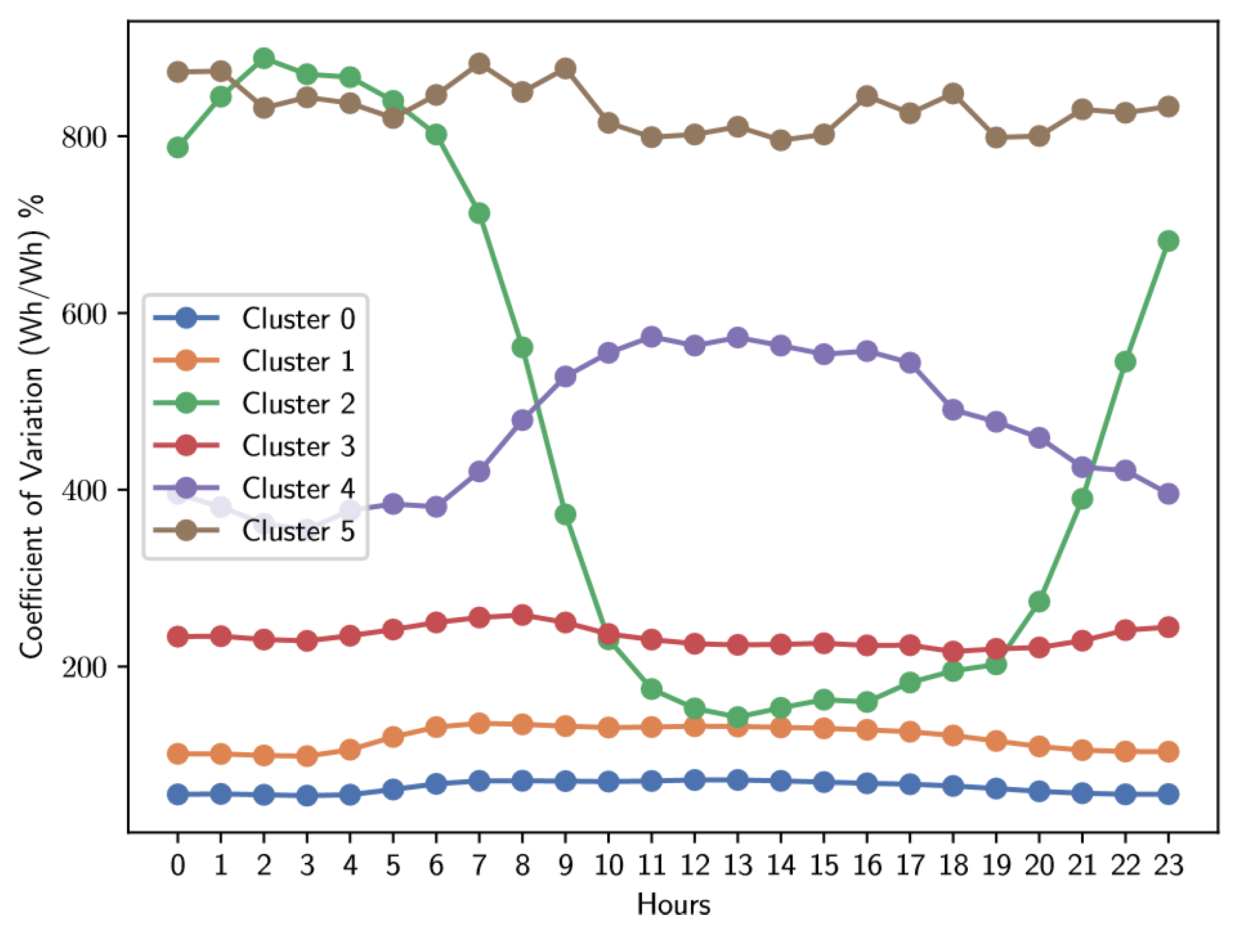
Table 2.
Number of users per cluster for the Saturday type.
| Cluster | 0 | 1 | 2 | 3 | 4 | 5 |
| Number of Users | 26087 | 14637 | 315 | 2565 | 673 | 252 |
| Average CV0−23 | 63.71 | 119.45 | 466.33 | 233.78 | 467.18 | 832.06 |
Figure 9.
Average coefficient of variation of electrical energy consumption for the Saturday type.
Sunday-Holiday
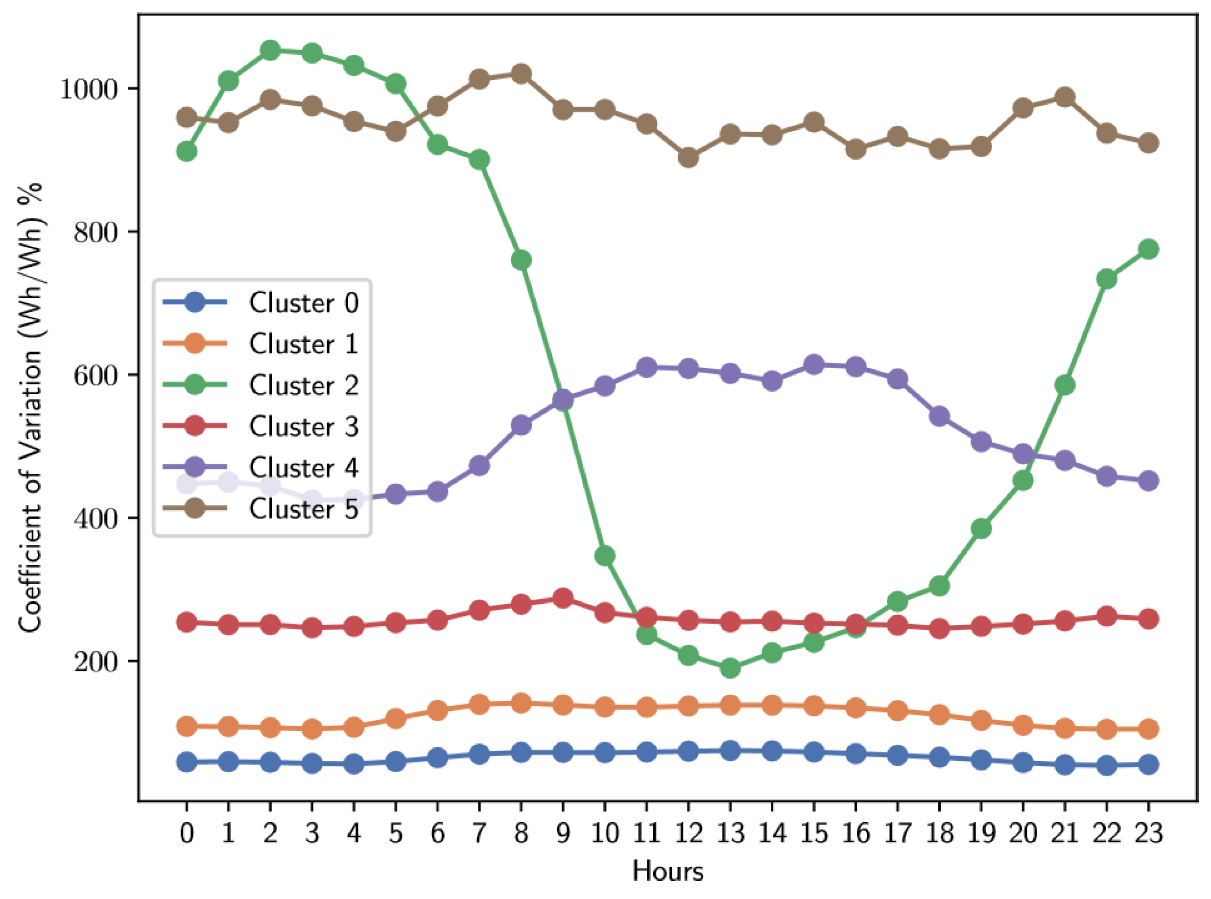
Table 3.
Number of users per cluster for the Sunday-Holiday type.
| Cluster | 0 | 1 | 2 | 3 | 4 | 5 |
| Number of Users | 26866 | 14179 | 220 | 2335 | 654 | 262 |
| Average CV0−23 | 65.08 | 123.54 | 599.97 | 257.31 | 515.71 | 954.16 |
Figure 10.
Average standard deviations of electrical energy consumption for the Sunday-Holiday type.
Figure 10.
Average standard deviations of electrical energy consumption for the Sunday-Holiday type.
Table 4.
Association rules by day type.
| Day Type | Antecedent | Consequent | Support | Confidence | |
|---|---|---|---|---|---|
| Weekday | ’socio eco level 3’, ’cold climate’, ’regulated residential user’ | cluster label | 0 | 0.40 | 0.77 |
| ’socio eco level 2’, ’cold climate’, ’regulated residential user’ | cluster label | 0 | 0.15 | 0.69 | |
| Saturday | ’socio eco level 3’, ’cold climate’, ’regulated residential user’ | cluster label | 0 | 0.32 | 0.62 |
| ’socio eco level 2’, ’cold climate’, ’regulated residential user’ | cluster label | 0 | 0.11 | 0.50 | |
| Sunday | ’socio eco level 3’, ’cold climate’, ’regulated residential user’ | cluster label | 0 | 0.33 | 0.64 |
| ’socio eco level 2’, ’cold climate’, ’regulated residential user’ | cluster label | 0 | 0.11 | 0.51 | |
5.5. Clustering by the coefficient of variation
From the filtered data (excluding users with low variability), the K-means clustering technique was reapplied, which resulted in the distinction of six different clusters for each day category.
Graphs illustrating the average coefficient of variation corresponding to each cluster, classified according to the type of day, are shown below. These graphs are supported by detailed information on the characteristics of each group.
Weekday
This subsection details the results of clustering the variability of electricity consumption during Weekday.
Analysis of Figure 11 and Table 5 and Table 6 reveals interesting patterns in the distribution of users among the clusters. It is notable that clusters 0 and 1 accommodate the largest number of users. In particular, cluster 0 is characterized by a coefficient of variation that remains constant throughout the day, averaging around 150%. In contrast, the behavior in cluster 1 is significantly different: it shows pronounced variability during the morning hours, from dawn to about 10 a.m. Subsequently, its coefficient of variation stabilizes and remains constant until 20 hours, when there is a new increase in variability.
Saturday
This subsection presents the results of the clustering applied to the variability of electricity energy consumption on Saturday.
Analysis of Figure 12 and Table 7 and Table 8 reveals that the majority of users are concentrated in clusters 0 and 1. In cluster 0, there is a relatively constant coefficient of variation, although with a slight increase in the early morning hours, specifically around 4 a.m., and a slight decrease in the afternoon, around 6 p.m., with an average of 119%. In contrast, cluster 1 also shows a fairly stable coefficient of variation throughout the day, but with a significantly higher average: approximately 226%.
Sunday-Holiday
This subsection presents the results of applying clustering techniques to the variability of electricity consumption on days categorized as Sunday-Holiday.
Analysis of Figure 13 and Table 9 and Table 10 reveals that most users are concentrated primarily in clusters 0 and 2. It is notable that cluster 0, which contains the largest number of users, has a coefficient of variation that remains constant throughout the day, hovering at 123%. In contrast, the coefficient of variation for cluster 2 is around 253%. It is important to note that the consumption patterns observed on Saturdays and Sundays show a remarkable similarity.
5.6. Selection of Clusters and Analysis of Time Intervals
According to the obtained results, most users are grouped in clusters 0, followed by those of cluster 1 for Weekday and Saturday types. For Sunday and Holiday types, clusters 0 and 2 prevail. To better understand the behavior of these groups, which contain a larger number of users, a box plot was developed for each cluster. To compare the coefficient of variation for different types of days and clusters, an additional line in each diagram was graphed, which has a value of 1.2 times the average electricity consumption relative to the standard deviation of users’ electricity consumption. This graphical representation facilitates the identification of patterns and anomalies in the variability of consumption, and provides a visual reference for assessing the dispersion of data in relation to the mean.
Weekday
Analysis of the box plot in Figure 14 for cluster 0 reveals an interesting dynamic in the variability of consumption. There is a notable increase in variability between 5 and 7 hours. Subsequently, this variability decreases and remains stable until approximately 18 hours; at that point, it begins to decrease steadily. Despite these changes, the average coefficient of variation remains above 150%.
Figure 15 shows that in cluster 1, the variability is quite constant during the morning and continues until noon. There is a slight increase in variability around noon, followed by a decrease in the afternoon. From 18 hours, there is a slight increase, which intensifies between 21 and 23 hours. It is important to note that the average variation in cluster 1 is significantly higher than that of cluster 0.
Saturday
For clusters 0 and 1, which encompass the largest number of users, a detailed analysis was performed with box plots; Figure 16 and Figure 17, respectively, show their results. The analysis of Figure 16, corresponding to cluster 0, shows that the coefficient of variation experiences a notable increase between 6 and 7 hours, followed by a slight decrease and a period of stability until approximately 17 hours, when there is a slight decreasing trend during the night. In contrast, Figure 17, representing cluster one, indicates that the coefficient of variation remains relatively constant throughout the day, but there are slight increases between 6 and 9 hours.
Sunday-Holiday
Figure 18 and Figure 19 show the box plots for clusters 0 and 2, which have the largest number of users. For cluster 0, there is an increase in the coefficient of variation from 6 to about 8 hours, followed by a period of stability until noon. In the afternoon, specifically from 12 to 15 hours, there is a slight peak in variability, which then gradually decreases until 17 hours. Figure 19 corresponding to cluster 2, shows a different pattern. In this case, the coefficient of variation remains constant, with a slight increase between 6 and 8 hours. Subsequently, it remains stable until the night, when there is a significant increase in variability from 19 to 23 hours.
5.7. Generation of Association Rules and Classification
Table 11 shows the association rules generated by the Apriori algorithm, applied to different types of days from the filtered dataset, which excludes users with low variability removed in previous stages of the methodology. Interestingly, all the resulting rules indicate that the users belong to cluster 0, which contains the majority of users for each type of day. Predominantly, these users are in socioeconomic strata 2 and 3 and are residential type. Contrasting these rules with those obtained before removing users with higher variability (see Table 4), in which the antecedents were also residential users from strata 2 and 3, shows that the variability of consumption or the coefficient of variation of electrical energy is not directly related to exogenous variables such as climate, socioeconomic level, or type of user. This suggests that users with the mentioned characteristics can have both low and high variability in their electricity consumption.
5.8. Determination of Time-of-Use Tariff Intervals
The analysis performed in the previous stages of this methodology reveals that certain time intervals have remarkable flexibility in energy consumption. This conclusion is based on the box plots in Figures 14 to 19, which illustrate the coefficient of variation for the clusters with the largest number of users. During weekdays and Saturdays, the most representative cluster is cluster 1, while on Sundays and holidays, it is cluster 2. The average coefficient of variation of both clusters are above 120%; this suggests a considerable ability of these users to adapt to various time-based tariff schemes. In contrast, users belonging to cluster 0have a coefficient of variation below 120% for all types of days and at certain times.
- On Weekdays, it is observed that the coefficient of variation exceeds 120% from 5 to 18 hours, with a notable peak between 5 and 7 hours.
- On Saturdays, the coefficient of variation remains above 120% from 6 to 17 hours, with a peak between 6 and 7 hours.
- On Sundays-Holidays, the coefficient of variation exceeds 120% from 6 to 17 hours, with a significant increase between 6 and 9 hours and a slight increase from 19 to 23 hours.
However, it is crucial to integrate this information with the financial and generation data of the network operator. This combination will make it possible to identify time intervals that not only promote savings and energy efficiency for consumers, but also optimize the operational and economic benefits for electricity companies. The implementation of differentiated tariffs in these time intervals could lead to more balanced and sustainable energy consumption as well as more efficient operation of the electrical grid.
6. Conclusions
The methodology developed in this study successfully identifies optimal time intervals for implementing differential tariff schemes based on the variability of electricity consumption. This approach was validated through a case study, which identified specific intervals for weekdays (5 to 6 hours, with a peak between 5 and 7 hours), Saturdays (6 to 5, with a peak between 6 and 7 hours), and Sundays-holidays (6 hours to 5 hours, with peaks between 6 and 9 hours and 19 to 23 hours).
The findings indicate that the early morning hours, specifically between 6 and 9 hours, are the most suitable for implementing Time-of-Use tariffs across all types of days due to high variability peaks observed in these intervals for clusters with a majority of users. Sundays-holidays have a consumption pattern similar to Saturdays regarding electricity variability, differing only in the exact timing of the variability peak. This similarity suggests the potential feasibility of simply categorizing days as weekdays and non-weekdays in future studies.
The study also attempted to correlate exogenous variables such as socioeconomic level, type of user, climate, and city with variability of electricity consumption. However, no direct relationship was found between variability of consumption and these exogenous factors. Users of lower socioeconomic levels and residing in colder climates, such as Bogota, had both low and high variability, possibly influenced by the imbalance of the dataset, in which records from Bogota’s working-class residents predominate. Therefore, it is recommended that this methodology be applied to more balanced datasets covering diverse user profiles is recommended for further validation.
It is noteworthy that approximately 60-73% of users, for each type of day, have low variability of around 70% in their coefficient of variation. These users were excluded from the differential tariff analysis due to their potentially low flexibility in consumption patterns.
This methodology is intended as a complementary tool in the formulation of differential tariff schemes. For its effective implementation, additional information, such as financial and generation data from network operators, should be considered. This approach aims not only to promote savings and enhance efficiency for consumers, but also to optimize operational management of electricity companies.
7. Future Work
For future research, it is proposed that the relationship between the flexibility and variability of electricity consumption be explored. This will testing with real users under differential tariffs to study their responses. Additionally, the methodology could be adjusted to integrate both the variability and the total volume of energy consumption. This would make it possible to identify temporal intervals and to apply association rules with the aim of discovering possible links between actual consumption and external variables. Another possible adjustment is to modify the methodology for the classification to be independent of the type of day.
Since this study did not establish a conclusive relationship between the variability of electricity consumption and the exogenous variables mentioned, a future line of research could involve exploring with different exogenous variables. This would help to determine whether the lack of correlation observed is specific to the dataset used or whether it is a more general trend.
Author Contributions
Conceptualization, J.R.G. and O. D.; Methodology, J.R.G. and J.D.A.; investigation, J.D.A.; writing—original draft preparation, O.D.; writing—review and editing, J.D.A. and J.R.G.; funding acquisition, J.R.G. All authors have read and agreed to the published version of the manuscript.
Funding
This research was supported by “Project microgrids: energía flexible y eficiente para Cundinamarca. BPIN: 2021000100523, Convenio Especial de Cooperación No. SCTEI-CDCCO-123-2022 Suscrito Entre El Departamento de Cundinamarca- Secretaria De Ciencia, Tecnología e Innovación y la Universidad Nacional de Colombia y la Universidad de Cundinamarca”.
Data Availability Statement
Additional data are available on request by contacting the corresponding author of this manuscript.
Conflicts of Interest
The authors declare that there is no conflict of interest regarding the publication of this paper.
References
- Naciones Unidas, “Protocolo de Kioto de la convención marco de las naciones unidas sobre el cambio climático” 12 1998.
- C. M. de las Naciones Unidas sobre el Cambio Climático, “Acuerdo de París” 12 2015.
- Comisión Europea, “Una transición hacia una energía limpia,” 7 2022. [Online]. Available: https://commission.europa.eu/strategy-and-policy/priorities-2019-2024/european-green-deal/energy-andgreen-deal_es. 2019.
- D. N. de Planeación, M. del Trabajo, M. de Minas y Energía, M. de Comercio Industria y Turismo, M. de Ambiente y Desarrollo Sostenible, M. de Transporte, and M. de Ciencia Tecnología e Innovación, “Documento CONPES 4075 - política de transición energética,” 3 2022.
- M. Aro, K. Piira, and K. Maki, “Business model for household flexibility - a case study,” 9 2021, pp. 20–23.
- Enel X, “¿cómo funciona la respuesta a la demanda y por qué es importante?” [Online]. Available: https://corporate.enelx.com/es/question-and-answers/what-is-demand-response-how-does-it-work.
- Z. Chen, A. M. Amani, X. Yu, and M. Jalili, “Control and optimization of power grids using smart meter data: A review,” Sensors, 2023, 23, 2.
- J. S. Guerrero-Prado, W. Alfonso-Morales, and E. F. Caicedo-Bravo, “A data analytics/big data framework for advanced metering infrastructure data,” Sensors, 2023, 21, 8.
- S. Gao, T. E. Song, S. Liu, C. Zhou, C. Xu, H. Guo, X. Li, Z. Li, Y. Liu, W. Jiang, J. Wang, and S. Wang, “Joint optimization of planning and operation in multi-region integrated energy systems considering flexible demand response,” IEEE Access, 2021, 9, 75840–75863.
- J. Z. Bebic, I. M. Berry, A. N. James, and D. O. Lee, “Quantifying electric load flexibility using smart meter data” 2019.
- A. Fraija, K. Agbossou, N. Henao, S. Kelouwani, M. Fournier, and S. S. Hosseini, “A discount-based time-of-use electricity pricing strategy for demand response with minimum information using reinforcement learning,” IEEE Access, 2022, 10, 54018–54028. [Google Scholar] [CrossRef]
- M. E. Honarmand, V. Hosseinnezhad, B. Hayes, M. Shafie-Khah, and P. Siano, “An overview of demand response: From its origins to the smart energy community,” IEEE Access, 2021, 9, 96851–96876. [CrossRef]
- F. de Ciencias F´ısicas y Matemáticas Universidad de Chile Centro de la Energía, S. E. Nacional, R. Palma, M. Matus, R. Torres, C. Benavides, E. Sierra, R. Sepulveda, and F. Riquelme, “Concepto´ de flexibilidad en el sistema eléctrico nacional,” 2019. [Online]. Available: www.centroenergia.cl.
- M. B. Awan and Z. Ma, “Building energy flexibility: definitions, sources, indicators, and quantification methods,” pp. 17–40, 2023.
- Comisión de Regulación de Energía y Gas, “Respuesta de la demanda en el sistema interconectado nacional -hoja de ruta-documento de consulta pública,” 1 2022.
- P. A. Schirmer and I. Mporas, “Non-intrusive load monitoring: A review,” IEEE Transactions on Smart Grid, 2023, 14, 769–784. [CrossRef]
- Y. Tao, J. Qiu, S. Lai, Y. Wang, and X. Sun, “Reserve evaluation and energy management of micro-grids in joint electricity markets based on non-intrusive load monitoring,” IEEE Transactions on Industry Applications, 2023, 59, 207–219. [CrossRef]
- L. Liu, F. Li, Z. Cheng, Y. Zhou, J. Shen, R. Li, and S. Xiong, “Nonintrusive load monitoring method considering the time-segmented state probability,” IEEE Access, 2022, 10, 39627–39637. [CrossRef]
- S. Welikala, C. Dinesh, M. P. B. Ekanayake, R. I. Godaliyadda, and J. Ekanayake, “Incorporating appliance usage patterns for nonintrusive load monitoring and load forecasting,” IEEE Transactions on Smart Grid, 2019, 10, 448–461. [CrossRef]
- A. Nawaz, G. Hafeez, I. Khan, K. U. Jan, H. Li, S. A. Khan, and Z. Wadud, “An intelligent integrated approach for efficient demand side management with forecaster and advanced metering infrastructure frameworks in smart grid,” IEEE Access, 2020, 8, 132551–132581. [Google Scholar] [CrossRef]
- B. Canizes, B. Mota, P. Ribeiro, and Z. Vale, “Demand response driven by distribution network voltage limit violation: A genetic algorithm approach for load shifting,” IEEE Access, 2022, 10, 62183–62193. [Google Scholar] [CrossRef]
Figure 1.
Graphic Representation of the Stages of the Proposed Methodology.
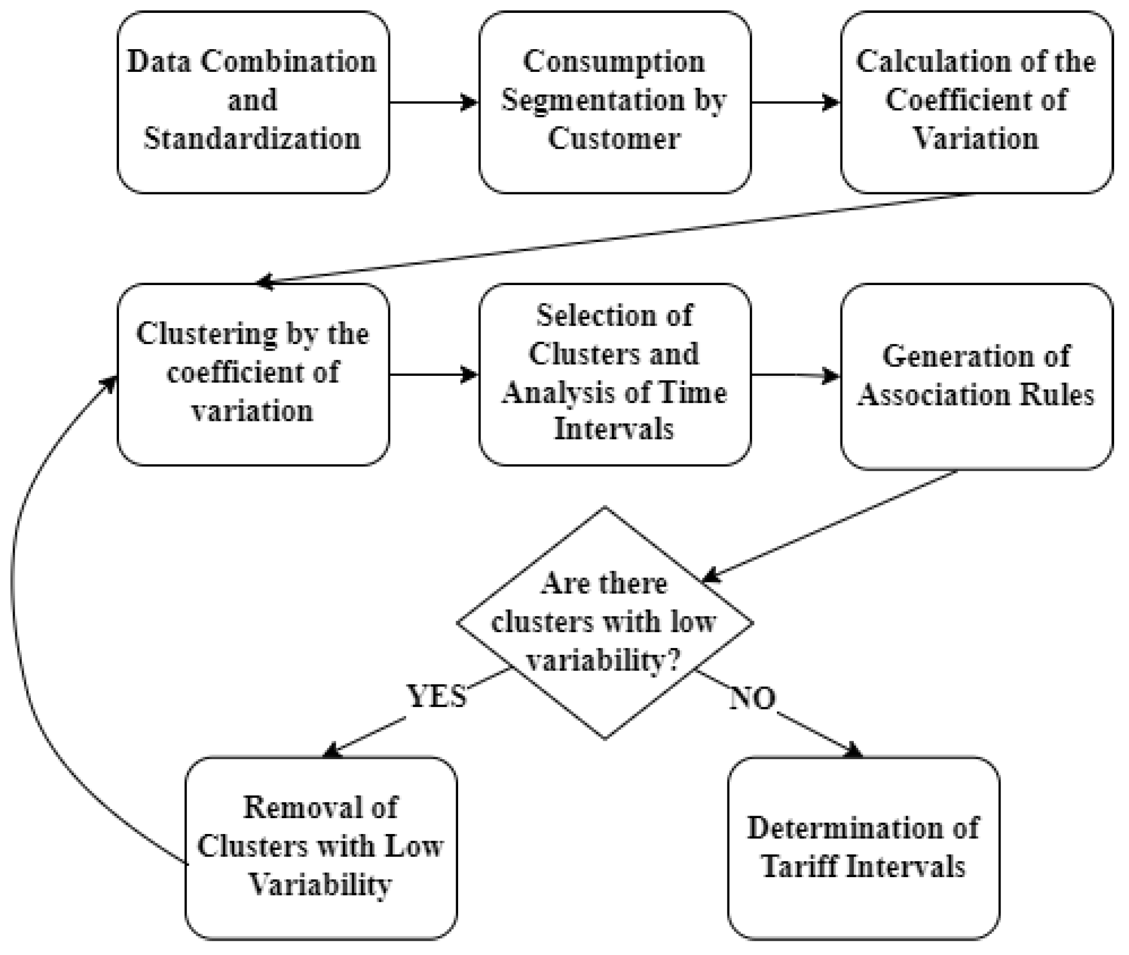
Figure 2.
Data Combination and Standardization.
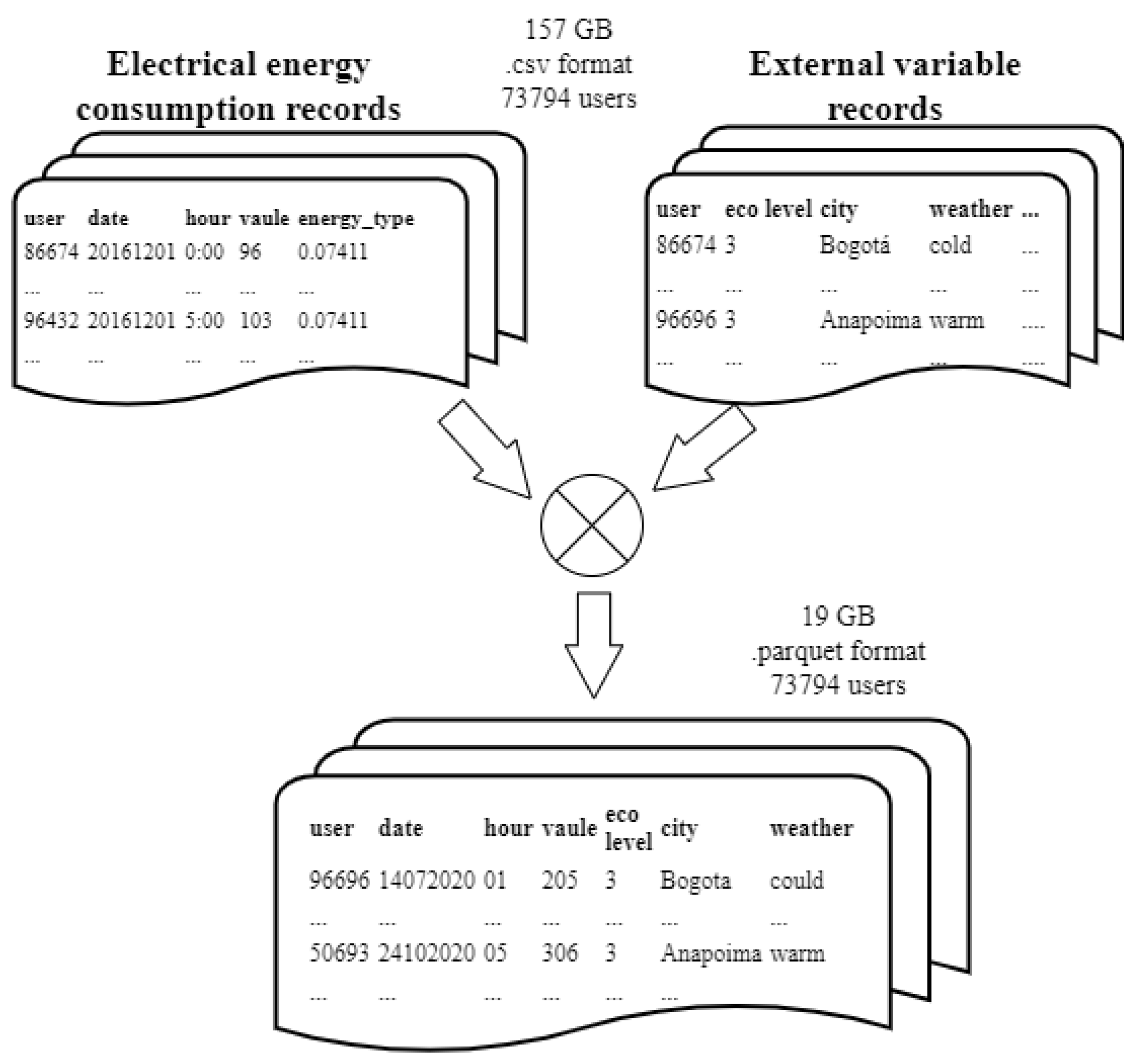
Figure 3.
Consumption Segmentation by Customer.
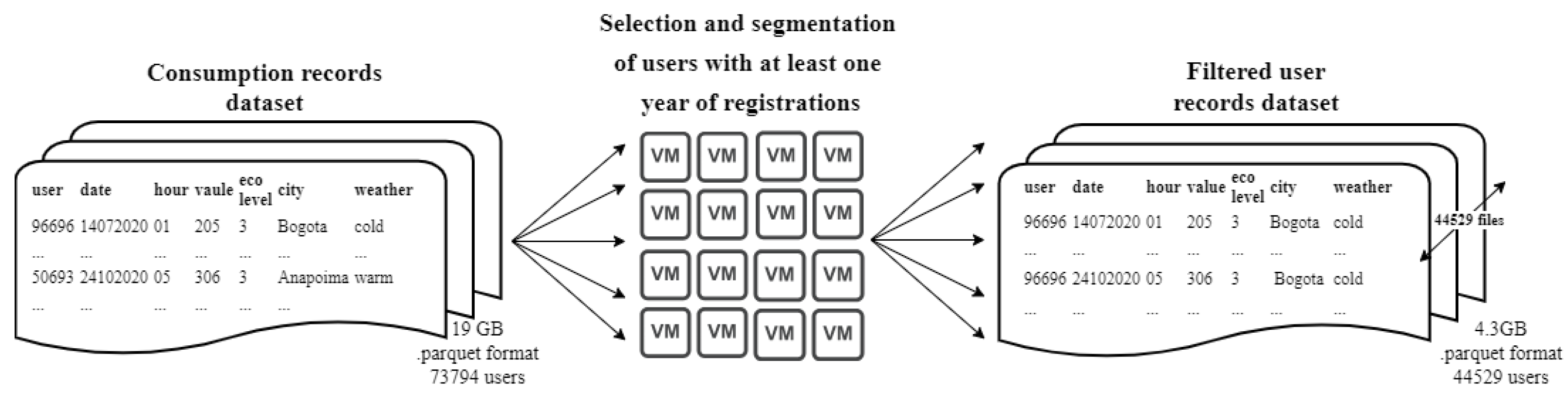
Figure 4.
Calculation of the Coefficient of Variation.
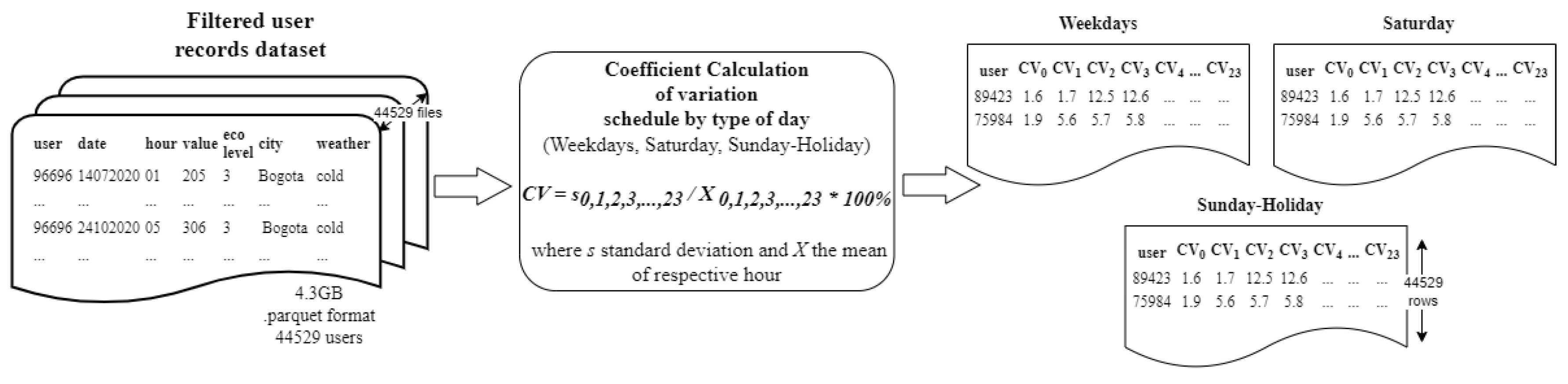
Figure 5.
Clustering by the coefficient of variation.
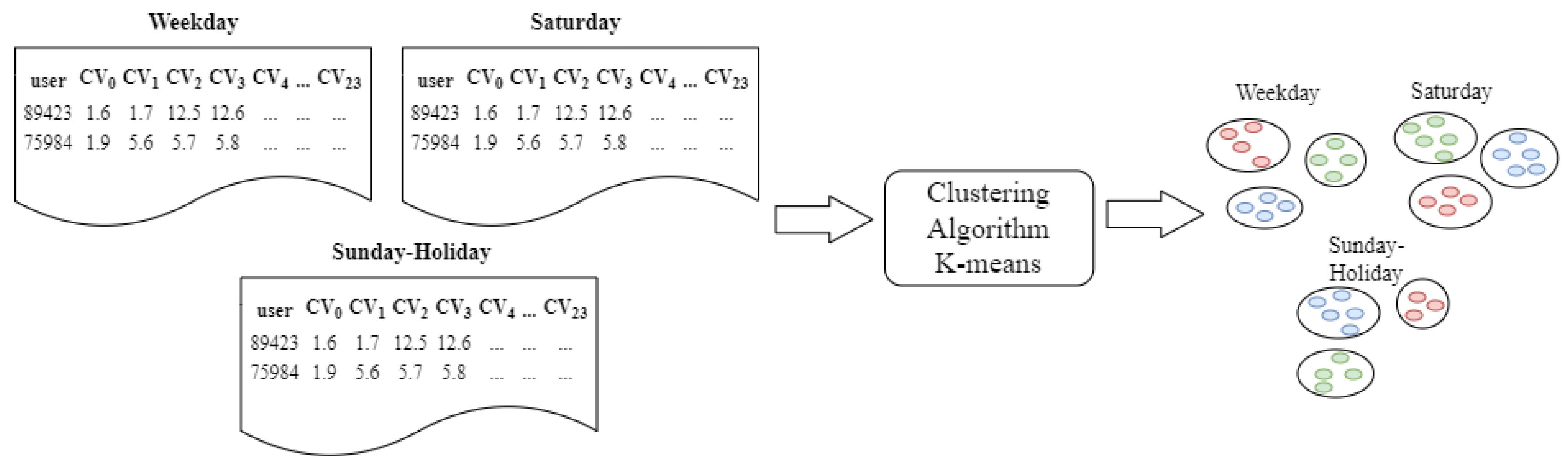
Figure 6.
Generation of Association Rules and Classification.
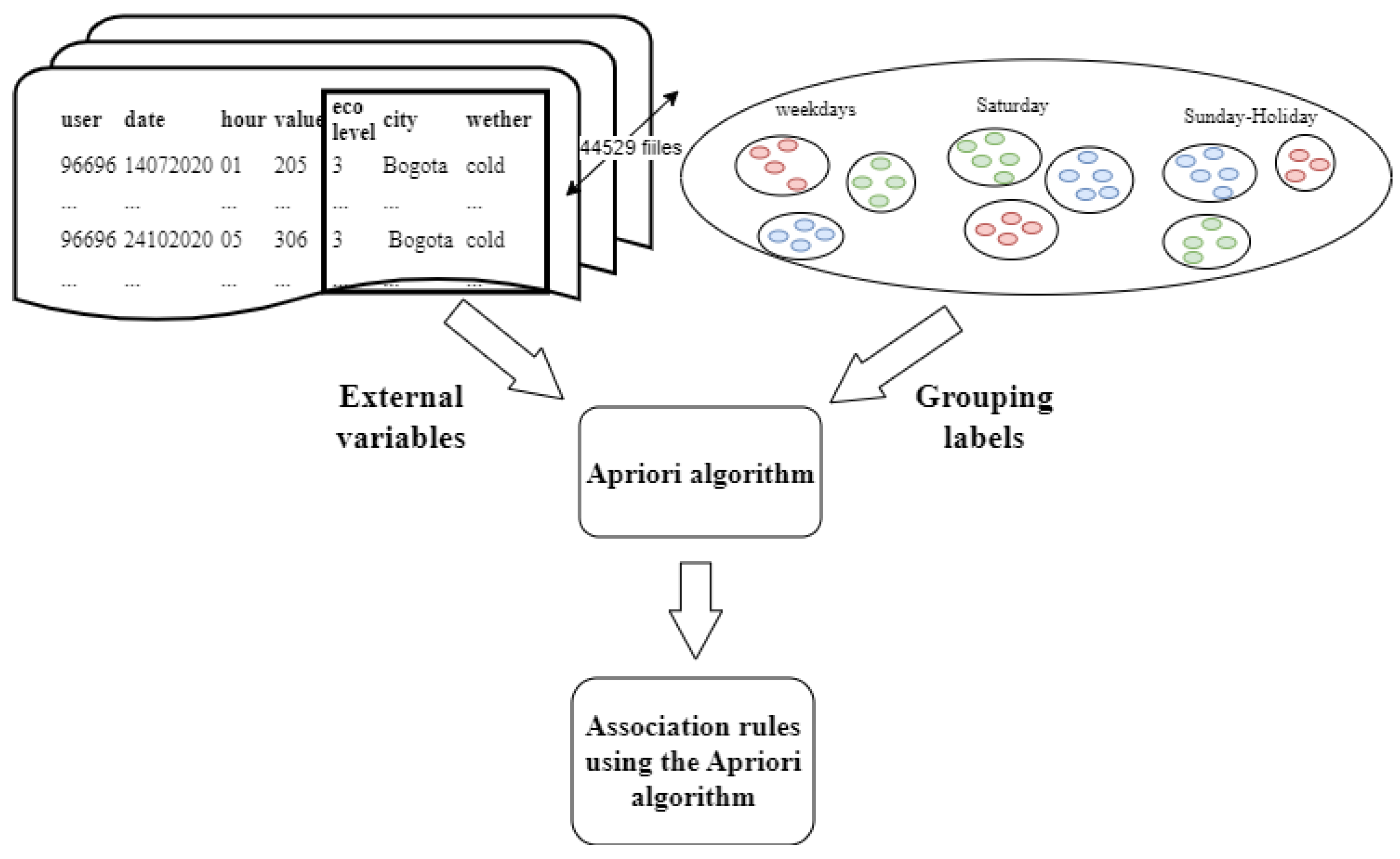
Figure 7.
Data Pre-processing.
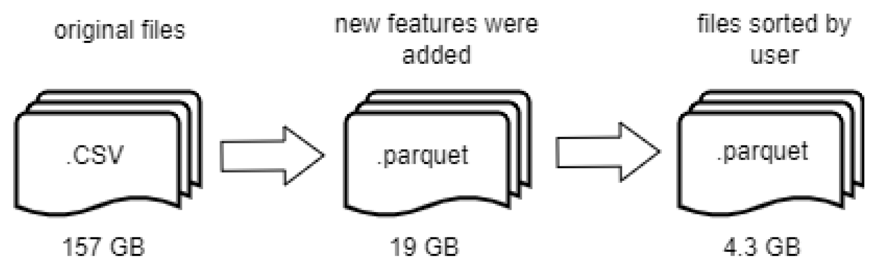
Figure 11.
Average coefficient of variation of electrical energy consumption for Weekday.
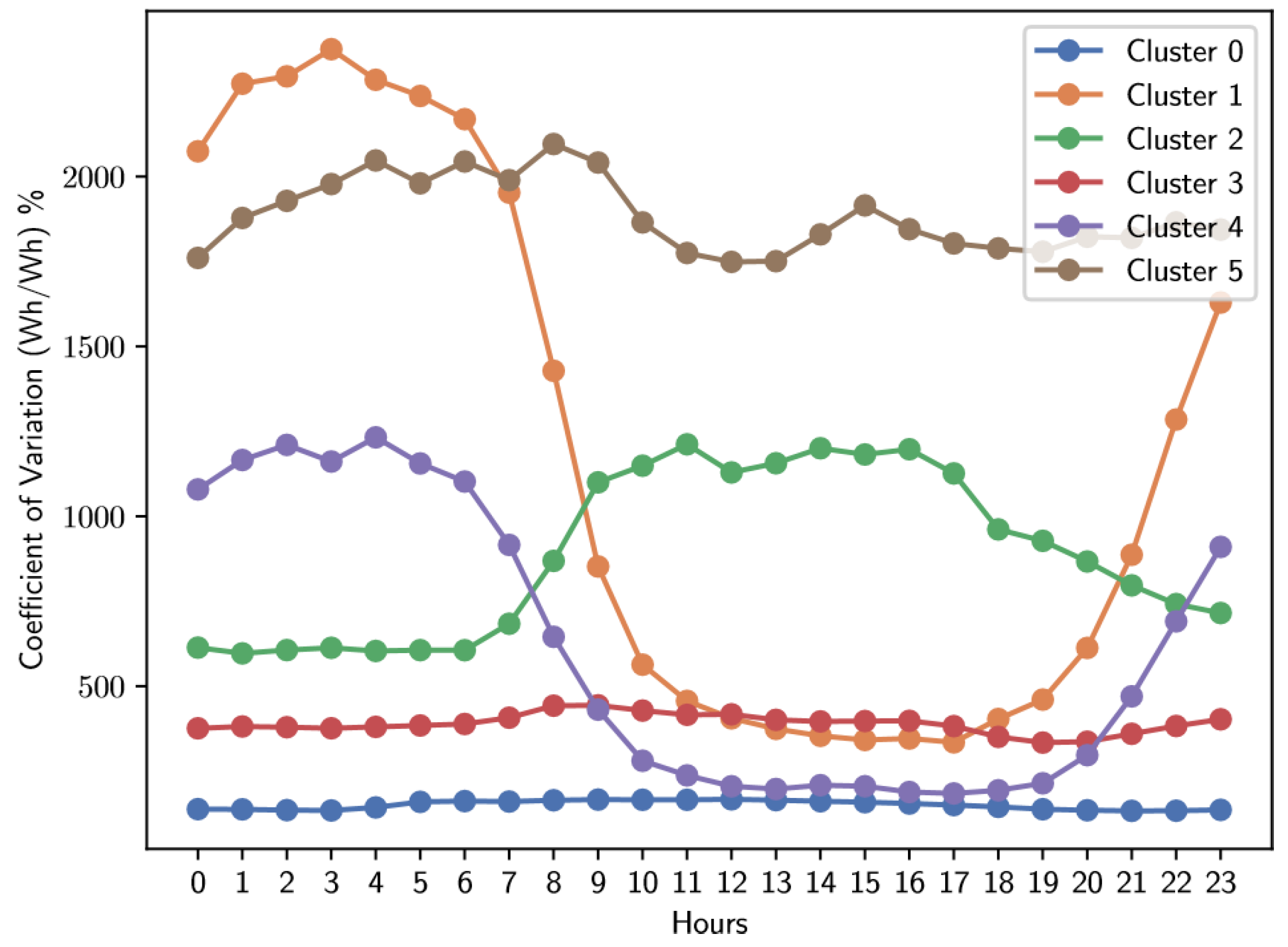
Figure 12.
Average coefficient of variation of electrical energy consumption for Saturday.
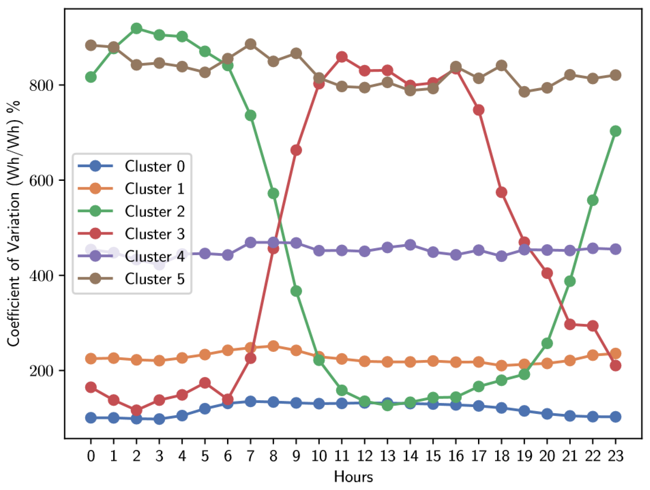
Figure 13.
Average standard deviation of electrical energy consumption for Sunday-Holiday.
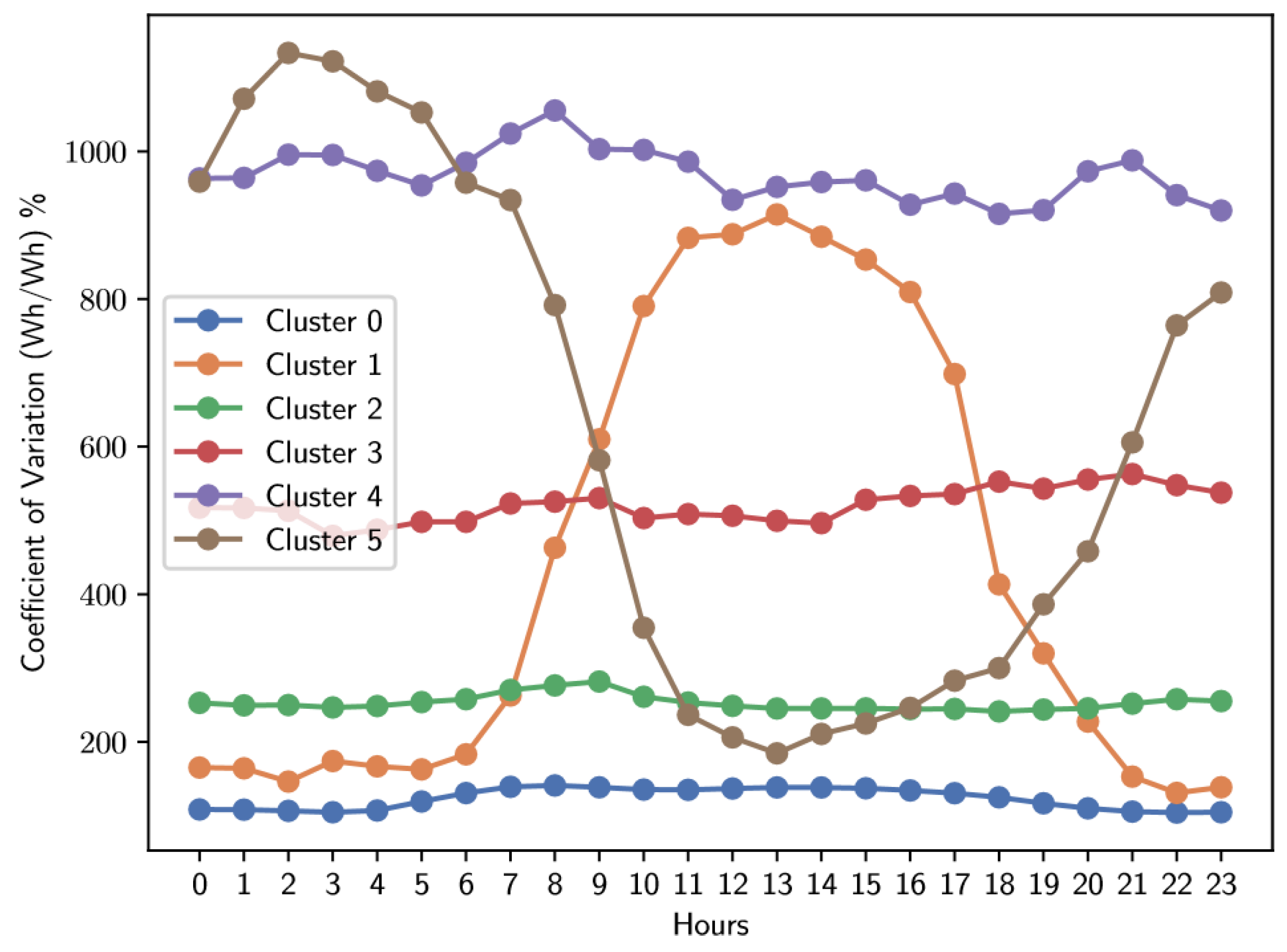
Figure 14.
Box plot for cluster 0 for the Weekday type.
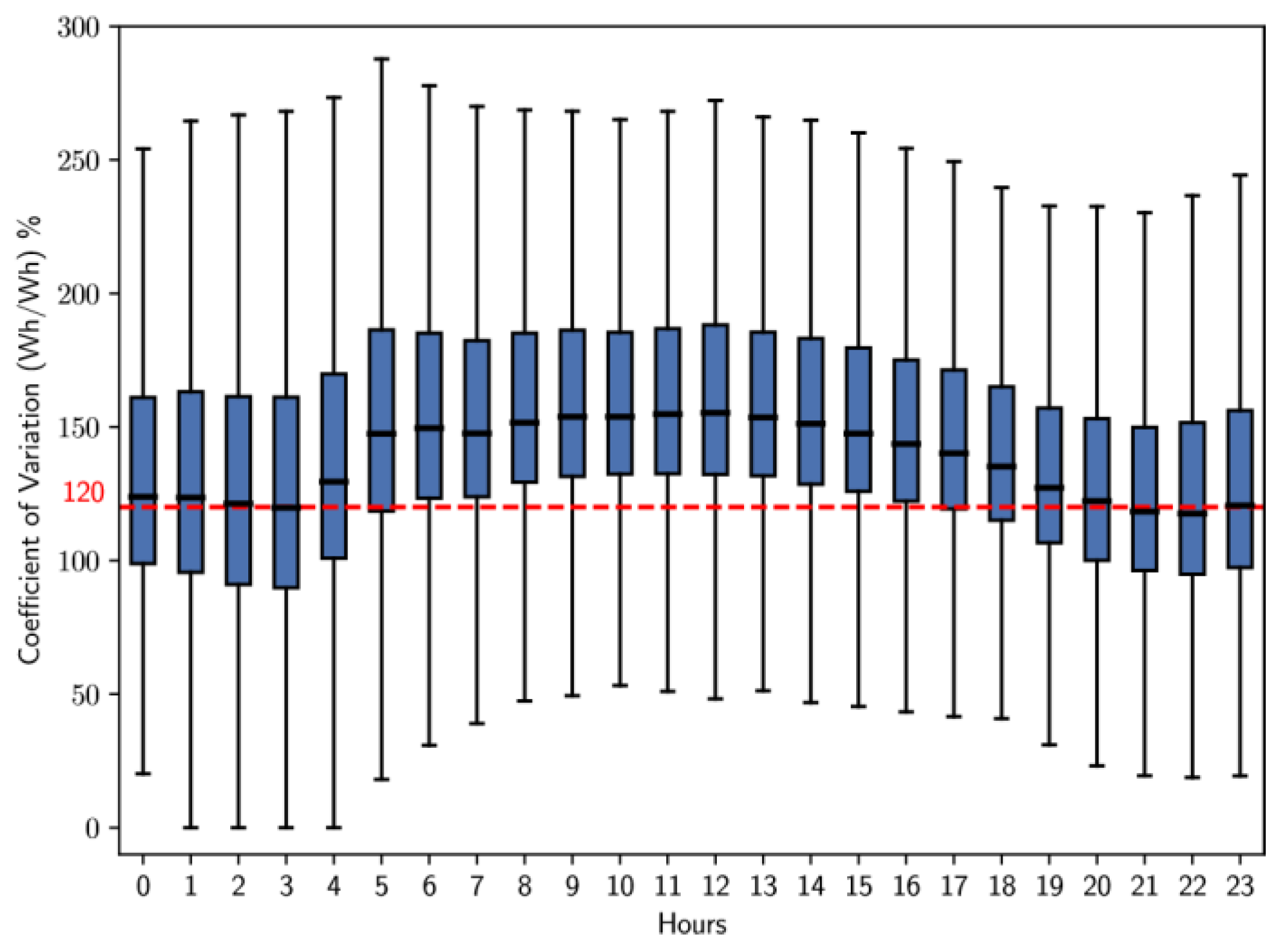
Figure 15.
Box plot for cluster 1 for the Weekday type.
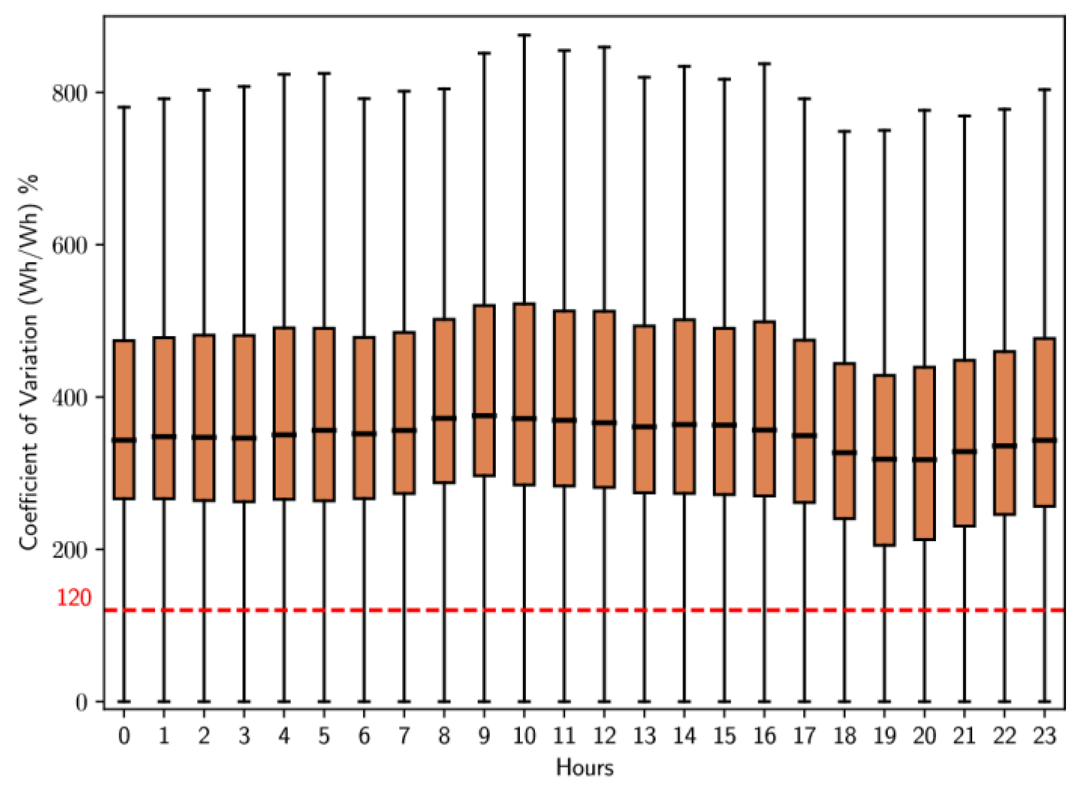
Figure 16.
Box plot for cluster 0 for the Saturday type.
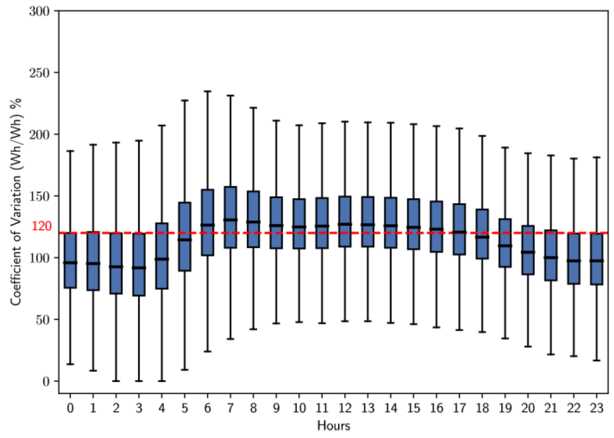
Figure 17.
Box plot for cluster 1 for the Saturday type.
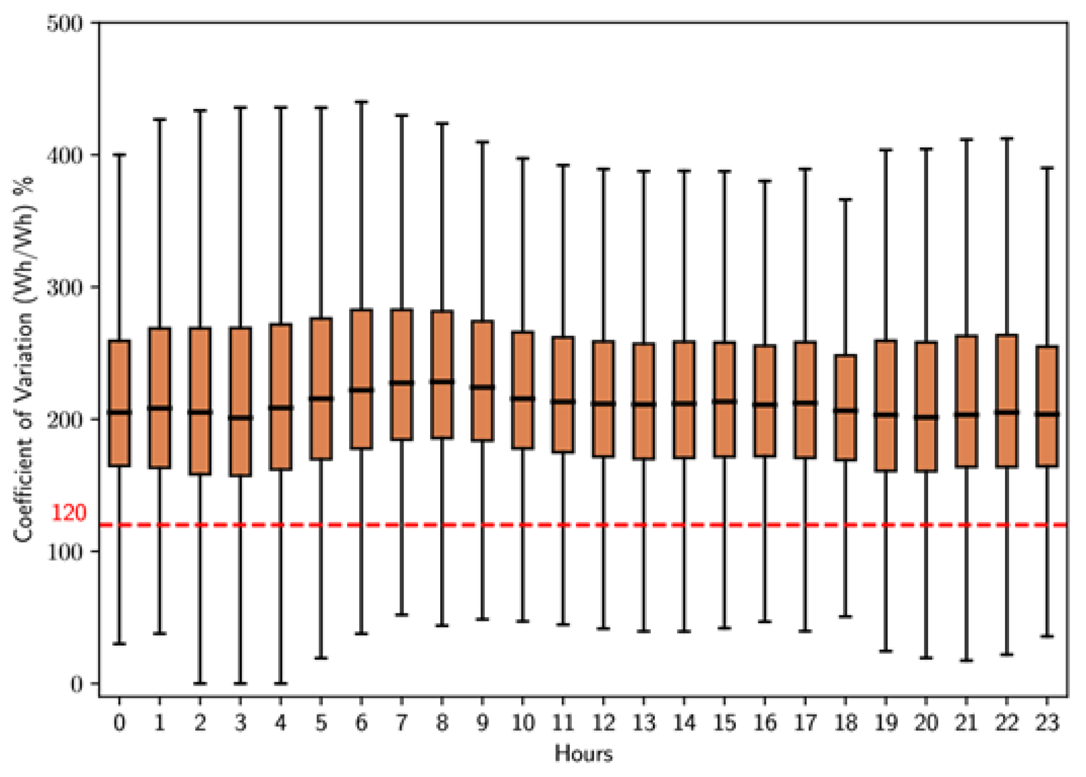
Figure 18.
Box plot for cluster 0 for the Sunday-Holiday type.
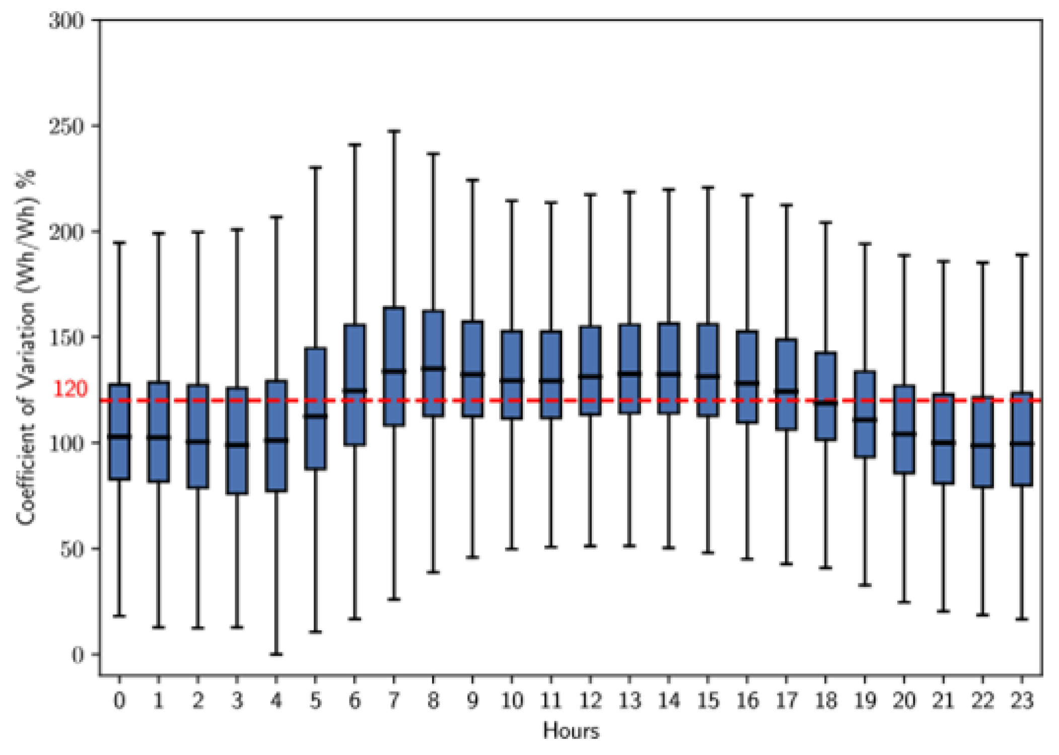
Figure 19.
Box plot for cluster 2 for the Sunday-Holiday type.
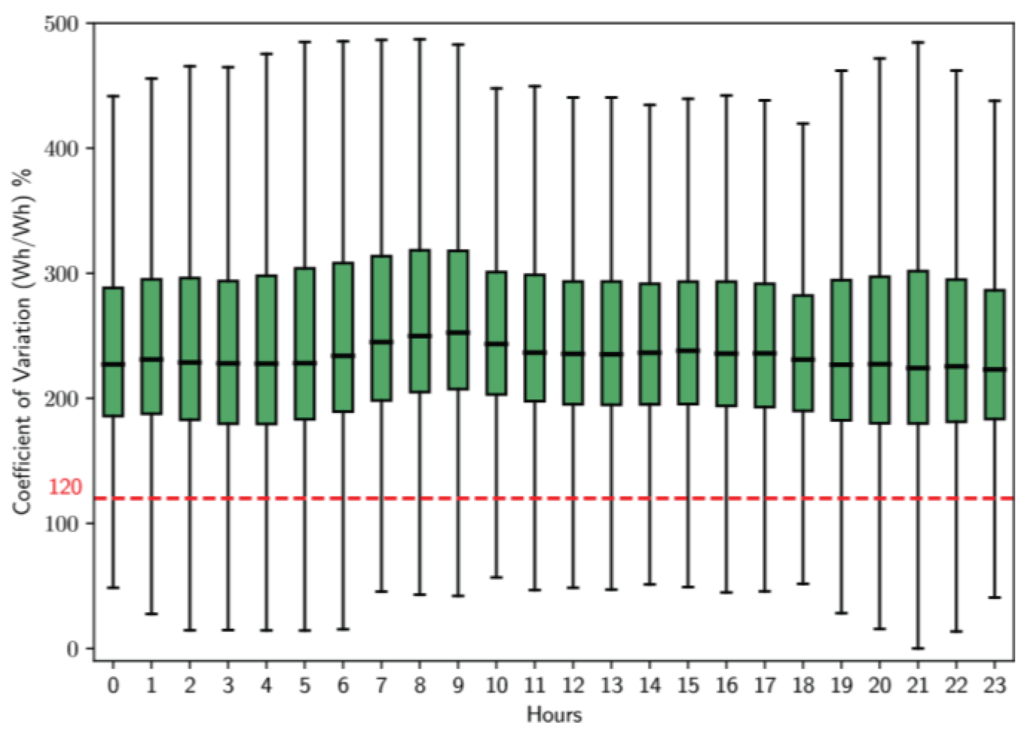
Table 5.
Cluster information for weekday by socioeconomic level.
| Cluster | Number of Users | Socioeconomic Level | |||||
|---|---|---|---|---|---|---|---|
| 0 | 1 | 2 3 | 4 | 5 | 6 | ||
| 0 | 9604 | 734 | 818 | 2673 4539 | 561 | 214 | 65 |
| 1 | 1243 | 222 | 79 | 263 532 | 123 | 12 | 12 |
| 2 | 348 | 27 | 23 | 57 177 | 58 | 5 | 1 |
| 3 | 305 | 208 | 5 | 34 55 | 1 | 0 | 2 |
| 4 | 127 | 84 | 5 | 9 28 | 1 | 0 | 0 |
| 5 | 121 | 24 | 5 | 26 57 | 7 | 0 | 2 |
Table 6.
Cluster information for weekday by user type.
| Cluster | User Type | |||
|---|---|---|---|---|
| official | residential | industrial | commercial | |
| 0 | 4 | 8870 | 68 | 662 |
| 1 | 2 | 1021 | 22 | 198 |
| 2 | 1 | 321 | 1 | 25 |
| 3 | 0 | 97 | 26 | 182 |
| 4 | 0 | 43 | 3 | 81 |
| 5 | 1 | 97 | 0 | 23 |
Table 7.
Cluster information for Saturday by socioeconomic level.
| Cluster | Number of Users | Socioeconomic Level | |||||
|---|---|---|---|---|---|---|---|
| 0 | 1 | 2 3 | 4 | 5 | 6 | ||
| 0 | 14455 | 643 | 1186 | 4046 7330 | 884 | 299 | 67 |
| 1 | 2666 | 482 | 177 | 613 1110 | 205 | 59 | 20 |
| 2 | 276 | 212 | 5 | 18 41 | 0 | 0 | 0 |
| 3 | 161 | 20 | 10 | 17 87 | 25 | 1 | 1 |
| 4 | 631 | 81 | 46 | 128 301 | 59 | 9 | 7 |
| 5 | 253 | 43 | 16 | 55 112 | 21 | 0 | 6 |
Table 8.
cluster information for Saturday by user type.
| Cluster | User Type | |||
|---|---|---|---|---|
| official | residential | industrial | commercial | |
| 0 | 5 | 13812 | 54 | 584 |
| 1 | 2 | 2184 | 54 | 426 |
| 2 | 0 | 64 | 26 | 186 |
| 3 | 0 | 141 | 0 | 20 |
| 4 | 0 | 550 | 8 | 73 |
| 5 | 1 | 210 | 2 | 40 |
Table 9.
Cluster information for Sunday-Holiday by socioeconomic level.
| Cluster | Number of Users | Socioeconomic Level | |||||
|---|---|---|---|---|---|---|---|
| 0 | 1 | 2 3 | 4 | 5 | 6 | ||
| 0 | 14114 | 691 | 1173 | 4066 6947 | 865 | 298 | 74 |
| 1 | 154 | 40 | 8 | 15 65 | 26 | 0 | 0 |
| 2 | 2336 | 469 | 145 | 521 962 | 182 | 45 | 12 |
| 3 | 612 | 154 | 40 | 108 257 | 40 | 6 | 7 |
| 4 | 243 | 69 | 16 | 41 96 | 16 | 0 | 5 |
| 5 | 191 | 142 | 2 | 19 27 | 1 | 0 | 0 |
Table 10.
cluster information for Sunday-Holiday by user type.
| Cluster | User Type | |||
|---|---|---|---|---|
| official | residential | industrial | commercial | |
| 0 | 5 | 13423 | 61 | 625 |
| 1 | 0 | 114 | 1 | 39 |
| 2 | 3 | 1867 | 46 | 420 |
| 3 | 0 | 458 | 20 | 134 |
| 4 | 1 | 174 | 7 | 61 |
| 5 | 0 | 49 | 14 | 128 |
Table 11.
Association rules by day type, for the filtered data.
| Day Type | Antecedent | Consequent | Support | Confidence |
|---|---|---|---|---|
| Weekday | “cold climate”, “socio eco level 3”, “regulated residential user” | cluster label 0 | 0.38 | 0.85 |
| “cold climate”, “socio eco level 2”, “regulated residential user” | cluster label 0 | 0.22 | 0.87 | |
| Saturday | “cold climate”, “socio eco level 3”, “regulated residential user” | cluster label 0 | 0.39 | 0.82 |
| “cold climate”, “socio eco level 2”, “regulated residential user” | cluster label 0 | 0.21 | 0.83 | |
| Sunday | “cold climate”, “socio eco level 3”, “regulated residential user” | cluster label 0 | 0.39 | 0.84 |
| “cold climate”, “socio eco level 2”, “regulated residential user” | cluster label 0 | 0.23 | 0.85 |
Disclaimer/Publisher’s Note: The statements, opinions and data contained in all publications are solely those of the individual author(s) and contributor(s) and not of MDPI and/or the editor(s). MDPI and/or the editor(s) disclaim responsibility for any injury to people or property resulting from any ideas, methods, instructions or products referred to in the content. |
© 2024 by the authors. Licensee MDPI, Basel, Switzerland. This article is an open access article distributed under the terms and conditions of the Creative Commons Attribution (CC BY) license (http://creativecommons.org/licenses/by/4.0/).
Copyright: This open access article is published under a Creative Commons CC BY 4.0 license, which permit the free download, distribution, and reuse, provided that the author and preprint are cited in any reuse.


