Preprint
Article

Integrating Multimodal Ensemble and Spatiotemporal Analysis for Enhanced Climate Modelling in Nigeria

Altmetrics

Downloads

149

Views

65

Comments

0

Submitted:

05 January 2024

Posted:

08 January 2024

You are already at the latest version

Alerts
Abstract
The study combines two critical aspects of climate research in Nigeria. The first segment focuses on improving predictive performance of global circulation models (GCMs) employing ensemble techniques. ANN ensemble displayed significant improvement in the accuracy of climate projections, particularly in high-altitude geographic areas where traditional models exhibit limitations. Performance evaluation metrics such as Mean Absolute Error (MAE), Root Mean Squared Error (RMSE), and Nash–Sutcliffe Efficiency (NSE) demonstrate the effectiveness of the ANN multimodal ensemble. Building on the improved climate modelling, the second segment delves into a spatial and temporal analysis of rainfall and mean temperature patterns under climate change in Nigeria. By considering two Representative Concentration Pathways (RCPs), namely RCP4.5 and RCP8.5, the study utilizes dynamically downscaled GCMs obtained from the Coupled Model Intercomparison Project phase 5 (CMIP5). The Mann-Kendall test reveals significant spatiotemporal variations in climate trends across the country. The warming trend is particularly pronounced in the northern regions, with RCP8.5 showing more severe impacts compared to RCP4.5. This integrated approach not only highlights the importance of multimodal ensembles in climate modelling but also provides valuable insights into the spatial and temporal patterns of climate change to inform effective adaptation and mitigation strategies for Nigeria.
Keywords: 
Subject: Environmental and Earth Sciences  -   Atmospheric Science and Meteorology

1. Introduction

Global Circulation Models (GCMs), are process-based climate models which depict physical processes in the earth’s climate system using intricate mathematical equations and are key for approximating changes in the climate for the future. (Stute et al., 2001). Regional Climate Models (RCM) are widely used to downscale the outputs of the GCM in order to gather fine-scale regional climate information. Since the resolutions of RCMs are finer than the traditional GCMs, they are more suitable for impact assessment such as the impact of climate change on water resources, agriculture, urban planning, etc. (Guo & Wang, 2016). RCMs can now run at a resolution of 10 km or less thanks to the use of modern technology (Guo & Wang, 2016; Sharma et al., 2019). However, the imperfect representation of the physical system by climate models results may result in biases in the outputs of the models. The term bias in this sense can be described as long-term average differences between the outputs of the models and climate actuality. Because they were derived using GCM data, RCMs could also have GCM-inherited errors (Dunbar et al., 2021; Pohl & Douville, 2011). Addressing the potential bias, despite its susceptibility to misuse, is considered essential in climate impact modelling due to the limitations of current climate models and the risk of biased conclusions in impact assessments (Maraun et al., 2017). In statistics, the maxim “all models are wrong” as found relevance in climate modelling and has led to the set of procedures referred to as model validation. This is done to establish reliability of developed models for varying use (Stouffer et al., 2019).
Subsequent to the fifth assessment report (AR5) there has been a shift from a focus on the greenhouse gas inputs to the concentrations of greenhouse gases in the carbon cycle. The Coupled Model Intercomparison Project Phase 5 (CMIP5) project provides a framework for coordinated climate change experiments and includes simulations for assessment in the AR5. Four original Representative Concentration Pathways (RCPs) of greenhouse gas concentration, RCP2.6, RCP4.5, RCP6, and RCP8.5 were developed as a possible range of radiative forcing values by the year 2100 (Vuuren et al., 2011). And the more recent additions of RCP1.9, RCP3.4, and RCP7 consistent with the Shared Socioeconomic Pathways (SSP) indicating the potential futures for human society based on assumptions on population growth, economic development, and technological progress. The RCP 8.5 has been more widely employed by researchers, and presents a worst-case scenario of future climate system (Rogelj, et al., 2012). The high emissions scenario of the RCP8.5 has been found more practicable to better separate the signal of a greenhouse gas forcing from the noise of natural variability. The medium emissions scenario of the RCP4.5 which assumes peak emissions by the year 2040 and then a decline is also employed in several studies especially for Africa. This is because this scenario is more consistent with many current policies and trends, hence more realistic outcome than RCP8.5 scenario.
Manuel et al. (2020), Diarra et al. (2022), and Adjoua et al. (2018) and others have employed various methods to correct biases in CMIP5 GCMs, aiming to enhance the accuracy and reliability of climate projections. As mentioned by Adjoua et al. (2018), this bias correction helps rectify issues like the southward displacement of the Inter-Tropical Convergence Zone (ITCZ) and reduced Sahel precipitation due to warm equatorial Atlantic Sea surface temperatures in CMIP5 GCMs. Although bias correction techniques improve climate data accuracy, they may not fully address complexities involving interactions like teleconnections, feedback loops, and extreme events (Rowel et al. 2016; Nissan et al. 2019; Seager et al. 2022). Correcting bias requires a deep understanding of local climatic phenomena and the ability of climate models to simulate them. Studies such as Chen et al., (2012); Chokkavarapu & Mandla, (2019); Kim et al., (2018); Lim et al., (2019); Xu & Yang, (2015) have identified the incompleteness of knowledge about atmospheric processes, approximations in modelling, downscaling technique, spatiotemporal scales, amongst others as factors that give rise to systemic errors in the climate models. The improved results of RCMs also suggests that various assumptions and considerations are needed for various features and metrics depending on the geographical locations.
It is becoming more acceptable in the scientific community to deploy projections of future climate based on Ensemble Climate Models (ECMs) rather single models (Raju & Kumar, 2020). By combining multiple individual climate models through methods like weighted averaging and Bayesian model averaging, a more comprehensive and robust representation of climate projections, including means, variances, and trends, is achieved. The structural uncertainties surrounding the conceptualization and parameterization of GCMs or RCMs have been discovered to be resolved by ECMs. When multiple models are combined, the inadequacies of one model will almost certainly be compensated for up for by another, improving the ensemble’s overall prediction performance above that of a single model. An ensemble, in this sense, can be considered as a collection of models that are roughly equally good and weak. Studies have shown improved performances of ensembles in replication of historical climate projections (Vaittinada Ayar et al., 2021). Outputs from these ensembles, which better simulate historical data are more likely to accurately predict future climatic situations.
Ensemble techniques are aimed at weighing several individual classifiers and combining them in the development of new classifier that theoretically outperforms the individual instances. Several ensemble techniques with varying level of complexity have been used in climate modelling. These methods can be as simple as an arithmetic mean or linear regressions, to the complex use of artificial intelligence or machine learning (Rezaie-Balf et al., 2019). Authors such as Crawford et al., (2019); Jose et al., (2022); Meenal et al., (2021; and Shrivastava et al., (2012) amongst others have displayed that machine learning algorithms are superior to linear methods when greater flexibility and capacity to capture complex patterns are required. However, they may also require more data and careful tuning to avoid overfitting, whereas linear methods are simpler and may work well when relationships are predominantly linear and data is limited. The consensus amongst these authors is that machine learning techniques such as the random forest, support vector regression, and neural network’s ensembles achieved statistically significant improved performances in simulation as compared to the individual GCMs, linear regression and the simple arithmetic mean ensembles. The performance and the rank of the ensemble techniques generally varies according to the dataset used.
With the availability of numerous training algorithms, neural networks in particular can detect implicitly complex nonlinear interactions between dependent and independent variables. Neural networks have been used in the meteorological community in downscaling, construction of climate change scenarios, seasonal pattern recognition and creation of ensembles amongst others (Jang, 2021). The ANN-ECMs are trained to map out the nonlinear mathematical relationship between climate models and local climate, without a predefined limitation (Tealab et al., 2017). Observations indicate that a feed-forward artificial neural network, specifically a multilayer perceptron, can be utilized to perform several regressions accurately. This approach helps to accurately identify the relationship between the dependent variable, which is climate actuality, and multiple independent variables, which are various climate models.
Information on Africa’s future climate is highly reliant on climate models compared to other regions of the world, as it has few, unreliable and one of the sparsest distributions of weather observation stations amongst the continent of the world (Washington et al., 2006). Studies have also documented the challenges of climate models in realistically representing the unique dimensions of the local climate, especially for rainfall (Amodu & Ejieji, 2017; Akinsanola, et. al., 2017). Hence, efforts at improving climate model accuracies are important in understanding temporal and spatial variations of climate for the region. The tropical climate in Nigeria from the arid north to the humid south, is a microcosm of Africa’s climate. ANN-ECMs in this study were designed to improve the accuracy of the outputs of RCMs simulation for seven representative agroecological zones (regions of similar climate, ecology and potential for agricultural production) in Nigeria. In addition, an unambiguous, dimensioned assessment of the GCMs performance in comparison with ECMs is executed to identify the propensities of climate models in misdiagnosing weather extremities due to errors in their outputs.
Under a high emissions scenario in Nigeria, it has been projected that more people will be affected by flooding in Nigeria due to sea-level rise, impacting on the socio-economic status of the people who are predominantly engaged in rain-fed agriculture, (Tunde, et al., 2013; World Bank, 2015; Ojo, et al., 2011). In the same light, the strategic location of Nigeria off the shelf of the ocean extending into the arid hinterlands, presents a uniquely variable climate experience for the country. This variableness may make certain parts of the country experience drought and flooding almost at the same time, providing a more complicated response on climate for policymakers. Therefore, an up-to-date fact on the historical trends and spatial variability of climate is imperative for future planning and sustainability of the agricultural, water resources and entire ecosystem in the country (Ogunrinde, et al. 2019). Studies such as Attogouinon, et al., (2017); Gbode et al., (2019); and Oguntunde, et al., (2017); have evaluated the modification of the Africa’s climate and show increasing temperature trends, rainfall variableness, and frequency of extreme climate events. However, spatial-temporal evaluation for Nigeria’s climate under RCP8.5 especially is yet to be carried out. This study is designed to investigate the spatiotemporal characterization of the historical climate (1981 – 2015), the near future (2020 – 2059) and far future climate (2060-2100) under RCP4.5 and RCP8.5 for Nigeria.

2. Materials and Methods

2.1. Study Area

Nigeria is located in the West Africa region; it lies between Latitude 4°N and 14°N and Longitudes 2°E and 15°E (Figure 1). Nigeria’s climate is defined by three broad climate zones, the tropical monsoon climate, the tropical savannah climate and the Sahelian hot climate (Olaniran, 1986). Agriculture, the mainstay of the Nigerian economy is predominantly rainfed and significantly affected by climate (Ajetomobi et al., 2011). Its location on the coast of West Africa gives rise to wide variations in the climatic patterns and climate impact on agriculture potentials. The complexities due to these variations in the assessment of climate’s impact in the country’s agriculture may be resolved by the delineation of subzones or areas with broad yet relatively homogeneous natural climate and vegetation formations. Agroecological classifications based on climatic as well as edaphic crop requirement as applied in Food and Agriculture Organization of the United Nations (FAO) studies were adapted for this study (Battisti et al., 2017; Duarte & Sentelhas, 2020).
Figure 1 shows the agroecological zones in the country; the Sahel savannah (SAS), Sudan savannah (SUS), Northern Guinea savannah (NGS), Southern Guinea savannah (SGS), Derived Guinea savannah (DGS), Mid-altitude (ALT), and the Humid Fores zones (HMF). The climate of the SAS similar but less extreme to the climate of the Sahara Desert, is typically hot, and dry for the lager parts of the year with maize, sorghum and cowpeas commonly produced by its smallholder farmers in the region (Lange & Vinke, 2021). The SUS is milder than the SAS as climate tends to become more humid southward of the country towards the ocean. The rainfall in the SUS though unreliable and erratic, supports fibre crops such as cotton and oil crops such as groundnut and sesame in commercial quantities (Emeribe et al., 2017). The Guinea Savanah of the country (NGS, SGS, DRS) is widely regarded as the bread basket of the country. Geographically, the ALT is located mainly in the savannah region, however the unique topographical feature at this region gives rise to its unique climate and are found in parts of Plateau and Adamawa State. It is characterized by a relative increase in precipitation and a reduction in mean temperatures. Finally, the Humid Forest agroecological zone occupies the southern portion of Nigeria. It is a densely populated area with a long rain season capable of supporting varying crop production such as cocoa, oil palm, rubber, coffee, cotton etc.

2.2. Data

Seven representative cities, one from each of the agroecological zones were selected for analysis. Their selections were based on their strategic importance with respect to agricultural practices, especially cropping to their respective zones as well as availability of references for comparison in literature (Akinbile et al., 2015; Ogunrinde et al., 2019; Oguntunde, et al., 2020). The seven cities considered for this study were: Maiduguri for the SAS (11.50°N, 13.9°E), Birnin-Kebbi for SUS (12.28°N, 04.13°E), Kaduna for the NGS (10.3°N, 7.2°E), Bida for SGS 09.06°N, 06.01°E), Ilorin for the DGS (10.5°N, 04.10°E), Jos for the ALT (09.52°N, 08.45°E) and Ondo for the HMF (07.06°N, 04.50°E).

2.2.1. Observation Dataset

Conducting hydro-climatological research poses challenges in Africa because there is a shortage of monitoring stations (Washington, et al., 2006). However, multi-satellite and reanalysis dataset have been widely adopted because of their proven superior abilities to replicate the spatio-temporal distribution and variability of climate information. In this study the Climate Research Unit’s Time-Series data version 4.02 (CRU TS v4.02) is used as the observation dataset. The CRU TS v4.02, is a high-resolution gridded dataset developed by the Climatic Research Unit (CRU) at the University of East Anglia. The suitability of the CRU datasets in simulating rainfall and temperature in Nigeria has been established by the works of Atiah et al., (2020); Salaudeen, et al., (2021) and Hassan, et al., (2020). The CRU dataset is updated, improved, and maintained with support from various funders, primarily the UK’s Natural Environment Research Council (NERC) and the US Department of Energy. The CRU TS v4.02 dataset is at a spatial resolution of 0.5° by 0.5° and a monthly timestep of climate variables (Harris et al., 2020).

2.2.2. Simulation Dataset

Limited-area RCMs are utilized to better represent the local effects of topography and land surface characteristics on climate. The outputs of the GCMs serves as the boundary conditions for the RCMs simulations over a region (Schmidli et al., 2006; Xu et al., 2019). This study makes use of seven RCM simulations driven by Coupled Model Intercomparison Project 5 (CMIP5) GCMs. The simulation outputs result from the dynamic downscaling of the CMIP5 GCMs by the Rossby Centre regional atmospheric model (RCA4) of the Swedish Meteorological and Hydrological Institute (SMHI) for the Coordinated Regional Downscaling Experiment-Africa domain (CORDEX-African). The SMHI-RCA4 model was driven by seven selected GCMs for this study for historical all-forcings simulations. Table 1 provides information on the GCMs name, resolution, characteristics and the abbreviated name used for this report. The SMHI-RCA4 model uses lateral boundary conditions from the GCMs to provide information about the larger-scale atmospheric and oceanic conditions that influence the regional climate. The output from the SMHI-RCA4 is provided at a spatial resolution of 0.44° (around 50 km) and covers the years 1951 to 2005 for historical data, and the years 2006 to 2100 for the future data. Only the historical data were used in this study. Dieterich et al., (2013) provide a comprehensive description of the SMHI-RCA4 regional climate model.
Several articles have assessed the reliability of the outputs of the SMHI-RCA4 (Demessie et al., 2023; Gnitou et al., 2019; Gyamfi et al., 2021; Hernández-Díaz et al., 2013; Mascaro et al., 2015). And find that the models simulate the seasonal mean and annual cycle satisfactorily with few exceptions. The studies affirm the RCA4 superior performance over traditional GCMs in West Africa, emphasizing its value in reducing model-related uncertainties in GCMs. However, Gnito et al., (2019) in comparisons with the CRU dataset noted the overestimating tendencies across the ensemble of downscaled GCMs, with a light amplitude (0–30 mm/month) over the Sahel and relatively high overestimation over the Jos Plateau in Nigeria. Similarly, in this study, the efficiency of the RCA-4 model was evaluated by a comparison with the reliable observatory data from CRU.

2.3. Multi-Model Ensemble Techniques

The simplest approach employed in the multi-model ensemble is the arithmetic mean technique. It involves calculating the average of simulation results obtained from various models. This approach offers convenience because it eliminates the need for comparisons between the models and the observations. However, it is important to note that different models often possess varying simulation capabilities. One model may excel in simulating a specific variable or aspect, while another may perform less effectively. In contrast, the weighted mean method takes into account these varying model capabilities. It accomplishes this by assigning distinct weighting coefficients to each model, which are determined based on comparisons with observational data. Consequently, this method relies on observational data for its implementation. The ensemble method utilizing multivariate linear regression enjoys extensive use in ensemble research (Crawford, et al., 2018). Furthermore, there is a growing trend of incorporating nonlinear regression and artificial neural networks into ensemble modelling. According to standard procedure, 80% of the data are used for the training (1950-1994; observation period) and the remaining 20% (1995-2005; evaluation period) are used to verify the performance of the outputs of the constructed neural network. The output from the CRU dataset served as the dependent variable while GCMs served as the independent variables.

2.3.1. Arithmetic Mean (AM) Ensemble

The use of arithmetic means of GCMs projections in climate ensemble is a fundamental technique that strengthens the robustness and reliability of climate predictions (Crawford, et al., 2018). However, this method has no parameters to optimise its performance and it is employed in this study as a comparative baseline (Venkatarama et al. 2016). While climate ensemble driven by the arithmetic mean method continues to be a cornerstone of climate science alternative methods, such as weighted ensembling, may be applied to assign more significance to models with superior performance. Equation 1 below shows the formula for climate ensembling using the AM method
x ¯ = i = 1 n x i n
where:
̅x represents the arithmetic mean (average).
xi represents individual values in a dataset.
n represents the total number of GCMs.

2.3.2. Multiple Linear Regression (MLR) Ensemble

Linear regression can be employed to assign weights to GCMs based on their historical performance. It assumes that the relationship between the observed and GCMs is approximately linear, and aims to estimate and correct this bias. This means that models that have demonstrated better predictive ability in the past are given more influence in the ensemble. MLR models provides the coefficients that can be used to correct the observed data. In linear regression, homoscedasticity is a crucial assumption that demands consistent error variance across all independent variable values. Violating this assumption, termed heteroscedasticity, can harm the model’s reliability and clarity. The presence of homoscedasticity can be influenced by factors like the scale, climate variable, and location. For example, when comparing GCM outputs to long-term climate trends over large regions, the assumption of constant variance is more likely to be met. The presence or absence of homoscedasticity can differ based on the specific climate variable and the geographic location under consideration. The MLR models with independent variables (GCMs) and dependent variable (CRU) were expressed in the form in Equation (2):
y = β0 + β1x1 + β2x2 + . . . + β kx k ,
where:
y is the dependent variable,
xi (i = 1, . . ., k) is the independent variable,
β0 is the intercept of y, and
β1 (i = 1, . . ., k) is the regression coefficient,

2.3.3. Artificial Neural Network (ANN) Ensemble
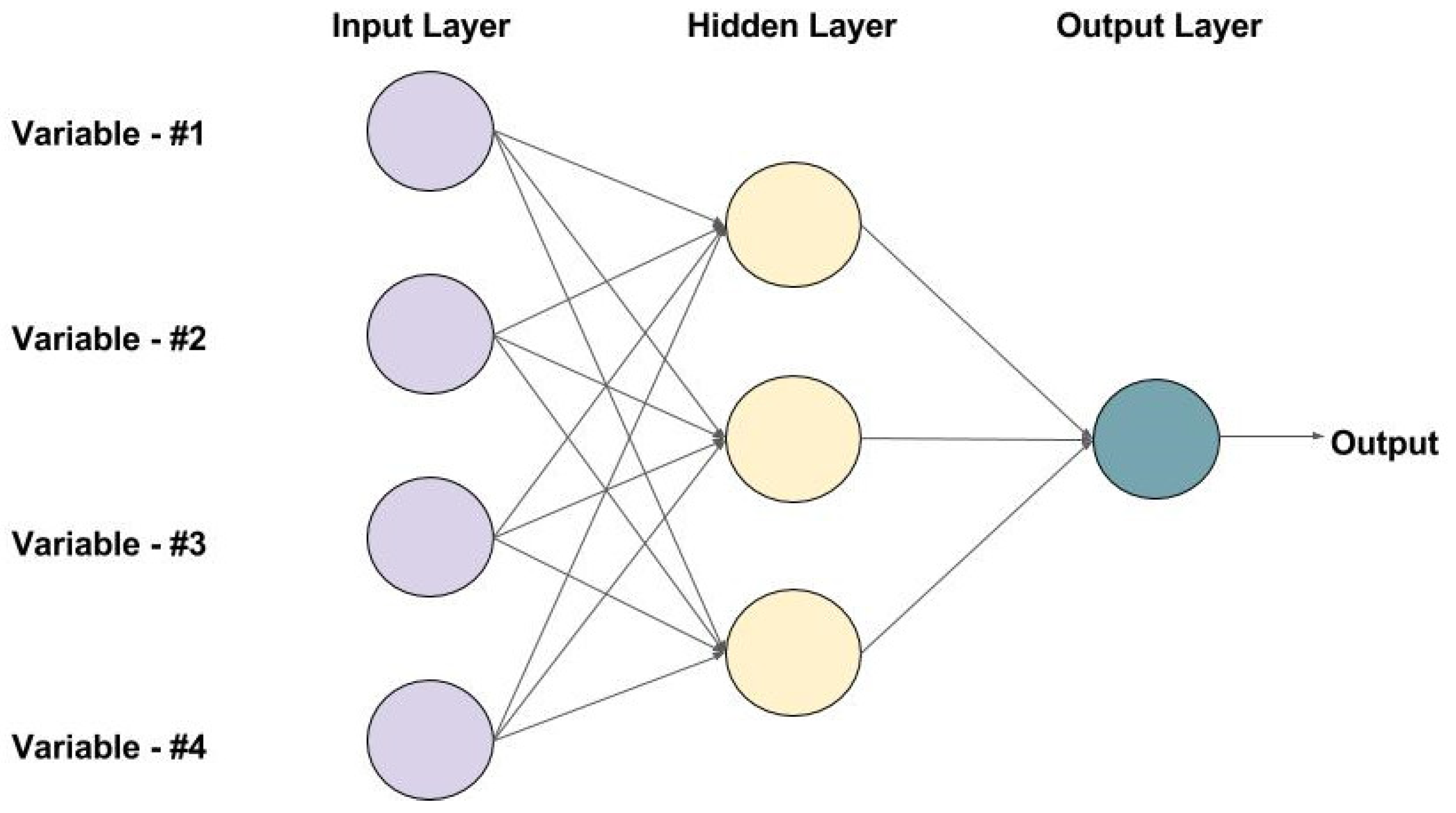
The neural network ensemble on the hand similar to the human brain in two ways: information is acquired by the network, and synaptic weights, which are the strengths of interneuron connections, are stored. In this sense, a multi-layered feedforward neural network, trained using a supervised-learning approach and operated in the MATLAB numerical computing environment was used for this study. The multi-layered feedforward neural networks consisting of three layers; the input, hidden, and output layers as shown in Figure 2. was deployed. Learning and output were calculated through backpropagation algorithms amongst the different layers, interconnected by means of synaptic weights. The input variable x = (x1, …,xn) is introduced into the neural network through the input layer. This layer is interconnected with the hidden layer h = (h1 ….,hn) through weighted edges, and subsequently, it is connected to the output layer. The weight of the edge linking the input layer to the hidden layer is represented as wkj, while wk denotes the weight connecting the hidden layer to the output layer. The output produced by the kth hidden neuron can be expressed in Equation (3) as follows:
h k = ω k 0 ( 1 ) + j = 1 p ω k j ( 1 ) x j
where:
is the activation function.
Figure 2. diagram of a multilayer feed-forward neural network.
Preprints 95596 g002
The hyperbolic tangent sigmoid function (tansig) and linear transfer function (purelin) were used for the activation function of the network while the conjugate gradient algorithm is used to change the synaptic weights and learning rate in optimization of the outputs. The search and conjugate directions are carried out simultaneously in the conjugate gradient training algorithm and it has been noted to produce fast convergence. In the conjugate gradient training algorithm, the search is performed along with conjugate directions. They generally produce faster convergence than gradient descent directions. The hyperbolic tangent function is used for the activation function and the conjugate gradient method is used as the optimization algorithm. In the multilayer perceptron of network, the minimal relative variation of the learning error is set at 0.001, and the minimum variation of the learning error was fixed at 0.0001. The calculations are repeated until the error is as small as possible. The neurons in the input layer serves as a buffer. The number of neurons in the hidden layer was adjusted to prevent overfitting, set at twice the number of independent variables, considering the optimal stimulation condition and the number of independent variables (Jang, 2017). Input selection for ANN models patterned after the method of Jang, (2021) were generated for individual study areas using the top three models (“ANN3”) or the top five models (“ANN2”) based on their ranked correlation during the historical period, as detailed in Table 2. The “ANN1” configuration, on the other hand, includes all seven of the GCMs studied.

2.4. Statistical Metrics for Model Evaluations

2.4.1. Taylor Diagram

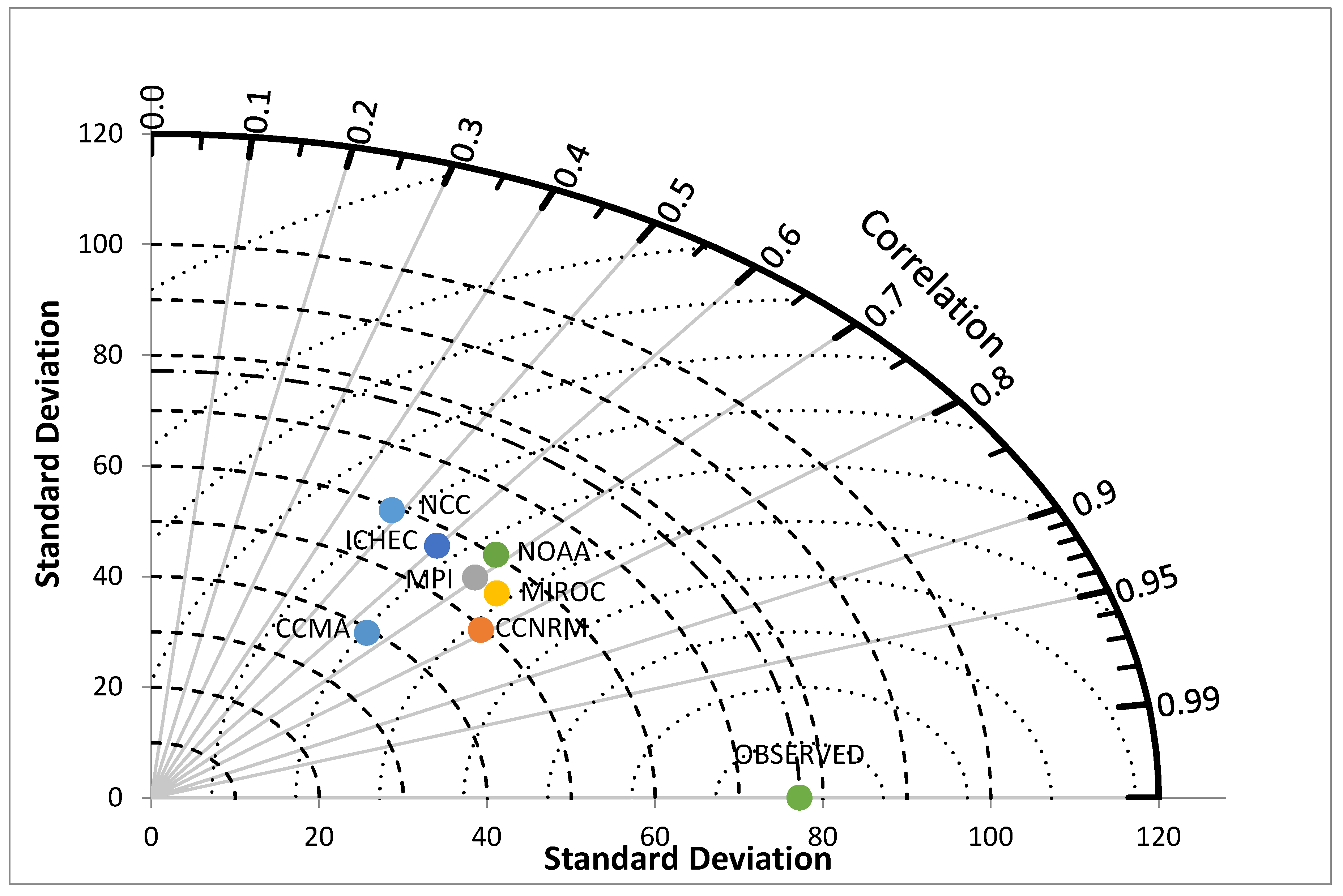
The Taylor diagram provides a graphical summary of the statistical characteristics of the climate models and the relative skill which GCMs simulate the spatial pattern of annual mean of climate variable. The Taylor diagram is used in this study to rank the performance of the seven GCMs in simulating the CRU dataset (observed). Three important metrics, the correlation coefficient (Cor.), standard deviation (σ), and centred root mean square error (cRMSE) are displayed on the diagram (Taylor, 2005). The centred root-mean-square is difference between the GCMs and the CRU and represented as the radial distance to the point on the x-axis identified as “observed.” Also, the σ measures the average dispersion of the outputs of the datasets away from its mean, represented on the Taylor diagram as the distance from the origin. Finally, the Correlation coefficient measures the strength and direction of the linear association between the GCMs and the observed. The description of the correlation is then made using the delineation by (Handoko et al., 2019) as displayed on Table 3. Equations (3)–(6) below, displays the formula for the estimation of the correlation coefficient, the centred root men square error and the standard deviation between two Models a and b as displayed on the Taylor diagram.
C o r . = 1 n i = 1 n ( a a ¯   ) ( b b ¯   ) σ a σ b
σ a = 1 n i = 1 n ( a a ¯   ) 2
σ b = 1 n i = 1 n ( b b ¯   ) 2
c R M S E = 1 n i = 1 n ( b b ¯   ) 2 ( a a ¯   ) 2
where:
σa and σb are the standard deviations of Model “A” and Model “B” respectively
Table 3. ANN Ensemble Design.
S/N Station Name Case Variable ANN Ensemble Inputs
1 Ilorin ANN 3 Precipitation CNRM-CM5, MPI-ESM-LR, GFDL-ESM2M
ANN 2 CNRM-CM5, MPI-ESM-LR, GFDL-ESM2M , EC-EARTH, MIROC5
ANN 3 Tmax CNRM-CM5, CanESM2, MPI-ESM-LR
ANN 2 CNRM-CM5, CanESM2, MPI-ESM-LR, MIROC5, NorESM1-M
ANN 3 Tmin CanESM2, NorESM1-M, GFDL-ESM2M
ANN 2 CanESM2, NorESM1-M, GFDL-ESM2M, EC-EARTH, MPI-ESM-LR
ANN 1 Precipitation/ Tmax/Tmin CanESM2, CNRM-CM5, EC-EARTH, MIROC5, MPI-ESM-LR, NorESM1-M, GFDL-ESM2M

2.4.2. Mean Absolute Error (MAE), Root Mean Squared Error (RMSE) and Nash–Sutcliffe Efficiency (NSE)

The mean absolute error (MAE), root mean square error (RMSE), and Nash-Sutcliffe efficiency (NSE) were used to evaluate the accuracy of the ANN ensembles developed. The RMSE compared to the MAE is designed to penalise large prediction errors in the dataset as each error influences the overall error in proportion to its square rather than its direct magnitude. The accuracy assessment of the ensembles is done by comparing the values generated from the ensemble networks and the observed in the validation dataset. When MAE and RMSE are smaller, the estimated value indicates higher accuracy and shows how big of an error we can expect from the forecast on average.
The Nash-Sutcliffe model efficiency coefficient (NSE) is commonly used to assess the predictive power of hydrological discharge models. Nash-Sutcliffe efficiency ranges from negative infinity to 1 with an efficiency of 1 indicating a perfect match between the ensembles. whereas an efficiency less than 0.0 occurs when the observed mean is a better predictor than the model.
M A E = i = 1 n y i x i n
R M S E = i = 1 n ( y i x i ) 2 n
N S E = 1 i = 1 n ( y i x i ) 2 i = 1 n ( y i y ¯ ) 2
where:
yi=prediction
xi=true value
n=total number of data points

2.5. Mann-Kendall Trend Test

The Mann–Kendall (MK) test, which is often used to test trends in hydro-climatological time series. MK trend test is applicable in cases when the data values (x) of a time series obeys Equation (10).
χ = f t + t  
where f(t) is a continuous monotonic increasing or decreasing function of time and the Residual t can be assumed to be from the same distribution with zero mean. The MK test was executed in the R-Studio environment. The MK test statistic S is as given by Equation (11). (Salami et al., 2014):
S = k = 1 n 1 j = k + 1 n s i g n ( x j x k )
where n is the length of the time series xi…. xn, and sgn(·) is a sign function, xj and xk are values in years j and k, respectively. The expected value of S equals zero (E[S] = 0) for series without trend and the variance is computed as given in Equation (12):
σ 2 S =   1 18 n n 1 2 n + 5   p = 1 q t p ( t p 1 ) ( 2 t p + 5 )  
where q is the number of tied groups and tp is the number of data values in pth group. The test statistic Z is as defined in Equation (13):
Z =   s 1 σ 2 ( s )   i f   S > 0 0   i f   S = 0 s + 1 σ 2 ( s )   i f   S < 0  
As a non-parametric test, no assumptions as to the underlying distribution of the data are necessary. The Z-statistic is then used to test the null hypothesis, Ho that the data is randomly ordered in time, against the alternative hypothesis, H1 where there is an increasing or decreasing monotonic trend. To estimate the true slope of an existing trend, the Sen’s non-parametric method was used.3. Results
This section may be divided by subheadings. It should provide a concise and precise description of the experimental results, their interpretation, as well as the experimental conclusions that can be drawn.

3. Results

The results are presented and analyzed across various segments, each shedding light on distinct aspects of the climatic and meteorological conditions in Nigeria. Section 3.1, delves into the historical metrological information through the examination of observational datasets and provides a nuanced understanding of temperature and rainfall patterns within specific regions. Moving forward to Section 3.2, the focus shifts to a meticulous comparison between observed data and GCMs, employing Taylor diagrams to assess the statistical performance of various models in simulating precipitation, maximum temperature, and minimum temperature. Section 3.3 introduces a comparison between ANN, MLR and AM Ensembles, identifying the most accurate and robust modeling approach for forecasting climatic variables. The subsequent Section 3.4 delves into the accuracy assessment of ANN ensembles, utilizing multiple error metrics for a comprehensive evaluation. Following this, Section 3.5 conducts a trend analysis of historical rainfall and temperature, offering insights into climate variability over time, specifically focusing on representative stations in different agroecological zones. Finally, Section 3.6 explores the spatial representation of changes in mean temperature and annual rainfall, providing a comprehensive assessment of the observed trends and projecting future scenarios under different climate change pathways.

3.1. Summary of Historical Metrological Information (Observation Dataset)

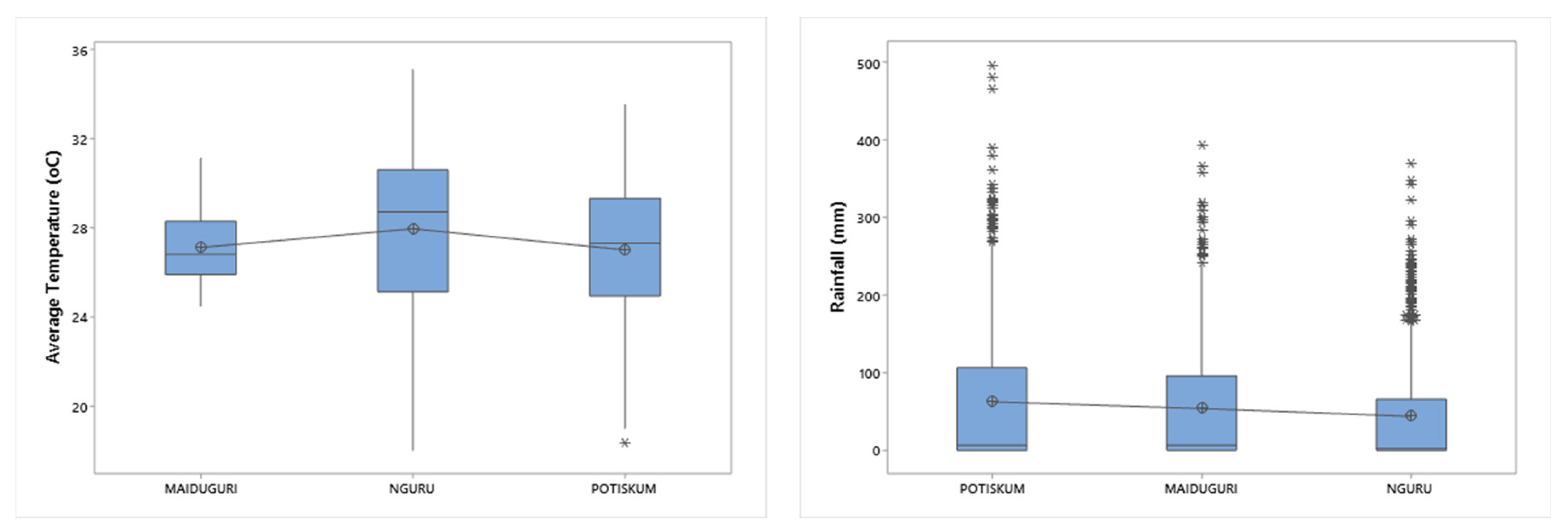
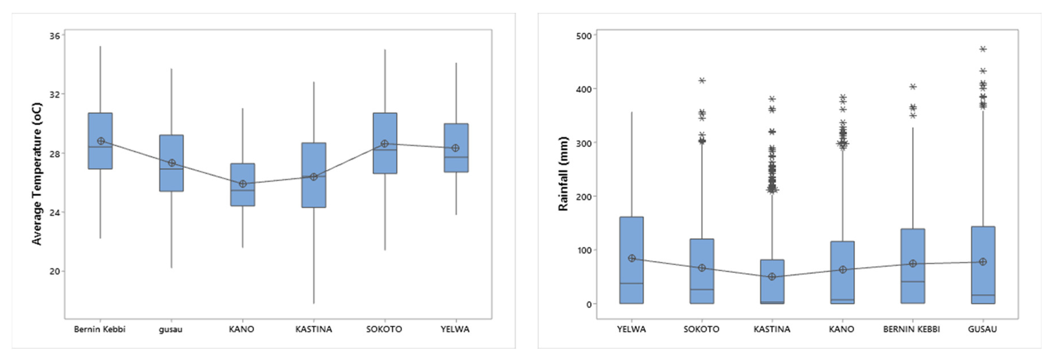
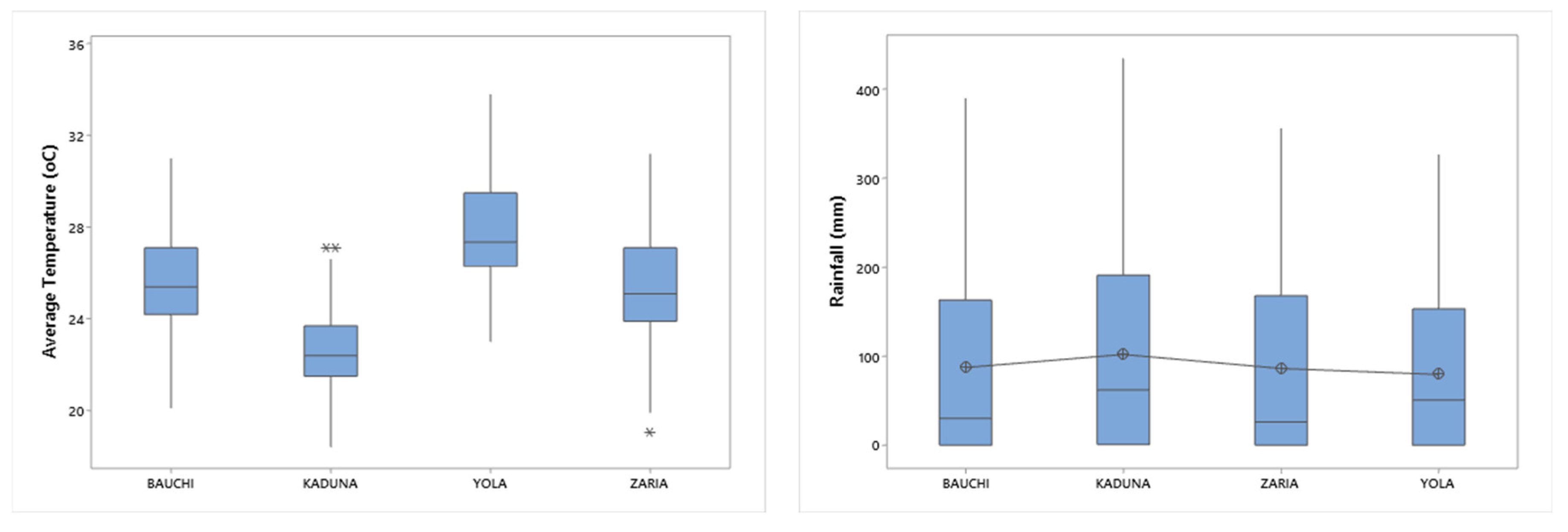
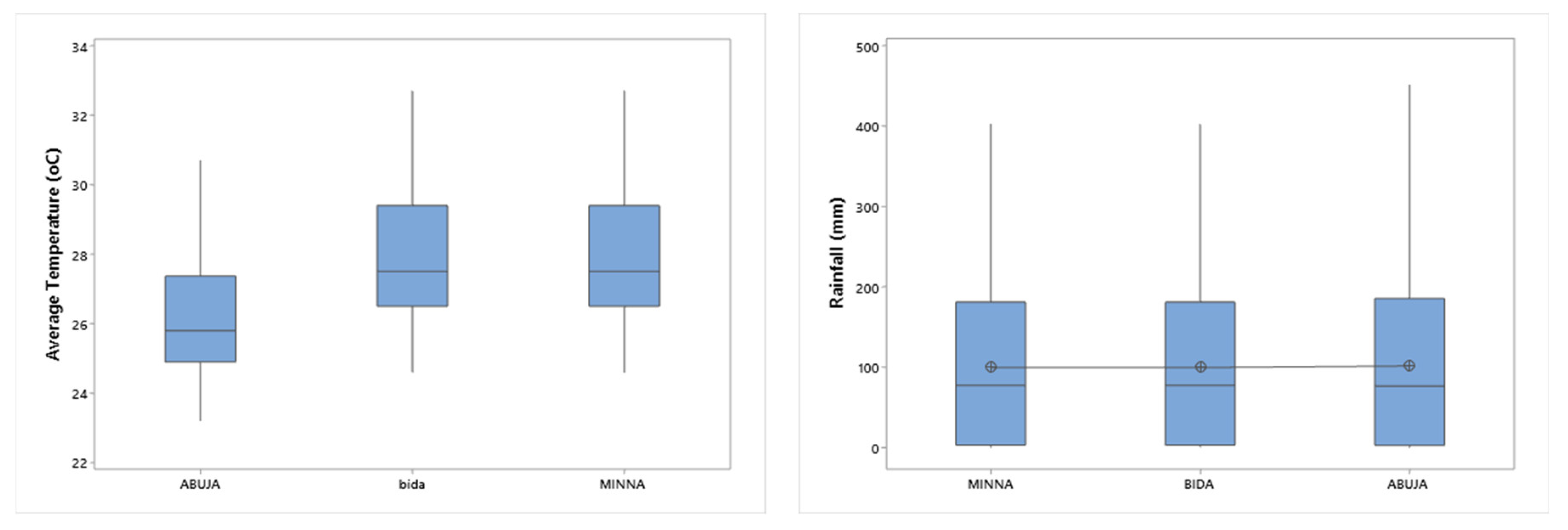
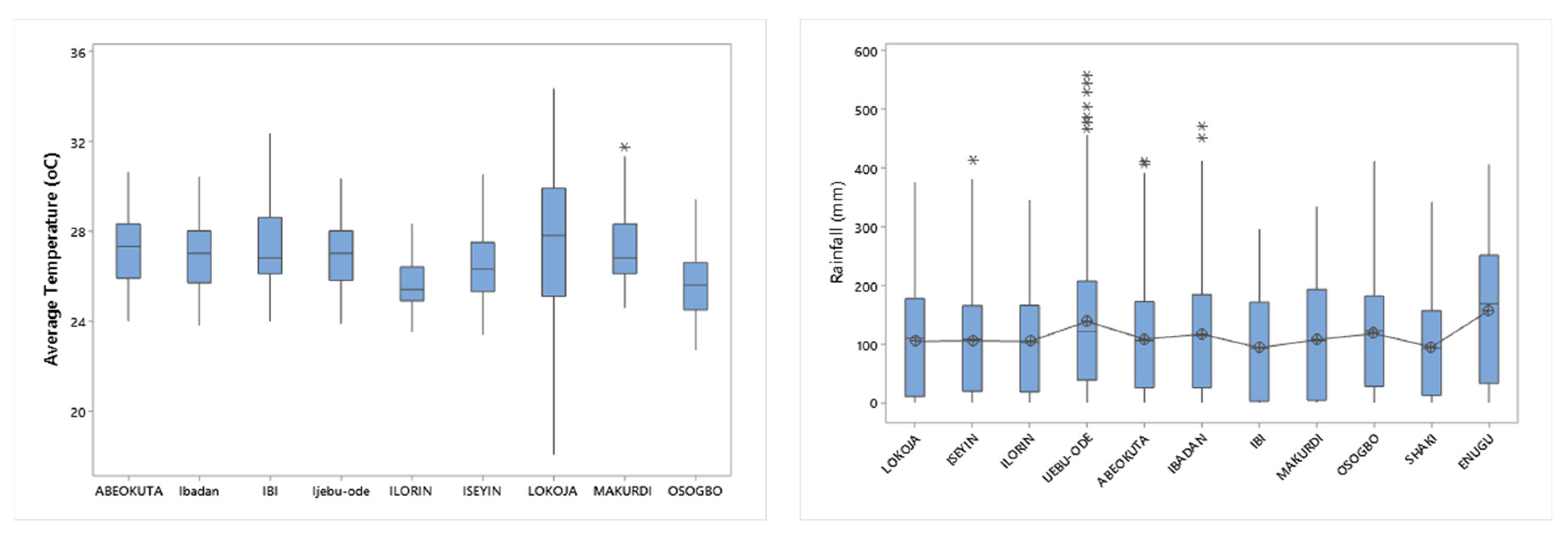
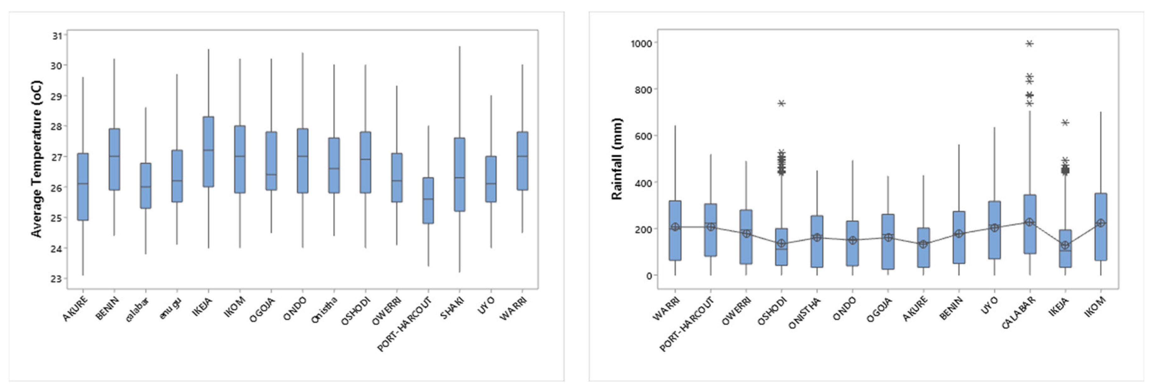
The observational dataset (CRU) and GCMs were extracted to forty-one (41) WMO/NiMET locations across the study area for easy reference. The GIS locations and elevation of each observation station are provided in the Supplementary Materials. The observational dataset is used for the validation of the statistically downscaled GCM ensembles. The dataset is then grouped into seven clusters, Sahel Savannah (SAS), the Sudan Savannah (SUS), the Northern Guinea Savannah (NGS), the Southern Guinea Savannah (SGS), the Derived/Coastal Savanna (DRS), the Mid-Altitude (ALT) and the Humid Forest (HMF) agroecological zone patterned after (Mereu et al., 2015). The box and whisker plots are employed as a descriptive statistical tool in identification of outliers and assessment of normality of the dataset (Figure 3, Figure 4, Figure 5, Figure 6, Figure 7 and Figure 8).
The Potiskum, Maiduguri and Nguru stations are situated in the SAS zone with an interquartile range (IQR) for temperature ranging from 25-29.6°C, 26.1-28.4°C and 25.5-30.75°C. Statistically the chance that future temperature will fall to this range is 50%. Lange & Vinke, (2021) reports that Africa’s Sahel has a tropical semi-arid climate, typically hot, sunny, and dry in accordance to Koppen climate classification. The small length of IQR in comparison to the whiskers also suggest a middle clustering of the data about the median values of 27.4°C, 28.8°C and 26.9°C. Also, the Maiduguri observational station presents a more reliable dataset in deterministic modelling due to the relative smaller dispersion of its value. The rainfall values in the region are significantly skewed with mean values of 62.76, 43.91 and 54.01mm/month in comparison with low median values of 6.75, 2.7 and 6.9mm/month. Generally, positive skewness suggests a positive deviation from the median and the outlying values are less probable in that direction. Ordinarily, this may imply increase in rainfall values for the region but the employed descriptive tool doesn’t factor in the non-parametric temporal attributes of the dataset. At the SUS zone, the Katsina station dataset has the smallest dispersion for rainfall, between 81.5-0.73mm/month. The large presence of outliers in most of the station in this zone is indicative of the changing pattern of the dataset in the region. Several reports have highlighted the changing pattern of climate in the Sudan agroecological zone (Mertz et al., 2012; Siddig, Stepanyan, Wiebelt, Grethe, & Zhu, 2020). Also. the rainfall values in the region are significantly skewed with low median values of in comparison with higher mean values of for the SAS zone. The IQR of temperature values in the region are 30.1-26.8°C, 30.7-26.8°C, 28.9-24.4°C, 27.5-24.5°C, 30.9-27°C, and 29.3-25.5°C with slight negative skewness is also observable in the temperature pattern at the Yelwa, Sokoto, Kano, Birnin-Kebbi and Gusau station respectively.
At the NGS zone, IQR shows a compact dataset for the region. For the observational stations in Zaria, Yola, Kaduna, and Bauchi, it runs from 27.4-24°C to 29.7-26.4°C to 21.52-24°C to 27.4-24.3°C, respectively. The rainfall values in the region are also skewed similar to the datasets in the SUS, but with a closer median to mean values and higher rainfall values. The median values of 26.25, 50.65, 62.15, 20.15mm/month to mean values of 86.22 and IQR length ranging from 168-0.2, 153.38-0, 191.4-0.6, 161.15-0.2mm/month are recorded for the Zaria Yola, Kaduna and Bauchi stations respectively. The Kaduna station recorded higher rainfall values (mean of 62.15mm/month) and it’s known as a commercial hub in the geopolitical region. Blanc & Perez, (2008) work on the correlation between rainfall and human density largely explains the relative increased commercial and agricultural activity in this basin, however, larger population leads to increased production of GHG and water stress. From literature the SGS is reported to have more rainfall and denser vegetation in comparison with the NGS (Adenle, et al., 2020; Ayanlade, 2009). A broad comparison between the box and whisker plots of the NS and SGS zones, demonstrably explains this difference. The temperature of the region is higher in the SGS compared to the NGS but the rainfall values are also higher in the SGS. This may be as a result of the relative incidence of the sun to the two regions. Because the equator is located in the direct plane of the sun, the SGS closer to the equator receives relatively more solar radiation in comparison the NGS. The mean values of rainfall in the two regions are similar but with a more asymmetrical dataset for the SGS, which in meteorological terms, may imply longer rainy season. The temperature presented in the DRS zone is milder in comparison to the other guinea savannas. At the Ilorin station temperature dataset presents an almost ideal dataset with little dispersion and skewness with the relative short tails of the whiskers to the box plot indicative of a bimodal distribution of temperature values. The IQR ranges from 25-26.6°C, a mean of 25.7°C, and a median of 25.5°C. Temperature ranges between 25-35°C has been reported to be optimum for several crops grown in the tropics (Adedapo, 2020; Akpenpuun & Busari, 2018; Ghadirnezhad & Fallah, 2014). The mean DRS rainfall values are also slightly higher than the SGS rainfall values (except for the Shaki and Ibi stations). The Ilorin rainfall also datasets presented a fairly symmetric dataset with IQR range between 145.575-19.25mm/month. At the HMF zone rainfall datasets in the region are slightly skewed with the median values generally higher than the mean values for many of the stations. The observable long tails of the whiskers and the outliers also indicates a changing pattern of rainfall in the region. The temperature datasets assumed a fairly symmetrical nature with a diverse IQR range amongst the stations, with the Port-Harcourt, Akure and Calabar stations returning much lower IQR range compared to others, the observation stations seem to belong to different climatological zonation. Contrariwise, this study considers agroecological zonation, which according to the FAO not only considers climate but landform, soils, land cover and its potentials for agriculture (Mereu, et al. 2015)

3.2. Comparison between Observed (CRU) and GCM Dataset

Taylor diagrams ranking the statistical performance of the GCMs for precipitation, maximum temperature and minimum temperature at each location during the observation period (1950-1994) are displayed in the Supplementary Material. These diagrams reveal variations in the statistical characteristics’ similarity among GCMs, depending on the specific variable and location. Figure 9 below illustrates a typification of the performance ranking of GCMs for rainfall in the SAS using the Taylor diagram.
The CNRM-CM5 model demonstrated the highest correlation and consistently provided the most accurate simulation of observed rainfall across all stations, with a mean absolute error falling within the range of 52-70mm per month. Gnitou et al., (2019) also reports that the CNRM-CM5 ranks among the best performing models in the simulation of rainfall in west-Africa. Nevertheless, when assessing the CNRM-CM5 model’s capacity to reproduce the magnitude of rainfall datasets, the results were less encouraging. For instance, at the SAS representative city, the GFDL-ESM2M outputs exhibited a standard deviation closer to the observed data. The standard deviations of the GCMs for rainfall at the station all indicated a lower amplitude compared to the observed data, suggesting that the GCM values tend to cluster more closely around their mean than the observed data.
The correlations of the outputs of Tmax GCM models displayed a weaker correlation in the Sahelian regions compared to the humid regions of the country. For example, the outputs of Tmax at the SUS returned a low to a moderate correlation compared with the high correlation of all the GCMs at the HMF. Also, the MIROC5, NorESM1-M and MPI-ESM-LR temperature models all rank highly by the cRMSE metric but with low ranks for emulating the standard deviation. Notably, the GFDL-ESM2M model, though with a comparatively weaker correlation amongst the tmax models best mimicked the temporal variability of maximum temperature across the zones with the exception of the HRF and SAS.
Overall, the Tmin displayed weak correlations, with models such as CanESM2 and EC-EARTH, performing relatively well especially in the Sahelian and Sudan regions. CNRM-CM5 model which erstwhile ranked highly for rainfall simulation and Tmax ranked poorly in the simulation of Tmin. It is noteworthy that GCMs with low correlation values in some cases prove to be the best in simulating data amplitudes, emphasizing the importance of a Multi-Model Ensemble approach in meteorological forecasting across different variables and stations.
Hence, the selection or rejection of a GCMs based on strength of correlation as employed in the works of Handoko, et. al., (2019) is a hasty generalization as a GCM may not have strong performance in certain aspect but possess strength in others. Similarly, Rowell et al. (2016) study which focused on distinguishing CMIP5 GCMs in the context of Africa, reveal divergence in GCM performance based on different metrics. Notably, even when selecting more capable models based on an overall performance measure, projection uncertainty persists since these models tend to span the entire spectrum of projections.
Demonstrable in Tmin simulation by the MIROC5 in the DGS and HMF; Tmax simulation by the GFDL-ESM2M in the DGS and NGS and the NorESM1-M at the ALT and NGS. In addition, it presents more evidence that bias correction methods based on fixed additive methods or linear relationship between GCMs and observed as employed by the methods of Nurul, (2018) and Alioune, (2021) are unreliable in the region. Also, linear bias correction may be sometimes unsuitable due to the GCMs limitations in capturing local nuances, requiring more advanced techniques for reliable results

3.3. Comparison between ANN, MLR and AM Ensembles

Multiple regression displayed on equations 14 to 20 are used to forecast precipitation; then these results were compared with ANN’s forecast. Equations for Tmax and Tmin are given in the Supplementary Materials section.
RainSAS = 7.847 + 0.091CanESM2 + 0.391CNRM-CM5 - 0.091EC-EARTH + 0.370MIROC5 + 0.178MPI-ESM-LR + 0.145NorESM1-M - 0.152GFDL-ESM2M
RainSUS = 9.173 - 0.057CanESM2 + 0.610CNRM-CM5 + 0.068EC-EARTH + 0.192MIROC5 + 0.243MPI-ESM-LR - 0.176NorESM1-M+ 0.166GFDL-ESM2M
RainNGS = 5.661 - 0.055CanESM2 + 0.549 CNRM-CM5 + 0.026EC-EARTH + 0.244MIROC5 + 0.162MPI-ESM-LR - 0.218NorESM1-M + 0.278GFDL-ESM2M
RainDGS = 15.659 - 0.126CanESM2 + 0.187CNRM-CM5 + 0.051EC-EARTH + 0.249MIROC5 + 0.260MPI-ESM-LR - 0.190NorESM1-M + 0.225GFDL-ESM2M
RainSGS = 6.026 - 0.043CanESM2 + 0.352CNRM-CM5 - 0.087EC-EARTH + 0.206MIROC5 + 0.183MPI-ESM-LR - 0.045NorESM1-M + 0.222GFDL-ESM2M
RainALT = 4.208 + 0.007CanESM2 + 0.192CNRM-CM5 - 0.024EC-EARTH + 0.113MIROC5 + 0.109MPI-ESM-LR + 0.227NorESM1-M + 0.047GFDL-ESM2M
RainHMF = 14.387 - 0.053CanESM2 + 0.231CNRM-CM5 + 0.025EC-EARTH + 0.142MIROC5 + 0.207MPI-ESM-LR + 0.003NorESM1-M + 0.174GFDL-ESM2M
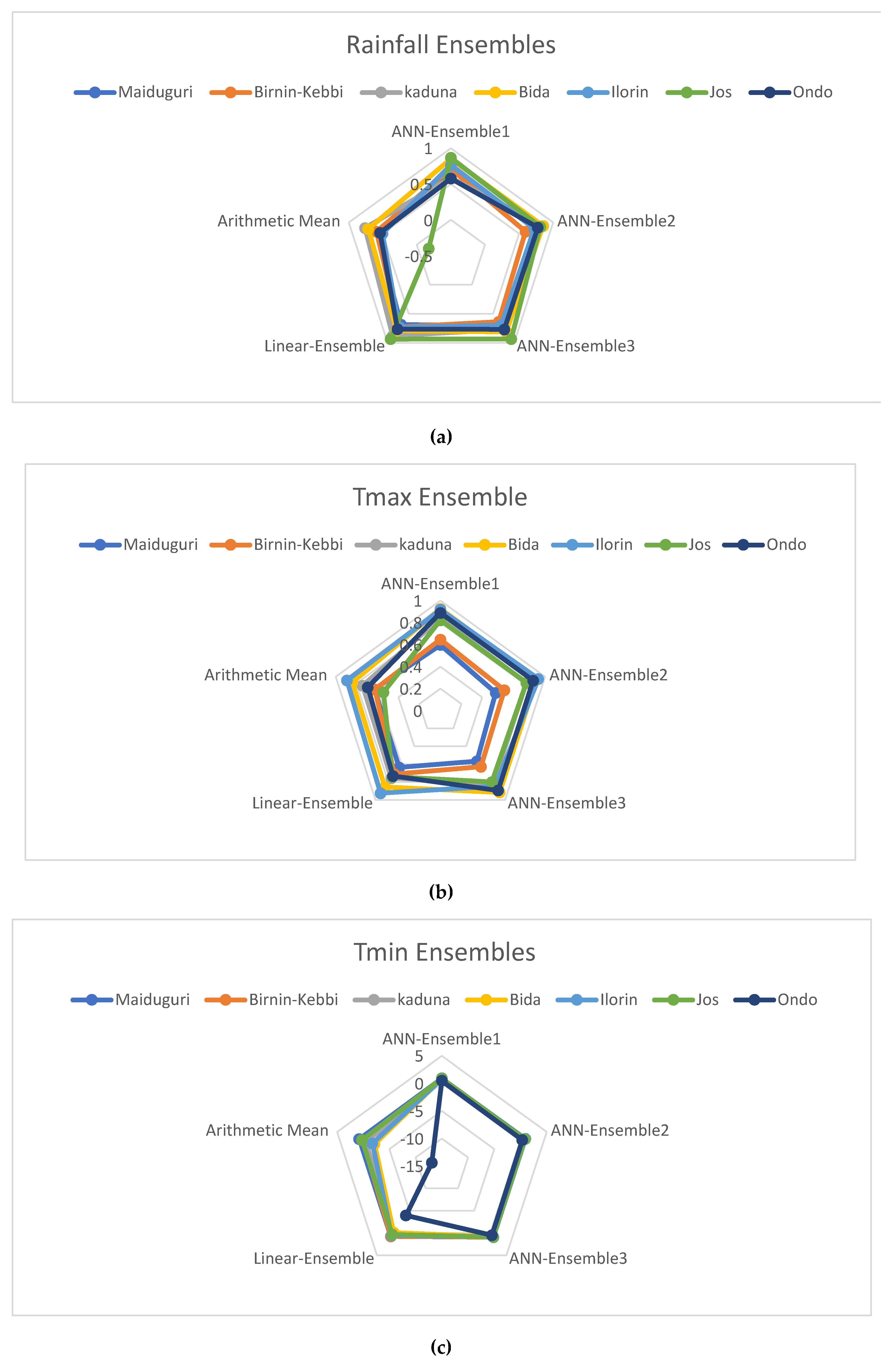
To provide a comprehensive comparison of ensemble models, Figure 13 summarizes the results based on NSE, which is considered the most suitable error metric for this study (other metrics are provided in Supplementary Table S7). NSE is uniquely designed for hydrologic modelling and effectively conveys the predictive capabilities of the models in this context.
While, the ANN ensemble outperformed all singular GCMs in the modelling of climate variables, the MLR ensembles did not yield noticeable improvements in predictive performance at certain meteorological stations, particularly when focusing on minimum temperature. An illustrative example of this phenomenon can be observed at the Ondo station. Here, the low-performing models within the rainfall ensemble, selected based on their correlation patterns, exhibited some degree of predictive skill, albeit limited in scope. Consequently, the inclusion of these models may be adjured to have contributed to an enhancement in the overall predictive capability. However, in contrast, within the temperature MLR ensemble, a different scenario emerged. These GCMs, introduced substantial errors into the ensemble’s predictions, resulting in a noticeable degradation of the ensemble’s overall performance. This disparity in the impact of low-performing models underscores the complexity of model ensembles and the efficacy of ANN in decoding such complexities in different meteorological context.
Higher correlation between Rainfall Climate Models (GCMs) and observed climate data during the observation period does not necessarily result in significant improvements in ensemble outputs, unlike the notable enhancements seen in temperature models. Tolle, et al., (2019) pointed out that Rainfall GCMs might exhibit stronger correlations because they capture broader precipitation patterns, including the timing and distribution of rainy seasons and dry spells. However, these models face challenges in representing local-scale variations influenced by factors like topography, land use, and convective processes. Correcting these local-scale biases can be more intricate compared to temperature biases, which often stem from broader atmospheric dynamics. As a result, improving the performance of rainfall GCMs may necessitate more sophisticated techniques, aligning with Crawford et al.’s (2020) assertion that predicting precipitation is notably more complex than predicting temperature.

3.4. ANN Ensemble Accuracy Assessment
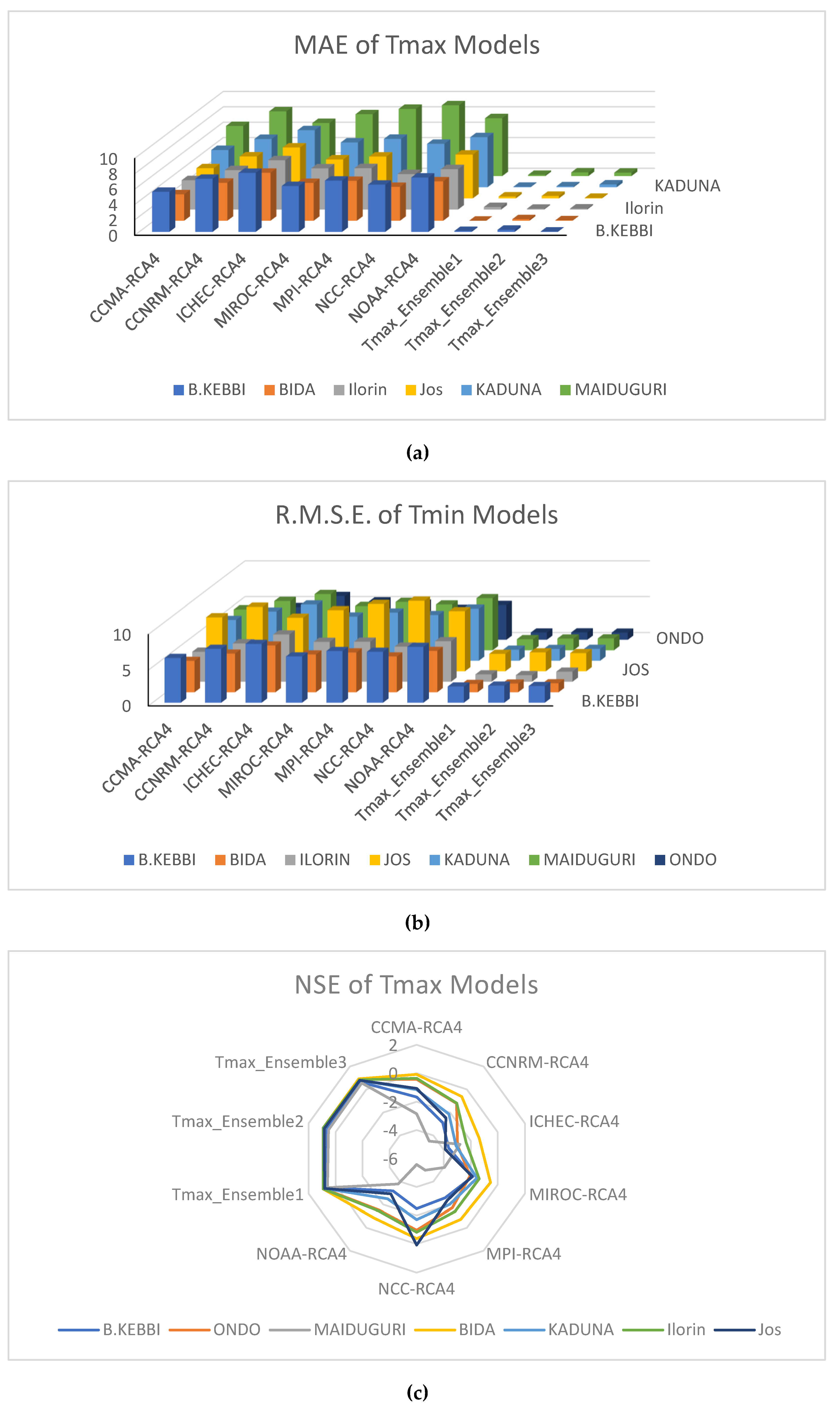
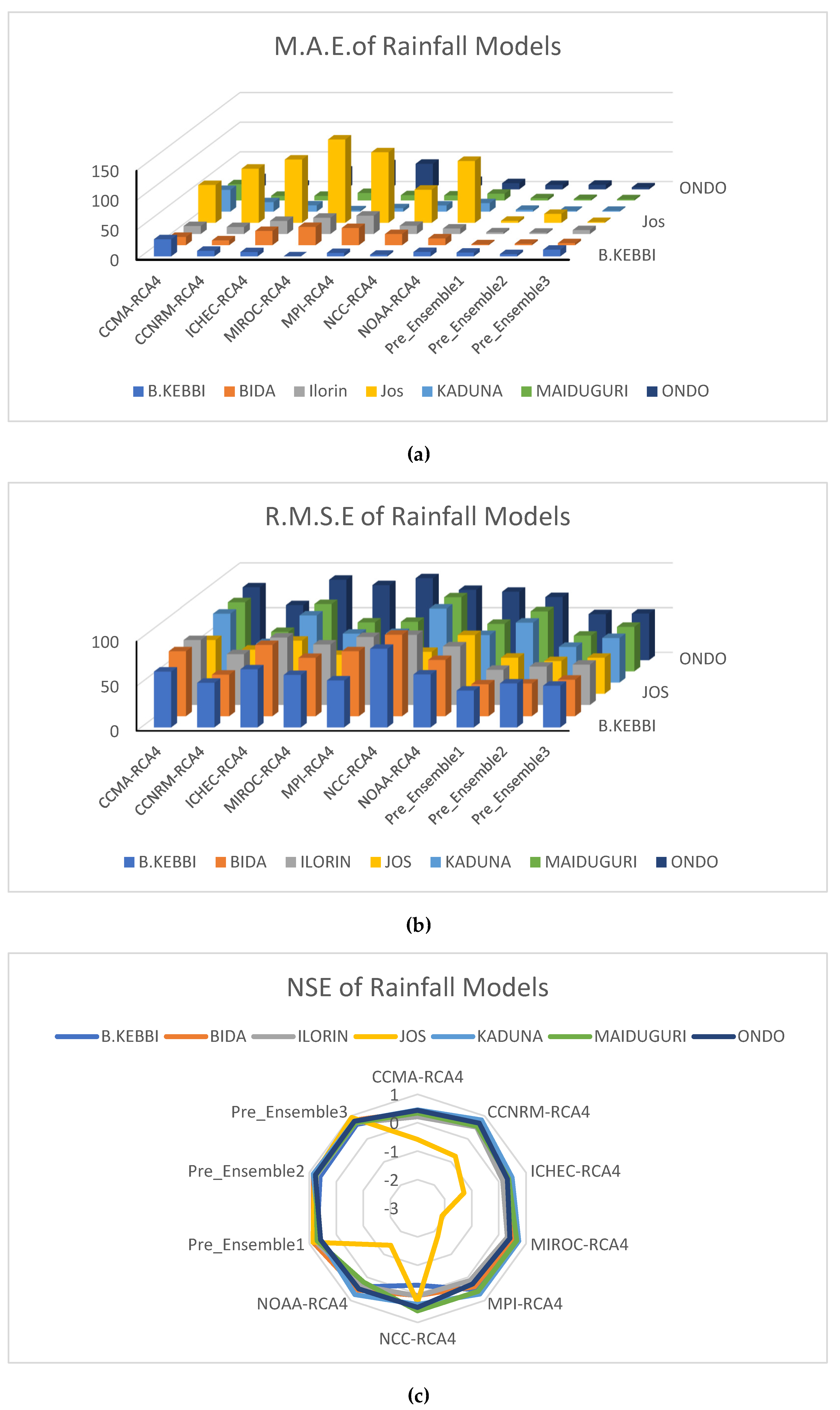
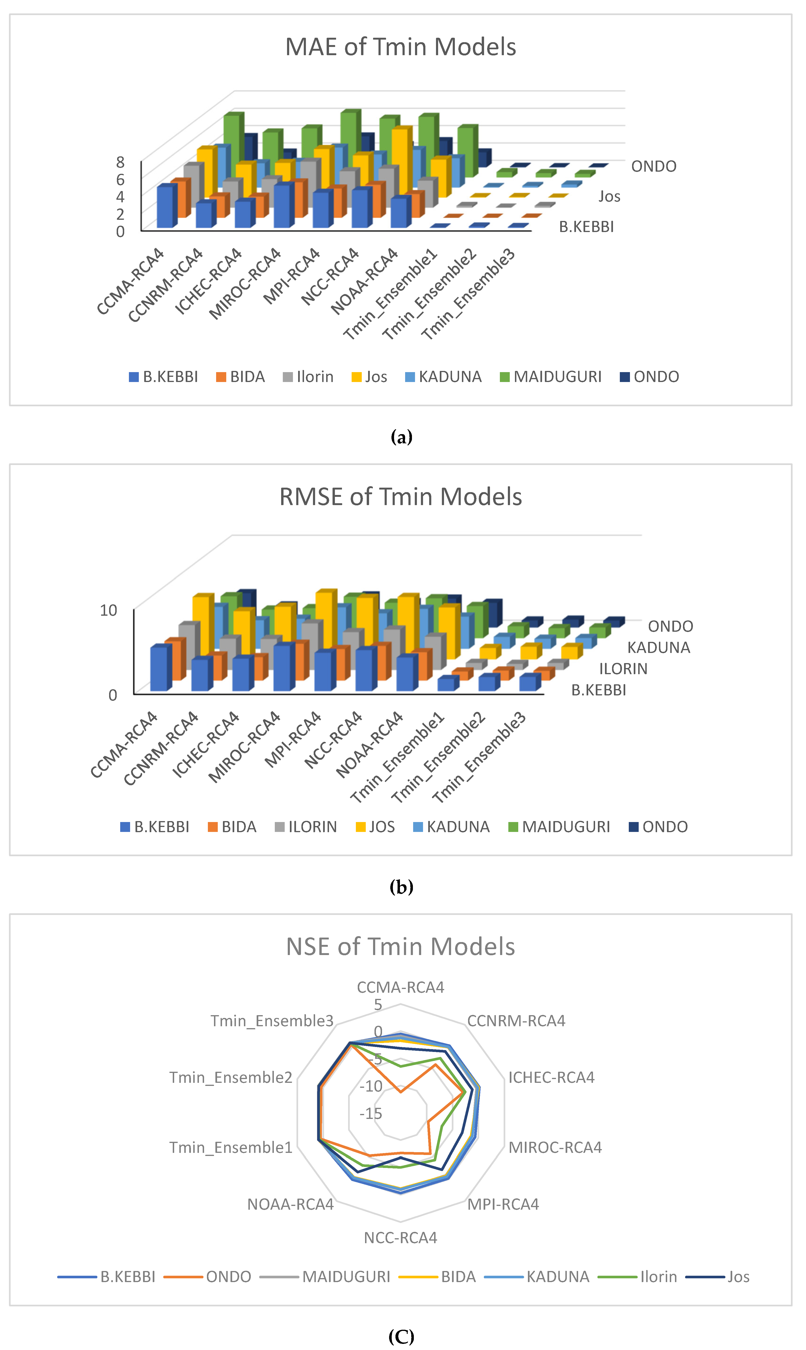
The accuracy of the ANN ensembles developed for each variable in each of the analysis station were assessed. Performance of the ensemble methods were compared for an evaluation period; 1995-2005. Three error metrics are used to assess the performance of the ensembles, the MAE, RMSE and NSE metrics. This metrics were selected to project the multidimensional nature of assessing climate and hydrological modelling. It has been established that the use of a single error metric in model performance evaluation will only highlight a limited aspect of the error characteristic (Willmott & Matsuura, 2005). Accuracy assessment of GCMs/ensembles varied across the analysis stations based on the error metric and are presented in Figure 10, Figure 11 and Figure 12.
Figure 10. Rainfall GCMs/ ANN Ensembles accuracy assessment using: (a) MAE, (b) MSE, (c) NSE.
Preprints 95596 g010
Figure 11. Tmax GCMs/ ANN Ensembles accuracy assessment using: (a) MAE, (b) MSE, (c) NSE.
Preprints 95596 g011
Figure 12. Tmin GCMs/ ANN Ensembles accuracy assessment using: (a) MAE, (b) MSE, (c) NSE.
Preprints 95596 g012
Figure 13. Comparison of Ensemble methods for (a) Rainfall (b)Tmax, (c) Tmin.
Preprints 95596 g013
To assess ensemble agreement with observations quantitatively, accuracy evaluation was structured to address general statistical aspects of model performance that do not pertain to any specific application. Similarly, in order to present evaluation results in line with the natural temporal resolution of the observational datasets, without any aggregation or alteration, we limited our analysis to the monthly scale. The graphical representation of the best performing ANN ensemble in each station against the least accurate GCM are displayed in the Supplementary Materials section. An illustration of climate model enhancement for a specific application is evident in the comparison of monthly precipitation between less accurate GCMs and an optimized ensemble for the ALT, as presented in the Supplementary Figures. The temporal trend of the outputs provides strong evidence of reduced overestimation of rainfall during the rain seasons by GCMs. This “wet bias”, noted by Gnituo et al. (2019), brought about by the exaggerated depiction of the West African Monsoon convergence zone, especially from June to September were corrected (see Supplementary Figure S4).
The ANN ensembles developed all outperformed the individual GCMs outputs for all stations vis-à-vis the three-error metrics with varying differences, except for rainfall at Birnin-Kebbi station. Selecting the ideal model requires discrete consideration based on the intension for use. By way of illustration, accuracy assessment of precipitation models using MAE at the Birnin-Kebbi station ranked the MIROC5 model highest. However, it is important to note that the proportional scale of the error is not always clear with the MAE, a major disadvantage of the metric (Willmott and Matsuura, 2005). Demonstrably, the RMSE which best shows the impacts of large errors in the forecast ranks the MIROC5 fourth while the NSE ranks it sixth. Therefore, the ANN1 ensemble which is jointly ranked best by NSE and RMSE may be more suitable if considerations of weather extremities will be executed.
The performance of ensembles varied across different factors, including the specific methods used, variables examined, the choice of error metrics, and geographical locations. In general, ensembles significantly improved predictive performance, particularly as measured by the NSE. These improvements were notable, with a 34% enhancement for rainfall, a substantial 255% improvement for maximum temperature (tmax), and an impressive 660% boost for minimum temperature (tmin). Furthermore, the ensembles contributed to a reduction in errors, as assessed by the RMSE. This reduction was quantified at 26.51% for rainfall, 77.09% for tmax, and 64.58% for tmin (refer to the Supplementary Table S6 for details). The performance differences between ensembles for rainfall and temperature were primarily linked to variations in the complexity and complementarity of the individual models associated with each variable.
For instance, when simulating rainfall, it was observed that the ensemble accuracy was higher when excluding the NorESM1-M and GFDL-ESM2M models from the ensemble design. Moreover, in specific locations like the Maiduguri station (SAS), the ANN3 ensemble, which included the CNRM-CM5, MIROC5, and MPI-ESM-LR models, displayed a notably low average absolute error of 2.17mm per month, a substantial improvement compared to the large error margin of 27.47mm per month observed in the individual CanESM2 model. Conversely, the RMSE and NSE metrics ranked the ANN2 ensemble as the best performer in simulating precipitation at the station. Similarly, at the ALT observation station, individual GCMs exhibited substantial errors, with the MIROC5 model showing an average error of 140mm per month during the evaluation period. These deficiencies were markedly rectified using the MME approach, which reduced the error to a minimal 1.4mm per month for the ANN3 ensemble, accompanied by a notably high predictive power of 93%.

3.5. Trends Analysis of Historical Rainfall and Temperature

The overview of the historical dataset in section 3.1 evidently shows a changing pattern for climate with temperature on the increase and observable presence of outliers in rainfall data. In a bid to situate the presence and quality of trend at each of the agroecological zone several time-series trend analyses were conducted. The selected representative stations in each of the seven agroecological zones were analysed. The monthly trend test for average temperature and precipitation for the time series data for all the locations are presented in Table 4. Positive z-values show an upward tendency, whilst negative values show a downward trend.
At the Maiduguri observation station, with the exception of January, which saw a slight decline and a negative z-value of 0.8, the trend of mean temperature is significantly on the rise. The Sen’s slope estimator, which measures the strength of the trend in the time series, also reveals that April is the month most negatively impacted. Ogunrinde et al., (2020) projected that rising temperature in the Sahel may lead to increase incidences and intensity of drought. The UN climate risk assessment profile has also noted that the Sahel region is one of the most vulnerable to CC with the warming climate to lead to higher reduction in agricultural output in the region in comparison to the reductions of global outputs; a consequence of this will be to further put food security at risk. (Sallaba et al., 2017). Rainfall is not widely varied from the MK trend test. With little or no amount of rainfall recorded in five months, five out of the remaining months returned an upward trend while the months of May and August had decreasing trend though not significant. The Sahel has been reported to be experiencing an increase in summertime rainfall (Bichet & Diedhiou, 2018; Kumi et al., 2021; Pausata et al., 2020). The regional monsoon circulation and the global Hadley cell are both dynamically connected to the Sahel’s rainfall. As a result, it is vulnerable to regional land effects like rising temperatures and changes in greenhouse gases brought on by anthropogenic activities as well as local forcings from distant waters. These mechanisms can account for the apparent interannual fluctuations in the region.
The densely populated Sudan Savannah agroecological zone returned a positive z-value of 6.9 for the yearly average mean temperature and a Sen’s slope value of 0.024 for the month of April (the largest change), the trend analysis shows that the temperature in the area is significantly rising. From a yearly average temperature of 26°C in the 1950s to approximately 28°C in the 2010s, the temperature has steadily increased. The record high monthly average of 30.40°C for the month of February in the year 2010 eloquently demonstrates this. Rainfed agriculture, aquaculture, natural ecology systems and biodiversity, water resources, and energy are the sectors of the Sudan agroecological zone that are most susceptible to temperature increases, according to Siddig et al., (2020). While August typically received the biggest quantity of rainfall over the time period under review, December and January had no rainfall at all. With July and September showing decrease trends, eight of the remaining 10 months exhibited slightly increased trends in rainfall amount. The effects of prolonged dry spells occurring during vulnerable crop growth stages, which may also have significant effects on overall crop yield, need to be further examined to determine whether the increases have been accompanied by changes in intra-seasonal variability that have relevance for agriculture. In the same light, works in the region have projected varying impact on the different crops. For example, Mereu et al., (2015) projected cassava yield to improve by +20 % in the Sudan while crop yield risk increases are expected for maize for the same period.
The largest agroecological zone in Nigeria is the Guinea Savannah, and produces the bulk of staple food consumed in the country. The reference stations for the northern, southern, and derived guinea savannah are chosen to be the observation from the Kaduna, Bida, and Ilorin stations, respectively. Similar to multiple studies in the area, the MK test shows a rise in mean temperature for all the months (A. Bello et al., 2020; Gbode et al., 2019; Ibitolu & Balogun, 2019; Ogunjo et al., 2019). Sen’s slope suggests that the months of November for the northern Guinea savannah and March for both the southern and derived Guinea savannahs recorded the greatest significant shift. Notably, there were significant differences in the inter-seasonal magnitude of change, with the northern Guinea Savannah experiencing a change of 6.5% from January to 67% in November, the southern Guinea Savannah experiencing a change of 15.42% from January to 56.98% in March, and the Derived Guinea Savannah experiencing a change of 25.68% from January to 65.38% in March. Buis, (2020) postulated that the seasonal fluctuations are as a result from variations in solar insolation resulting from the tilt of the Earth’s rotation axis. In the Guinea Savanah, rainfall values over time varied as well. Seven of the months at the Kaduna and Ilorin observation stations and five of the months at the Bida station recorded increasing amounts of rainfall. As more evaporation takes place with temperatures rise, the potential for precipitation also increases. It has been anticipated that precipitation would rise in many places as the temperature warms (Dai, Zhao, & Chen, 2018). Contrariwise, in all agroecological zones, the months of July and March showed a declining tendency. The altitude-modified wet and dry tropical agroecological zones are found in parts of Plateau and Adamawa State It is characterized by a relative increase in precipitation and a reduction in mean temperatures.

3.6. Comparison of Rainfall and Temperature Trend for Historical, and Future Scenarios

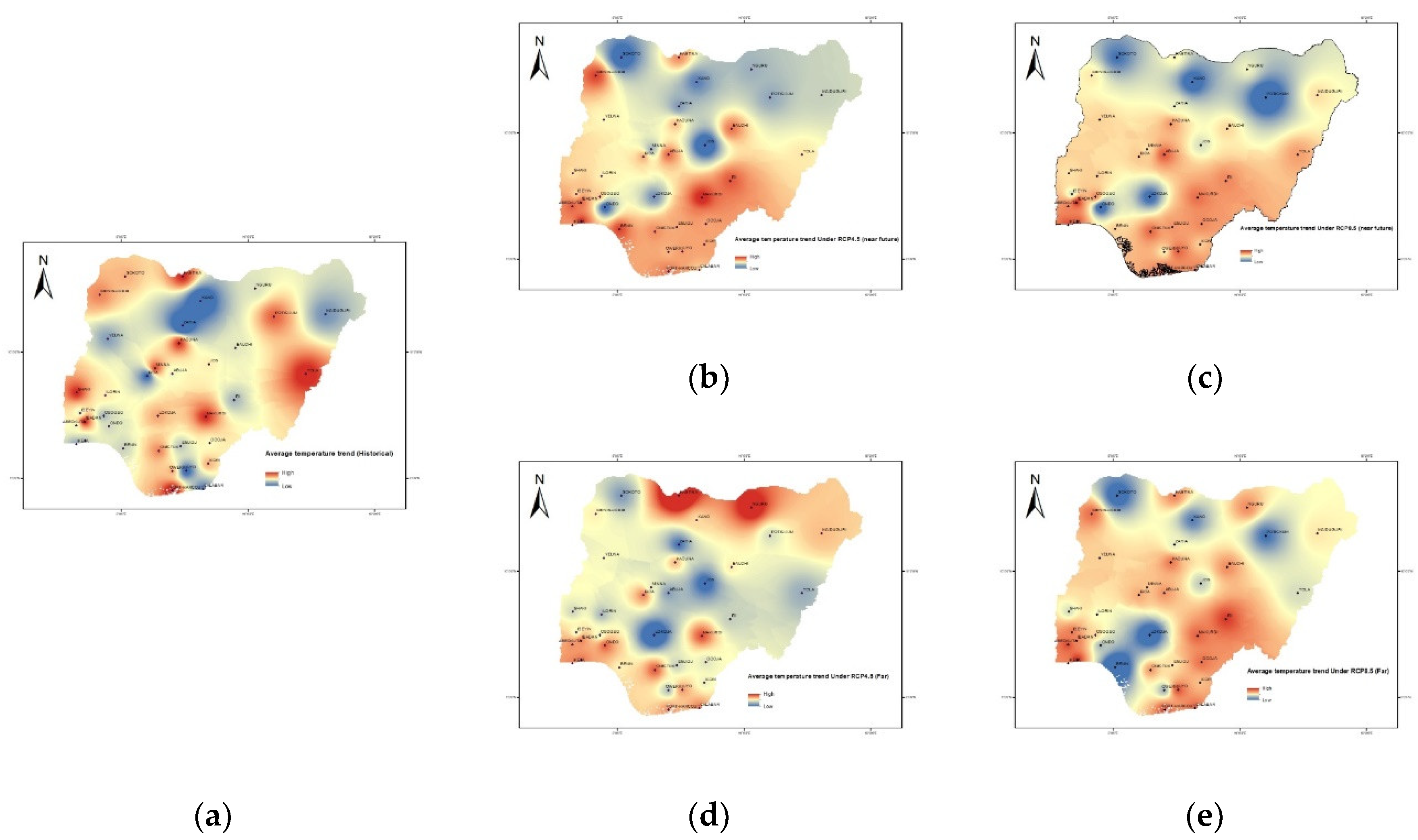
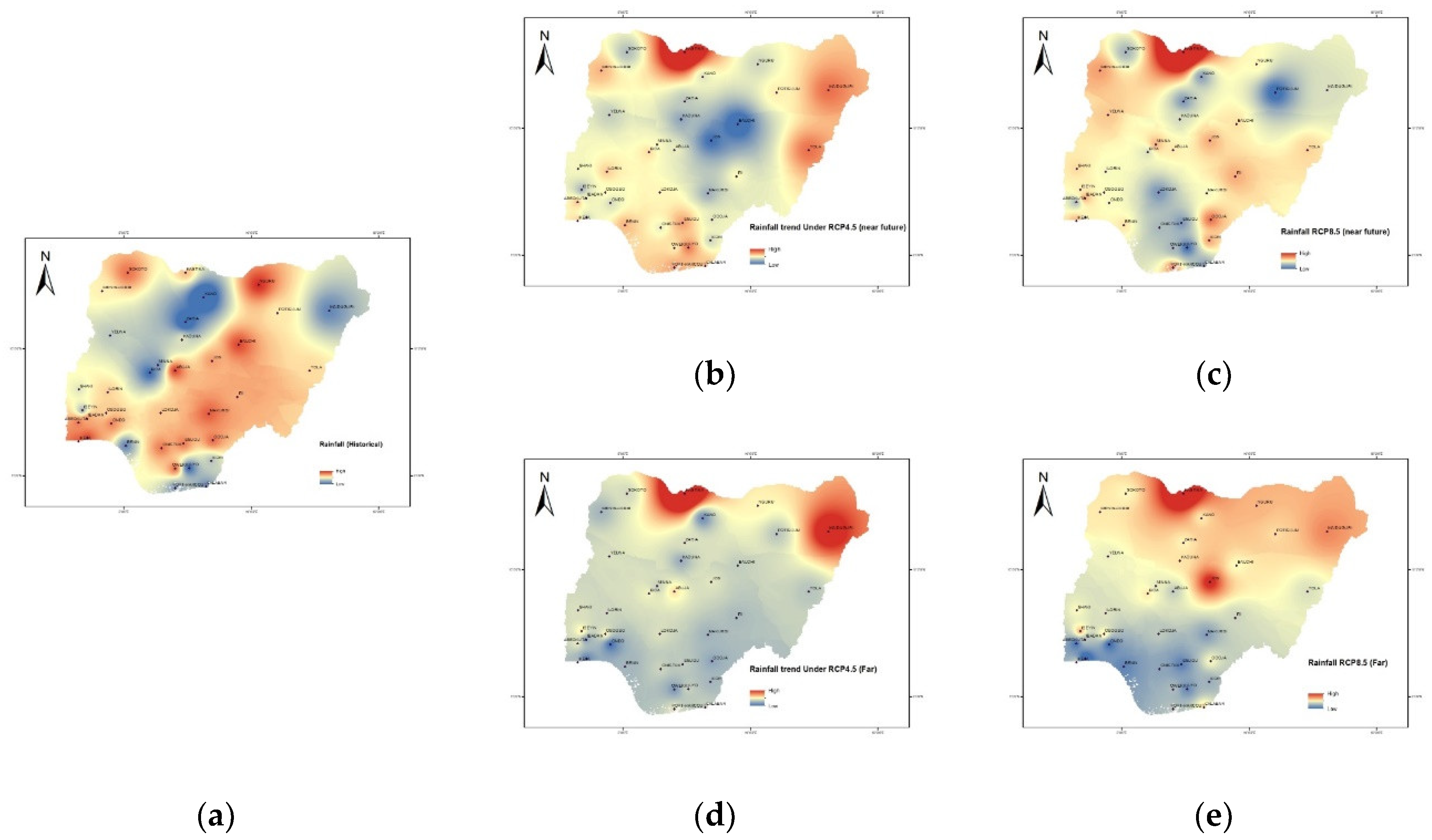
The Mann-Kendall (M-K) trend test is utilized to measure the changes in climatic variables, whether they are increasing or decreasing, over a span of several years in the time series data. In order to identify areas vulnerable to climate change, spatial interpolation was performed for rainfall and mean temperature. Figure 14 and Figure 15 depict the spatial representation of the magnitude of change in mean temperature and annual rainfall across the country respectively. The areas depicted in red represents areas of high magnitude of change while areas in blue represents the low areas. In general, there was no significant change in annual rainfall throughout the country. The historical period showed a negative trend in annual rainfall (reduction in rainfall), with a slight increase projected for the future under the RCP4.5 and RCP8.5 scenarios. The z-values for rainfall ranged from -4.74 to 0.344, with an average value of -1.425 during the historical period. In the near and far future, under RCP 4.5 and RCP 8.5 respectively, the average z-values increased to 0.123, 0.28, 0.39, and 0.32. Similarly, Oguntunde et al. (2017) found that annual rainfall did not exhibit a significant increasing or decreasing trend, but there was an observed increase in variability, and more extreme weather events. The coastal regions and certain parts of the Sudan area in the north are experiencing the most significant reductions in rainfall. This finding contradicts the assertion made by Akinbile, et al., (2019) which suggested a negative linear correlation between rainfall quantity and latitude, stating that rainfall decreases with increasing latitude away from the Atlantic Ocean due to latitudinal zonality in precipitation. However, it is possible that this discrepancy is a result of limited data used for their spatial analysis. Climate change has the potential to modify global and regional atmospheric circulation patterns, leading to increased variability in rainfall. This can result in more frequent and intense extreme weather events, such as droughts and heavy rainfall events. Coastal areas, due to their proximity to the ocean and potential interactions with changing weather patterns, may be particularly vulnerable to these variations in rainfall. Consequently, this heightened variability can contribute to an overall reduction in the trend of annual rainfall even in the coastal areas. In contrast, for future scenarios under RCP4.5 and RCP8.5, these vulnerable areas show slight increases in annual rainfall amounts.
There is a significant increase in mean temperature values in the country for the historical as well as the future case scenarios in agreement with the general axiom of global warming and climate change. The spatial representation historical change in mean temperature does not show a distinction between the pattern in the southern and northern region, however there is observable lowering of the magnitude of change in the future under the RCP4.5 case scenario. Contrariwise, under the RCP8.5 scenario greater areas experiences significant increase in the mean temperature. Quantifying temporal variability of change in mean temperature may be less apparent than rainfall variability as rainfall tends to be more spatially heterogeneous, climate change can also influence temperature variability. As the average temperature may increase, there can also be greater fluctuations in temperature, including more extreme hot and cold events. The z-values for average temperature ranged from 5.11 to 7.52, with an average value of 6.52 during the historical period. In the near and far future, under RCP 4.5 z-values decreases to 4.6570 and 2.604 a testament to the effect of a “stabilization case scenario”. While the average z-values remain largely unchanged under the “business-as-usual case scenario” with an average z-value of 6.063 and 5.910 for the near and future temporal time scales respectively. Increasing temperature can have significant implications for agriculture in Nigeria as it may negatively affect crop growth, reduce yields, and impact livestock productivity. Also, the increasing temperature can disrupt the local water availability as higher temperatures increase evaporation rates, leading to greater water loss from surface water bodies and soil moisture

4. Conclusions

This article presents the results of an analysis of historical as well as future meteorological information and trends in temperature and rainfall across different agroecological zones of Nigeria. ANN is employed in improving the accuracy of downscaled GCM models over Nigeria. It emphasizes the need to improve predictability of climate models, which can impact climate impact assessments. Model validation is crucial to ensure model reliability. The study explores some multimodal ensemble techniques to improve climate projections but acknowledges their limitations in capturing complex climate system interactions. ECMs are displayed as a robust approach, pooling multiple models to provide more accurate climate projections. The article underscores the importance of precise climate modelling in data-scarce regions like Africa and offers insights into the challenges and opportunities in the field.
The performance of the ensemble techniques was assessed using three modelling error metrics. Overall, ANN-ECMs better simulates the actuality of meteorological information better than MLR and AM method or any single GCM for the region. In addition, the RMSE show that ECMS can reduce the probability of large errors in climate model projections. By better predicting the amplitude and capturing the spatial pattern of meteorological information. The ANN ensemble method increased the reliability of GCM for wide range impact assessment. And reiterates the importance of the multi-model approach for improving robustness of climate change projections. It is evident that there is still little understanding and discretization of the processes that are responsible for the original climate model errors for the region. Hence, the need for investigations into source of uncertainties in GCMs over the region is imperative to enable climate models better represent the more intricate climate of the African continent. These findings aid understanding and monitoring climate trends to assess their potential impacts on sectors such as agriculture, water resources, and energy. Further research is needed to explore the specific implications of these changing climate patterns on various crops and ecosystems within each agroecological zone of the country.

Supplementary Materials

The following supporting information can be downloaded at the website of this paper posted on Preprints.org.

Author Contributions

For research articles with several authors, a short paragraph specifying their individual contributions must be provided. The following statements should be used “Conceptualization, D.A.O and A.T.O.; software, D.A.O and A.T.O.; formal writing—review and editing, D.A.O and K.A.A; visualization, D.A.O and A.T.O.; supervision, K.A.A. All authors have read and agreed to the published version of the manuscript.”

Acknowledgments

The Authors acknowledge the role of Landmark University, Omu-Aran in sponsoring the research publication.

Conflicts of Interest

The authors declare no conflicts of interest.

References

  1. Adedapo, A. (2020). Trend Analysis of Temperature and Humidity in Kwara State, Nigeria. Journal of Environmental Geography, 13(3–4). [CrossRef]
  2. Adenle, A., Eckert, S., Ifejika Speranza, C., Oluwatola, A., & Ellison, D. (2020). Human-induced land degradation dominance in the Nigerian Guinea Savannah between 2003 – 2018. Remote Sensing Applications: Society and Environment, 19, 100360. [CrossRef]
  3. Ajetomobi, J., Ajiboye, A., & Rashid, H. (2011). IMPACTS OF CLIMATE CHANGE ON RICE AGRICULTURE IN NIGERIA [IMPACTOS DEL CAMBIO CLIMÁTICO EN. Tropical and Subtropical Agroecosystems, 14, 613–622.
  4. Akinbile, C. O., Akinlade, G. M., & Abolude, A. T. (2015). Trend analysis in climatic variables and impacts on rice yield in Nigeria. Journal of Water and Climate Change, 6(3). [CrossRef]
  5. Akinbile, C., Ogunmola, O., Abolude, A., & Akande, S. (2019). Trends and spatial analysis of temperature and rainfall patterns on rice yields in Nigeria. Atmospheric Science Letters. [CrossRef]
  6. Akpenpuun, T. D., & Busari, R. A. (2018). Impact of climate on the yield of major tuber crops in Kwara State, Nigeria. Global Journal of Agricultural Sciences, 16(1). [CrossRef]
  7. Atiah, W. A., Amekudzi, L. K., Aryee, J. N. A., Preko, K., & Danuor, S. K. (2020). Validation of satellite and merged rainfall data over Ghana, West Africa. Atmosphere, 11(8). [CrossRef]
  8. Attogouinon, A., Lawin, A., N’Tcha M’Po, Y., & Houngue, R. (2017). Extreme Precipitation Indices Trend Assessment over the Upper Oueme River Valley-(Benin). Hydrology, 4, 36. [CrossRef]
  9. Ayanlade, A. (2009). Seasonal rainfall variability in Guinea Savanna part of Nigeria: A GIS approach. International Journal of Climate Change Strategies and Management, 1(3). [CrossRef]
  10. Battisti, R., Sentelhas, P. C., & Boote, K. J. (2017). Inter-comparison of performance of soybean crop simulation models and their ensemble in southern Brazil. Field Crops Research, 200. [CrossRef]
  11. Bello, A., Bashir, Bello, Y., Adebayo, A. A., & Abubakar. (2020). ANALYSIS OF RAINFALL… ANALYSIS OF RAINFALL AND TEMPERATURE CHANGES IN GOMBE STATE, NIGERIA. FJS FUDMA Journal of Sciences (FJS (Vol. 4).
  12. Bello, N. J. (1998). Evidence of climate change based on rainfall records in Nigeria. Weather, 53(12). [CrossRef]
  13. Bichet, A., & Diedhiou, A. (2018). West African Sahel has become wetter during the last 30 years, but dry spells are shorter and more frequent. Climate Research, 75(2), 155–162. [CrossRef]
  14. Buis, A. (2020). Milankovitch (Orbital) Cycles and Their Role in Earth’s Climate – Climate Change: Vital Signs of the Planet. Nasa Global Cimate Change.
  15. Chen, H., Xu, C. Y., & Guo, S. (2012). Comparison and evaluation of multiple GCMs, statistical downscaling and hydrological models in the study of climate change impacts on runoff. Journal of Hydrology, 434–435. [CrossRef]
  16. Chokkavarapu, N., & Mandla, V. R. (2019). Comparative study of GCMs, RCMs, downscaling and hydrological models: a review toward future climate change impact estimation. In SN Applied Sciences (Vol. 1, Issue 12). [CrossRef]
  17. Crawford, J., Venkataraman, K., & Booth, J. (2019). Developing climate model ensembles: A comparative case study. Journal of Hydrology, 568. [CrossRef]
  18. Demessie, S. F., Dile, Y. T., Bedadi, B., Gashaw, T., & Tefera, G. W. (2023). “Evaluations of regional climate models for simulating precipitation and temperature over the Guder sub-basin of Upper Blue Nile Basin, Ethiopia.” Modeling Earth Systems and Environment. [CrossRef]
  19. Dieterich, C., Schimanke, S., Wang, S., Väli, G., & Liu, Y. (2013). Evaluation of the SMHI coupled atmosphere-ice-ocean model RCA4-NEMO. https://www.diva-portal.org/smash/record.jsf?pid=diva2:947918.
  20. Duarte, Y. C. N., & Sentelhas, P. C. (2020). NASA/POWER and DailyGridded weather datasets—how good they are for estimating maize yields in Brazil? International Journal of Biometeorology, 64(3). [CrossRef]
  21. Dunbar, O. R. A., Garbuno-Inigo, A., Schneider, T., & Stuart, A. M. (2021). Calibration and Uncertainty Quantification of Convective Parameters in an Idealized GCM. Journal of Advances in Modeling Earth Systems, 13(9). [CrossRef]
  22. Emeribe, C. N., Uwadia, N. O., Fasipe, O. A., & E. S., I. (2017). Inter-Decadal Nature of Rainfall Character Over Sudano-Sahel, North-West Nigeria. African Research Review, 11(4). [CrossRef]
  23. Gbode, I. E., Adeyeri, O. E., Menang, K. P., Intsiful, J. D. K., Ajayi, V. O., Omotosho, J. A., & Akinsanola, A. A. (2019). Observed changes in climate extremes in Nigeria. Meteorological Applications, 26(4). [CrossRef]
  24. Ghadirnezhad, R., & Fallah, A. (2014). Temperature effect on yield and yield components of different rice cultivars in flowering stage. International Journal of Agronomy, 2014. [CrossRef]
  25. Gnitou, G. T., Ma, T., Tan, G., Ayugi, B., Nooni, I. K., Alabdulkarim, A., & Tian, Y. (2019). Evaluation of the rossby centre regional climate model rainfall simulations over west africa using large-scale spatial and temporal statistical metrics. Atmosphere, 10(12). [CrossRef]
  26. Guo, D., & Wang, H. (2016). Comparison of a very-fine-resolution GCM with RCM dynamical downscaling in simulating climate in China. Advances in Atmospheric Sciences, 33(5). [CrossRef]
  27. Gyamfi, C., Tindan, J. Z. O., & Kifanyi, G. E. (2021). Evaluation of CORDEX Africa multi-model precipitation simulations over the Pra River Basin, Ghana. Journal of Hydrology: Regional Studies, 35, 100815. [CrossRef]
  28. Handoko, U., Boer, R., Aldrian, E., Latifah, A. L., Dasanto, B. D., Apip, A., & Misnawati, M. (2019). Comparison Performance of the Multi-Regional Climate Model (RCM) in Simulating Rainfall and Air Temperature in Batanghari Watershed. Aceh International Journal of Science and Technology, 8(2). [CrossRef]
  29. Harris, I., Osborn, T. J., Jones, P., & Lister, D. (2020). Version 4 of the CRU TS monthly high-resolution gridded multivariate climate dataset. Scientific Data, 7(1), 109. [CrossRef]
  30. Hernández-Díaz, L., Laprise, R., Sushama, L., Martynov, A., Winger, K., & Dugas, B. (2013). Climate simulation over CORDEX Africa domain using the fifth-generation Canadian Regional Climate Model (CRCM5). Climate Dynamics, 40(5), 1415–1433. [CrossRef]
  31. Ibitolu, H. A., & Balogun, I. (2019). An assessment of drought in Northern Nigeria using spatiotemporal remote sensing data. In Proceedings of the International Astronautical Congress, IAC (Vol. 2019-October).
  32. 32. IPCC. (2014). IPCC’s Fifth assessment Report: Impacts, Adaptation, and Vulnerability. IPCC WG2.
  33. Kumi, N., Abiodun -, B. J., Abdi, A. M., Seaquist, J., Tenenbaum, D. E., Porkka, M., … Gordon, L. J. (2021). Is wetter better? Exploring agriculturally-relevant rainfall characteristics over four decades in the Sahel. Environmental Research Letters, 16(3), 035002. Retrieved 29 August 2022 from. [CrossRef]
  34. Jang, D. (2021). An Application of ANN Ensemble for Estimating of Precipitation Using Regional Climate Models. Advances in Civil Engineering, 2021. [CrossRef]
  35. Jose, D. M., Vincent, A. M., & Dwarakish, G. S. (2022). Improving multiple model ensemble predictions of daily precipitation and temperature through machine learning techniques. Scientific Reports, 12(1). [CrossRef]
  36. Kim, C. G., Park, J., & Cho, J. (2018). Future Climate Change Impact Assessment of Chungju Dam Inflow Considering Selection of GCMs and Downscaling Technique. Journal of Climate Change Research, 9(1). [CrossRef]
  37. Lange, S., & Vinke, K. (2021). Climate Risk Profile: Sahel * Summary. Retrieved 7 September 2022 from.
  38. le Blanc, D., & Perez, R. (2008). The relationship between rainfall and human density and its implications for future water stress in Sub-Saharan Africa. Ecological Economics, 66(2–3). [CrossRef]
  39. Lim, C. M., Yhang, Y. bin, & Ham, S. (2019). Application of GCM bias correction to RCM simulations of East Asian winter climate. Atmosphere, 10(7). [CrossRef]
  40. 40. Maraun, Douglas, Theodore G. Shepherd, Martin Widmann, Guiseppe Zappa, Daniel Walton, Jose M. Guitierrex, Stefan Hagemann, (2017). Towards Process-Informed Bias Correction of Climate Change Simulations. Nature Climate Change 7 (11):764-73.
  41. Mascaro, G., White, D. D., Westerhoff, P., & Bliss, N. (2015). Performance of the CORDEX-Africa regional climate simulations in representing the hydrological cycle of the Niger River basin. Journal of Geophysical Research: Atmospheres, 120(24), 12425–12444. [CrossRef]
  42. Meenal, R., Michael, P. A., Pamela, D., & Rajasekaran, E. (2021). Weather prediction using random forest machine learning model. Indonesian Journal of Electrical Engineering and Computer Science, 22(2). [CrossRef]
  43. Mereu, V., Carboni, G., Gallo, A., Cervigni, R., & Spano, D. (2015). Impact of climate change on staple food crop production in Nigeria. Climatic Change, 132(2). [CrossRef]
  44. Mertz, O., D’haen, S., Maiga, A., Moussa, I. B., Barbier, B., Diouf, A., … Dabi, D. (2012). Climate variability and environmental stress in the Sudan-Sahel zone of West Africa. Ambio, 41(4). [CrossRef]
  45. 45. Nissan, Hannah, Lisa Goddard, Erin Coughlan de Perez, John Furlow, Walter Baethgen, Madeleine C. Thomson, and Simon J. Mason. (2019). On the Use and Misuse of Climate Change Projections in International Development. WIRES Climate Change 10 (3): e579.. [CrossRef]
  46. Odigwe, M., Efe, S. I., & Atubi, A. O. (2020). A Statistical Discourse of the Climate of the Niger Delta Region of Nigeria. Journal of Management and Social Science Research, 1(1/2). [CrossRef]
  47. Ogungbenro, S. B., & Morakinyo, T. E. (2014). Rainfall distribution and change detection across climatic zones in Nigeria. Weather and Climate Extremes, 5(1). [CrossRef]
  48. Ogunjo, S., Ife-Adediran, O., Owoola, E., & Fuwape, I. (2019). Quantification of historical drought conditions over different climatic zones of Nigeria. Acta Geophysica, 67(3). [CrossRef]
  49. Ogunrinde, A. T., Oguntunde, P. G., Akinwumiju, A. S., & Fasinmirin, J. T. (2019). Analysis of recent changes in rainfall and drought indices in Nigeria, 1981–2015. Hydrological Sciences Journal. [CrossRef]
  50. Ogunrinde, A. T., Oguntunde, P. G., Fasinmirin, J. T., & Akinwumiju, A. S. (2020). Application of artificial neural network for forecasting standardized precipitation and evapotranspiration index: A case study of Nigeria. Engineering Reports, 2(7), e12194. [CrossRef]
  51. Ogunrinde, A. T., Olasehinde, D. A., & Olotu, Y. (2020). Assessing the sensitivity of standardized precipitation evapotranspiration index to three potential evapotranspiration models in Nigeria. Scientific African, 8. [CrossRef]
  52. Oguntunde, P. G., Abiodun, B. J., & Lischeid, G. (2017). Impacts of climate change on hydro-meteorological drought over the Volta Basin, West Africa. Global and Planetary Change. [CrossRef]
  53. Oguntunde, P. G., Lischeid, G., & Abiodun, B. J. (2017). Impacts of climate variability and change on drought characteristics in the Niger River Basin, West Africa. Stochastic Environmental Research and Risk Assessment 2017 32:4, 32(4), 1017–1034. Retrieved 26 July 2021 from. [CrossRef]
  54. Ojo, D., Connaughton, M., Kintomo, A., Olajide-Taiwo, L. O., & Afolayan, S. (2011). Assessment of irrigation systems for dry season vegetable production in urban and peri-urban zones of Ibadan and Lagos, Southwestern Nigeria. African Journal of Agricultural Research, 6.
  55. Olaniran, O. J. (1986). On the classification of tropical climates for the study of regional climatology: Nigeria as a case study. Geografiska Annaler, Series A. [CrossRef]
  56. Onah, E. I. (2020). Nigeria: A Country Profile. Journal of International Studies. [CrossRef]
  57. Pohl, B., & Douville, H. (2011). Diagnosing GCM errors over West Africa using relaxation experiments. Part II: Intraseasonal variability and African easterly waves. Climate Dynamics, 37(7–8). [CrossRef]
  58. Pausata, F. S. R., Gaetani, M., Messori, G., Berg, A., Maia de Souza, D., Sage, R. F., & deMenocal, P. B. (2020). The Greening of the Sahara: Past Changes and Future Implications. One Earth, 2(3), 235–250. Retrieved 29 August 2022 from. [CrossRef]
  59. Rogelj, J., Meinshausen, M., & Knutti, R. (2012). Global warming under old and new scenarios using IPCC climate sensitivity range estimates. Nature Climate Change, 2(4), 248–253. [CrossRef]
  60. Raju, K. S., & Kumar, D. N. (2020). Review of approaches for selection and ensembling of GCMS. In Journal of Water and Climate Change (Vol. 11, Issue 3). [CrossRef]
  61. Rezaie-Balf, M., Kim, S., Fallah, H., & Alaghmand, S. (2019). Daily river flow forecasting using ensemble empirical mode decomposition based heuristic regression models: Application on the perennial rivers in Iran and South Korea. Journal of Hydrology, 572. [CrossRef]
  62. Rowell, David P., Catherine A. Senior, Michael Vellinga, and Richard J. Graham (2016). Can Climate Projection Uncertainty Be Constrained Over Africa using Metrics of Contemporary Performance? Climate Change 134 (4):621-33. [CrossRef]
  63. Salami, A. W., Olanlokun, O., Salami, A. W., Mohammed, A. A., Abdulmalik, Z. H., & Olanlokun, O. K. (2014). Trend Analysis of Hydro-meteorological Variables using the Mann-Kendall Trend Test: Application to the Niger River and the Benue Sub-Basins in Nigeria. International Journal of Technology, 2, 100–110. Retrieved 30 November 2021 from. [CrossRef]
  64. Sallaba, F., Olin, S., Engström, K., Abdi, A. M., Boke-Olén, N., Lehsten, V., … Seaquist, J. W. (2017). Future supply and demand of net primary production in the Sahel. Earth System Dynamics, 8(4). [CrossRef]
  65. Schmidli, J., Frei, C., & Vidale, P. L. (2006). Downscaling from GCM precipitation: A benchmark for dynamical and statistical downscaling methods. International Journal of Climatology, 26(5). [CrossRef]
  66. Seager, Richard Naomi Henderson, and Mark Cane (2022). Persistent Discrepancies between Observed and Modeled Trends in the Tropical Pacific Ocean. Journal of Climate 35(14):4571-84. [CrossRef]
  67. Siddig, K., Stepanyan, D., Wiebelt, M., Grethe, H., & Zhu, T. (2020). Climate change and agriculture in the Sudan: Impact pathways beyond changes in mean rainfall and temperature. Ecological Economics, 169. [CrossRef]
  68. Sharma, C., Ojha, C. S. P., Shukla, A. K., Pham, Q. B., Linh, N. T. T., Fai, C. M., Loc, H. H., & Dung, T. D. (2019). Modified approach to reduce GCM bias in downscaled precipitation: A study in Ganga River Basin. Water (Switzerland), 11(10). [CrossRef]
  69. Shrivastava, G., Karmakar, S., Kumar Kowar, M., & Guhathakurta, P. (2012). Application of Artificial Neural Networks in Weather Forecasting: A Comprehensive Literature Review. International Journal of Computer Applications, 51(18). [CrossRef]
  70. Stouffer, D. B., Curtsdotter, A., Banks, H. T., Banks, J. E., Jonsson, M., Jonsson, T., Laubmeier, A. N., & Bommarco, R. (2019). All ecological models are wrong, but some are useful. Journal of Animal Ecology, 88(2). [CrossRef]
  71. Stute, M., Clement, A., & Lohmann, G. (2001). Global climate models: Past, present, and future. Proceedings of the National Academy of Sciences of the United States of America, 98(19). [CrossRef]
  72. Taylor, S. (2005). Taylor Diagram Primer Karl E. Taylor. Work. Pap, January.
  73. Tealab, A., Hefny, H., & Badr, A. (2017). Forecasting of nonlinear time series using ANN. Future Computing and Informatics Journal, 2(1). [CrossRef]
  74. Tunde, A. M., Adeleke, E. A., & Adeniyi, E. E. (2013). Impact of climate variability on human health in Ilorin, Nigeria. Environment and Natural Resources Research. [CrossRef]
  75. Vaittinada Ayar, P., Vrac, M., & Mailhot, A. (2021). Ensemble bias correction of climate simulations: preserving internal variability. Scientific Reports, 11(1). [CrossRef]
  76. van Vuuren, D. P., Edmonds, J., Kainuma, M., Riahi, K., Thomson, A., Hibbard, K., … Rose, S. K. (2011). The representative concentration pathways: An overview. Climatic Change. [CrossRef]
  77. Washington, R., Harrison, M., Conway, D., Black, E., Challinor, A., Grimes, D., Jones, R., Morse, A., Kay, G., & Todd, M. (2006). African climate change: Taking the shorter route. Bulletin of the American Meteorological Society, 87(10). [CrossRef]
  78. Willmott, C. J., & Matsuura, K. (2005). Advantages of the mean absolute error (MAE) over the root mean square error (RMSE) in assessing average model performance. Climate Research, 30(1), 79–82. [CrossRef]
  79. World Bank. (2015). Climate and Health country Profile - 2015 Nigeria. World Bank Global Health Expenditure Database United Nations Development Programme Human Development Reports. http://apps.who.int.ezproxy.lib.gla.ac.uk/iris/bitstream/10665/246140/1/WHO-FWC-PHE-EPE-15.40-eng.pdf.
  80. Yang, X., Xie, X., Liu, D. L., Ji, F., & Wang, L. (2015). Spatial Interpolation of Daily Rainfall Data for Local Climate Impact Assessment over Greater Sydney Region. Advances in Meteorology, 2015. [CrossRef]
  81. Xu, Z., Han, Y., & Yang, Z. (2019). Dynamical downscaling of regional climate: A review of methods and limitations. In Science China Earth Sciences (Vol. 62, Issue 2). [CrossRef]
  82. Xu, Z., & Yang, Z. L. (2015). A new dynamical downscaling approach with GCM bias corrections and spectral nudging. Journal of Geophysical Research, 120(8). [CrossRef]
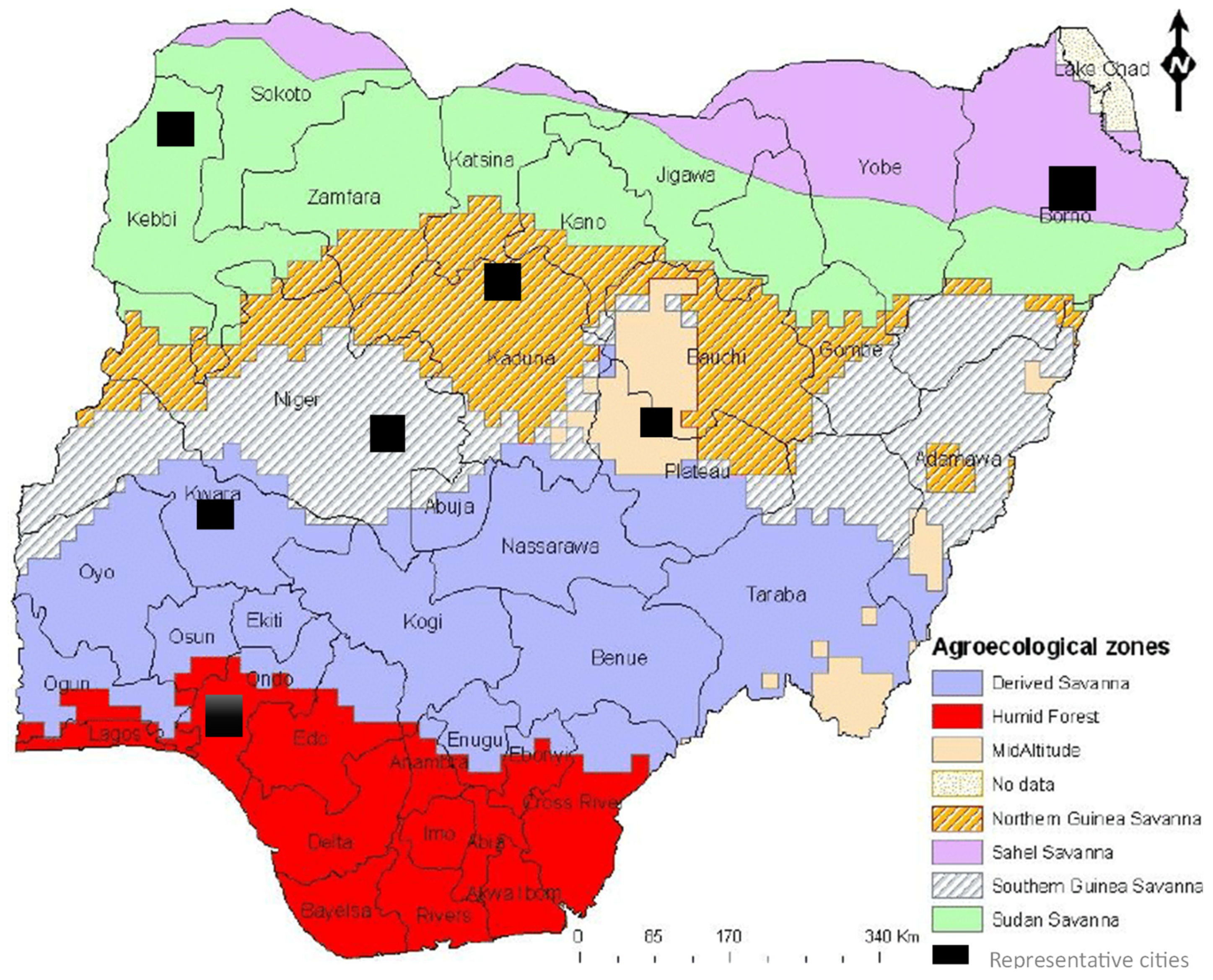
Figure 1. The study area showing the agroecological Zones of Nigeria (Adapted from Mereu et al., 2015).
Preprints 95596 g001
Figure 3. SAS Meterological Summary for (a) Mean temperature and (b) Rainfall.
Preprints 95596 g003
Figure 4. SUS Meterological Summary for (a) Mean temperature and (b) Rainfall.
Preprints 95596 g004
Figure 5. NGS Meterological Summary for (a) Mean temperature and (b) Rainfall.
Preprints 95596 g005
Figure 6. SGS Meterological Summary for (a) Mean temperature and (b) Rainfall.
Preprints 95596 g006
Figure 7. DRS Meterological Summary for (a) Mean temperature and (b) Rainfall.
Preprints 95596 g007
Figure 8. HMF Meterological Summary for (a) Mean temperature and (b) Rainfall.
Preprints 95596 g008
Figure 9. Taylor diagram displaying statistical comparison betweem GCMs and CRU for Rainfall for the years 1950-1994 at the Maiduguri Station.
Preprints 95596 g009
Figure 14. Changes in Mean Temperature. (a) Trend in Average temperature (historical); (b) Trend in Average temperature Under RCP4.5 (near future); (c) Trend in Average temperature Under RCP8.5 (near future); (d) Trend in Average temperature Under RCP4.5 (far future); (e) Trend in Average temperature Under RCP8.5 (far future).
Preprints 95596 g014
Figure 15. Changes in Annual Rainfall. (a) Trend in Rainfall (historical); (b) Trend in Rainfall Under RCP4.5 (near future); (c) Trend in Rainfall Under RCP8.5 (near future); (d) Trend in Rainfall Under RCP4.5 (far future); (e) Trend in Rainfall Under RCP8.5 (far future).
Preprints 95596 g015
Table 1. List of GCM model simulations used in this study.
S/N Modeling Center or Institute Resolution of GCM GCM Output Name RCM name
1 Canadian Centre for Climate Modelling and Analysis (CCCMA) 2.8o x 2.8o CCCCMA-CanESM2 CCCMA-RCA4
2 Centre National de Recherches Météorologiques (CNRM) 1.4o x 1.4o CNRM-CERFACS-CNRM-CM5 CNRM-RCA4
3 NOAA Geophysical Fluid Dynamics Laboratory
(NOAA-GDFL)
2.5o x 2.0o

NOAA-GDFL-GDFL-ESM2M NOAA-RCA4
4 EC-EARTH consortium (ICHEC-EC)
1.9o x 1.3o
ICHEC-EC-EARTH ICHEC-RCA4
5 Atmosphere and Ocean Research Institute (The University of Tokyo), National Institute for Environmental Studies, and Japan Agency for Marine-Earth Science and Technology 1.4o x 1.4o MIROC-MIROC5 MIROC-RCA4
6 Max-Planck-Institut für Meteorologie (Max Planck Institute for Meteorology) 1.9o x 1.9o

MPI-M-MPI-ESM-LR MPI-RCA4
7 Norwegian Climate Centre 2.5o x 1.9o
NCC-NorESM1-M NCC-RCA4
Table 2. Correlation value and its criteria displaying similarities in models’ pattern (Handoko, et. al., 2019).
Correlation Criteria
0.9 to 1.0 Very high correlation
0.7 to 0.9 High correlation
0.5 to 0.7 Moderate correlation
0.3 to 0.5 Low correlation
0.0 to 0.3 Correlation can be ignored
Table 4. Monthly M-K trend analysis of rainfall and mean temperature in the agroecological zones of Nigeria.
Zone Test variable Jan Feb Mar Apr May Jun Jul Aug Sep Oct Nov Dec Average
SAS Z- value Mean Temperature -0.83 1.62 2.94 5.11 5.11 5.59 4.67 4.10 3.98 4.99 2.94 1.08 5.94
Rainfall Na Na Na 0.38 -0.42 0.93 0.14 -0.77 0.47 1.34 Na Na -0.50
Sen’s slope Mean Temperature 0.00 0.01 0.02 0.03 0.02 0.02 0.02 0.02 0.01 0.02 0.02 0.01 0.01
Rainfall Na Na Na 0.00 -0.05 0.27 0.05 -0.24 0.15 0.10 Na Na -0.31
SUS Z- value Mean Temperature 0.33 1.99 4.45 5.88 4.33 3.73 5.23 4.67 5.33 4.92 4.33 2.30 6.93
Rainfall Na 2.22 0.44 0.52 -0.12 -0.03 -1.40 -0.97 -1.06 1.66 3.32 Na -2.47
Sen’s slope Mean Temperature 0.00 0.02 0.02 0.02 0.02 0.02 0.02 0.02 0.02 0.02 0.02 0.01 0.02
Rainfall 0.00 0.00 0.00 0.06 -0.02 -0.01 -0.40 -0.28 -0.28 0.26 0.00 0.00 -1.67
NGS Z- value Mean Temperature 0.45 1.93 4.21 5.17 4.78 3.73 4.74 4.60 4.71 4.67 3.98 1.93 6.64
Rainfall Na 2.52 -2.68 0.33 0.04 0.93 -1.23 0.42 -0.57 1.87 1.66 Na 0.00
Sen’s slope Mean Temperature 0.00 0.00 0.02 0.02 0.02 0.01 0.02 0.02 0.02 0.02 0.02 0.01 0.02
Rainfall 0.00 0.00 -0.06 0.06 0.01 0.18 -0.30 0.09 -0.20 0.45 0.00 0.00 0.01
SGS Z- value Mean Temperature 1.15 2.90 5.64 5.07 4.17 4.25 4.69 4.32 4.66 4.84 5.00 2.98 6.45
Rainfall -1.22 0.83 -2.32 -0.70 0.12 0.80 -1.33 1.33 -1.18 0.34 -0.75 Na 0.12
Sen’s slope Mean Temperature 0.01 0.01 0.02 0.02 0.01 0.01 0.01 0.01 0.01 0.01 0.02 0.01 0.01
Rainfall 0.00 0.00 -0.18 -0.14 0.02 0.16 -0.37 0.45 -0.31 0.09 0.00 0.00 0.08
DRS Z- value Mean Temperature 2.19 4.36 5.73 4.25 4.26 4.24 4.65 4.27 3.98 4.29 5.42 4.31 6.13
Rainfall 0.06 1.46 -2.45 -1.23 -0.68 0.64 -0.94 2.13 1.37 0.44 -0.33 0.01 0.10
Sen’s slope Mean Temperature 0.01 0.02 0.02 0.02 0.01 0.01 0.01 0.01 0.01 0.01 0.02 0.02 0.01
Rainfall 0.00 0.05 -0.31 -0.26 -0.12 0.10 -0.20 0.64 0.28 0.13 -0.01 0.00 0.09
HMF Z- value Mean Temperature 2.40 4.88 5.19 3.73 4.55 4.84 4.82 4.33 4.07 4.19 5.70 4.63 5.93
Rainfall -0.76 0.38 -2.66 -1.26 -0.86 -0.63 -0.56 2.50 2.14 0.32 -1.08 -0.93 0.35
Sen’s slope Mean Temperature 0.01 0.02 0.02 0.01 0.01 0.01 0.01 0.01 0.01 0.01 0.02 0.02 0.01
Rainfall -0.03 0.05 -0.49 -0.33 -0.17 -0.17 0.74 1.10 0.93 0.09 -0.15 -0.06 0.38
ALT Z- value Mean Temperature 0.41 2.12 4.09 5.45 5.44 4.39 4.81 4.81 4.42 4.90 4.06 1.80 7.06
Rainfall 1.74 2.27 -1.89 -0.34 0.02 0.40 -0.39 1.57 -1.21 1.72 0.10 Na -0.09
Sen’s slope Mean Temperature 0.00 0.01 0.02 0.02 0.02 0.01 0.02 0.01 0.01 0.01 0.02 0.01 0.01
Rainfall 0.00 0.01 -0.14 -0.07 0.01 0.08 -0.11 0.38 -0.31 0.32 0.00 0.00 -0.10
Disclaimer/Publisher’s Note: The statements, opinions and data contained in all publications are solely those of the individual author(s) and contributor(s) and not of MDPI and/or the editor(s). MDPI and/or the editor(s) disclaim responsibility for any injury to people or property resulting from any ideas, methods, instructions or products referred to in the content.
Copyright: This open access article is published under a Creative Commons CC BY 4.0 license, which permit the free download, distribution, and reuse, provided that the author and preprint are cited in any reuse.
Prerpints.org logo

Preprints.org is a free preprint server supported by MDPI in Basel, Switzerland.

Subscribe

© 2024 MDPI (Basel, Switzerland) unless otherwise stated