
Submitted:
05 January 2024
Posted:
05 January 2024
You are already at the latest version
Abstract
Seawater density is an important physical property in oceanography that affects the accuracy of calculations such as gravity fields and tidal potentials, and the calibration of acoustic and optical oceanographic sensors. In related studies, constant density values are frequently used, which can introduce significant errors. Therefore, this study employs a basic convolutional neural network model to construct a comprehensive model showing the seawater density distribution across the globe. The model takes into account depth, latitude, longitude, and month as inputs. Numerous real seawater datasets were used to train the model, and it has been shown that the model has an absolute mean error and root mean square error of less than 2 kg/m3 in 99% of the test set samples. The model effectively demonstrates the influence of input parameters on the distribution of seawater density. In this paper, we present a newly developed global model for distributing seawater density which is both comprehensive and accurate, surpassing previous models. The utilization of the model presented in this paper for estimating seawater density can minimize errors in theoretical ocean models and serve as a foundation for designing and analyzing ocean exploration systems.
Keywords:
seawater density
; spatial distribution model of density
; latitude
; Convolutional Neural Network
1. Introduction
Seawater density is a fundamental physical property in the field of oceanography. Using a spatial distribution model for seawater density in the region of interest would significantly decrease errors in gravitational field modeling by using actual density distribution [1]. The effect of seawater density variations on the tidal potential is as large as 2-3 cm in water height equivalent [2]. In comparison to homogeneous seawater, the total speed of a tsunami in a density-stratified seawater is lower [3]. The relationship between the density of seawater and the rise in sea level is amplified within the framework of global warming [4]. Furthermore, seawater density acts as a vital point of reference or compensation value for the calibration and adjustment of ocean sensors [5]. For example, the density of the medium needs to be considered in the sound velocity variation in sonar detection technology [5] and the high-precision optical ocean detection technology [6]. Previous studies have generally regarded seawater density as unvarying, but this notion is inadequate [7]. The density of seawater varies between 995-1070 kg/m3. If a constant density is used in a study, errors will inevitably occur. For instance, using constant density in gravity calculation models can introduce an error of up to 2% [8]. Understanding seawater density distribution can be advantageous for technological advancements in marine applied sciences.
Measuring seawater density directly in situ poses challenges [9]. Instead, seawater temperature, salinity, and depth information can be obtained from marine hydrographic datasets. These datasets can then be used to calculate seawater density with the thermodynamic Equation of Seawater-2010 (TEOS-10) [10]. Accessing these datasets is easy, and shared resources like the World Ocean Database [11] provide valuable sources for marine-related research. The accuracy of TEOS-10 calculations is exceptionally high [12]. However, this approach fails to generate a spatial density model of seawater for the aforementioned investigations.
Research into the global distribution of seawater density is limited. Neutral density γn and neutral surfaces [13] provide an appropriate framework for ocean model calculations and analysis. The sampling points of latitude, longitude, and depth have high resolution. Gladkikh and Tenzer [14] developed a functional model that provides an overall understanding of seawater density distribution based on latitude and depth. Their model employs the absolute latitude yet does not consider the dissimilarities between the Northern and Southern Hemispheres. Furthermore, Talley’s investigation demonstrated that seawater density varies according to latitude and depth, across seasons, and among oceans [15]. The density of seawater undergoes significant variation with changes in depth and latitude. The researchers also accounted for changes in longitude [16] and month [17]. Modeling the effects of these variables set in advance is challenging.
In recent years, oceanographic researchers have employed deep learning to develop seawater temperature, salinity, and tide prediction models [18,19,20], achieving some success. This in turn provides a sound basis for establishing seawater density within the scope of this paper. Compare several classical deep learning methods. The Convolutional Neural Network (CNN) is an optional base used to build a density model. CNNs are deep learning that has shown exceptional proficiency in solving complex nonlinear issues across various industries [21].
This current study strives to fabricate a seawater density distribution model with CNN to introduce the impact of different seasons and ocean regions, thereby creating a more authentic model. The study scrutinizes the model's accuracy as well as its ability to reflect alterations in each given factor. It is hoped that a convenient and accurate mathematical tool can be provided for theoretical studies and detection techniques affected by the density distribution of seawater.
2. Materials and Methods
2.1. Dataset
Data from the Argo program, which forms part of the Global Ocean Observing System, were used to collect oceanic information such as temperature, salinity, pressure, and biogeochemical components [22]. The International Argo Programme and its associated national programs offer these data freely. Most importantly, the Argo dataset was selected for research requirements due to the following reasons [23]. (1) Vertical sampling resolution that is "hybrid" with high-resolution modes at shallower depths or where there is considerable variation in the vertical profile. (2) The majority of the floats operate within a pressure range of up to 2,000 dbar. (3) The geographic distribution of samples offering almost complete ocean coverage. (4) The temperature, salinity, and pressure sensors have high resolution and exhibit good stability.
Data collected from 2017 to 2022 was analyzed, and 'data quality code' options were configured to ensure reliability. The necessary parameters of the dataset are DATE, LATITUDE (degree_north), LONGITUDE (degree_east), PRES (decibar), PSAL (psu), and TEMP (degree_Celsius). Every parameter marked with 'XX_QC=1' indicates good quality control.
The dataset was computed and approximated. Seasonal information was represented by extracting the months from 'DATE'. In-situ density was computed using TEOS-10, after converting practical salinity to absolute salinity and in-situ temperature to conservative temperature. Subsequently, the latitude and longitude were rounded to a resolution of 1°. Note that 'PRES' has not been converted to depth. For consistency, we will use ‘depth’ instead of ‘PRES’. We have excluded a minor portion of the data due to objective factors, such as locations not considered part of the ocean in salinity calculations. The data beyond 2200 dbar has been removed because it is too insignificant for use in the CNN.
The dataset needs to be divided into training, validation, and test sets for input into the neural network. Their respective tasks are debugging parameters, model optimization, and generalization evaluation [24]. The ratio should be approximately 6:2:2. The data from 2017 to 2021 are randomly distributed into training and validation sets at an 8:2 ratio. To ensure the test set has an extensive range of data distributions, we designate the data for the entirety of 2022 as the validation set. Centering and scaling are performed on each variant independently by computing the mean and standard deviation of the samples in the training set. This process is known as standardization. The mean and standard deviation are then stored and utilized for the validation and test sets. This method facilitated the creation of the necessary database.
2.2. CNN Architecture
The network's architecture is outlined in Figure 1. The model's design incorporates a basic structure consisting of two 1D convolutional layers (with two Max pooling layers) and two fully connected layers. The settings, inputs, and outputs for each layer are shown in Figure 1.
Convolutional layers, activation functions, and pooling layers are standard tertiary structures in convolutional networks. The convolutional layer's objective is to extract input data features by performing the convolution operation, reduce network complexity through parameter sharing and local perception to prevent overfitting, and enhance model generalization capability. Rectification involves the application of an activation function to the output of the convolutional layer. The pooling layer primarily simplifies network complexity. The fully connected layer changes the two-dimensional features produced by the convolutional layer into one-dimensional vectors. The book [25] provides a detailed description of each layer's role.
We utilized the fundamental CNN architecture and purposely selected the activation function. The density exhibits an exponential relationship with depth [14,15]. Consequently, we utilized corresponding activation functions following the convolutional layers, namely sigmoid and tanh. Fully connected layers benefit from the nonlinear properties of ReLU.
Sigmoid is defined as:
Sigmoid(x)=1/(1+exp(-x)),
Tanh is defined as:
Tanh(x)=(exp(x)-exp(-x))/(exp(x)+exp(-x)),
ReLU is defined as:
ReLU(x)=max(0,x),
The characteristic curves of the activation functions used are shown in Figure 2.
3. Results
The dataset from 2017 to 2021 serves as both the training and validation sets for the model demonstrated in Figure 1. The model's performance is optimized by adjusting its hyperparameters. Consequently, a CNN model is developed to portray the in-situ seawater density to latitude, longitude, depth, and month. The types and ranges of the input variables are presented in Table 1. The density of seawater in situ is provided by the model output, with data accuracy determined by computer. This paper analyses the model's output error and investigates the impact of each input variable on the output.
The 2022 dataset was utilized to test the model's seawater density estimation capabilities. Using the TEOS-10 equation, the density was calculated as a reference value. The model outputted an estimated density which was then compared to the reference value, and the resulting error was subjected to statistical analysis.
The test set's latitude and longitude positions were derived using the gsw_SA_from_SP function from the TEOS-10 equation, setting in_ocean=1. This criteria ensures that the sample data is not on land, but may encompass inland seas. The error distribution for all the latitude and longitude locations in the test set is shown in Figure 3, comprising absolute mean error (MAE), root mean square error (RMSE), and maximum absolute error (MAXE). The locations with MAE ≥ 2 kg/m3 are marked with red circles in Figure 3a, which account for 0.84% of the sample size of the test set, including the Black Sea, the Sea of Okhotsk, and the Bering Sea. Figure 3b demonstrates that the root mean square error (RMSE) distribution is similar to the MAE distribution in Figure 3a. Locations where the RMSE is at least 2 kg/m3, constituting 1.09% of the test set sample, are similarly marked in Figure 3a by red circles. Figure 3c illustrates that the areas with greater MAXE lie within the low and middle latitudes of the Northern Hemisphere. The red circles pinpoint the locales with MAXE ≥ 5 kg/m3, which are mostly distributed in the continental margin region. MAE < 3.54 kg/m3, RMSE < 3.8 kg/m3, and MAXE < 5.21 kg/m3 in all regions except the Black Sea, which has a special two-layer density structure [26]. It can be deduced that the density calculation of most oceanic regions by the model proposed in this study is highly accurate.
Figure 4 shows the error distribution curves for two other inputs to the model - depth and month. In Figure 4a, the MAE and RMSE for the density corresponding to depth are less than 1.5 kg/m3. The larger errors are mainly in the range of 0-100 dbar. In Figure 4b, the MAE and RMSE of the month corresponding to the density are less than 1 kg/m3. The larger errors are in the October-December range. Based on the distribution of errors in Figure 3, it can be surmised that the model has a large error in estimating the density in the northern hemisphere at low and middle latitudes in winter.
4. Discussion
Previous seawater density distribution models exclusively utilize latitude and depth as independent variables in the density function. This research paper expands on this by incorporating two additional independent variables, longitude and month. Upon conducting a correlation analysis of the dataset, Pearson's correlation coefficients of all seawater densities to depth, latitude, longitude, and month were found to be 0.95, -0.13, 0.083, and -0.017, respectively. The correlation coefficients for densities with inputs at depths less than 200 dbar are 0.52, -0.31, 0.059, and -0.077, respectively. The influence of longitude and month must be factored in for both shallow and deep waters. The significance of accounting for longitude and month in both shallow and deep waters is evident. The function of each independent variable represented in the model is evaluated individually below.
Depth is the variable that correlates most highly with seawater density, among the four independent variables. Figure 5 illustrates the correlation between seawater density and depth, which was calculated using the density model in this study. The curve of seawater density with depth is similar to the mathematical model proposed by Gladkikh and Tenzer [14]. The location selected for this analysis is situated far from the land. When comparing Figure 5a–c, the density increases as latitude increases, but the increment decreases with depth. Each subplot features density profiles from the Atlantic, Indian, and Pacific Oceans. It is noticeable that the Atlantic Ocean displays slightly greater density than the other two oceans in the same latitude region.
Latitude and longitude are both independent variables and their effect on the distribution of seawater density will be analyzed together in Figure 6. The annual average density is calculated without considering the month's effect. Figure 6a displays the density distribution at a depth of 0 dbar, which represents the seawater surface density. The seawater surface density increases with latitude in the range of 1020-1030 kg/m3 when observing latitudinal change. This result aligns with Gladkikh and Tenzer's model [14]. Nevertheless, in the zone of Asia and Europe where they meet the Arctic Ocean (50-180°E, 50°N), the aforementioned density drops beneath 1020 kg/m3 because of the low salinity of the seawater in that vicinity. Furthermore, the distribution outcomes in Figure 6a are akin to those in Talley's Figure 4.19 [15].
Changes in the distribution of seawater density, in terms of the direction of change in longitude, occur mainly at continental margins. Ocean currents change the direction of motion in these regions, allowing the mixing of seawater with temperature and salinity differences at different latitudes and depths. It seems from Figure 6d. Seawater density varies with longitude distribution up to a depth of 500 dbar. Another manifestation of the variation of density with longitude distribution is the difference in density of different oceans separated by land. The main difference is between the North Atlantic and the North Pacific. The density of the seawater in the southern hemisphere is more homogeneous in the latitudinal direction than in the northern hemisphere.
Seasonal changes in solar thermal radiation impact the density distribution of seawater, which typically affects shallow seawater. To examine the seawater density distribution over time, Figure 7 illustrates the mean surface density for three months, corresponding with the seasons. In addition, the direct sunlight point fluctuates between ±23.5°N. The density variations represented in Figure 7 are primarily concentrated in the mid and low-latitude regions. In Figure 7b, high temperatures are observed in the low-latitude region of the Northern Hemisphere, and to the north of the equator a blue-green low-density band is distributed. Moving to Figure 7c, the blue-green low-density band expands in size and spreads to both sides of the equator. In Figure 7d, the blue-green low-density band is primarily located in the low-latitude region of the Southern Hemisphere. Both Figure 7a,c depict intermediate transition results between Figure 7b,d. In the mid-latitude region of the Northern Hemisphere, the sea surface densities exhibit substantial seasonal characteristics in the North Atlantic and North Pacific.
5. Conclusions
This paper presents a CNN model for modeling the global density distribution of seawater, eschewing explicit mathematical functions. The model inputs variables such as depth and latitude, traditionally used by mathematical functions, along with new variables like longitude and month. The training dataset for the model is sourced from Argo ocean data spanning 2017-2021. In contrast, the test set for error analysis uses Argo ocean data solely from 2022. Density values were determined using the TEOS-10 equation. The dataset was limited to a depth range of 2200 dbar.
The precision of the seawater density distribution model formulated in this research was enhanced by augmenting the input parameters. The density predictions yielded by the model input ranges, barring the inland sea, were MAE < 3.54 kg/m3, RMSE < 3.8 kg/m3, and MAXE < 5.21 kg/m3. The values of MAE and RMSE for 99% of the input ocean regions do not surpass 2 kg/m3. The analysis of model outputs' density distribution indicates that the model properly represents the correlation between seawater density and depth, latitude, longitude, and month. The seawater density distribution estimated by the model in this paper is substituted for the constant density and is used to analyze the impact of seawater density variations in related studies. This may be beneficial for the theoretical analysis to reduce the error and improve the accuracy of the detection technique.
Supplementary Materials
The Argo seawater data used in the paper can be downloaded at https://dataselection.euro-argo.eu/. The software for TEOS-10 is available from www.TEOS-10.org.
Author Contributions
Conceptualization, Q.L. and L.L.; methodology, Q.L.; software, Q.L.; validation, Q.L. and S.Z.; formal analysis, Q.L.; investigation, L.L.; resources, Q.L.; data curation, Q.L.; writing—original draft preparation, Q.L.; writing—review and editing, Y.L., Y.Z., L.L. and S.Z.; supervision, Y.L., Y.Z., and X.W.; project administration, Y.Z. and L.L.; funding acquisition, X.W. All authors have read and agreed to the published version of the manuscript.
Funding
This research was funded by the Youth Innovation Promotion Association of the Chinese Academy of Sciences, grant number Y2021044 and the National Natural Science Foundation of China, grant number 42276197.
Conflicts of Interest
The authors declare no conflict of interest.
References
- Kaban, M.K.; Schwintzer, P. Oceanic upper mantle structure from experimental scaling of Vs and density at different depths. Geophys J Int. 2001, 147, 199–214. [Google Scholar] [CrossRef]
- Han, S.C.; Ghobadi-Far, K.; Ray, R.D.; Papanikolaou, T. Tidal Geopotential Dependence on Earth Ellipticity and Seawater Density and Its Detection With the GRACE Follow-On Laser Ranging Interferometer. J. Geophys. Res. Oceans. 2020, 125, e2020JC016774. [Google Scholar] [CrossRef]
- Watada, S. Tsunami speed variations in density-stratified compressible global oceans. Geophys. Res. Lett. 2013, 40, 4001–4006. [Google Scholar] [CrossRef]
- Johnson, G.C.; Wijffels, S.E. Ocean density change contributions to sea level rise. Oceanography. 2011, 24, 112–121. [Google Scholar] [CrossRef]
- Le Menn, M. Instrumentation and metrology in oceanography; John Wiley & Sons: 111 River Street, Hoboken, NJ, USA, 2012; pp. 55–269. [Google Scholar]
- Stramski, D.; Boss, E.; Bogucki, D.; Voss, K.J. The role of seawater constituents in light backscattering in the ocean. Prog. Oceanogr. 2004, 61, 27–56. [Google Scholar] [CrossRef]
- García-Abdeslem, J. On the seawater density in gravity calculations. J. Appl. Geophys. 2020, 183, 104200. [Google Scholar] [CrossRef]
- Tenzer, R.; Vajda, P.; Hamayun, K. A mathematical model of the bathymetry-generated external gravitational field. Contrib. to Geophys. Geodesy. 2010, 40, 31–44. [Google Scholar] [CrossRef]
- Kremling, K. New Method for measuring density of seawater. Nature. 1971, 229, 109–110. [Google Scholar] [CrossRef]
- Intergovernmental Oceanographic Commission. The International thermodynamic equation of seawater, 2010: calculation and use of thermodynamic properties. 2010.
- Levitus, S.; JI, A.; OK, B.; TP, B.; CL, C.; HE, G.; ... MM, Z. The world ocean database. Data Science Journa. 2013, 12, WDS229–WDS234. [CrossRef]
- Roquet, F.; Madec, G.; McDougall, T.J.; Barker, P.M. Accurate polynomial expressions for the density and specific volume of seawater using the TEOS-10 standard. Ocean Modelling. 2015, 90, 29–43. [Google Scholar] [CrossRef]
- Jackett, D.R.; McDougall, T.J. A neutral density variable for the world’s oceans. J Phys Oceanogr. 1997, 27, 237–263. [Google Scholar] [CrossRef]
- Gladkikh, V.; Tenzer, R. A mathematical model of the global ocean saltwater density distribution. Pure Appl. Geophys. 2012, 169, 249–257. [Google Scholar] [CrossRef]
- 15 Talley, L.D. Descriptive physical oceanography: an introduction, 6th ed.; Academic press: 32 Jamestown Road, London NW1 7BY, UK, 2011; pp 29-98, 223-243. [Google Scholar] [CrossRef]
- Wang, C.; Dong, S.; Munoz, E. Seawater density variations in the North Atlantic and the Atlantic meridional overturning circulation. Clim. Dyn. 2010, 34, 953–968. [Google Scholar] [CrossRef]
- Pranoto, H.A.; Soeyanto, E, 2018. Vertical Distribution of Temperature in Transitional Season II and West Monsoon in Western Pacific. In IOP Conference Series: Earth and Environmental Science, Yogyakarta, Indonesia, 2–4 October 2017. [CrossRef]
- Xu, S.; Dai, D.; Cui, X.; Yin, X.; Jiang, S.; Pan, H.; Wang, G. A deep learning approach to predict sea surface temperature based on multiple modes. Ocean Modelling. 2023, 181, 102158. [Google Scholar] [CrossRef]
- Zhang, J.; Zhang, X.; Wang, X.; Ning, P.; Zhang, A. Reconstructing 3D ocean subsurface salinity (OSS) from TS mapping via a data-driven deep learning model. Ocean Modelling. 2023, 184, 102232. [Google Scholar] [CrossRef]
- Zhou, T.; Zhang, W.; Ma, S. 2021. Tidal Forecasting Based on ARIMA-LSTM Neural Network. In Proceedings of the 2021 33rd Chinese Control and Decision Conference (CCDC), Kunming, China, 22-24 May 2021. [Google Scholar] [CrossRef]
- Li, Z.; Liu, F.; Yang, W.; Peng, S.; Zhou, J. A survey of convolutional neural networks: analysis, applications, and prospects. IEEE transactions on neural networks and learning systems. 2021, 33, 6999–7019. [Google Scholar] [CrossRef] [PubMed]
- [dataset] Argo. Argo float data and metadata from Global Data Assembly Centre (Argo GDAC). SEANOE. 2000. [CrossRef]
- Wong, A.P.; Wijffels, S.E.; Riser, S.C.; Pouliquen, S.; Hosoda, S.; Roemmich, D.; ... Park, H.M. Argo data 1999–2019: Two million temperature-salinity profiles and subsurface velocity observations from a global array of profiling floats. Front. Mar. Sci. 2020, 7, 700. [CrossRef]
- Theodoridis, S.; Koutroumbas, K. Pattern recognition and neural networks. Financial Cryptography and Data Security. 2001, 169–195. [Google Scholar] [CrossRef]
- Goodfellow, I.; Bengio, Y.; Courville, A. Deep learning; MIT press: 255 Main Street 9th Floor Cambridge, MA, USA; pp. 326–353.
- Stanev, E.V. Black sea dynamics. Oceanography 2005, 18, 56–75. [Google Scholar] [CrossRef]
Figure 1.
An illustration of the architecture of CNN.
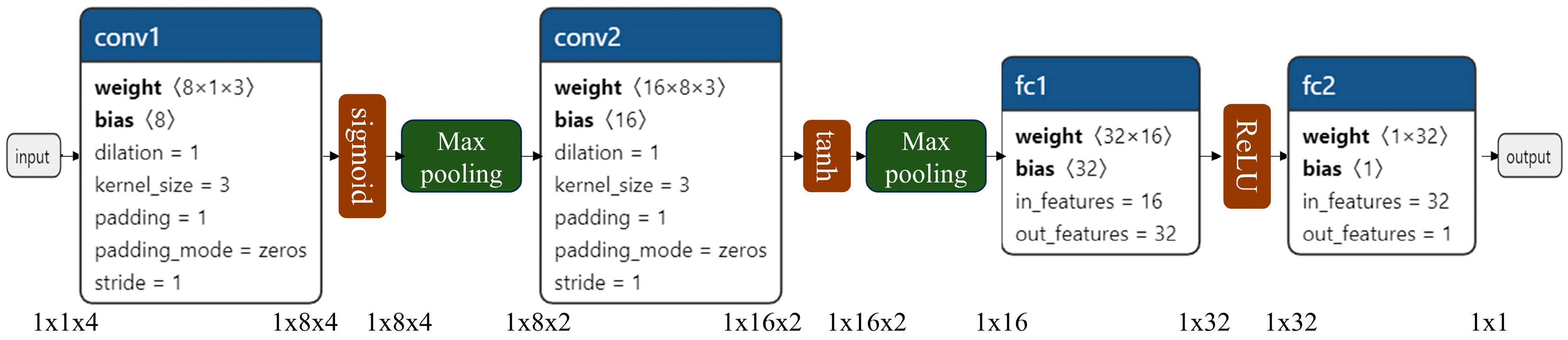
Figure 2.
Activation functions are used in the model.
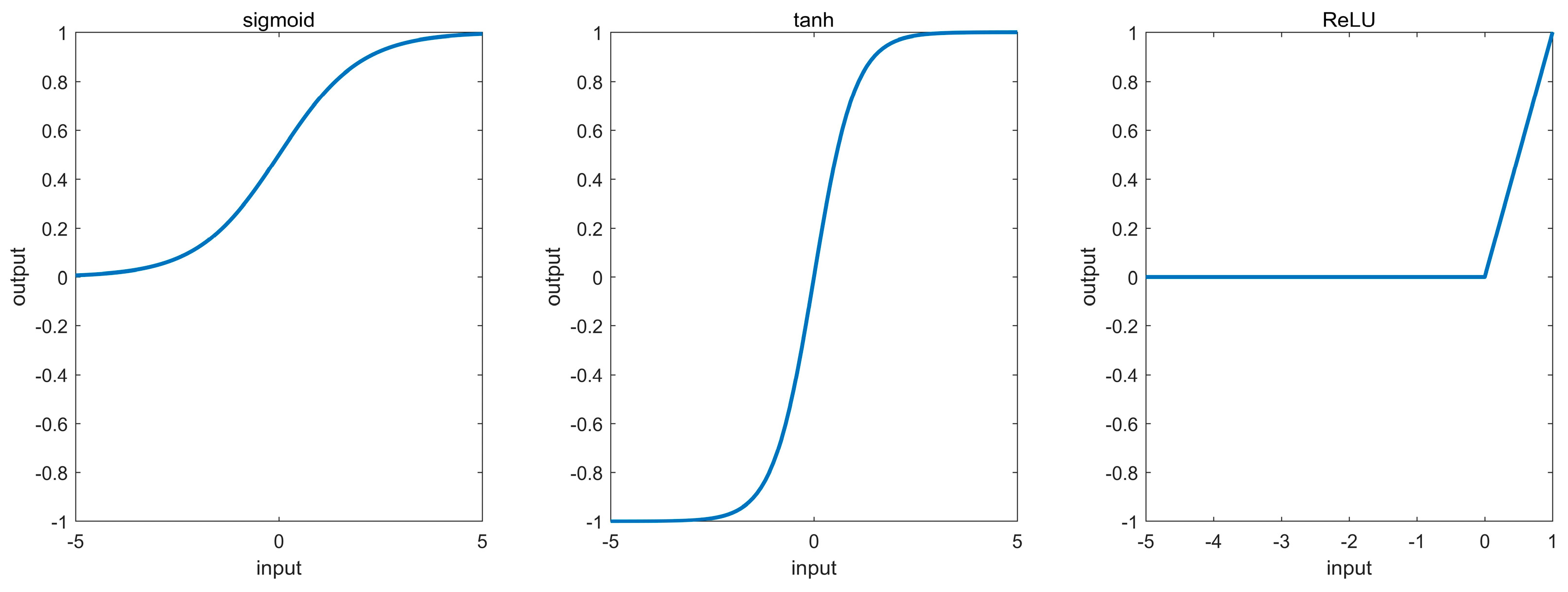
Figure 3.
Error distribution of the test set. (a) MAE; (b) RMSE; (c) MAXE.

Figure 4.
Error curves of the test set. (a) Error of depth; (b) Error of month.
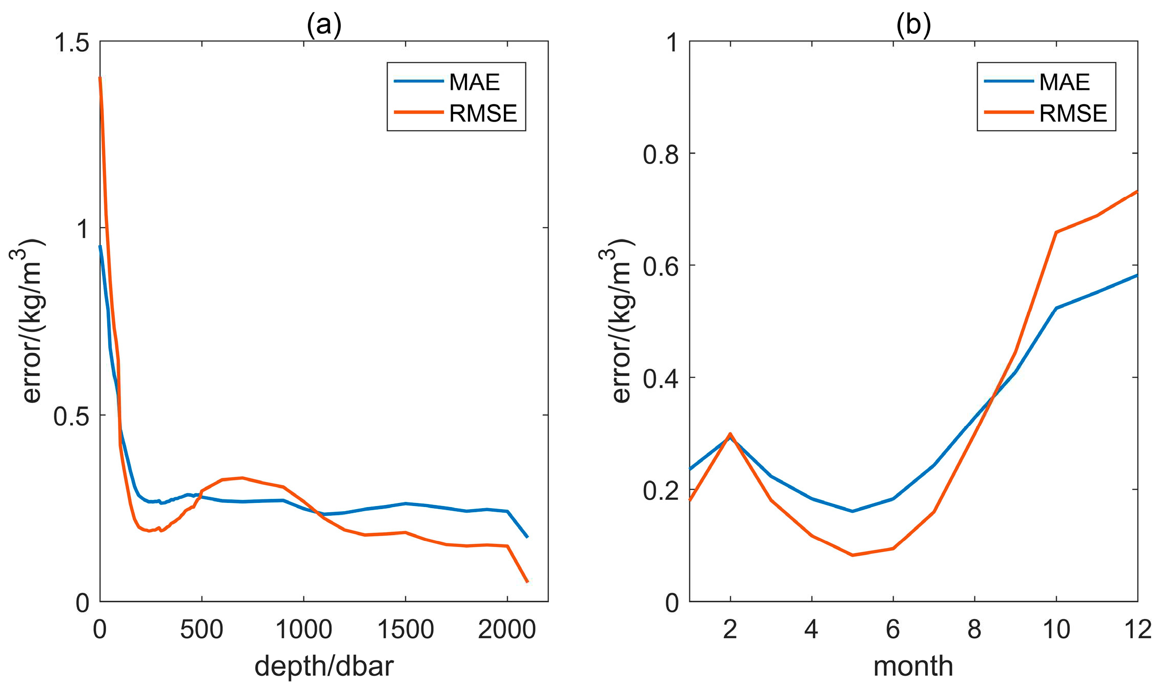
Figure 5.
The density of seawater output by the model varies with depth. The legend indicates that the letters "A", "I", and "P" correspond to the Atlantic, Indian, and Pacific Oceans, respectively. The month is December.
Figure 5.
The density of seawater output by the model varies with depth. The legend indicates that the letters "A", "I", and "P" correspond to the Atlantic, Indian, and Pacific Oceans, respectively. The month is December.
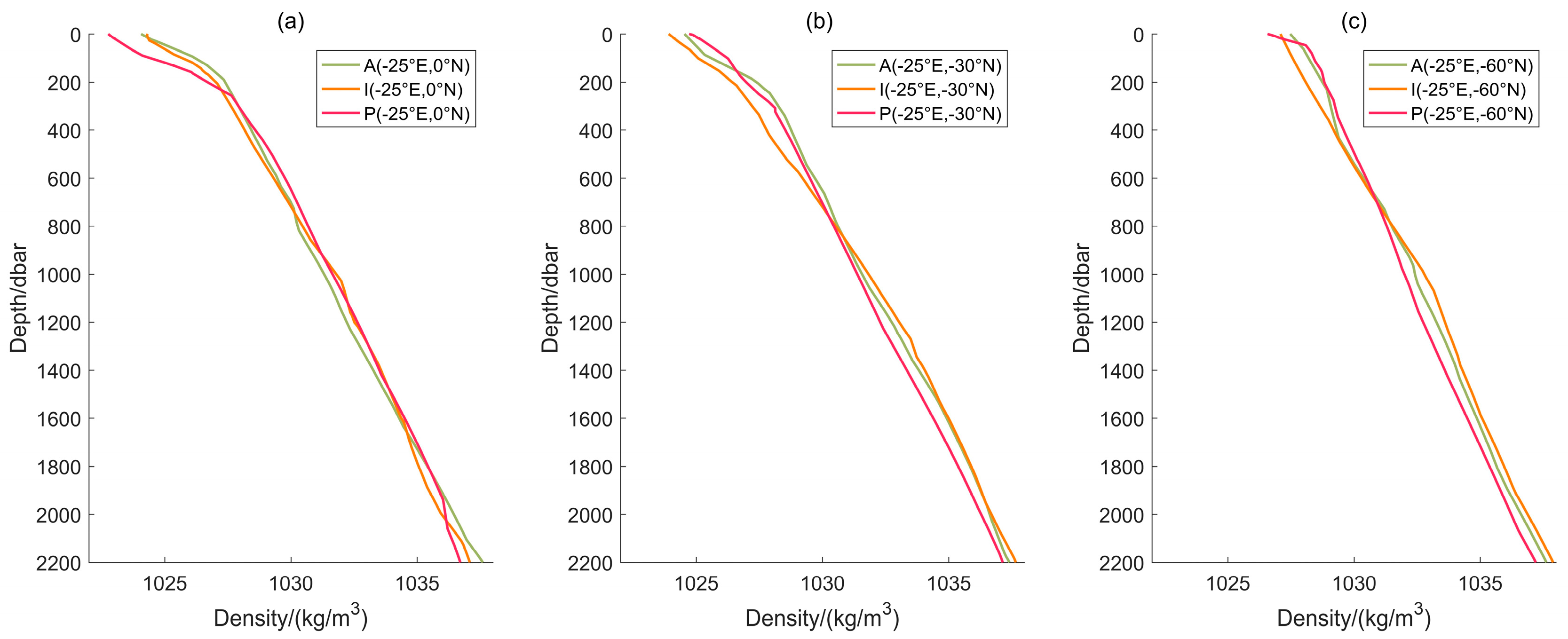
Figure 6.
Annual mean sea water density distribution at different depths. “Annual” refers to the average of the results of the model calculations from January to December.
Figure 6.
Annual mean sea water density distribution at different depths. “Annual” refers to the average of the results of the model calculations from January to December.
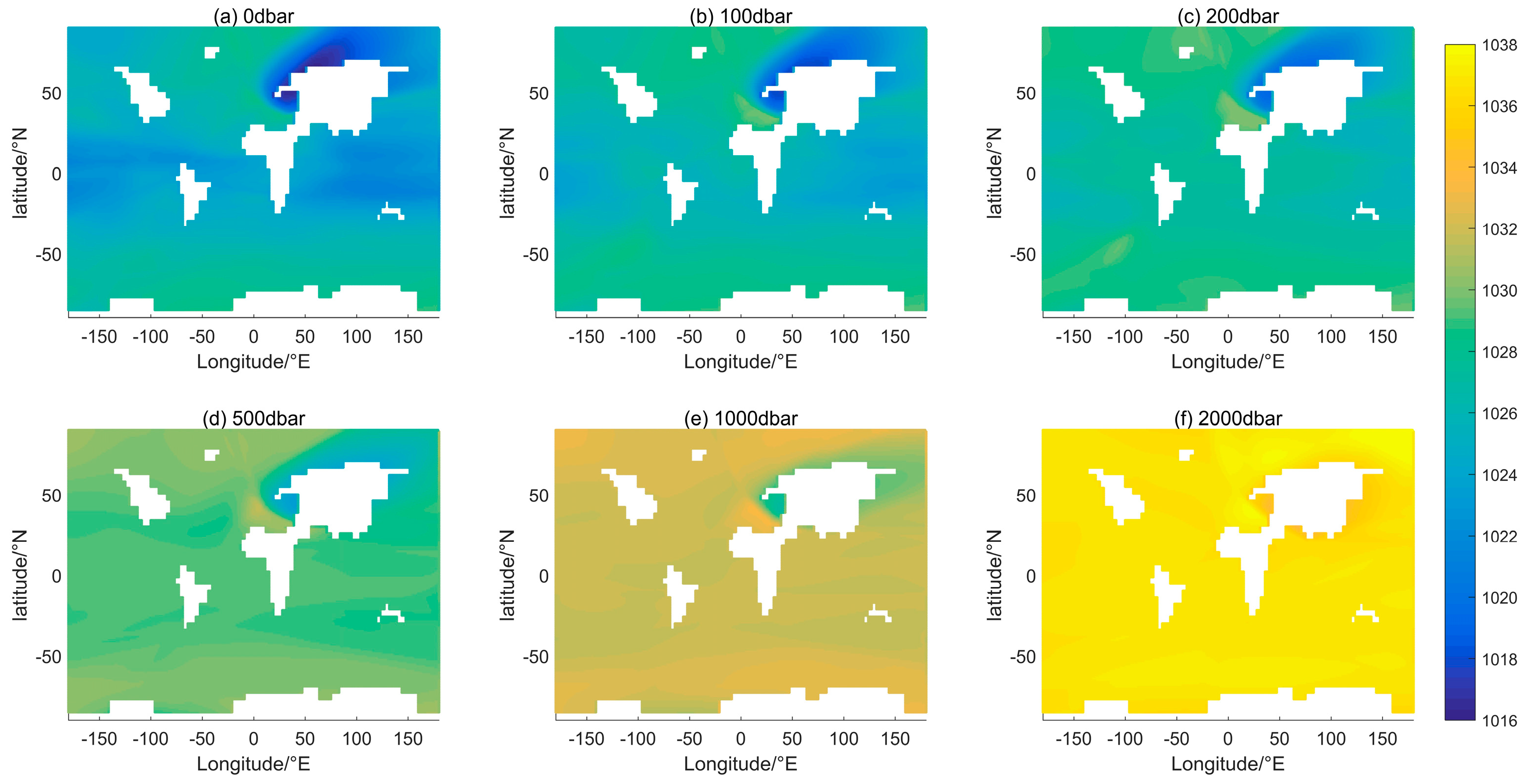
Figure 7.
Monthly mean surface density distribution in different seasons.
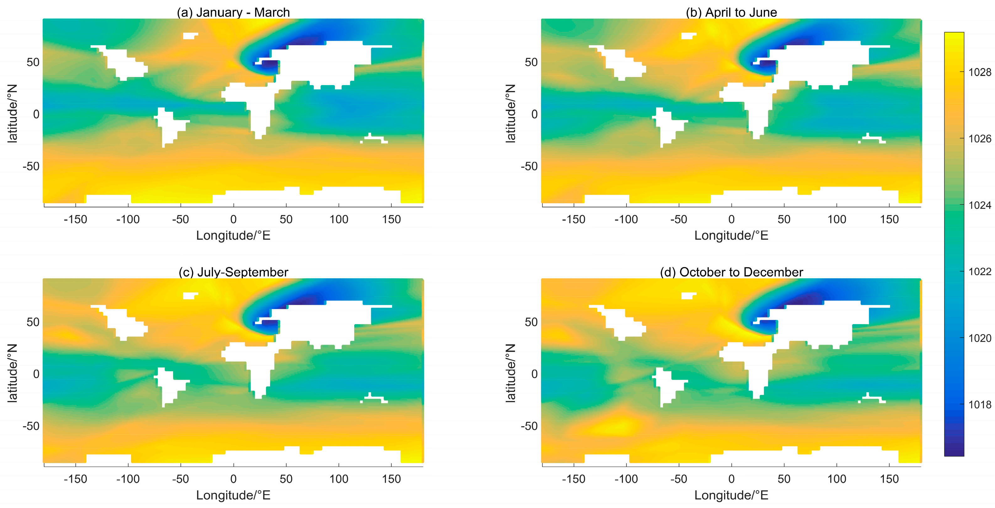

Table 1.
Input specifications for seawater density model.
| Input | Accuracy | Range |
|---|---|---|
| Latitude | 1° | -90 – 90 °N |
| Longitude | 1° | -180 – 180 °E |
| Depth | 0.01dbar | 0-2200 dbar |
| Month | 1 | 1-12 |
Disclaimer/Publisher’s Note: The statements, opinions and data contained in all publications are solely those of the individual author(s) and contributor(s) and not of MDPI and/or the editor(s). MDPI and/or the editor(s) disclaim responsibility for any injury to people or property resulting from any ideas, methods, instructions or products referred to in the content. |
© 2024 by the authors. Licensee MDPI, Basel, Switzerland. This article is an open access article distributed under the terms and conditions of the Creative Commons Attribution (CC BY) license (http://creativecommons.org/licenses/by/4.0/).
Copyright: This open access article is published under a Creative Commons CC BY 4.0 license, which permit the free download, distribution, and reuse, provided that the author and preprint are cited in any reuse.


