
Submitted:
04 January 2024
Posted:
05 January 2024
You are already at the latest version
Abstract
Convolutional neural networks (CNNs) have proven to be a very efficient class of machine learning (ML) architectures for handling multidimensional data by maintaining data locality, especially in the field of computer vision. Data pooling, a major component of CNNs, plays a crucial role for extracting important features of the input data and downsampling its dimensionality. Multidimensional pooling, however, is not efficiently implemented in existing ML algorithms. In particular, quantum machine learning (QML) algorithms have a tendency to ignore data locality for higher dimensions by representing/flattening multidimensional data as simple one-dimensional data. In this work, we propose using the quantum Haar transform (QHT) and quantum partial measurement for performing generalized pooling operations on multidimensional data. We present the corresponding decoherence-optimized quantum circuits for the proposed techniques along with their theoretical circuit depth analysis. Our experimental work was conducted using multidimensional data, ranging from 1-D audio data, to 2-D image data, to 3-D hyperspectral data, to demonstrate the scalability of the proposed methods. In our experiments, we utilized both noisy and noise-free quantum simulations on a state-of-the-art quantum simulator from IBM Quantum. We also show the efficiency of our proposed techniques for multidimensional data by reporting the fidelity of results.
Keywords:
quantum computing
; convolutional neural networks
; quantum machine learning
; pooling layers
1. Introduction
For performing machine learning (ML) tasks on multidimensional data, convolutional neural networks (CNNs) often outperforms other techniques, such as multi-layer perceptrons (MLPs), with smaller model size, shorter training time, and higher accuracy [1,2]. One factor that contributes to the benefits of CNNs is the conservation of spatio-temporal data locality, allowing them to preserve only relevant data connections and remove extraneous ones [1,2]. CNNs are constructed using a sequence of convolution and pooling pairs followed by a fully-connected layer [1]. In the convolution layer, filters are applied to input data for specific applications and the pooling layers reduce the spatial dimensions in the generated feature maps [3]. The reduced spatial dimensions generated from the pooling layers reduce memory requirements, which is a major concern for resource-constrained devices [4,5].
The benefits associated with exploiting data locality using pooling, can be translated to other domains, in particular quantum machine learning (QML). Notably, most of the existing QML algorithms do not consider the multidimensionality or data locality of input datasets by converting them into flattened 1-D arrays [6,7]. Nevertheless, quantum computing has shown great potential to outperform traditional, classical computing for specific machine learning tasks [8]. By exploiting quantum parallelism, superposition and entanglement, quantum computers can accelerate certain computation tasks with exponential speedups. However, in the current era of noisy intermediate-scale quantum (NISQ) devices, the implementation of quantum algorithms is constrained by the number of quantum bits (qubits) and fidelity of quantum gates [9]. For contemporary QML techniques, this problem is addressed by a hybrid approach where only the highly parallel and computationally-intensive part of the algorithm is executed in quantum hardware and the remaining parts are executed using classical computers [10]. Such methods, known as variational quantum algorithms (VQAs), exploit a fixed quantum circuit structure with parameterized rotation gates, denoted as ansatz, whose parameters are optimized using classical backpropagation techniques such as gradient descent [10].
In this work, we propose two generalized techniques for efficient pooling operations in QML, namely, quantum Haar transform (QHT) for quantum average pooling and partial quantum measurements for 2-norm/Euclidean pooling.
We characterize their fidelity to the corresponding classical pooling operations using a state-of-the-art quantum simulator from IBM Quantum for a wide variety of real-world, high-resolution, multidimensional data.
The rest of the paper is organized as follows. Section 2 covers necessary background information, including various quantum operations. Section 3 discusses existing related work. Section 4 introduces our proposed methodology, with great detail given to the constituent parts along with spatial complexity (depth) analysis of the corresponding circuits. Section 5 presents our experimental results, with an explanation of our verification metrics. Finally, Section 6 concludes our work and projects potential future directions.
2. Background
In this section, we provide information about quantum computing (QC) that is essential for understanding the proposed quantum pooling techniques.
2.1. Quantum Bits and States
2.2. Quantum Gates
Operations on qubits are called quantum gates and can be represented mathematically by unitary matrix operations. Serial and parallel composite operations can be constructed using matrix multiplications and tensor products, respectively [11,12]. In this section, we will present a number of relevant single- and multi-qubit gates for the proposed quantum pooling techniques.
2.2.1. Hadamard Gate
The Hadamard gate is a single-qubit gate that puts a qubit into superposition, see (3) [11].
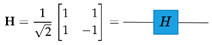
Parallel quantum operations acting on a different set of qubits can be combined using the tensor product [12]. For example, parallel single-qubit Hadamard gates can be represented by a unitary matrix, where each term in the resultant matrix can be directly calculated using the Walsh function [13], see (4).
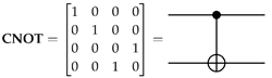
2.2.2. Controlled-NOT (CNOT) Gate
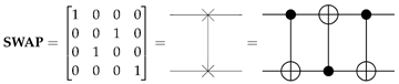
2.2.3. SWAP Gate
2.2.4. Quantum Perfect Shuffle Permutation (PSP)
The quantum perfect shuffle permutation (PSP) are operations that leverage SWAP gates to perform a cyclical rotation of the input qubits. The quantum PSP rotate-left (RoL) and rotate-right (RoR) operations [15] are shown in Figure 1. Each PSP operation requires SWAP operations or equivalently CNOT operations, see (6) and Figure 1.
2.2.5. Quantum Measurement
Although colloquially denoted as a measurement “gate”, the measurement or observation of a qubit is an irreversible non-unitary operation that projects a qubit’s quantum state to one of its or basis states [11]. The probability of either basis state being measured is directly determined by the square of the magnitude of each corresponding basis state coefficient, i.e., , and , see (7) [15].
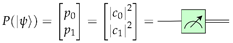
In general, an n-qubit quantum state has possible basis states/measurement outcomes. Accordingly, given full-measurement of a quantum statevector, the probability of finding the qubits in any particular state , where , is given by [15]. The overall probability distribution can thus be expressed according to (8).
3. Related Work
convolutional neural networks (CNNs) [16] represent a specialized type of neural network that consist of convolutional layers, pooling layers, and fully connected layers. The convolutional layer extracts characteristic features from an image, while the pooling layer down-scales the extracted features to a smaller data size by considering specific segments of data, often referred to as “windows” [1,16]. Pooling also enhances the network’s robustness to input translations and helps prevent overfitting [1]. For classical implementations on GPUs, pooling is usually limited to 3-D data [17,18], with a time complexity of [19], where N is the data size.
Quantum convolutional neural networks (QCNNs), as proposed by [7], explored the feasibility of extending the primary features and structures of conventional CNNs to quantum computers. However, translating the entire CNN model onto the presently available noisy intermediate-scale quantum (NISQ) devices is not practical due to limited qubit count [20], low decoherence time [21], and high gate errors [22]. To attain quantum advantage amid the constraints of NISQ devices, it is essential to develop depth-optimized convolution and pooling circuits that generate high fidelity outputs. Most implementations of quantum pooling [6,9,23,24,25] leverage parameterized quantum circuits (PQCs) and mid-circuit measurement as originally proposed in [7]. These techniques, however, do not perform the classical pooling operation as used in CNNs and thus do not gain the associated benefits from exploiting data locality. Moreover, PQC-based implementations of pooling increase the number of training parameters, which makes the classical optimization step more computationally intensive. The authors in [26] implemented quantum pooling by omitting measurement gates on a subset of qubits. However, the authors do not generalize their technique for varying window sizes, levels of decomposition, or data dimensions.
In this work, we propose a quantum average pooling technique based on the quantum Haar transform (QHT) [22] and a quantum Euclidean pooling technique utilizing partial measurement of quantum circuits. These techniques are generalizable for arbitrary window size and arbitrary data dimension. We have also provided the generalizable circuits for both techniques. The proposed methods have been validated with respect to their classical-implementation counterparts and their quality of results has been demonstrated by reporting the metric of quantum fidelity.
4. Materials and Methods
In this section, we discuss the proposed quantum pooling methods. Pooling, or downsampling, is a critical component of CNNs that consolidates similar features into one [2]. The most commonly used pooling schemes are average and maximum (max) pooling [27], where the two differ in terms of the sharpness of the defined input features. Max pooling typically offers a sharper definition of input features while average pooling offers a smoother definition of input features [27]. Depending on the desired application or dataset, one pooling technique may be preferable over the other [27].
Average and max pooling can be represented as special cases of calculating the p-norm or norm [28], where the p-norm of a vector of size N elements is given by (9a) for [28]. More specifically, average and max pooling can be defined as the 1-norm and ∞-norm, respectively, see (9b) and (9c). Since max pooling () is difficult to implement as a quantum (unitary) operation, a pooling scheme defined by the p-norm where could establish a balance between the average and max pooling schemes. Therefore, we introduce an intermediate pooling technique based on the 2-norm/Euclidean norm named as the quantum Euclidean pooling technique, see (9d).
In this work, we propose quantum pooling techniques for average pooling () and Euclidean pooling (). We implement average pooling using the QHT, a highly-parallelizable quantum algorithm for performing multilevel decomposition/reduction of multidimensional data. For the implementation of Euclidean pooling, we employ partial measurement to perform dimension reduction with zero circuit depth. The average and Euclidean pooling techniques are described in greater detail in Section 4.1 and Section 4.2, respectively. As detailed further in Section 5, we validated our proposed quantum pooling techniques using 1-D audio data [29], 2-D black-and-white (B/W) images [30], 3-D color (RGB) images [30], and 3-D hyperspectral images [31].
4.1. Quantum Average Pooling via Quantum Haar Transform
Our first proposed quantum pooling technique implements average pooling on quantum devices using the quantum wavelet transform (QWT). A wavelet transform decomposes the input data into low- and high-frequency components, where in the case of pooling, the low-frequency components represent the desired downsampled data [15]. For our proposed technique, we leverage the quantum variant of the first and simplest wavelet transform, quantum Haar transform (QHT) [15]. The execution of the pooling operation using QHT involves two main steps:
- Haar Wavelet Operation: By applying Hadamard (H) gates, see Section 2.2.1, in parallel, the high- and low-frequency components are decomposed from the input data.
- Data Rearrangement: By applying quantum rotate-right (RoR) operations, see Section 2.2.4, the high- and low-frequency components are grouped into contiguous regions.
We outline (in order) the following sections as follows, the quantum circuits and corresponding circuit depths of single-level decomposition, 1-D QHT, ℓ-level 1-D QHT, and ℓ-level d-D QHT, respectively, where ℓ is the number of decomposition levels and d is the dimensionality of the QHT operation.
4.1.1. Single-Level, One-Dimensional Quantum Haar Transform
For single-level, one-dimensional (1-D) QHT, we will assume a 1-D input data of size N data points. The aforementioned data would be encoded into the quantum circuit using amplitude encoding [32] as an n-qubit quantum state , where .
The quantum circuit for one level of 1-D QHT decomposition is shown in Figure 2, where represents the quantum state after the wavelet operation and represents the quantum state after data rearrangement.
4.1.1.1. Haar Wavelet Operation on Single-level, One Dimensional Data
The Haar wavelet is performed using the H gate, see Figure 2. For example, a single level of 1-D QHT can be performed on a state as described by (2) by applying a single H gate to the least-significant qubit of , designated in Figure 2. This operation replaces the data value of the pairs with their sum and difference, as shown in (10). It is worth mentioning that sum terms represent the low-frequency terms and the difference terms represent the high-frequency terms for a single level of decomposition.
4.1.1.2. Data Rearrangement Operation
The data rearrangement operation congregates the low- or high-frequency fragmented terms after decomposition. For instance, the low- and high-frequency terms are segregated after wavelet decomposition as expressed in (10). The low- and high-frequency terms exist at the even indices and odd indices respectively. Ideally, the statevector is formed in a way such that the low-frequency terms should be merged into a contiguous half of the overall statevector , while the rest of the statevector consists of the high-frequency terms . This data rearrangement operation can be performed using the qubit rotation using a RoR operation, see Figure 2 and (11).
4.1.1.3. Circuit Depth
The depth of the single-level 1-D QHT operation can be considered in terms of 1 H gate and 1 perfect-shuffle (RoR) gate. An RoR gate can be decomposed into SWAP gates or controlled-NOT (CNOT) gates. Accordingly, the total circuit depth can be expressed in terms of the number of consecutive single-qubit and controlled-NOT (CNOT) gates as shown in (12).
In many common quantum computing libraries, including Qiskit [33], it is possible to leverage arbitrary mapping of quantum registers to classical registers [34] to perform data rearrangement during quantum-to-classical (Q2C) data decoding without increasing circuit depth. Accordingly, the circuit depth of the optimized single-level, 1-D QHT circuit can be expressed as shown in (13).
4.1.2. Multilevel, One-Dimensional Quantum Haar Transform
In this section, we discuss how multiple levels (ℓ) of decomposition can be applied to further reduce the final data size. Given the initial data is set up in the same manner as in the single-level variant, the final data size can be expressed as . The corresponding quantum circuit for Multilevel, 1-D QHT is shown in Figure 3.
4.1.2.1. Haar Wavelet Operation on Multilevel, One-Dimensional Data
To perform multiple levels of decomposition, additional Hadamard gates are applied on the ℓ least-significant qubits of , as shown in Figure 3. The multilevel 1-D wavelet operation divides into groups of terms and replaces them with the appropriately-decomposed values according to the Walsh function, see (14).
4.1.2.2. Data Rearrangement Operation
Multiple levels of 1-D decomposition can be implemented using ℓ serialized RoR operations, see (15) and Figure 3. However, parallelization of the data rearrangement operation across multiple levels of decomposition can be achieved by overlapping/interleaving the rotate-right (RoR) operations into SWAP gates and fundamental two-qubit gates.
4.1.2.3. Circuit Depth
The inherent parallelizability of the wavelet and data rearrangement steps of QHT can be used to reduce the circuit depth. In the wavelet step, all ℓ levels of decomposition can be performed by ℓ parallel Hadamard gates (). In the data rearrangement step, the decomposition and interleaving of rotate-right (RoR) operations can used to reduce the depth penalty incurred by multilevel decomposition to just 2 SWAP gates, or 6 CNOT gates, per decomposition level, see (16).
Additionally, if the deferral of data rearrangement is permitted, the circuit depth of multilevel 1-D QHT can be shown to be constant (requiring just 1 Hadamard gate of depth), see (17).
4.1.3. Multilevel, Multidimensional Quantum Haar Transform
For multidimensional QHT, we can assume the input data is d-dimensional, where each dimension has a data size of for a total data size of . We can denote the largest dimension of data as , where it is encoded by qubits. Similarly, the smallest dimension of data is denoted as and is encoded by qubits. Similar to the 1-D case, the data is encoded as an n-qubit quantum state , such that each dimension i of data requires qubits and decomposition levels. It is worth mentioning that the total number of required qubits qubits and the final size of each data dimension i is .
Based on the nature of the encoding scheme (amplitude encoding) and quantum circuit structures, the multidimensional QHT can be performed by parallel application of d 1-D QHT circuits. Thus, the transformation of each data dimension can be performed independently of the other data dimensions. More specifically, using a column-major vectorization of the multidimensional data, the dimension of data is represented by the contiguous region of qubits to . In other words, multidimensional d-D QHT can be performed by stackingd 1-D QHT circuits in parallel, each of which performing the transformation on the respective contiguous region / data dimension, as shown in Figure 4.
4.1.3.1. Haar Wavelet Operation on Multidimensional Data
4.1.3.2. Data Rearrangement Operation
4.1.3.3. Circuit Depth
Since multidimensional QHT can be parallelized across dimensions, the circuit depth is determined by the dimension with the largest total data size and number of decomposition levels, as shown in (20).
If data rearrangement can be performed in the classical post-processing of Q2C data decoding, as discussed in Section 4.1.1, the wavelet operation is completely parallelized for multilevel and multidimensional QHT, resulting in an optimal, constant circuit depth, see (21).
4.2. Quantum Euclidean Pooling using Partial Measurement
Our second proposed quantum pooling technique applies the 2-norm or Euclidean norm over a given window of data. We implement the proposed Euclidean pooling technique using partial quantum measurement, which can be expressed mathematically either using conditional probabilities or partial traces of the density matrix [12].
As expressed in (8), full measurement of an n-qubit quantum state has possible outcomes, one for each basis state, where the probability of each outcome can be derived from the corresponding statevector . A subset of m qubits would only have possible outcomes, where . Thus, the probability distribution of the partial measurement can be derived from the probability distribution of the full measurement using conditional probability, where each qubit of the unmeasured qubits could arbitrarily be in either a 0 or 1 state [15]. For example, if the least-significant qubit is excluded from the measurements of the quantum state , the partial probability distribution is derived as shown in (22).
Alternatively, the probability distribution of a partial measurement can be derived from the diagonal of the partial trace of the density matrix [12]. For example, can also be calculated using the partial trace as shown in (23).
4.2.1. Single-level, One-Dimensional Quantum Euclidean Pooling
For single-level, one-dimensional Euclidean pooling, we will assume the input data is 1-D with N data size in terms of the number of data points. The input data is encoded using amplitude encoding as an n-qubit quantum state , where .
After applying one level of 1-D Euclidean pooling to the quantum state , the resultant state can be expressed as shown in (24). As discussed previously, it is possible to extract this partial quantum state using partial measurement, as shown in (22) and (23). The corresponding quantum circuit for the single-level, 1-D Euclidean pooling operation is presented in Figure 5.
4.2.2. Multilevel, One-Dimensional Quantum Euclidean Pooling
In multilevel, 1-D decomposition, as shown in Figure 6, the Euclidean norm (2-norm) of is taken with a window of , where the number of decomposition levels is ℓ, see (25) and Figure 6.
The change in normalization for 1-D pooling can be generalized with the corresponding increase in window size for the Euclidean norm, to , as shown in (26).
4.2.3. Multilevel, Multidimensional Quantum Euclidean Pooling
The multilevel, d-dimensional quantum Euclidean pooling circuit is illustrated in Figure 7, where is the number of decomposition levels for dimension i and . Similar to the multilevel, multidimensional QHT circuit discussed in Section 4.1.3, parallelization can be also applied to Euclidean pooling across dimensions using a stacked quantum circuit.
5. Experimental Work
In this section, we discuss our experimental setup and results. Experiments were conducted using real-world, high-resolution data, using both the quantum average and Euclidean pooling techniques. Section 5.1 delves into further detail on the experimental setup while Section 5.2 analyzes the obtained results.
5.1. Experimental Setup
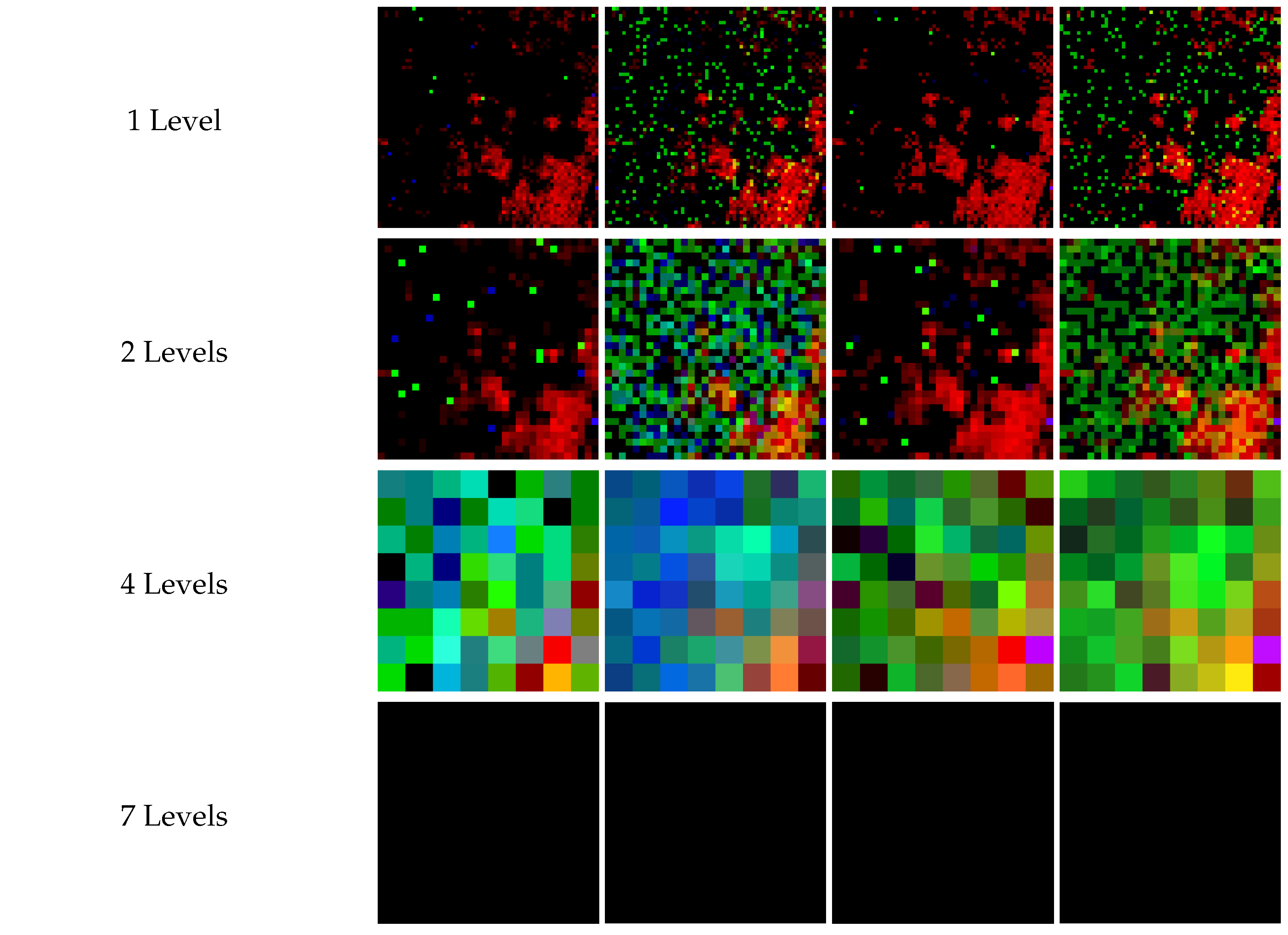
The efficacy of the two proposed pooling methods was examined through tests using real-world, high-resolution data of varying dimensions and data sizes. 1-D pooling was performed on selected publicly-available sound quality assessment material published by the European Broadcasting Union, which was pre-processed into a single channel with the data size ranging from data points to data points when sampled at kHz [29]. 2-D pooling was evaluated on black-and-white (B/W) and color (RGB) images of Jayhawks [30], as shown in Figure 8, sized from pixels to pixels. Additionally, 3-D pooling was performed on hyperspectral images from the Kennedy Space Center (KSC) dataset, see [31], were used, after pre-processing and resizing, with sizes ranging from () pixels to () pixels.
To validate the proposed pooling techniques, fidelity was measured over multiple levels of decomposition. The metric of data fidelity, see (27), is used to measure the similarity of the quantum-pooled data compared to the classically-pooled data . As expressed in during testing, pooling was performed on all tested dimensions until one dimension could not be decomposed further. For example, for a hyperspectral image of () pixels, ℓ was varied from 1 to , i.e., . Using the Qiskit SDK (v0.45.0) from IBM Quantum [33], simulations were run with the quantum average and Euclidean pooling circuits over the given data in both noise-free and noisy (with and circuit samples/shots) environments to display the effect of quantum statistical noise on the fidelity of the results. The experiments were performed at the University of Kansas on a computer cluster node populated with a 48-Core Intel Xeon Gold 6342 CPU, 3×NVIDIA A100 80GB GPUs (CUDA version 11.7), 256GB of 3200MHz DDR4 RAM, and PCIe 4.0 connectivity.
5.2. Results and Analysis
Across all our experiments, the noise-free quantum results showed 100% fidelity compared to the corresponding classical results, validating the correctness and theoretical soundness of our proposed quantum average and Euclidean pooling methods. However, for practical quantum environments, we observe measurement and statistical errors that are intrinsic to noisy quantum hardware, which results in a decrease in fidelity. Sample average and Euclidean pooling results are presented in Table 1, Table 2, Table 3, and Table 4 for 1-D Audio data, 2-D B/W images, 3-D RGB images, and 3-D Hyperspectral images, respectively, for noisy trials of and circuit samples (shots).
The presented results in Figure 9, Figure 10, Figure 11, Figure 12, Figure 13, Figure 14, Figure 15 and Figure 16 report the fidelity of the quantum-pooled data using our proposed quantum average and quantum Euclidean pooling techniques with respect to the corresponding classically-pooled data in terms of the data size indicated by the number of required qubits n for different levels of decomposition ℓ. 1-D audio data results are shown in Figure 9 and Figure 13 for and shots, respectively, while results for 2-D B/W images are shown in Figure 10 and Figure 14. In a similar fashion, results for 3-D RGB images are shown in Figure 11 and Figure 15, and finally results for 3-D hyperspectral data are shown in Figure 12 and Figure 16, all for and shots, respectively.
From Figure 9, Figure 10, Figure 11, Figure 12, Figure 13, Figure 14, Figure 15 and Figure 16, it could be easily observed that fidelity monotonically decreases with respect to data size (number of qubits) for a given decomposition level. In contrast, a monotonic increase in fidelity with respect to the number of decomposition levels for a given data size is observed, see Figure 9, Figure 10, Figure 11, Figure 12, Figure 13, Figure 14, Figure 15 and Figure 16. As the data size increases, the size of the corresponding quantum state also increases, which leads to statistical undersampling [15], a phenomenon that occurs when the number of measurement shots is insufficient to accurately characterize the measured quantum state. In quantum Euclidean pooling, partial measurement helps mitigate undersampling because the increase in decomposition levels reduces the number of qubits being measured, resulting in reduced effects of statistical undersampling/noise. A similar behavior occurs with quantum average pooling, since the high-frequency terms are sparse and/or close to 0. Nevertheless, quantum Euclidean pooling tends to achieve a slightly higher fidelity compared to quantum average pooling, see Figure 9, Figure 10, Figure 11, Figure 12, Figure 13, Figure 14, Figure 15 and Figure 16.
Table 5 compares the time complexity and generalizability of our proposed quantum pooling techniques to the existing classical and quantum pooling techniques. Compared to classical pooling techniques, our methods of average and Euclidean pooling can be performed in constant time for arbitrary data dimension and arbitrary pooling window size. The PQC-based techniques used in QCNNs [7], and its derivatives [6,9,23,24,25], are difficult to compare to other techniques since they don’t perform the same pooling operation. We can determine, however, that the additional ansatz for the PQC-based techniques would cause deeper quantum circuits compared to our proposed techniques. Finally, the measurement-based technique proposed in [26] is similar to our technique of single-level decomposition of 2-D Euclidean pooling (although their work inaccurately claims performing average pooling). However, our work is more generalizable for arbitrary windows sizes and data dimensions without compromising performance.
6. Conclusions
In this work, we proposed efficient quantum average and Euclidean pooling methods for multidimensional data that can be used in quantum machine learning (QML). Compared to existing classical and quantum techniques of pooling, our proposed techniques are highly generalizable for any dimensionality of data or levels of decomposition. Moreover, compared to the existing classical pooling techniques on GPUs, our proposed techniques can achieve significant speedup — from to for a data size of N values. We experimentally validated the correctness of our proposed quantum pooling techniques against the corresponding classical pooling techniques on 1-D audio data, 2-D image data, and 3-D hyperspectral data in a noise-free quantum simulator. We also presented results illustrating the effect on fidelity due to statistical and measurement errors using noisy quantum simulation. In future work, we will explore applications of the proposed pooling layers in QML algorithms.
Author Contributions
Conceptualization: M.J., V.J., D.K., and E.E.; Methodology: M.J., V.J., D.K., and E.E.; Software: M.J., D.L., D.K., and E.E.; Validation: M.J., V.J., D.L., A.N., D.K., and E.E.; Formal analysis: M.J., V.J., D.L., D.K., and E.E.; Investigation: M.J., A.N., V.J., D.L., D.K., M.C., I.I., E.B., E.V., A.F., M.S., A.A., and E.E.; Resources: M.J., A.N., V.J., D.L., D.K., M.C., I.I., E.B., E.V., A.F., M.S., A.A., and E.E.; Data curation: M.J., A.N., V.J., D.L., D.K., M.C., I.I., E.B., E.V., A.F., M.S., A.A., and E.E.; Writing—original draft preparation: M.J., A.N., V.J., D.L., D.K., M.C., I.I., and E.E.; Writing—review and editing: M.J., A.N., V.J., D.L., D.K., M.C., I.I., E.B., E.V., A.F., M.S., A.A., and E.E.; Visualization: M.J., A.N., V.J., D.L., D.K., M.C., I.I., E.B., E.V., A.F., M.S., A.A., and E.E.; Supervision: E.E.; Project administration: E.E.; Funding acquisition: E.E. All authors have read and agreed to the published version of the manuscript
Funding
This research received no external funding.
Data Availability Statement
The Jayhawk images used in this work are available on request from Brand Center, University of Kansas, at https://brand.ku.edu/ (last accessed on 12 December 2023) [30]. The audio samples used in this work are publicly available from the European Broadcasting Union at https://tech.ebu.ch/publications/sqamcd (accessed on 19 October 2023) as file 64.flac [29]. The hyperspectral data used in this work are publicly available from the Grupo de Inteligencia Computacional (GIC) at https://www.ehu.eus/ccwintco/index.php/Hyperspectral_Remote_Sensing_Scenes#Kennedy_Space_Center_(KSC) (accessed on 19 October 2023) under the heading Kennedy Space Center (KSC) [31].
Acknowledgments
This research used resources of the Oak Ridge Leadership Computing Facility, which is a DOE Office of Science User Facility supported under Contract DE-AC05-00OR22725.
Conflicts of Interest
The authors declare no conflicts of interest.
Abbreviations
The following abbreviations are used in this manuscript:
| 1-D | one-dimensional |
| 2-D | two-dimensional |
| 3-D | three-dimensional |
| B/W | black-and-white |
| CNN | convolutional neural network |
| CNOT | controlled-NOT |
| GPU | graphical processing unit |
| ML | machine learning |
| MLP | multi-layer perceptron |
| NISQ | noisy intermediate-scale quantum |
| PQC | parameterized quantum circuit |
| PSP | perfect shuffle permutation |
| Q2C | quantum-to-classical |
| QC | quantum computing |
| QCNN | quantum convolutional neural network |
| QHT | quantum Haar transform |
| QML | quantum machine learning |
| QWT | quantum wavelet transform |
| RGB | color |
| RoL | rotate-left |
| RoR | rotate-right |
| VQA | variational quantum algorithm |
References
- LeCun, Y.; Kavukcuoglu, K.; Farabet, C. Convolutional networks and applications in vision. In Proceedings of the Proceedings of 2010 IEEE international symposium on circuits and systems. IEEE. 2010; 253–256. [Google Scholar]
- LeCun, Y.; Bengio, Y.; Hinton, G. Deep learning. Nature 2015, 521, 436–444. [Google Scholar] [CrossRef] [PubMed]
- Gholamalinezhad, H.; Khosravi, H. Pooling methods in deep neural networks, a review. arXiv 2020, arXiv:2009.07485. [Google Scholar]
- Chen, F.; Datta, G.; Kundu, S.; Beerel, P.A. Self-Attentive Pooling for Efficient Deep Learning. In Proceedings of the Proceedings of the IEEE/CVF Winter Conference on Applications of Computer Vision. 2023; 3974–3983. [Google Scholar]
- Tabani, H.; Balasubramaniam, A.; Marzban, S.; Arani, E.; Zonooz, B. Improving the efficiency of transformers for resource-constrained devices. In Proceedings of the 2021 24th Euromicro Conference on Digital System Design (DSD). IEEE. 2021; 449–456. [Google Scholar]
- Hur, T.; Kim, L.; Park, D.K. Quantum convolutional neural network for classical data classification. Quantum Machine Intelligence 2022, 4, 3. [Google Scholar] [CrossRef]
- Cong, I.; Choi, S.; Lukin, M.D. Quantum convolutional neural networks. Nature Physics 2019, 15, 1273–1278. [Google Scholar] [CrossRef]
- Biamonte, J.; Wittek, P.; Pancotti, N.; Rebentrost, P.; Wiebe, N.; Lloyd, S. Quantum machine learning. Nature 2017, 549, 195–202. [Google Scholar] [CrossRef] [PubMed]
- Monnet, M.; Gebran, H.; Matic-Flierl, A.; Kiwit, F.; Schachtner, B.; Bentellis, A.; Lorenz, J.M. Pooling techniques in hybrid quantum-classical convolutional neural networks. arXiv 2023, arXiv:2305.05603. [Google Scholar]
- Peruzzo, A.; McClean, J.; Shadbolt, P.; Yung, M.H.; Zhou, X.Q.; Love, P.J.; Aspuru-Guzik, A.; O’Brien, J.L. A variational eigenvalue solver on a photonic quantum processor. Nature Communications 2014, 5, 4213. [Google Scholar] [CrossRef] [PubMed]
- Williams, C.P.; Clearwater, S.H. Explorations in quantum computing; Springer, 1998.
- Nielsen, M.A.; Chuang, I.L. Quantum Computation and Quantum Information: 10th Anniversary Edition; Cambridge University Press, 2010; pp. 5,13,15,17,65,71,105–107,374,409. [CrossRef]
- Walsh, J.L. A Closed Set of Normal Orthogonal Functions. American Journal of Mathematics 1923, 45, 5–24. [Google Scholar] [CrossRef]
- Shende, V.; Bullock, S.; Markov, I. Synthesis of quantum-logic circuits. IEEE Transactions on Computer-Aided Design of Integrated Circuits and Systems 2006, 25, 1000–1010. [Google Scholar] [CrossRef]
- Jeng, M.; Islam, S.I.U.; Levy, D.; Riachi, A.; Chaudhary, M.; Nobel, M.A.I.; Kneidel, D.; Jha, V.; Bauer, J.; Maurya, A.; et al. Improving quantum-to-classical data decoding using optimized quantum wavelet transform. The Journal of Supercomputing 2023. [Google Scholar] [CrossRef]
- LeCun, Y.; Bottou, L.; Bengio, Y.; Haffner, P. Gradient-based learning applied to document recognition. Proceedings of the IEEE 1998, 86, 2278–2324. [Google Scholar] [CrossRef]
- NVIDIA. cuDNN - cudnnPoolingForward() [computer software]. https://docs.nvidia.com/deeplearning/cudnn/api/index.html#cudnnPoolingForward, 2023. [Last accessed: 2023-12-30].
- NVIDIA. TensorRT - Pooling [computer software]. https://docs.nvidia.com/deeplearning/tensorrt/operators/docs/Pooling.html, 2023. [Last accessed: 2023-12-30].
- NVIDIA. Pooling. https://docs.nvidia.com/deeplearning/performance/dl-performance-memory-limited/index.html#pooling, 2023. [Last accessed: 2023-12-30].
- El-Araby, E.; Mahmud, N.; Jeng, M.J.; MacGillivray, A.; Chaudhary, M.; Nobel, M.A.I.; Islam, S.I.U.; Levy, D.; Kneidel, D.; Watson, M.R.; et al. Towards Complete and Scalable Emulation of Quantum Algorithms on High-Performance Reconfigurable Computers. IEEE Transactions on Computers 2023. [Google Scholar] [CrossRef]
- Schlosshauer, M. Quantum decoherence. Physics Reports 2019, 831, 1–57. [Google Scholar] [CrossRef]
- Mahmud, N.; MacGillivray, A.; Chaudhary, M.; El-Araby, E. Decoherence-optimized circuits for multidimensional and multilevel-decomposable quantum wavelet transform. IEEE Internet Computing 2021, 26, 15–25. [Google Scholar] [CrossRef]
- MacCormack, I.; Delaney, C.; Galda, A.; Aggarwal, N.; Narang, P. Branching quantum convolutional neural networks. Physical Review Research 2022, 4, 013117. [Google Scholar] [CrossRef]
- Chen, G.; Chen, Q.; Long, S.; Zhu, W.; Yuan, Z.; Wu, Y. Quantum convolutional neural network for image classification. Pattern Analysis and Applications 2023, 26, 655–667. [Google Scholar] [CrossRef]
- Zheng, J.; Gao, Q.; Lü, Y. Quantum graph convolutional neural networks. In Proceedings of the 2021 40th Chinese Control Conference (CCC). IEEE; 2021; pp. 6335–6340. [Google Scholar]
- Wei, S.; Chen, Y.; Zhou, Z.; Long, G. A quantum convolutional neural network on NISQ devices. AAPPS Bulletin 2022, 32, 1–11. [Google Scholar] [CrossRef]
- Bieder, F.; Sandkühler, R.; Cattin, P.C. Comparison of Methods Generalizing Max- and Average-Pooling. 2021; arXiv:cs.CV/2103.01746]. [Google Scholar]
- PyTorch. torch.nn.LPPool1d [computer software]. https://pytorch.org/docs/stable/generated/torch.nn.LPPool1d.html, 2023. [Last accessed: 2023-12-30].
- Geneva, S. Sound Quality Assessment Material: Recordings for Subjective Tests. https://tech.ebu.ch/publications/sqamcd, 1988. Last Accessed: 2023-10-19.
- Brand Center, University of Kansas. Jayhawk Images. https://brand.ku.edu/. Last Accessed: 2023-12-30.
- Graña, M. ; M.A., V.; B., A. Hyperspectral Remote Sensing Scenes. https://www.ehu.eus/ccwintco/index.php/Hyperspectral_Remote_Sensing_Scenes#Kennedy_Space_Center_(KSC). Last Accessed: 2023-10-19.
- El-Araby et al., E. Towards Complete and Scalable Emulation of Quantum Algorithms on High-Performance Reconfigurable Computers. IEEE Transactions on Computers 2023, 72, 2350–2364. [CrossRef]
- IBM Quantum. Qiskit: An Open-source Framework for Quantum Computing, 2021. [CrossRef]
- IBM Quantum. qiskit.circuit.QuantumCircuit.measure [computer software]. https://docs.quantum.ibm.com/api/qiskit/qiskit.circuit.QuantumCircuit#measure, 2023. [Last accessed: 2023-12-30].
Figure 1.
Rotate-Left and Rotate-Right operations.
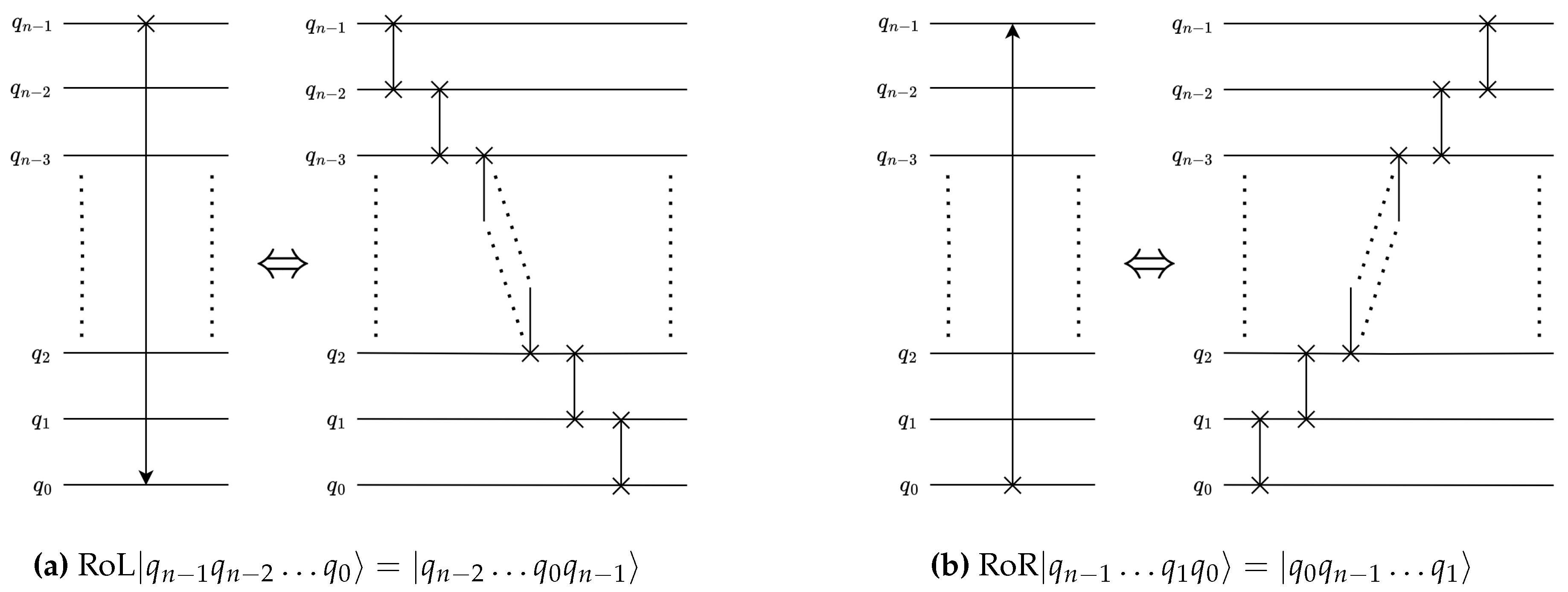
Figure 2.
Single-level, 1-D QHT circuit.
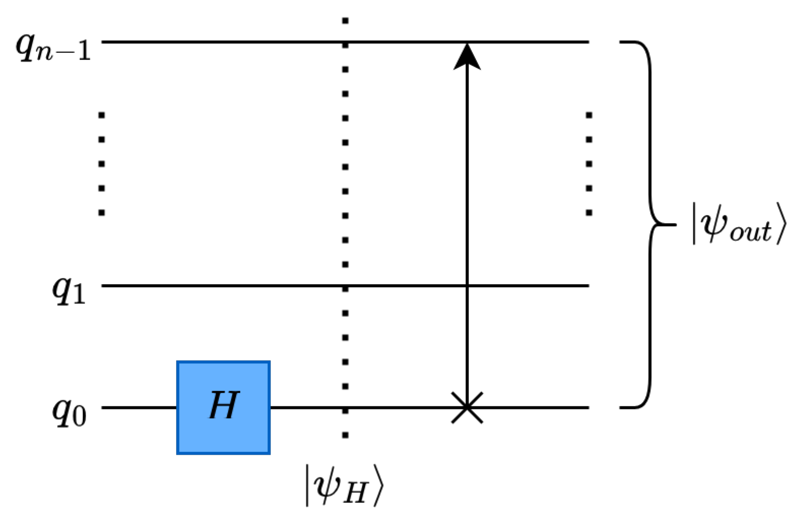
Figure 3.
Multilevel, 1-D QHT circuit.
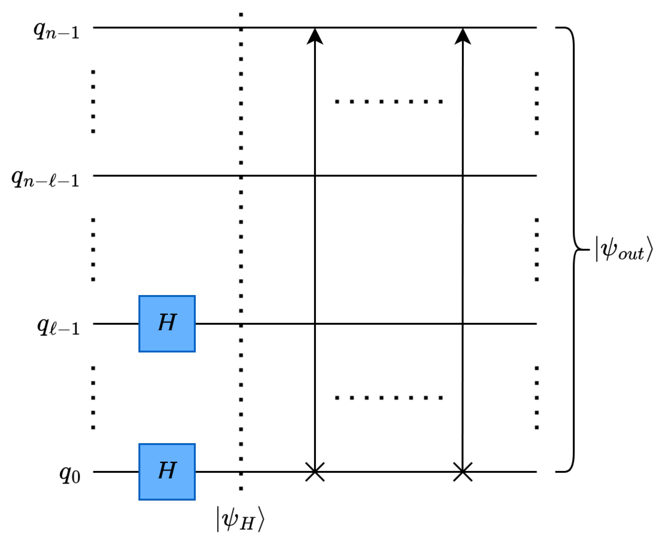
Figure 4.
Multilevel, d-D quantum Haar transform (QHT) circuit.
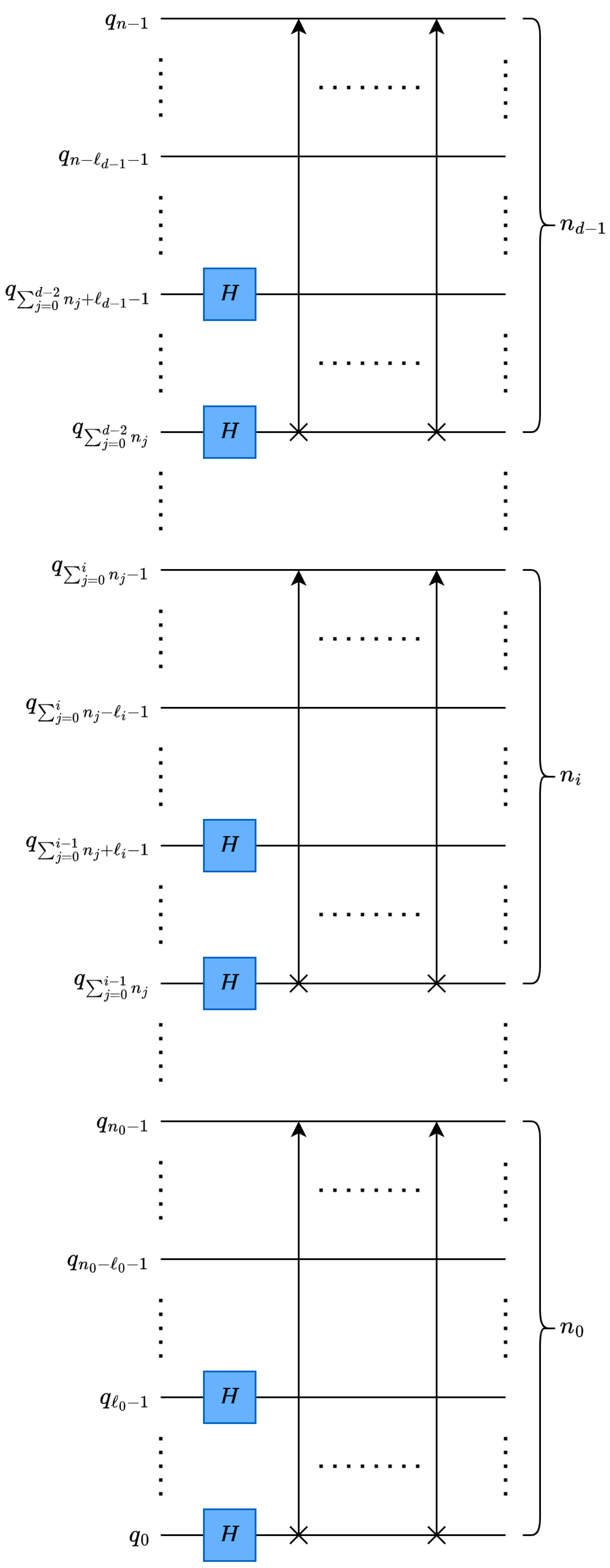
Figure 5.
Single-level, 1-D Euclidean pooling circuit.
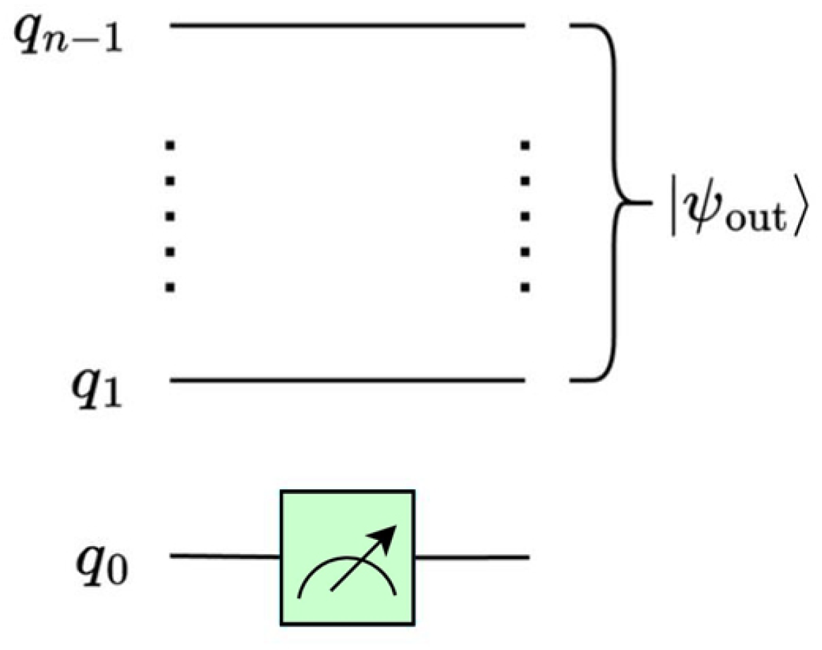
Figure 6.
Multilevel, 1-D Euclidean pooling circuit.
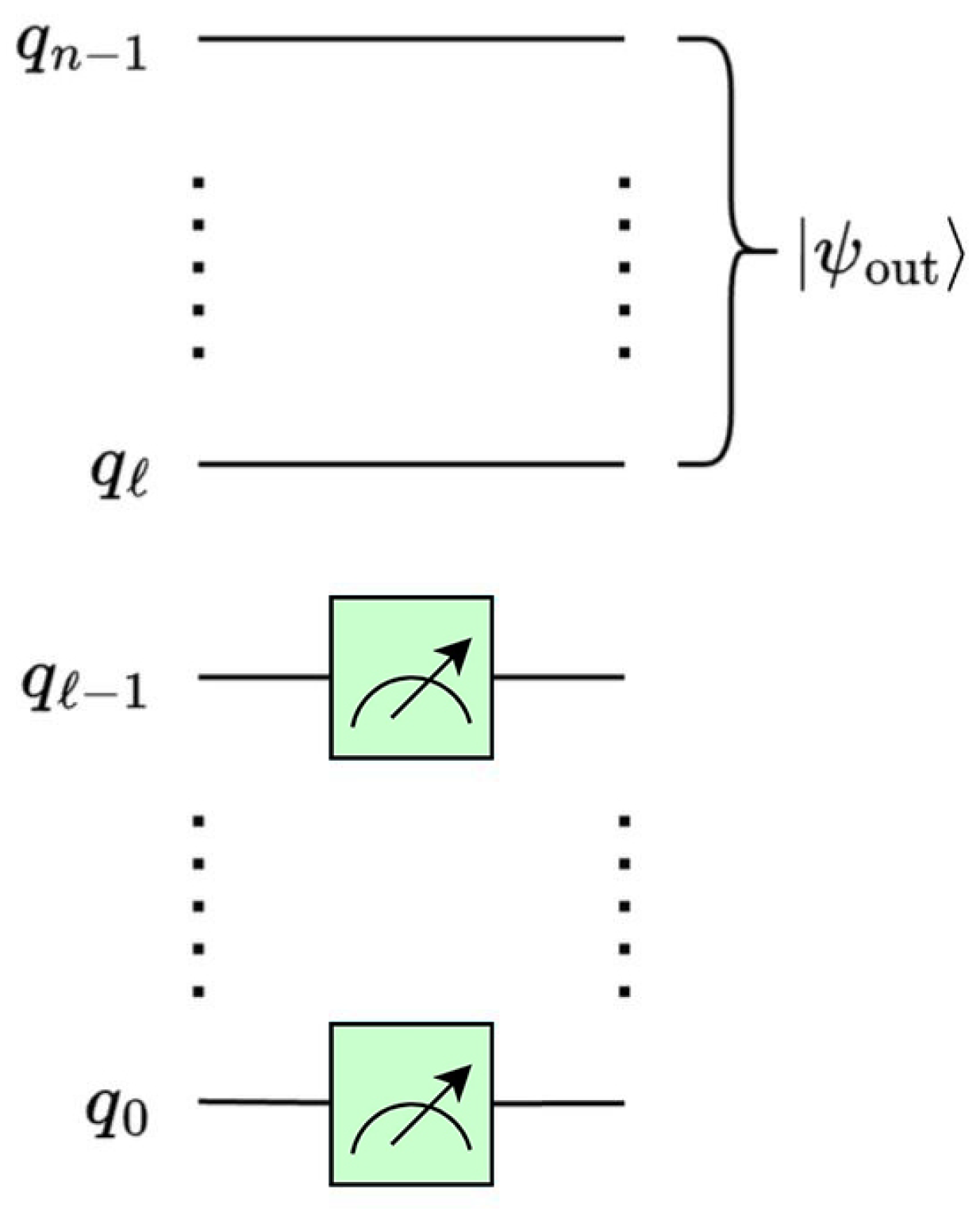
Figure 7.
Multilevel, d-D Euclidean pooling circuit.
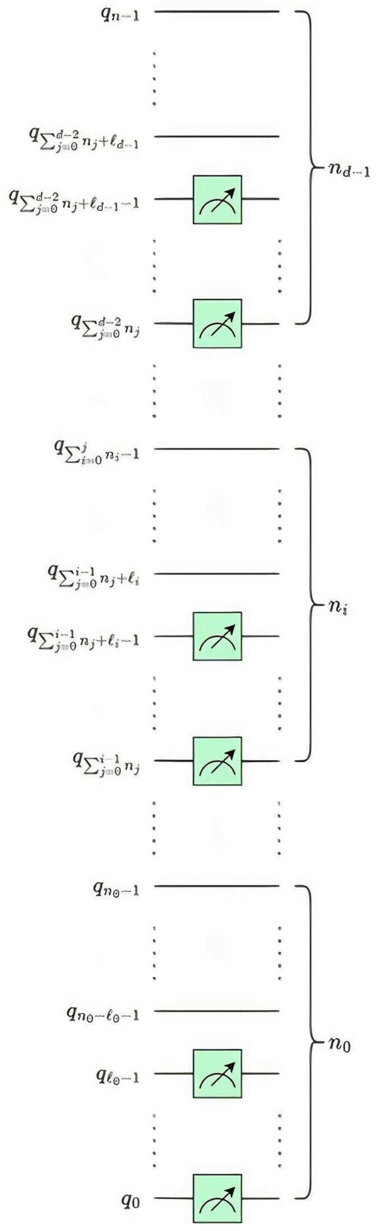
Figure 8.
Real-world, high-resolution, multidimensional data used in experimental trials. (a) B/W Image [30]. (b) RGB Image [30]. (c) Hyperspectral Image [31].
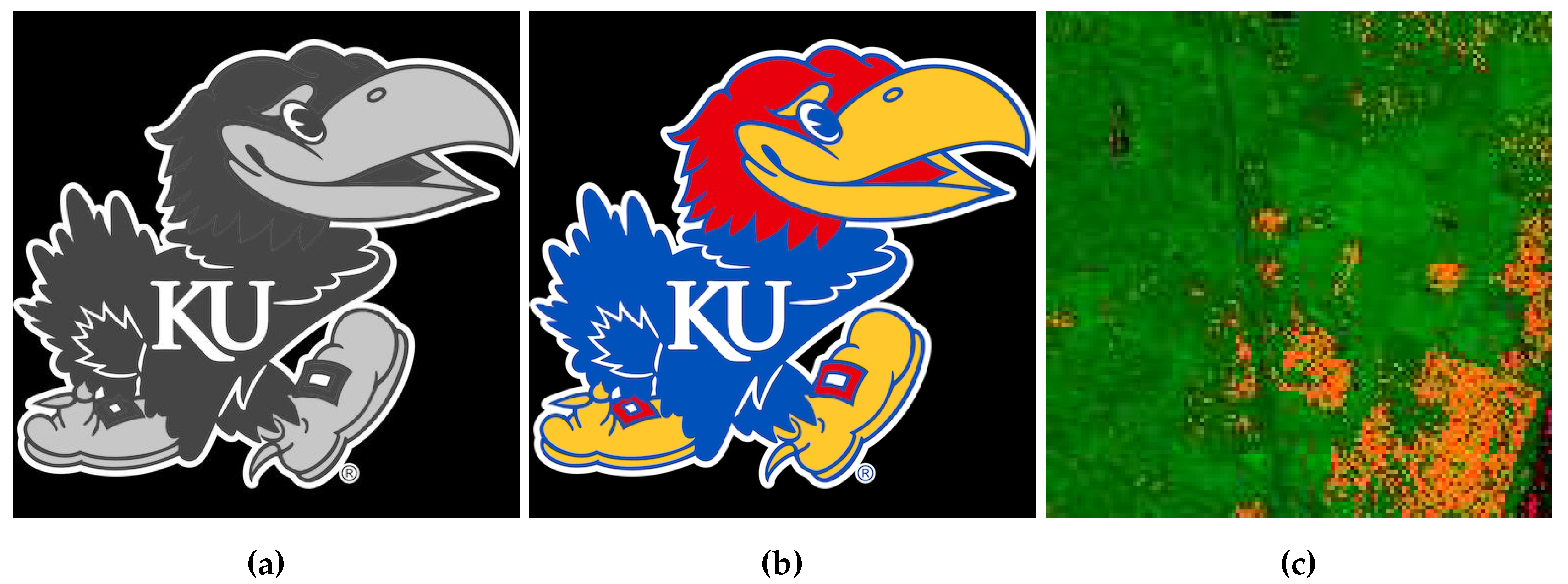
Figure 9.
Fidelity of 1-D Pooling on 1-D Audio data ( shots)
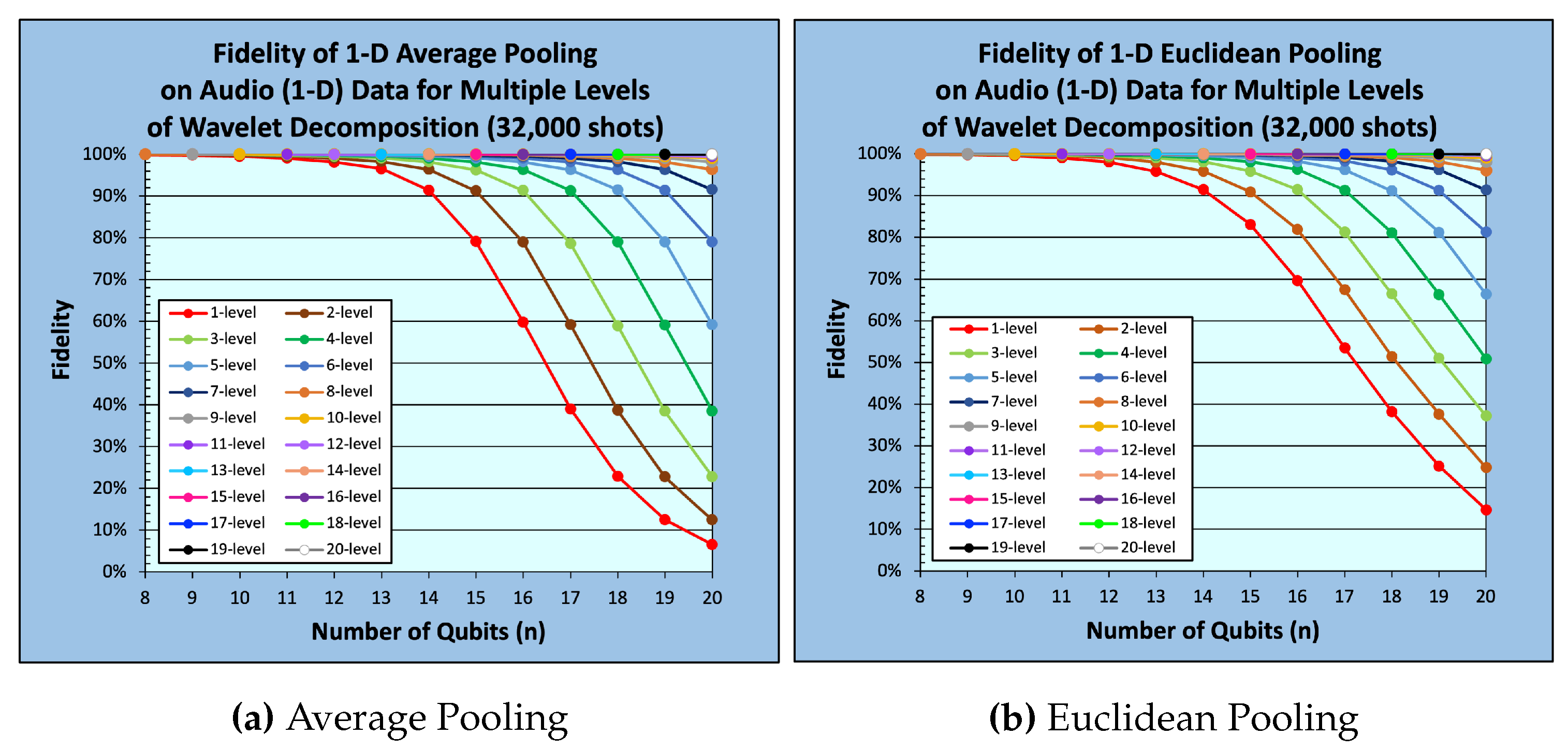
Figure 10.
Fidelity of 2-D Pooling on 2-D B/W Images ( shots)
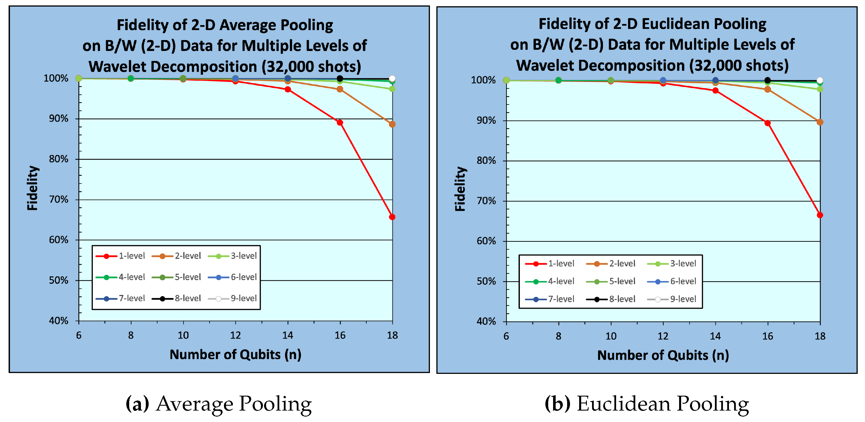
Figure 11.
Fidelity of 2-D Pooling on 3-D RGB Images ( shots)
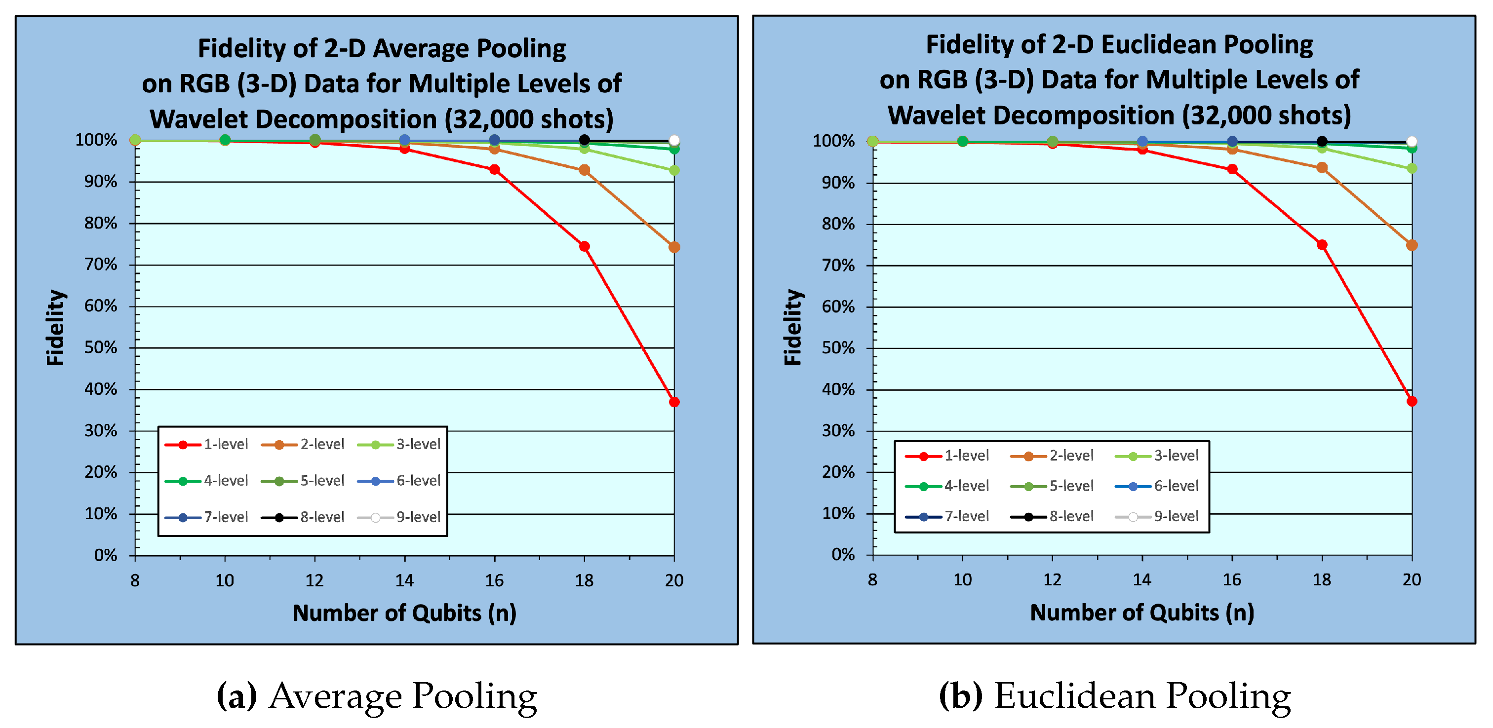
Figure 12.
Fidelity of 3-D Pooling on Hyperspectral Images ( shots)
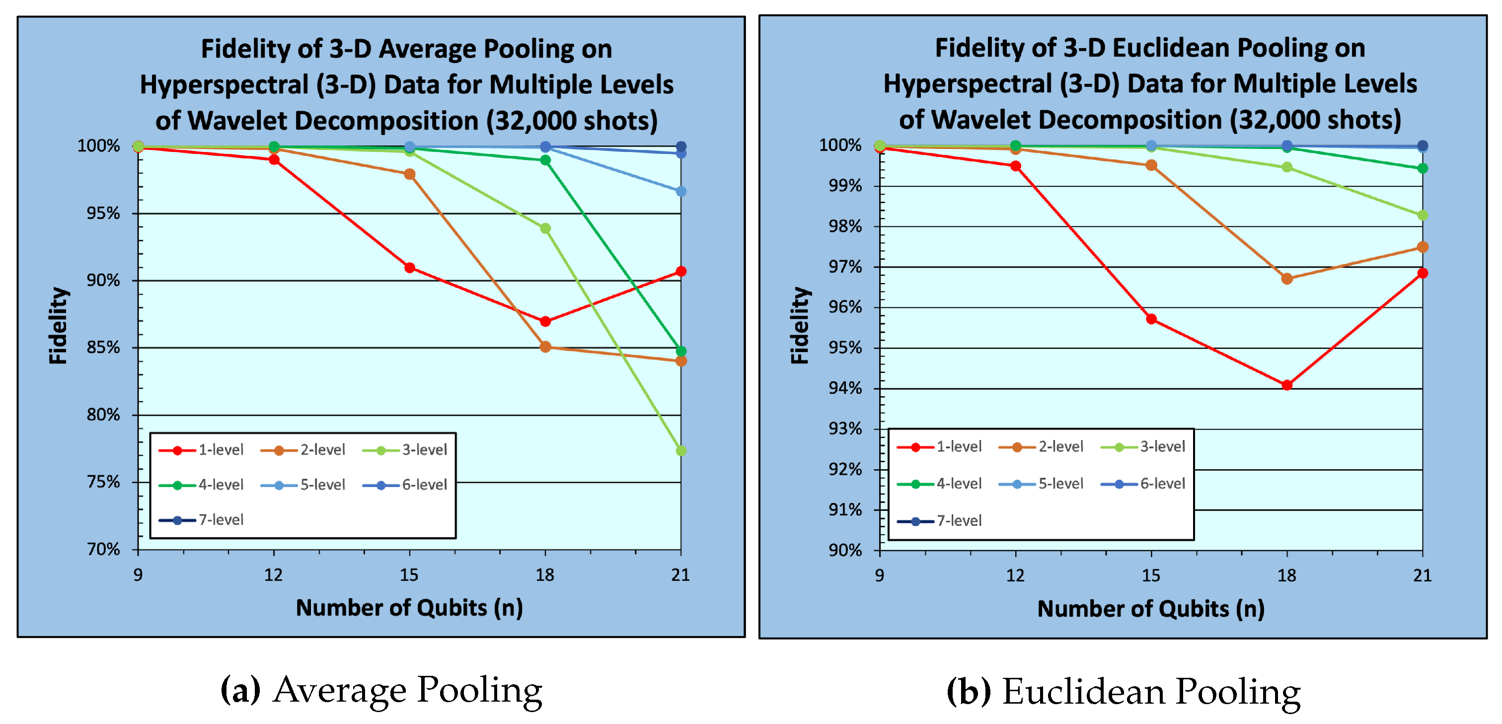
Figure 13.
Fidelity of 1-D Pooling on 1-D Audio data ( shots)
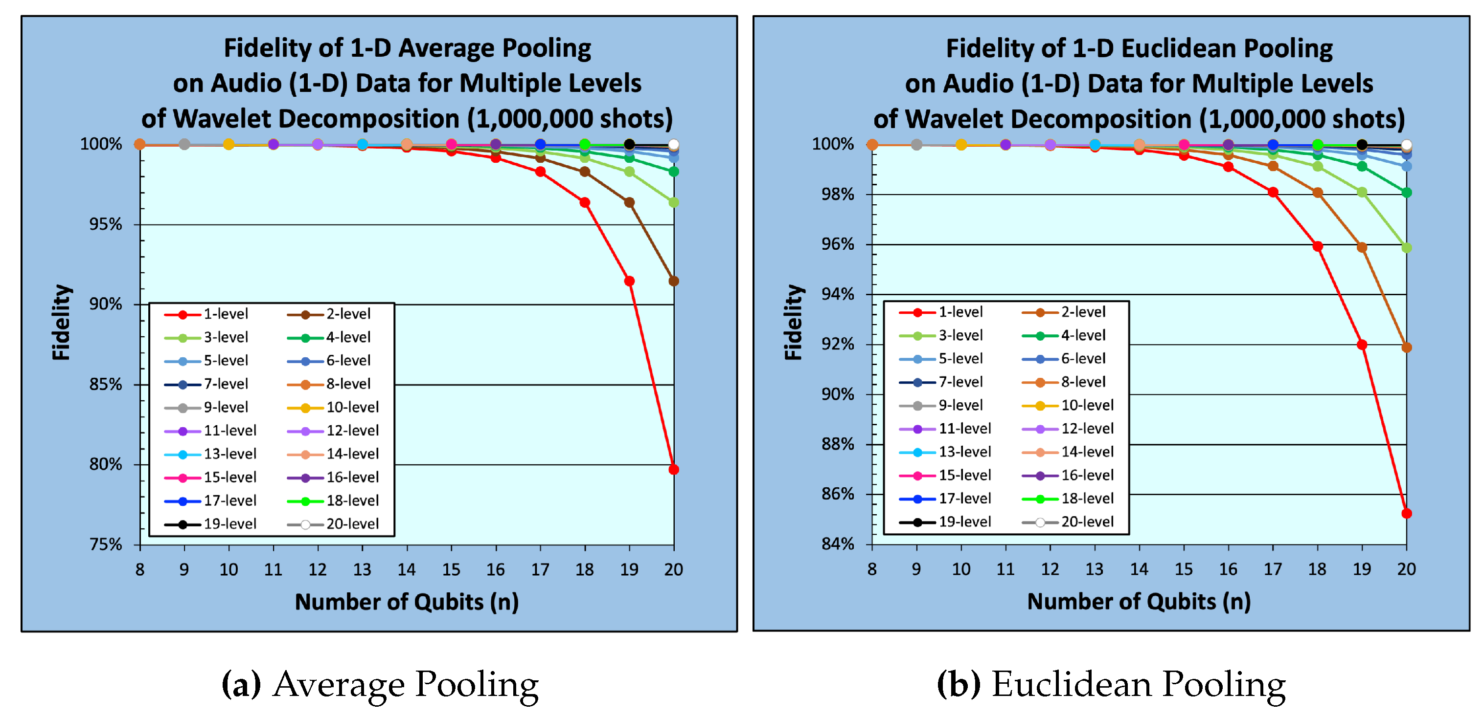
Figure 14.
Fidelity of 2-D Pooling on 2-D B/W Images ( shots)
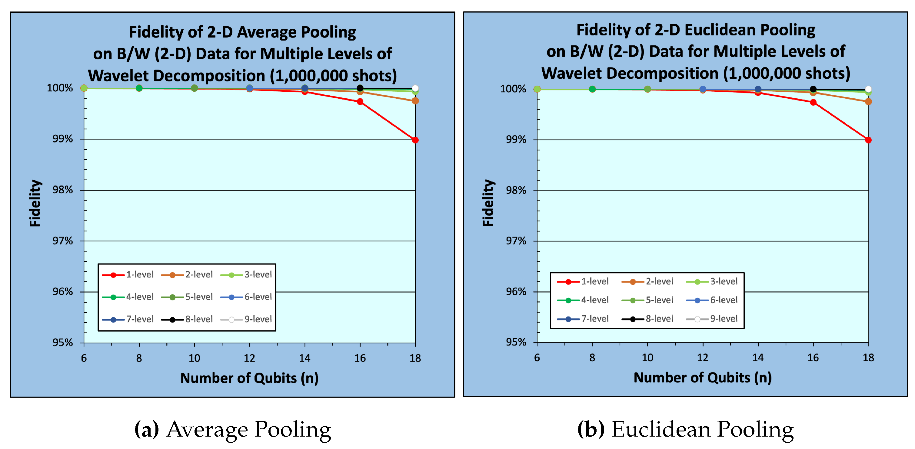
Figure 15.
Fidelity of 2-D Pooling on 3-D RGB Images ( shots)
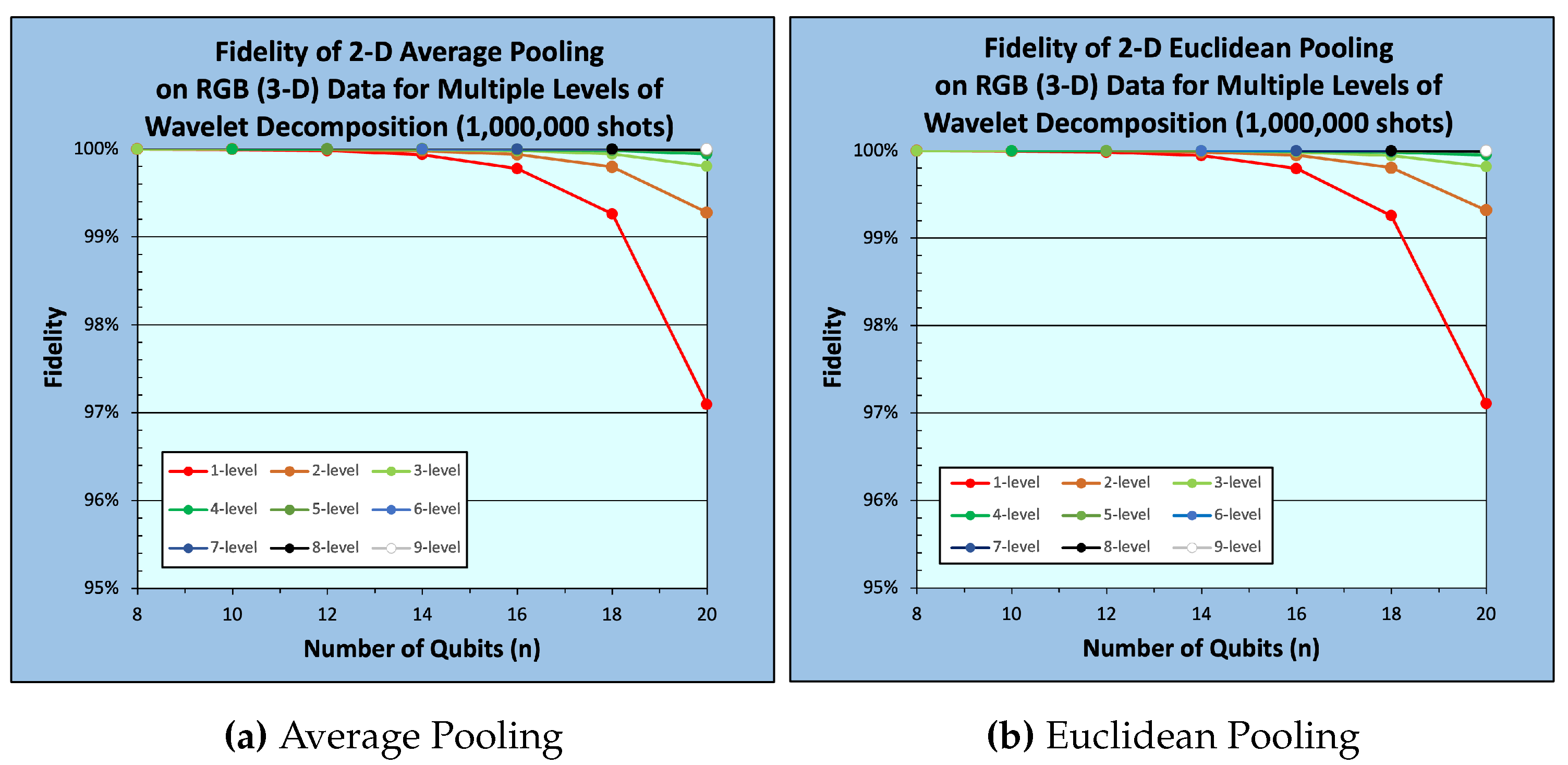
Figure 16.
Fidelity of 3-D Pooling on 3-D Hyperspectral Images ( shots)
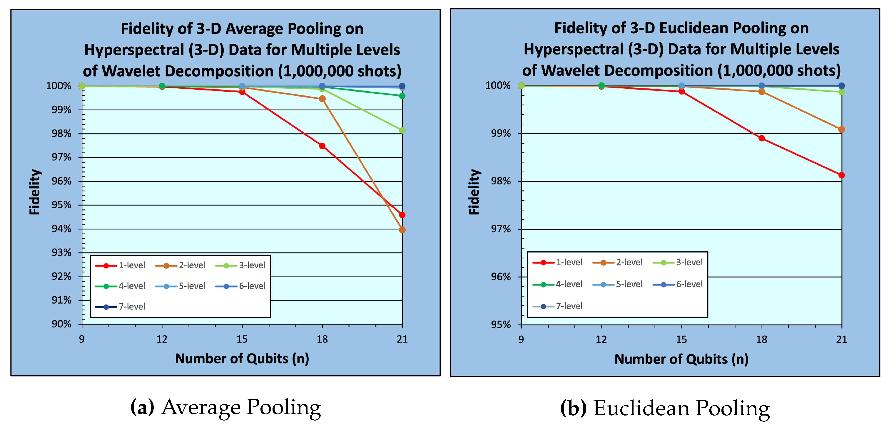

Table 1.
Noisy outputs for 1-D Average and Euclidean Pooling on Audio (1-D) data [29] with audio samples.
Table 1.
Noisy outputs for 1-D Average and Euclidean Pooling on Audio (1-D) data [29] with audio samples.
| Levels of Decomposition | Average Pooling ( shots) |
Average Pooling ( shots) |
Euclidean Pooling ( shots) |
Euclidean Pooling ( shots) |
|---|---|---|---|---|
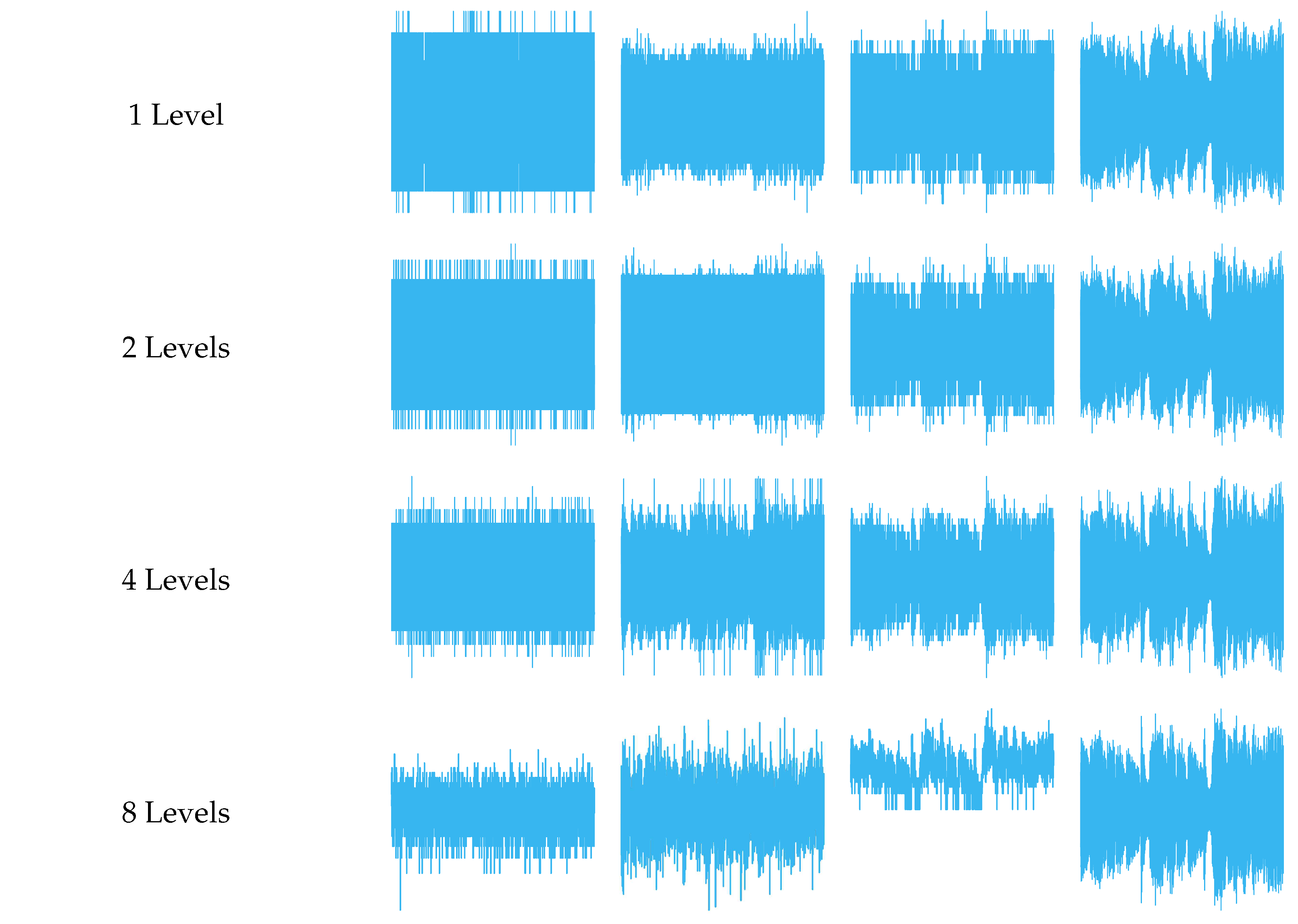 | ||||
Table 2.
Noisy outputs for 2-D Average and Euclidean Pooling on B/W (2-D) data of size () pixels.
| Levels of Decomposition | Average Pooling ( shots) |
Average Pooling ( shots) |
Euclidean Pooling ( shots) |
Euclidean Pooling ( shots) |
|---|---|---|---|---|
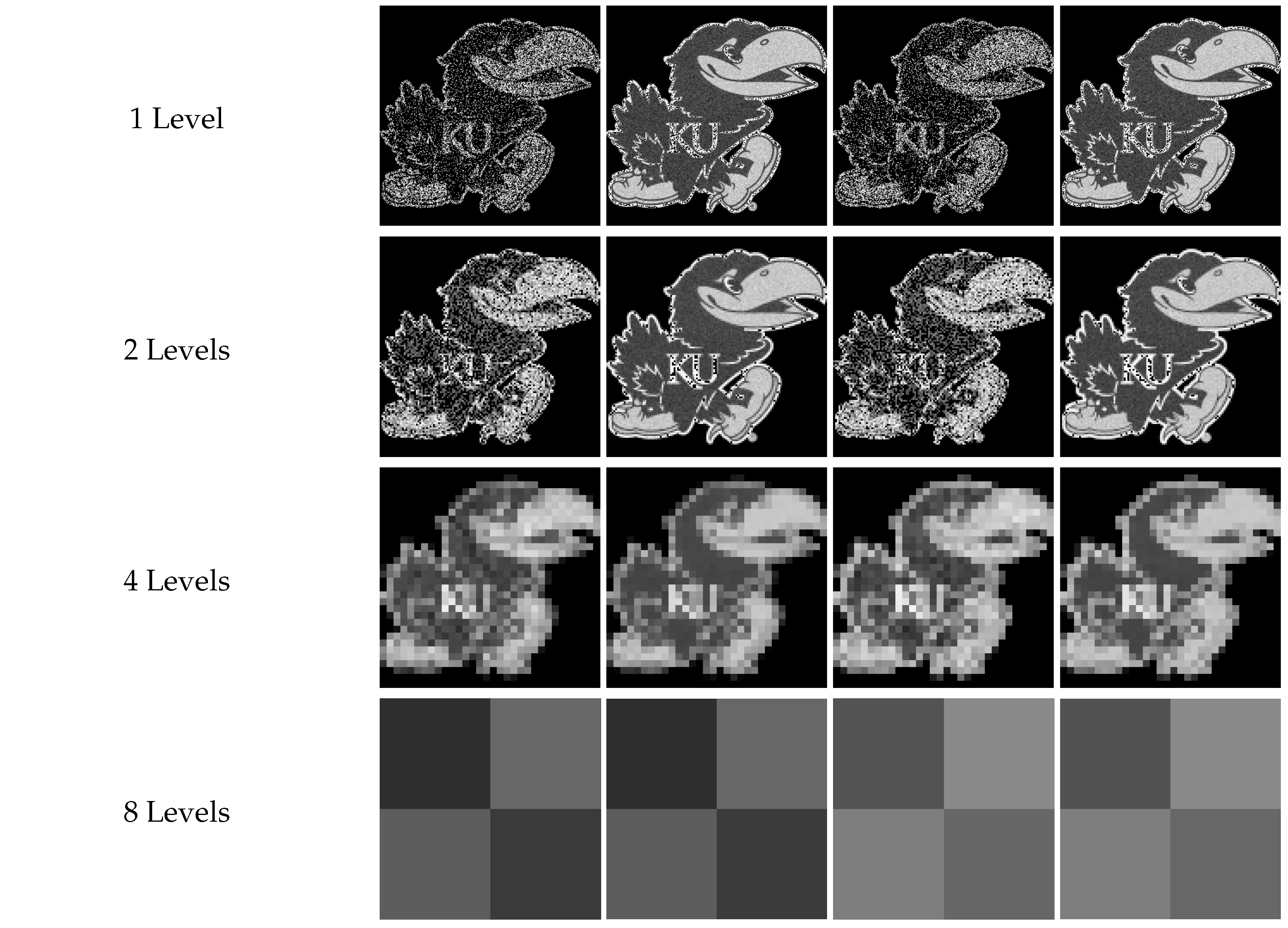 | ||||
Table 3.
Noisy outputs for 2-D Average and Euclidean Pooling on RGB (3-D) data of size () pixels.
| Levels of Decomposition | Average Pooling ( shots) |
Average Pooling ( shots) |
Euclidean Pooling ( shots) |
Euclidean Pooling ( shots) |
|---|---|---|---|---|
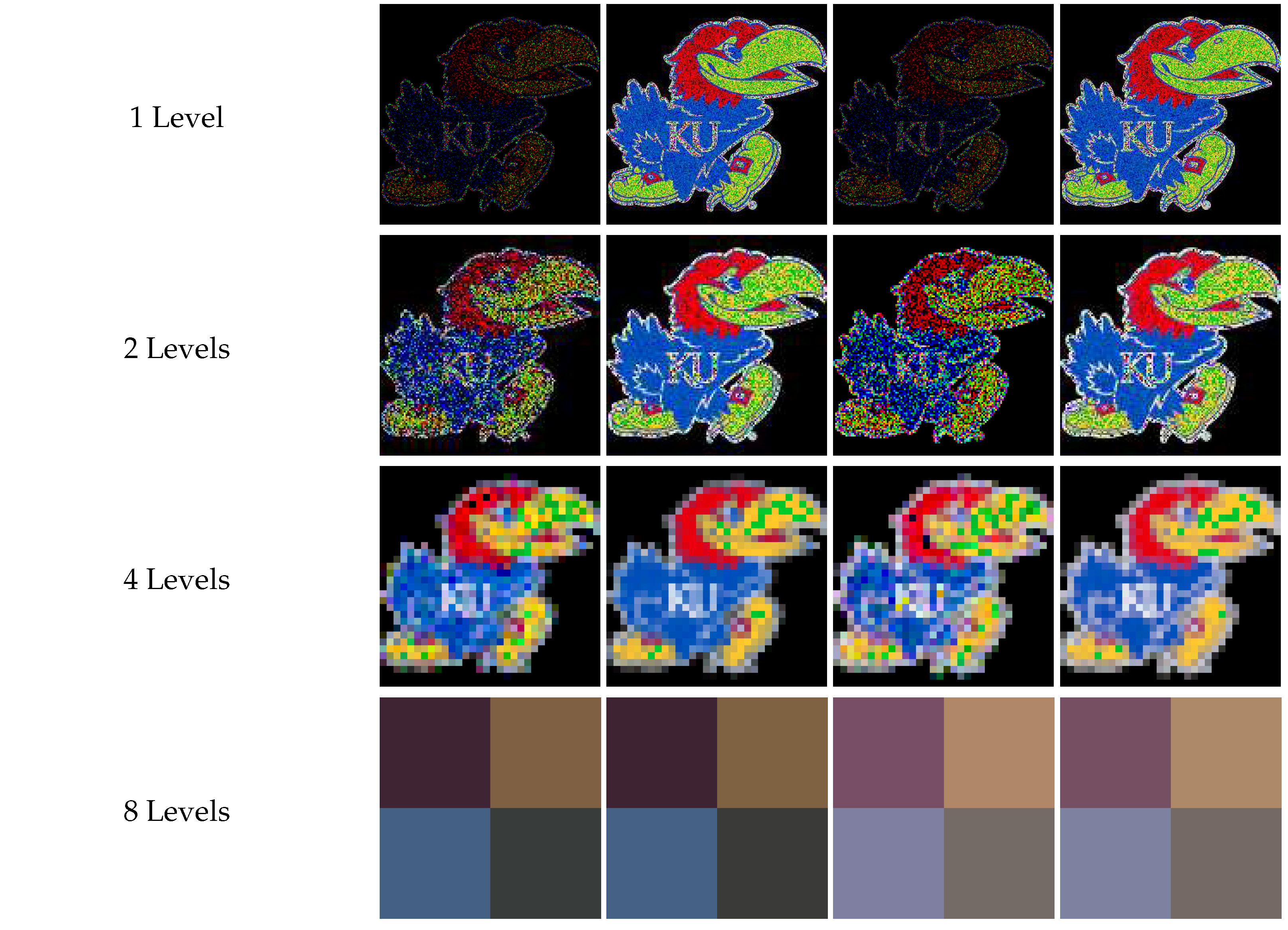 | ||||
Table 4.
Noisy outputs for 3-D Average and Euclidean Pooling on Hyperspectral (3-D) data of size () pixels.
Table 4.
Noisy outputs for 3-D Average and Euclidean Pooling on Hyperspectral (3-D) data of size () pixels.
| Levels of Decomposition | Average Pooling ( shots) |
Average Pooling ( shots) |
Euclidean Pooling ( shots) |
Euclidean Pooling ( shots) |
|---|---|---|---|---|
 | ||||
Disclaimer/Publisher’s Note: The statements, opinions and data contained in all publications are solely those of the individual author(s) and contributor(s) and not of MDPI and/or the editor(s). MDPI and/or the editor(s) disclaim responsibility for any injury to people or property resulting from any ideas, methods, instructions or products referred to in the content. |
© 2024 by the authors. Licensee MDPI, Basel, Switzerland. This article is an open access article distributed under the terms and conditions of the Creative Commons Attribution (CC BY) license (http://creativecommons.org/licenses/by/4.0/).
Copyright: This open access article is published under a Creative Commons CC BY 4.0 license, which permit the free download, distribution, and reuse, provided that the author and preprint are cited in any reuse.


