
Submitted:
06 January 2024
Posted:
08 January 2024
You are already at the latest version
Abstract
Tularemia is a zoonotic disease caused by {\it Francisella tularensis} bacteria, a gram-negative coccobacillus-shaped bacterium. There are multiple transmission routes of the infection to humans such as consumption of contaminated food or water, handling of infected animals or bites from {\it haematophagous} arthropods (such as ticks, deer flies, or mosquitoes). In this study we focus on transmission via the bites of ticks and developed a deterministic model of ordinary and impulsive differential equations to gain insight in the differential effect of prescribed fire on {\it Demacenta variablis} and {\it Amblyomma americanum} ticks and the prevalence of tularemina. We found that prescribed fire differentially reduce the number of the two ticks with {\it A. americanum} reduced the least compare to {\it D. variablis} subsequently leading to differential increase of tularemia new infected cases in humans and rodents. Our result further indicates that the spatial arrangement of burn against unburn areas may not matter as either arrangement led to fewer ticks and reduction in tularemia transmission when prescribed fire was implemented. The results of this study provide important new understandings of the intricate effect of prescribed fire on tick species, and the dynamics of the tick-borne disease, tularemia disease in this study.
Keywords:
prescribed fire
; amblyomma americanum
; demacenta variablis
; tularemia
; tick-borne disease
; sensitivity analysis
; multiple vectors
1. Introduction
Tick-borne diseases pose a growing public health concern, with their incidence on the rise in various regions around the world; generally tick-borne diseases, doubled from 2006 to 2018 [18,41]. For instance in the United States over 48,000 cases of tick-borne illnesses were reported in 2016 with close to 51,000 cases reported in 2019 [19]. These figures include reported cases from tick-borne diseases such as Lyme disease, anaplasmosis, Rocky Mountain spotted fever (RMSF), Babesiosis, ehrlichia chaffeensis ehrlichiosis, and Tularemia among others. The number of human Tularemia reported cases has been increasing in recent times in several countries from countries in North America (Canada, Mexico, United States), to several Nordic countries (Denmark, Norway, Sweden, Finland, and Iceland), and some Asian countries [14,87]. For instance, in Europe close to 1,500 cases of Tularemia disease were reported in 2019 with over 1,000 cases reported in 2016 [1]. Francisella tularensis is mostly distributed in the Northern hemisphere and is not normally found in the southern hemisphere or the tropics [1].
Tularemia has recently become a significant re-emerging disease in the world. Its low infectious dose, easy, high dissemination with aerosols, and the ability to induce fatal disease make Francisella tularensis a potential agent of biological warfare. This is why the Centers for Disease Control and Prevention (CDC) classified it as a category A biological weapon (Dennis et al. 2001; Maurin 2015) [87].
Tularemia is a zoonotic disease caused by Francisella tularensis bacteria [1,44,50,87], a gram-negative coccobacillus-shaped bacterium; it is also known as deer fly fever, Ohara’s fever, rabbit fever and Pahvant Valley plague [42,87]. There are four subspecies of Francisella tularensis namely tularensis (type A), holarctica (type B), novicida and mediasiatica [50,87]. The most virulent subspecies are tularensis and holarctica [1,32,50,53,62]. The subspecies tularensis, the most virulent of the two virulent subspecies, only occur in North America, while the subspecies holarctica is the most widespread of the subspecies, mediasiatica is present in central Asia, and novicida is the least virulent [1]. The subspecies tularensis and holarctica are the major etiological agents of tularemia in humans [87]. While the subspecies novicida is rarely associated with human infections [74,87], the subspecies mediasiatica have never been documented in published literature to cause infection in humans [87].
Transmission of francisella tularensis to humans occur via multiple routes, such as consumption of contaminated food or water, handling of infected animals or bites from haematophagous arthropod vectors (such as ticks, deer flies, or mosquitoes) [1,24,45]; other routes include contact with aquatic environment, and inhalation of aerosols [8,48,68,87]. Once an individual is infected with francisella tularensis, the incubation period ranges between 1–21 days [17,22,26,75,76,87]. The symptoms of tularemia include fever, fatigue, chills, and headache. The clinical manifestation of tularemia in humans depends on the site and route of acquisition of the infection[27,87]. There are six clinical forms of infection in humans, these include ulcero-glandular, glandular, oculo-glandular, oro-pharyngeal, pneumonic, and typhoidal forms [23,27,87].
Ulcero-glandular tularemia develops as a result of direct contact with an infected animal or a vector bite such as tick or deer fly; it leads to having skin lesions and lymphadenopathy. Although glandular and ulceroglandular tularemia are similar; however, glandular differs from ulceroglandular with the presence of regional lymphadenopathy with no detectable skin lesion. The oculo-glandular tularemia often develops via direct contact with contaminated water or splash of infected animal’s body fluids into the conjunctiva. Oro-pharyngeal result from ingestion of the bacterium and lead to symptoms such as pharyngitis, fever, and cervical lymphadenitis appear [70]. Pneumonic tularemia develops from the inhalation of infectious aerosols, while typhoidal tularemia develops from ingesting contaminated food and water. Moreover, pneumonic and typhoidal tularemia are considered systemic forms as they develop by the spread of bacteria through blood circulation as a systemic disease [87]. All six clinical forms of tularemia can cause secondary pleuropneumonia, meningitis, and sepsis, shock and death in infected individuals [4]. Tularemia is often diagnosed through the use of culture, serology, or molecular methods. The disease is frequently treated using quinolones, tetracyclines, or aminoglycosides. There are no licensed vaccine available for the prevention of tularemia [79,87].
The bacterium has a wide host range including different vertebrate groups as well as invertebrates [50,71]. However, rodents, hares, and rabbits are the principal vertebrate hosts [1], while ticks are the principal enzootic vector and reservoir and major sources of infection in human [1,61,87]. According to the Centers for Disease Control and Prevention (CDC), in the United States, tularemia disease can be transmitted to humans by three tick species namely Amblyomma americanum (lone Star tick), Dermacentor variabilis (american Dog tick) and Dermacentor andersoni (wood tick) [24]. In Europe, tularemia is transmitted by Dermacentor reticulatus [1]. Ticks goes through four developmental stages from eggs to larva to nymph, and then adult [6]. During each life stage, the ticks needs a blood meal to develop into the next stage of their life cycle [12].
Fire is considered a basic ecological process that keeps a variety of vegetative communities intact [47]. Prescribed fire or controlled burn is a common and essential land management technique in ecosystems that depend on fire, such as grasslands, open pine forests, and wetlands [31,83]. Prescribed fire are fire set by a group of professionals under specific weather conditions to restore health to ecosystems that depend on fire [13,81]. Prescribed fires are commonly used to control tick population in different environments by killing the ticks directly and destroying their leaf litter habitats [39]. Given the increase in recent decades of tick-borne diseases and the discovery of several new pathogens [59,73], it is necessity to identify cost-effective and practical methods for reducing the risk of tick-borne diseases. Gleim et al. [39], found that extended prescribed fires not only significantly decreased tick abundance but also altered the composition of tick species.
Our goal in this is to investigate the differential effect of fire on the tick -borne disease via a mathematical model. However, fewer modeling work have been done to consider the effect of prescribed fire on tick-borne diseases [35,41]. Guo and Agusto [41], investigated the effect of high and low intensity of prescribed fire on a single-vector tick-borne disease. The study presented a compartmental model for ticks carrying Lyme disease and incorporated the effects of prescribed fire using an impulsive system. They recommended that high-intensity prescribed burns done annually resulted in the most significant reduction in infectious nymphs, the primary carriers of Lyme disease [41]. Fulk et al. [35] also explored the effect of prescribed burns on the tick populations and the spread of Lyme disease by developing a spatial stage-structured tick-host model to simulate the impact of controlled burning on tick populations. The numerical simulations explained the effects of different numbers of burns and the time between burns on tick populations. However, it was again found that consistent prescribed burning at high intensity was the most effective control method for tick populations [35]. Furthermore, Fulk and Agusto [34] showed significant increase in the number of Ehrlichiosis infected Amblyomma americanum ticks at temperature increases in the absence of prescribed burning. However with prescribed burning, they observed a reduction in the prevalence of infectious ticks even as temperature increases to level such as C and C.
In this research work, we develop a compartmental model for a two-ticks two-hosts system with both tick species carrying Francisella tularensis and we investigate the differential effect of fire on the ticks and the prevalence of tularemia disease on the hosts. We are not aware of any studies considering the transmission of a single pathogen by multiple vectors. Although several studies have been done on a single-vector single-pathogen system [2,36,37,56,64,78,86] and co-infection of multiple pathogens in a single tick vector [54,77,80]. Also, some studies have considered single vector-multiple host system. For instance, Occhibove et al. [66] considered a single-vector, multi-host model for two tick species (Ixodes ricinus and Ixodes trianguliceps) individually infected with Borrelia burgdorferi and Babesia microti; the model further incorporated the ecological relationships with non-host species. The study aimed to understand the dynamics of tick-borne pathogens in pathosystems that differ in vector generalism. The study found that the degree of vector generalism affected pathogen transmission with different dilution outcomes. Norman et al. [65] also considered a two-hosts one-tick system with one host viraemic and the other not. They found that the non-viraemic hosts could either amplify the tick population leading to the persistence of the virus, or they may dilute the infection and cause it to die out.
The remainder of the work in this paper is organized as follows. In Section 2, we formulate our baseline tick/tularemia disease model, compute the model basic reproduction number, and carry out a global stability analysis including sensitivity analysis to determine the parameter with the most impact on the response function (basic reproduction number). In Section 3, we describe the tick model with the effect of prescribed fire using an impulsive system of ordinary differential equations and discuss prescribed fire related parameters estimated from literature. In Section 4, we carry out a global sensitivity analysis of the developed models. In Section 5, we present some simulation results, and in Section 6 we discuss our findings and close with conclusions.
2. Model Formulation
According to the Centers for Disease Control and Prevention, tularemia disease humans become infected when they are bitten by vector bite such as ticks or deer flies or by handling infected or deceased animals, or by the consumption of contaminated food or water. In this section, we formulate a model using non-linear ordinary differential equation that accounts for the interplay between humans (a dead end host, there is no evidence of human-to-human transmission), the American dog tick (referred to as tick 1), the lone star tick (referred to as tick 2) and rodents (pathogen reservoir). This model incorporates various compartments that depict the epidemiological state of each species in the system.
In the model, the human population is divided into susceptible exposed asymptomatic infected and recovered The total human population is denoted by and is defined as
The total rodent population is denoted by and is defined as
The tick population is divided by life stages, which include eggs, larvae, nymphs, and adults. Additionally, it is separated into susceptible and infected groups for larvae ( and ) and ( and ), nymphs ( and ) and ( and ), and adults ( and ) and and for tick 1 and tick 2, respectively. Since ticks must feed on blood to get infected, and there is no vertical transmission of the disease from parent ticks to their offspring, all tick eggs remain infection free ( and ).
For simplicity, we assume that human, tick and rodent populations are mixing homogeneously. The susceptible human sub-population are recruited at a rate The rate at which a susceptible human progress to the exposed class is denoted by and is defined as
This quantity is the force of infection for the humans, where and are the probabilities of transmission from tick 1 to human and tick 2 to human, respectively.
The incubation period for tularemia in humans ranges 1–21 days [17,22,26,75,76,87]. Furthermore, 4–19% of the infected human cases are asymptomatic [9,42]. Thus, the exposed human subsequently becomes either asymptomatic at a rate or infected at a rate with . Tularemia in humans is usually treated with antibiotics such as streptomycin, gentamicin, doxycycline, and ciprofloxacin [21]. Depending on the stage of illness and the type of medication used, treatment can last as long as 10–21 days with many of the patients completely recovering from the illness [21,49]. Hence, we assume that individuals who are infected as well as those who are asymptomatic both recover at the rate according to the reciprocal of the length of the treatment days. The human population is decreased by natural death at the rate denoted by and by disease induced mortality denoted by . The disease induced mortality rate for F. tularensis tularensis infections is about 30–35% and about 5–15% for F. tularensis holarctica infections when left untreated [49,60,76]. When treated with the appropriate antibiotics, these figure reduces to 1–3% [49,60]. The mortality rate in patients with typhoidal tularemia is higher than those of other forms of tularemia [60]. The case fatality rate of typhoidal tularemia if untreated is approximately 35%; it is the most dangerous form of tularemia infections [60]. Untreated ulceroglandular tularemia infection has a case fatality rate of 5% [60]. Permanent immunity usually develops after a single episode of tularemia [60].
For the rodent population, the recruited at a rate into the susceptible sub-population is denoted by . The rodents become infected following a bite from infected ticks of type 1 and 2 at the rate
where and are the probabilities of transmission from tick 1 to rodents and tick 2 to rodents, respectively. Rabbits, hares, and rodents often die in large numbers during outbreaks due to their high susceptibility to the bacteria [20]. The rodent population therefore is decreased by disease induced mortality denoted by and by natural death at the rate by .
For ticks, we assume that every adult tick can reproduce, regardless of whether they are susceptible or already infected, and that there is no vertical transmission of the bacteria to the eggs from infected females. The eggs develop into the larvae at rates and , with a certain proportion dying naturally at rates and for tick 1 and tick 2, respectively. The susceptible larvae of both tick 1 and tick 2 become infected larvae at a rate of and respectively or remain in the susceptible larval compartment. Thus, the force of infection in tick 1 and tick 2 (or the rate at which the ticks become infected after feeding on infected rodents) is given as
where and represents the probabilities that infections will occur when tick 1 or tick 2 bites an infected rodents. The populations of both susceptible and infected larvae are influenced by the natural mortality rate of for tick 1 and for tick 2. Regardless of their infection status, both susceptible and infected larvae from both tick species mature into their respective nymph stages at the rates and Following a subsequent infectious blood meal, susceptible nymphs in tick 1 and tick 2 become infected nymph at a rate of and respectively. The populations of both susceptible and infected nymphs from both tick species are reduced due to natural death rate of and and they mature into adults at the rate and respectively.
Given the assumptions above, the following nonlinear equations are given for the transmission dynamics of tularemia in two tick species:
The flow diagram for tularemia transmission is shown in Figure 1. The corresponding parameters and variables are described in Table 1 and Table 2.
2.1. Analysis of the Model
2.1.1. Basic Qualitative Properties
Positivity and Boundedness of Solutions
For the tularemia model (1) to be epidemiologically meaningful, it is important to prove that all its state variables are non-negative for all time. In other words, solutions of the model system (1) with non-negative initial data will remain non-negative for all time .
Lemma 1.
Let the initial data , where , where . Then the solutions of the tularemia model (1) are non-negative for all . Furthermore
where
and
The proof of Lemma 1 is given in Appendix A.
Invariant Regions
The tularemia model (1) will be analyzed in a biologically-feasible region as follows. Consider the feasible region
with,
and
Lemma 2.
The region is positively-invariant for the model (1) with non-negative initial conditions in .
The prove of Lemma 2 is given in Appendix B. In the next section, the conditions for the existence and stability of the equilibria of the model are stated.
2.1.2. Stability of Disease-Free Equilibrium (DFE)
The tularemia model has a disease-free equilibrium (DFE). The DFE is obtained by setting the right-hand sides and infected variables of the equation (2) to zero. The system has four equilibria . The equilibrium , involves humans and rodents only; while involves, humans, rodents and Demacenta variablis only; the equilirium involves humans, rodents and Amblyomma americanum only. Lastly, the involves humans, rodents and the two tick species. The expression for these equiliria are given as
where We will focus on the the stability of , the stability of the other equiliria can be determined using the same approach. Thus, the stability of can be established using the next generation operator method on system (1). Taking , and as the infected compartments and then using the aforementioned notation, the Jacobian F and V matrices for new infectious terms and the remaining transfer terms, respectively, are defined as:
where, . Therefore, using the definition of the reproduction number from [82] we have
where is the spectral radius and
The expressions and are the average number of secondary infections in rodents due to infectious Demacenta variablis and Amblyomma americanum while and are the average number of infections in ticks 1 and 2 due to an infectious rodents. Furthermore, using Theorem 2 in [82], the following result is established.
Lemma 3.
The disease-free equilibrium (DFE) of the tularemia model (1) is locally asymptotically stable (LAS) if and unstable if .
The quantity is basic reproduction number and it is defined as the average number of new infections that result from one infectious individual in a population that is fully susceptible. [5,30,46,82]. The epidemiological significance of Lemma 3 is that tularemia model (1) will be eliminated from within a herd if the reproduction number () can be brought to (and maintained at) a value less than unity.
3. Tick Model with Prescribed Fire
In this section, we consider the effect of fire on ticks and the rodent population, and the subsequent effect on the incidence and prevalence of the disease on humans. Note that fire is not explicitly incorporated into the tularemia model (1); rather, we consider the effect of fire on population size after the burns. To introduce the effect of prescribed fire into the tularemia disease model we have the following system of non-autonomous impulsive differential equations.
subject to the prescribed fire impulsive condition
where is the times that prescribed fire is implemented, which may be fixed or non-fixed; in this study we will consider the case with fixed times. The parameters are the proportion of tick type and mice population that is reduced by the fire. In Section 3.1 below, we discuss how these parameters are estimated using data from literature.
3.1. Estimating the Reduction Proportion Due to Prescribed Fire
To estimate the proportion (, , , , and ) reduced in the ticks and rodent populations due to fire, we used data from [38,67]. The study sites in [38] were located in Western Illinois University’s Alice L. Kibbe Field Station located in Warsaw, Hancock County, Illinois, USA. These sites consisted of several woodlands (oak-hickory, oak barrens), floodplain forests, restored tallgrass prairies and hill prairies. Low intensity burns were carried out at these sites; for low intensity burns, the heights of most flame were less than 1 meter and plant burnt were limited to the understory vegetation [85]. The last time the entire study site was burnt was in 2004 (B04) and two additional burns were later carried out in spring of 2014 (B14) and 2015 (B15).
Following the burns, ticks were collected by sweeping through the vegetation with a flannel cloth attached to a bamboo stick; this is known as flagging method. This was repeated every two weeks when the vegetation was dry between 12:00 and 18:00 hours from 9 May 2015 to 30 October 2015 and 22 April 2016 to 4 November 2016. To ensure tick mortality, the flannel cloth was placed in a sealed bag and frozen for three days. The ticks were later removed and identified using taxonomic keys, and their DNA extracted for pathogen testing. A total of 23 Dermacentor variabilis, 54 Ixodes scapularis, and 2788 Amblyomma americanum ticks were collected during the two consecutive years 2015 and 2016. A total of 23 D. variabilis were collected, (74%) were adults, (9%) were nymphs, and (17%) were larvae. For I. scapularis, 4% () of the 54 collected, were adults, 22% () were nymphs, and 74% (n = 40) were larvae. In the case of Amblyoma americanum, the ticks collected in B04 made up 51% of the collection (), while those collected in B14 made up 37% () of the collections, and those collected in B15 constituted 11% ) of the collection. Of these ticks, 2% () were adults, 4% () were nymphs, and 93% () were larvae. Although Ixodes scapularis were collected, we only estimate the parameters quantifying the reduction in the tick population due to fire using the data for Amblyoma americanum and Dermacentor variabilis since they are competent vector for the tuleramia.
Note that the study did not indicate if these were data for the pre-burn or post burn number of I. scapularis collected, nor did it provide data for the number of mice that were caught. So, we use the data for the rodent population provided in [67]. This study have data for six different rodent populations namely California kangaroo rat (Dipodomys californicus californicus), brush mouse (Peromyscus boylii), pinn mouse (P. truei sequoiensis), deer mouse (P. maniculatus gambelii), dusky-footed woodrat (Neotoma fuscipes), and western harvest mouse (Reithrodontomys megalotis longicaudus). After the fire treatment, about half as many rodents were trapped at the treated sites compared with control sites. At the two study sites (MG and DBP) only six tick species were found namely, Ixodes pacificus, Ixodes jellisoni, Ixodes spinipalpis, Ixodes woodi, Dermacentor occidentalis and Dermacentor parumapertus. The data for the Dermacentor subspecies (occidentalis and parumapertus) were not use in estimating the proportions since we are not aware of the transmission efficiency of these vectors unlike Dermacentor andersoni [24] which we do not have data for.
Estimating parameters : To estimate these parameters, we divide the numbers collected in each age group by the total number collected and subtract the proportion obtained from 1 to obtain the proportion reduced by fire. For instance, for Dermacentor variabilis, we have for the adult population. For nymphs it is , and for larvae. The proportion for Amblyoma americanum are similarly estimated as , , and . Lastly, the proportion for the rodent population using the data in [67] is given as .
4. Global Sensitivity Analysis
Sensitivity analysis procedure is often used to determine the impact and contribution of the model parameters to model outputs (such as the infected population)[7,25,43]. Results of the sensitivity analysis help to identify the best parameters to target for intervention or for future surveillance data gathering. We implement a global sensitivity analysis using Latin Hypercube Sampling (LHS) and partial rank correlation coefficients (PRCC) to assess the impact of parameter uncertainty and the sensitivity of these key model outputs. The LHS method is a stratified sampling technique without replacement this allows for an efficient analysis of parameter variations across simultaneous uncertainty ranges in each parameter [11,57,58,72]. The PRCC on the other hand measures the strength of the relationship between the parameters and the model outcome, stating the degree of the impact each parameter has on the model outcome [11,57,58,72].
We start by generating the LHS matrices and assuming all the model parameters are uniformly distributed except for the parameters representing number of burns (pulses) and the time between burns (). With these parameters we sampled their values from two pseudo-Poisson distributions that exclude zero as in [34,35]. For instance, Fulk et al. [34,35], sampled the values for pulses from a Poisson distribution centered on 10 (since they ran a scenario for 10 years) while was sampled from a Poisson distribution centered on 10. Once the initial distributions are created, “any zeros in either sample were changed to ones to avoid issues with implementing the burns" [34,35]. We then carry out a total of 1,000 simulations (runs) of the model for the LHS matrix, using the parameter values given in Table 2; the minimums and maximums for each parameter is set to of the baseline values respectively and the reproduction number () as the response function for tularemia model (1). We also considered other response functions at the end of the simulation for the tularemia models (1) and (2); these are the infected humans (), the infected rodents (), the sum of infected Demacenta variablis ticks in all life stages (), and the sum of infected Amblyomma americanum ticks in all life stages ().
4.1. Global Sensitivity Analysis for Tularaemia Model (1)
The outcome of the global sensitivity analysis for tularaemia model (1) using the reproduction number () is shown in Figure 2. The parameters with significant effect on the reproduction number are those parameters whose sensitivity index have significant p-values less than or equal to . The parameters with the most impacts on (), are rodent birth rate (), rodent transmission probability () to tick 2 (Amblyomma americanum), rodent death () and disease induced mortality () rate, A. americanum carrying capacity (), transmission probability () of tularemia to rodents from A. americanum, and the maturation rate () of A. americanum larvae and its adult death rate (. Notice that the parameters with significant effects on are related to the rodents and A. americanum.
For the other response functions (see Figure 3), the most significant parameters related to the infected humans, for instance are humans birth and death rates (, disease progression rate (), and the recovery rate (). For the infected rodent response function, the significant parameters are rodent transmission probability () to A. americanum and human disease induced death rate (). For the response function related to the sum of infected Demacenta variablis ticks in all life stages (), the significant parameters are the mortality rate () of adult D. variablis ticks, the maturation rate () of D. variablis nymphs, the mortality () and maturation () rates of larvae, eggs in-viability () and maturation () rates for D. variablis, and transmission probability () of D. variablis to rodents infection; finally for this response function is the rodent disease-induced death rate (). Lastly, for the sum of infected A. americanum ticks () response function, the significant parameters are the carrying capacity () of A. americanum, the transmission probability ) of A. americanum to-rodent, the eggs maturation () rate, the larvae maturation rate (), and the nymphs maturation () rate.
The PRCC index values of some of these parameters have positive signs while others have negative signs. The positive signs means that any increase in these parameters will lead to an increase in all the response functions. While the negative signs means that an increase in the parameters will lead to a decrease in the response functions. Hence, these parameters would be useful targets during mitigation efforts. Therefore, control strategies which targets these parameters with significant PRCC values will give the greatest impact on the model response functions.
4.2. Global Sensitivity Analysis for Tularaemia Model (2)
For the sensitivity analysis for tularaemia model (2), we included the number of burns (pulses) and the time between the burns () and drew from Poisson distributions for these parameters. We then used as response functions the sum of infected Demacenta variablis ticks in all life stages () and, the sum of infected Amblyomma americanum ticks in all life stages ().
For the two response functions, the number of burns (pulses) and the time between the burns () were the most significant parameters with negative and positive PRCC values followed by and . The sign on the pulses (negative) implies a negative impact on two ticks species. The sign on on the other hand is positive pointing to a positive impact on the ticks. In the next section below we will explore the impact of these two parameters on our model.
Thus, as the frequency of the burn increases few ticks will remain. That is, as the time between the burn increases more ticks will be found.
5. Numerical Simulations: Effect of Fire
Our goal in this research work is to investigate the differential effect of fire on the two tick species and the prevalence of tularemia disease on the two host populations (humans and rodents). To address our research goal, we simulate the tularemia model (2) with prescribed and compare the outcome to the tularemia model (1) without prescribe fire. We focus on infected humans, rodents, and the nymph populations of the two tick species.
In Figure 5 we observed a substantial difference between the number of humans and rodents infected with tularemia when prescribed fire is implemented and when it is absent (see Figure 5a,b). Although we have the same number of infected humans and rodents in the first year before the application of fire but once prescribed fire in implemented we see a reduction in infected humans and rodent population. We observed similar dynamics in both infected Demacenta variablis and Amblyomma americanum ticks but the population of A. americanum rebound quicker than those of D. variablis. Thus showing the differential effect of prescribed fire on the two tick species.
5.1. Differential Effect of Fire on Infected New Cases
Next we consider the differential effect of prescribed fire on cumulative humans and rodents infected new cases. To account for the cumulative number of new cases, we consider for humans the transition to the exposed class () from the susceptible class () due to the individual tick species. Similarly for the rodents, we consider the transition into the infected class () due to the individual ticks (see the force of infection for humans in models (1) and (2)). We then assumed all the ticks parameter values are the same except for the proportion reduced by fire. Figure 6 reveals the outcome of the simulation clearly showing the differential effect of fire. Furthermore, we observed the difference in the cumulative number of new cases due to the individual ticks, with Amblyomma americanum producing more infections than D. variablis, since many of them are remaining after each burn. Observe that in the absence of fire, the number of new cases from the infectious ticks of the two species are the same.
Next we simulate the models to show the differential effect of prescribed fire on the incidence of the disease due to individual tick species. Here the parameter values in Table 2 are used for the simulations and we can further see the differential effect of prescribed fire on the incidence of the disease.
5.2. Frequency and Time between Burn
Next, we consider the time between each burn and explore the effect of the frequency of the burn over ten years. We consider different burning regimes, for instance, we burn annually for a period of ten years, once every other year, once every five years, and once every ten years. We found in Figure 8 more infected humans and rodents as duration between burns increases. Similar increase in the number of infectious nymph populations is observed as the duration between each burn increases. However, the frequently prescribed fire is implemented the fewer the infected populations (humans, rodents, and ticks).
5.3. Burn Environments
Next, we consider the effect of burning in different environments. Using burn data Gleim et al. [39], we consider two additional environments, namely unburned area surrounded with burned area (UBB) and burned area surrounded by unburned area (BUB). This study did not collect data for the rodent population, so we used our baseline data obtained from [41,67] for the rodent population. We then simulate the tularemia model (2) and compare the results with no burn, UBB, BUB, and our baseline burn using data from [41,67].
In Figure 9, we observed almost similar number of infected Demacenta variablis ticks in the UBB and BUB environments. The ticks obtained in these environment are fewer in number than the number obtained in the baseline and unburned environments. For Amblyomma americanum ticks on the other hand, slightly more ticks were present in the UBB environment compared to the BUB, the baseline, and the no burn environments. This dynamics was also observed with the infected humans unlike the rodents that remained the same except for the no burn environment.
6. Discussion and Conclusion
Discussion
In this paper we developed and analyzed a mathematical model for a tick-borne tularemia disease transmission dynamics in humans, rodents and two ticks species (Demacenta variablis and Amblyomma americanum) using the natural history of infection of the disease; the model incorporates prescribed fire. Tularemia is a zoonotic disease caused by Francisella tularensis bacteria [1,44,50,87], a gram-negative coccobacillus-shaped bacterium; There are four subspecies of Francisella tularensis namely tularensis (type A), holarctica (type B),novicida and mediasiatica [50,87]. The most virulent subspecies are tularensis and holarctica [1,32,50,53,62]. The subspecies tularensis and holarctica are the major etiological agents of tularemia in humans [87]. There are multiple transmission routes of the infection to humans such as consumption of contaminated food or water, handling of infected animals or bites from haematophagous arthropod vectors (such as ticks, deer flies, or mosquitoes) [1,24,45]; other routes include contact with aquatic environment, and inhalation of aerosols [8,48,68,87]. In this study we focus on transmission via the bites of ticks.
The goal of the study is to explore the differential effect of fire via prescribed burn on the two ticks species and how that affects the prevalence of the disease in humans and rodents. Prescribed fire or controlled burn is a common and essential land management technique used in ecosystems that depend on fire, such as grasslands, open pine forests, and wetlands [31,83]. Prescribed fire was used often used by the native Americans long before the era of fire suppression. These practises are been revived by several native tribes across the United States [3,29]. These cultural fires help to repair degraded soil and increase biodiversity while reducing the leave litters and overgrowth that contributes to wild fires [3,29,84]. The native plants, which are adapted to fire are not harm by these cultural burns, in fact many of these plants need fire for their seeds to germinate [3].
Quantitative analysis of the tularemia model (1) without fire indicate that the model has a disease-free equilibrium that is locally asymptotically stable when the reproduction number is less than one. The global sensitivity analysis of this model using LHS/PRCC method was carried out to determine the parameter with the most influence on several response functions like the reproduction number (), the infected humans (), the infected rodents (), the sum of infected Demacenta variablis ticks in all life stages (), and the sum of infected Amblyomma americanum ticks in all life stages (). To implement the analysis, we used parameter values obtained from literature in most cases as well as assumed some where we could not find their values. Identification of these parameters are valuable for targeting interventions and perhaps for gathering data for other analyzes.
The parameters with the most significant impacts on the response functions are rodent birth rate (), rodent transmission probability () to Amblyomma americanum, rodent death () and disease induced mortality () rates, A. americanum carrying capacity (), transmission probability () of tularemia to rodents from A. americanum, and the maturation rate () of A. americanum larvae and its adult death rate ( (see Figure 2 and Figure 3). Others include humans birth and death rates (, disease progression rate (), and the recovery rate (), human disease induced death rate (). The significant parameters also include the mortality rate () of adult D. variablis ticks, the maturation rate () of D. variablis nymphs, the mortality () and maturation () rates of larvae, eggs in-viability () and maturation () rates for D. variablis, and transmission probability ( ) of D. variablis to rodents infection, rodent disease-induced death rate (), the eggs maturation () rate, the larvae maturation rate (), and the nymphs maturation () rate.
The sensitivity analysis for tularemia model (2) with prescribed fire was also carried out using as response functions the sum of infected D. variablis ticks () and the sum of infected A. americanum () ticks at all life stages as the model without fire; the number of burns (pulses) and the time between the burns () were drawn from Poisson distributions. For the two response functions, the number of burns (pulses) and the time between the burns () were the most significant parameters with PRCC values having negative and positive signs meaning negative and positive impact on the two ticks species. Thus, as the frequency of prescribed fire increases fewer ticks will remain or will be found. Furthermore, as the time between the burn increases more ticks will be found since their population would have increased in the time before the implementation of the next burn which will lead to reduction of their population. This result aligns with the outcome obtained by Guo and Agusto [41], and Fulk et al. [34,35].
Arthropods have complex reactions to fire [10]; their responses to fire depend on the intensity and severity of the fire. Fire can lead to abundance or reduction in their population and composition, so much so that only certain arthropods will be able to live in habitats that experience frequent fires especially wildfires [10]. In Figure 6 and Figure 7 we examine the differential effect of fire on the incidence of tularemia due to the two species using data collected by Gleim et al. [39,40]. The data showed more A. americanum than D. variablis were collected after the different burn regimes. This abundance was evident in the cumulative number of new human and rodent infection due to the tick species. To clearly show the differential effect of fire, we assumed the same parameter values for the two species except for the proportion reduced due to fire. As expected A. americanum which was reduced the least produced more infection, see Figure 6. In Figure 7, we relaxed this assumption and simulated the model using the parameters in Table 2; this figure further emphasis the result observed in Figure 7 that A. americanum led to more infection than D. variablis due to its abundance after the burn.
The numerical simulations of the tularaemia model (2) depicted in Figure 5, offer valuable insights into the dynamic interplay between prescribed fire and the spread of tularemia. The observed decrease in the number of infected, particularly in tick species D. variablis and A. americanum, underscores the potential efficacy of prescribed fire in mitigating the prevalence of the disease. This result aligns with the results obtained by Guo and Agusto [41] which showed reduction in Lyme diseased with the use of prescribed fire. Guo and Agusto [41] further showed that high intensity burn reduces more ticks than low intensity burn. This current study further aligns with study by Fulk et al. [35] which showed reduction in the prevalence of Lyme disease in different spatial setting (grassland or wooded area) with the application of prescribed burn. Similar results was also obtained in the study by Fulk and Agusto [34] on the effects of rising temperature and prescribed fire on Amblyomma Americanum with ehrlichiosis. The study found that with significant increase in temperature as high a 20C or 40C, implementing prescribed burning can still lead to reduction in the prevalence of infectious questing nymphs and adults with Ehrlichiosis.
Using the results from the sensitivity analysis we explore in Figure 8 the frequency and time between burns. The parameters used for the proportion reduced as a result of fire was obtained from [41,67]. Considering the results from Figure 8, there is a considerable reduction in infected humans and rodents as well as the infectious nymphs generally as a result of the burn. However, the frequency of the burn plays a significant role in ensuring whether there is a significant reduction or not. As can be deduced from the figure, one burn every year ensures a significant reduction in the infected (humans, rodents, and ticks).The simulation results emphasize the importance of well-timed fire applications in controlling tularemia. This result confirms the results from Guo and Agusto [41] which explore the effect of fire frequency and the time between burns. As identified in the study, the duration between burns has a more significant effect on ticks with higher-intensity fires than with lower-intensity fires. However, fire intensity appears to have a larger influence on tick reduction than the duration of the burns, as burning fewer times at a higher intensity is more effective than burning more times at a lower intensity.
The investigation of the different burn environments in Figure 9 reveals intriguing infection patterns in different burn environments (UBB and BUB). The number of infected was almost similar especially for D. variabilis and A. Americanum. Gleim et al. [39,40] indicted that frequent and long-term prescribed fire significantly reduces tick abundance at sites with varying burn regimes such as UBB and BUB. The results of this study suggests that the spatial arrangement of burned and unburned areas does not matter on the overall impact of prescribed fire on ticks and tularemia dynamics. This result may be affected by the fact that the same proportion of rodent population was used in the simulation of both environments. Considering the study done by Gleim et al. [39], a slightly different number of nymphs and adults of both species were obtained in both environment. Gleim et al. [39] research showed the differential effect of fire on these tick species; A. americanum is more fire tolerant than D. variablis; more A. americanum larvae were found in the two environments over none found for D. variablis. Our simulation results also shows this differential effect of fire on the two tick species, fewer nymphs of D. variablis remained at the end of our simulation period compare to the A. americanum remained.
6.1. Conclusion
To conclude, in this study we developed a deterministic model of ordinary and impulsive differential equations to gain insight in the differential effect of prescribed fire on Demacenta variablis and Amblyomma americanum ticks and the prevalence of tularemina. We found that prescribed fire can differentially reduce the number of the two ticks with D. variablis been reduced the most compare to A. americanum. We summarize the other results as follows:
- (i)
- The results of the sensitivity analyzes using as response or output functions the reproduction number (), the infected humans (), the infected rodents (), the sum of infected D. variablis ticks at all life stages (), and the sum of infected A. americanum ticks at all life stages () to identify the parameters with the most impact on these functions in no particular order are: the most significant parameters related infected humans are the birth, death, and disease induced death rates (, ), human disease progression rate (), and the recovery rate (); the most significant parameters related to infected rodents are rodent birth, death, and disease induced death rates (, , ), rodent transmission probability () to A. americanum. The significant parameters related D. variablis are eggs maturation () and in-viability () rates, the larvae maturation () and mortality () rates, the nymphs maturation rate (), and the adult mortality rate (). The significant parameters related to A. americanum are its carrying capacity (), the eggs maturation () rate, the larvae maturation rate (), and the nymphs maturation () rate, its adult death rate (, and the transmission probability () to rodents.
- (ii)
- Prescribed fire can reduce the number of ticks leading to a reduction in the number of tularemia infected humans, rodents and ticks.
- (iii)
- A. americanum produced more tulareamia infection in humans and rodents than D. variablis due to the differential effect of prescribed fire which leaves more A. americanum than D. variablis after a burn.
- (iv)
- As time between burn increases, more infected humans, rodents, and ticks increases. Frequent burning reduces the number of ticks and therefore infections.
- (v)
- The spatial arrangement of UBB and BUB areas may not matter as either arrangement led to fewer ticks and reduction in tularemia transmission with the implementation of prescribed fire.
In this study, we have used mathematical models to investigate the differential effect of prescribed burn on two tick species namely D. variablis and A. americanum and explored the effectiveness of prescribed fire in managing tick populations and lowering the prevalence of tularemia disease in the population (humans, rodents, and ticks). Our study is not without some limitations; the biggest drawbacks was the availability of data. For instance, there are no rodent data for the UBB and BUB environment. Despite this drawback, we have used the limited available data and we understand it might affect our results but we have confidence in our conclusions given the results from the sensitivity analysis we carried out.
Occhibove et al. [66] found that the degree of vector generalism affected pathogen transmission with different dilution outcomes. A. americanum is known as an aggressive and generalist hematophagous tick species [33,52,69]. In future studies, we will explore the differential effect of prescribed burn on the dilution or amplification tendencies of this tick species on the transmission dynamics of tick-borne diseases. Furthermore, we would also explore other ecological implications of our findings, by considering factors such as habitat fragmentation and species interactions in the presence of prescribed fire.
Acknowledgments
FBA is supported by the National Science Foundation under the EPSCOR Track 2 grant number 1920946.
Appendix A. Proof of Lemma 1
Lemma 1: Let the initial data , where , where ticks. Then the solutions of the tularemia model (1) are non-negative for all . Furthermore
where
and
Proof.
Let . Thus, . It follows from the first equation of the system (1), that
which can be re-written as
Hence,
so that,
Similarly, it can be shown that for all .
For the second part of the proof, note that , where ticks.
Hence,
as required. □
Appendix B. Proof of Lemma 2
Lemma 2: The region is positively-invariant for the tularemia model (1)-(2) with non-negative initial conditions in .
Proof.
Hence, , if . Thus,
In particular, if , then .
Hence, , if . Thus,
In particular, if , then .
Lastly, the ticks equations of the tularemia model (1) gives the following after summing the equations representing the eggs, larvae, nymphs, and adult stages for each of the ticks population
where and ticks. Thus,
Equations (B2), (B4), and (B6) implies that , and are bounded and all solutions starting in the region remain in . Thus, the region is positively-invariant and hence, the region attracts all solutions in .
□
References
- European Centre for Disease Prevention and Control (ECDC). Tularaemia: Annual epidemiological report for 2019. https://www.ecdc.europa.eu/en/publications-data/tularaemia-annual-epidemiological-report-2019, 2021. Accessed: 2023-12-14.
- Azmy, S. Ackleh and Amy Veprauskas. Modeling the invasion and establishment of a tick-borne pathogen. Ecological modelling, 467:109915, 2022.
- Molly Adams. KU professor leads students in prescribed burn at Lecompton prairie. https://lawrencekstimes.com/2023/11/29/cultural-burn-winter-school/, 2023. Accessed: 2023-12-28.
- American Veterinary Medical Association (AVMA). Tularemia facts. https://www.avma.org/tularemia-facts, 2003. Accessed: 2023-12-15.
- R.M. Anderson and R. May. Infectious Diseases of Humans. Oxford University Press, New York., 1991.
- Dmitry, A. Apanaskevich, J. H. Oliver, D. E. Sonenshine, and R. M. Roe. Life cycles and natural history of ticks. Biology of ticks, 1:59–73, 2014.
- R. B. Atherton, R. W. Schainker and E. R. Ducot. On the statistical sensitivity analysis of models for chemical kinetic. AIChE Journal, 21(3):441–448, 1975.
- Stina Bäckman, Jonas Näslund, Mats Forsman, and Johanna Thelaus. Transmission of tularemia from a water source by transstadial maintenance in a mosquito vector. Scientific reports, 5(1):7793, 2015.
- Genel Bir Bakış. A general overview of francisella tularensis and the epidemiology of tularemia in turkey. Flora, 15(2):37–58, 2010.
- Blyssalyn V Bieber, Dhaval K Vyas, Amanda M Koltz, Laura A Burkle, Kiaryce S Bey, Claire Guzinski, Shannon M Murphy, and Mayra C Vidal. Increasing prevalence of severe fires change the structure of arthropod communities: Evidence from a meta-analysis. Functional Ecology, 37(8):2096–2109, 2023.
- S. M. Blower and H. I. Dowlatabadi. Sensitivity and uncertainty analysis of complex models of disease transmission: an hiv model, as an example. International Statistical Review/Revue Internationale de Statistique, pages 229–243, 1994.
- N. Boulanger, P. Boyer, E. Talagrand-Reboul, and Y. Hansmann. Ticks and tick-borne diseases. Medecine et maladies infectieuses, 49(2):87–97, 2019.
- David M. J. S. Bowman, Jennifer K. Balch, Paulo Artaxo, William J. Bond, Jean M. Carlson, Mark A. Cochrane, Carla M. D’Antonio, Ruth S. DeFries, John C Doyle, and Sandy P Harrison. Fire in the earth system. science, 324(5926):481–484, 2009.
- Centers for Disease Control and Prevention (CDC). Tularemia: United states, 1990-2000. MMWR. Morbidity and mortality weekly report, 51(9):181–184, 2002.
- Centers for Disease Prevention and Control (CDC). Births and natality. https://www.cdc.gov/nchs/fastats/births.htm, 2023. Accessed: 2023-12-06.
- Centers for Disease Prevention and Control (CDC). Deaths and mortality. https://www.cdc.gov/nchs/fastats/deaths.htm, 2023. Accessed: 2023-12-06.
- Centers for Disease Prevention and Control (CDC). Frequently Asked Questions (FAQ) About Tularemia. https://emergency.cdc.gov/agent/tularemia/faq.asp#:~:text=Tularemia%2C%20also%20known%20as%20%E2%80%9Crabbit,all%20U.S.%20states%20except%20Hawaii., 2023. Accessed: 2023-11-30.
- Centers for Disease Prevention and Control (CDC). Tickborne disease surveillance data summary. https://www.cdc.gov/ticks/data-summary/index.html, 2023. Accessed: 2023-09-17.
- Centers for Disease Prevention and Control (CDC). Ticks: Tickborne disease surveillance data summary. https://www.cdc.gov/ticks/data-summary/index.html#print, 2023. Accessed: 2023-12-14.
- Centers for Disease Prevention and Control (CDC). Tularemia. https://www.cdc.gov/tularemia/index.html, 2023. Accessed: 2023-12-17.
- Centers for Disease Prevention and Control (CDC). Tularemia: Diagnosis & treatment. https://www.cdc.gov/tularemia/diagnosistreatment/index.html, 2023. Accessed: 2023-11-30.
- Centers for Disease Prevention and Control (CDC). Tularemia: For Clinicians. https://www.cdc.gov/tularemia/clinicians/index.html, 2023. Accessed: 2023-11-30.
- Centers for Disease Prevention and Control (CDC). Tularemia: Signs & symptoms. https://www.cdc.gov/tularemia/signssymptoms/index.html, 2023. Accessed: 2023-09-17.
- Centers for Disease Prevention and Control (CDC). Tularemia: Transmission. https://www.cdc.gov/tularemia/transmission/index.html, 2023. Accessed: 2023-12-15.
- Nakul Chitnis, James M. Hyman, and Jim M. Cushing. Determining important parameters in the spread of malaria through the sensitivity analysis of a mathematical model. Bulletin of mathematical biology, 70(5):1272–1296, 2008.
- Cleveland Clinic. Tularemia. https://my.clevelandclinic.org/health/diseases/17775-tularemia, 2023. Accessed: 2023-11-30.
- Columbia University, Lyme and Tick-Borne Diseases Research Center. Tularemia. https://www.columbia-lyme.org/tularemia, 2023. Accessed: 2023-11-30.
- L. M. Cooksey, D. G. Haile, and G. A. Mount. Computer simulation of rocky mountain spotted fever transmission by the american dog tick (acari: Ixodidae). Journal of medical entomology, 27(4):671–680, 1990.
- Max Diaz. Exploring the Benefits of Prescribed Fire. https://www.columbialandtrust.org/exploring-the-benefits-of-prescribed-fire/, 2023. Accessed: 2023-12-28.
- O. Diekmann, J. A. P. Heesterbeek, and J. A. P. Metz. On the definition and computation of the basic reproduction ratio r0 in models for infectious diseases in heterogeneous populations. Journal of Mathematical Biology, 28:503–522, 1990.
- Katherine J. Elliott, Ronald L. Hendrick, Amy E. Major, James M. Vose, and Wayne T. Swank. Vegetation dynamics after a prescribed fire in the southern appalachians. Forest Ecology and Management, 114(2-3):199–213, 1999.
- J. Ellis, P. C. Oyston, M. Green, and R. W. Titball. Tularemia. Clin Microbiol Rev, 15:631–646, 2002.
- Peter D. Fowler, S. Nguyentran, L. Quatroche, M. L. Porter, V. Kobbekaduwa, S. Tippin, Guy Miller, E. Dinh, E. Foster, and J. I. Tsao. Northward expansion of amblyomma americanum (acari: Ixodidae) into southwestern michigan. Journal of Medical Entomology, 59(5):1646–1659, 2022.
- A. Fulk and F. B. Agusto. Effects of rising temperature and prescribed fire on amblyomma americanum with ehrlichiosis. medRxiv, pages 2022–11, 2022.
- A. Fulk, W. Huang, and F. B. Agusto. Exploring the effects of prescribed fire on tick spread and propagation in a spatial setting. Computational and Mathematical Methods in Medicine, 2022, 2022.
- Holly Gaff and Elsa Schaefer. Metapopulation models in tick-borne disease transmission modelling. Modelling parasite transmission and control, pages 51–65, 2010.
- Holly D. Gaff and Louis J. Gross. Modeling tick-borne disease: a metapopulation model. Bulletin of Mathematical Biology, 69:265–288, 2007.
- M. E. Gilliam, Will T. Rechkemmer, K. W. McCravy, and S. E. Jenkins. The influence of prescribed fire, habitat, and weather on Amblyomma americanum (Ixodida: Ixodidae) in West-Central Illinois, USA. Insects, 9(2):36, 2018.
- E. R. Gleim, L. M. Conner, R. D. Berghaus, M. L. Levin, G. E. Zemtsova, and M. J. Yabsley. The phenology of ticks and the effects of long-term prescribed burning on tick population dynamics in southwestern Georgia and northwestern Florida. PLoS One, 9(11):e112174, 2014.
- Elizabeth R. Gleim, Galina E. Zemtsova, Roy D. Berghaus, Michael L. Levin, Mike Conner, and Michael J. Yabsley. Frequent prescribed fires can reduce risk of tick-borne diseases. Scientific reports, 9(1):9974, 2019.
- E. Guo and F. B. Agusto. Baptism of fire: Modeling the effects of prescribed fire on lyme disease. Canadian Journal of Infectious Diseases and Medical Microbiology, 2022, 2022.
- Gürcan. Epidemiology of tularemia. Balkan medical journal, 2014(1):3–10, 2014.
- D.M. Hamby. A review of techniques for parameter sensitivity analysis of environmental models. Environmental monitoring and assessment, 32(2):135–154, 1994.
- M. J. Hepburn and A. J. H. Simpson. Tularemia: current diagnosis and treatment options. Expert review of anti-infective therapy, 6(2):231–240, 2008.
- G. Hestvik, E. Warns-Petit, L. A. Smith, N. J. Fox, H. Uhlhorn, M. Artois, D. Hannant, M. R. Hutchings, R. Mattsson, and L. Yon. The status of tularemia in europe in a one-health context: a review. Epidemiology & Infection, 143(10):2137–2160, 2015.
- H. W. Hethcote. The mathematics of infectious diseases. SIAM Review, 42(4):599–653, 2000.
- J. Kevin Hiers, Joseph J. O’Brien, J. Morgan Varner, Bret W. Butler, Matthew Dickinson, James Furman, Michael Gallagher, David Godwin, Scott L. Goodrick, and Sharon M. Hood. Prescribed fire science: The case for a refined research agenda. Fire Ecology, 16:1–15, 2020.
- C. E. Hopla. The ecology of tularemia. Advances in veterinary science and comparative medicine, 18:25–53, 1974.
- Illinois Department of Public Health. Tularemia. https://dph.illinois.gov/topics-services/emergency-preparedness-response/public-health-care-system-preparedness/tularemia, 2023. Accessed: 2023-11-30.
- Sonja Kittl, Thierry Francey, Isabelle Brodard, Francesco C. Origgi, Stéphanie Borel, Marie-Pierre Ryser-Degiorgis, Ariane Schweighauser, and Joerg Jores. First european report of francisella tularensis subsp. holarctica isolation from a domestic cat. Veterinary research, 51(1):1–5, 2020.
- C. J. Krebs. Ecological methodology. Addison-Wesley Educational Publishers, Inc., 1989.
- Deepak Kumar, Surendra Raj Sharma, Abdulsalam Adegoke, Ashley Kennedy, Holly C. Tuten, Andrew Y. Li, and Shahid Karim. Recently evolved francisella-like endosymbiont outcompetes an ancient and evolutionarily associated coxiella-like endosymbiont in the lone star tick (amblyomma americanum) linked to the alpha-gal syndrome. Frontiers in Cellular and Infection Microbiology, 12:425, 2022.
- Marilynn A. Larson, Khalid Sayood, Amanda M. Bartling, Jennifer R. Meyer, Clarise Starr, James Baldwin, and Michael P. Dempsey. Differentiation of francisella tularensis subspecies and subtypes. Journal of clinical microbiology, 58(4):10–1128, 2020.
- Y. Lou, L. Liu, and D. Gao. Modeling co-infection of ixodes tick-borne pathogens. Mathematical Biosciences & Engineering, 14(5&6):1301, 2017.
- A. Ludwig, H.S. Ginsberg, G.J. Hickling, and N.H. Ogden. A dynamic population model to investigate effects of climate and climate-independent factors on the lifecycle of amblyomma americanum (acari: Ixodidae). Journal of Medical Entomology, 53(1):99–115, 2016.
- Milliward Maliyoni, Faraimunashe Chirove, Holly D. Gaff, and Keshlan S. Govinder. A stochastic tick-borne disease model: Exploring the probability of pathogen persistence. Bulletin of mathematical biology, 79:1999–2021, 2017.
- Marino, I. B. Hogue, C. J. Ray, and D. E. Kirschner. A methodology for performing global uncertainty and sensitivity analysis in systems biology. Journal of theoretical biology, 254(1):178–196, 2008.
- M. D. McKay, R. J. Beckman, and W. J. Conover. A comparison of three methods for selecting values of input variables in the analysis of output from a computer code. Technometrics, 42(1):55–61, 2000.
- Laura K. McMullan, Scott M. Folk, Aubree J. Kelly, Adam MacNeil, Cynthia S. Goldsmith, Maureen G. Metcalfe, Brigid C. Batten, César G. Albariño, Sherif R. Zaki, and Pierre E. Rollin. A new phlebovirus associated with severe febrile illness in missouri. New England Journal of Medicine, 367(9):834–841, 2012.
- Medscape. Tularemia. https://emedicine.medscape.com/article/230923-overview?form=fpf, 2023. Accessed: 2023-11-30.
- T. Mörner. The ecology of tularaemia. Revue scientifique et technique (International Office of Epizootics), 11(4):1123–1130, 1992.
- Torsten Mörner and Edward Addison. Tularemia. Infectious diseases of wild mammals, pages 303–312, 2001.
- G. A. Mount and D. G. Haile. Computer simulation of population dynamics of the american dog tick (acari: Ixodidae). Journal of medical entomology, 26(1):60–76, 1989.
- H. G. Mwambi, J. Baumgärtner, and K. P. Hadeler. Ticks and tick-borne diseases: a vector-host interaction model for the brown ear tick (rhipicephalus appendiculatus). Statistical Methods in Medical Research, 9(3):279–301, 2000.
- R. Norman, R.G. Bowers, M. Begon, and .J. Hudson. Persistence of tick-borne virus in the presence of multiple host species: tick reservoirs and parasite mediated competition. Journal of theoretical biology, 200(1):111–118, 1999.
- F. Occhibove, K. Kenobi, M. Swain, and C. Risley. An eco-epidemiological modeling approach to investigate dilution effect in two different tick-borne pathosystems. Ecological Applications, 32(3):e2550, 2022.
- K. A. Padgett, L. E. Casher, S. L. Stephens, and R. S. Lane. Effect of prescribed fire for tick control in california chaparral. Journal of Medical Entomology, 46(5):1138–1145, 2009.
- Stephen R. Palmer, Lord Soulsby, and David Ian Hewitt Simpson. Zoonoses: biology, clinical practice, and public health control. Oxford university press, 1998.
- Emily L. Pascoe, Matteo Marcantonio, Cyril Caminade, and Janet E. Foley. Modeling potential habitat for amblyomma tick species in california. Insects, 10(7):201, 2019.
- Robert, L. Penn. Francisella tularensis (tularemia). In Mandell, Douglas, and Bennett’s principles and practice of infectious diseases, pages 2590–2602. Elsevier, 2015.
- Paola Pilo. Phylogenetic lineages of francisella tularensis in animals. Frontiers in cellular and infection microbiology, 8:258, 2018.
- M. A. Sanchez and S. M. Blower. Uncertainty and sensitivity analysis of the basic reproductive rate: tuberculosis as an example. American Journal of Epidemiology, 145(12):1127–1137, 1997.
- Harry M. Savage, Kristen L. Burkhalter, Marvin S. Godsey Jr, Nicholas A. Panella, David C. Ashley, William L. Nicholson, and Amy J. Lambert. Bourbon virus in field-collected ticks, missouri, usa. Emerging Infectious Diseases, 23(12), 2017.
- A Sjöstedt. Family xvii. francisellaceae, genus i., 2005.
- J. Snowden and K. A. Simonsen. Tularemia. https://europepmc.org/books/n/statpearls/article-30676/?extid=28613501&src=med, 2023. Accessed: 2023-11-30.
- State of New Jersey, Department of Agriculture. Tularemia. https://www.nj.gov/agriculture/divisions/ah/diseases/tularemia.html, 2023. Accessed: 2023-11-30.
- Bei Sun, Xue Zhang, and Marco Tosato. Effects of coinfection on the dynamics of two pathogens in a tick-host infection model. Complexity, 2020:1–14, 2020.
- Olivia Tardy, Catherine Bouchard, Eric Chamberland, André Fortin, Patricia Lamirande, Nicholas H. Ogden, and Patrick A. Leighton. Mechanistic movement models reveal ecological drivers of tick-borne pathogen spread. Journal of the Royal Society Interface, 18(181):20210134, 2021.
- A. Tärnvik and M. C. Chu. New approaches to diagnosis and therapy of tularemia. Annals of the New York Academy of Sciences, 1105(1):378–404, 2007.
- Danielle M. Tufts, Ben Adams, and Maria A. Diuk-Wasser. Ecological interactions driving population dynamics of two tick-borne pathogens, borrelia burgdorferi and babesia microti. Proceedings of the Royal Society B, 290(2001):20230642, 2023.
- US Forest Service, U.S. Department of Agriculture. Prescribed fire. https://www.fs.usda.gov/managing-land/prescribed-fire, 2023. Accessed: 2023-12-10.
- P. Van den Driessche and J. Watmough. Reproduction numbers and sub-threshold endemic equilibria for compartmental models of disease transmission. Mathematical biosciences, 180(1):29–48, 2002.
- J. Morgan Varner, Mary A. Arthur, Stacy L. Clark, Daniel C. Dey, Justin L. Hart, and Callie J. Schweitzer. Fire in eastern north american oak ecosystems: filling the gaps. Fire Ecology, 12:1–6, 2016.
- VOA News. 'Prescribed Burns' Could Aid Forests in US Southeast, Experts Say. https://www.voanews.com/a/prescribed-burns-could-aid-forests-in-us-southeast-experts-say-/7399183.html, 2023. Accessed: 2023-12-28.
- Robert J. Whelan. The ecology of fire. Cambridge university press, 1995.
- Michael C. Wimberly, Adam D. Baer, and Michael J. Yabsley. Enhanced spatial models for predicting the geographic distributions of tick-borne pathogens. International Journal of Health Geographics, 7(1):1–14, 2008.
- Derya Karataş Yeni, Fatih Büyük, Asma Ashraf, and M. Salah ud Din Shah. Tularemia: a re-emerging tick-borne infectious disease. Folia microbiologica, 66(1):1–14, 2021.
Figure 1.
Flow diagram of the Tularemia model (1).
Figure 1.
Flow diagram of the Tularemia model (1).
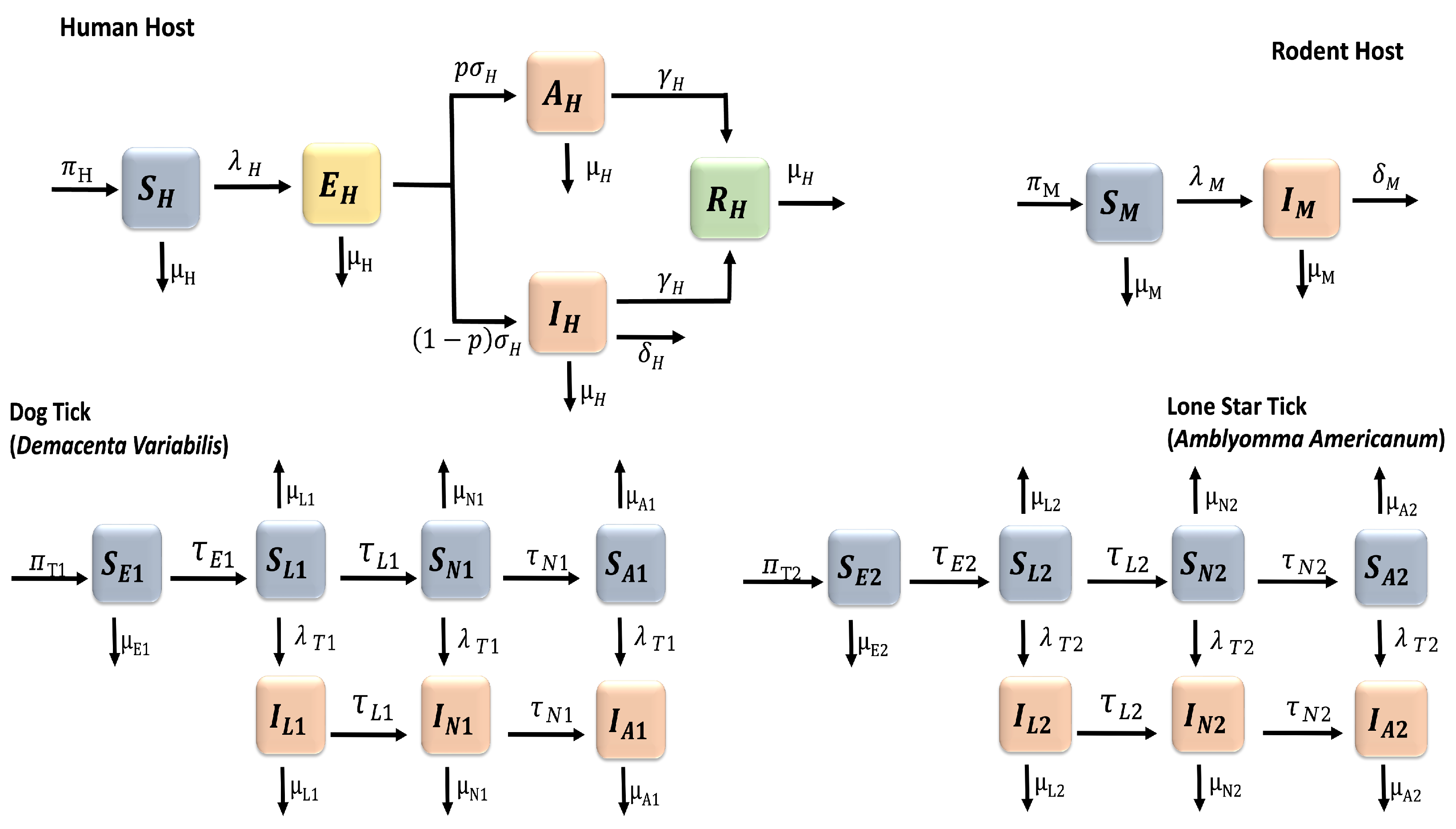
Figure 2.
PRCC values for the tularaemia model (1), using the reproduction number as response functions and parameter values in Table 2 with ranges that are from the baseline values.
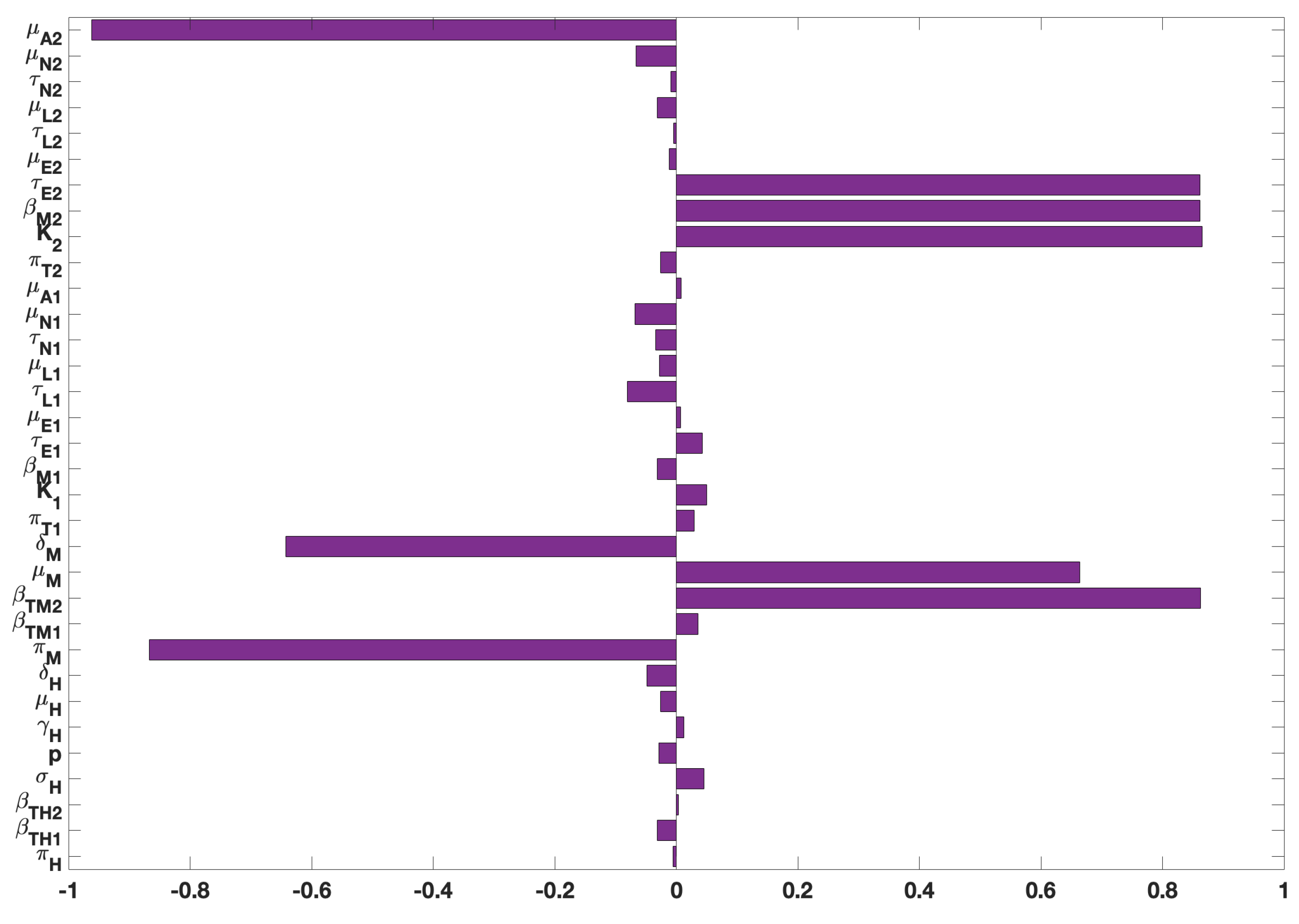
Figure 3.
PRCC values for the tularaemia model (1), using as response functions: (a) The infected humans (); (b) The infected rodents (); (c) The sum of infected Demacenta variablis ticks in all life stages (); and ; (d) The sum of infected Amblyomma americanum ticks in all life stages (). Using parameter values in Table 2 and ranges that are from the baseline values.
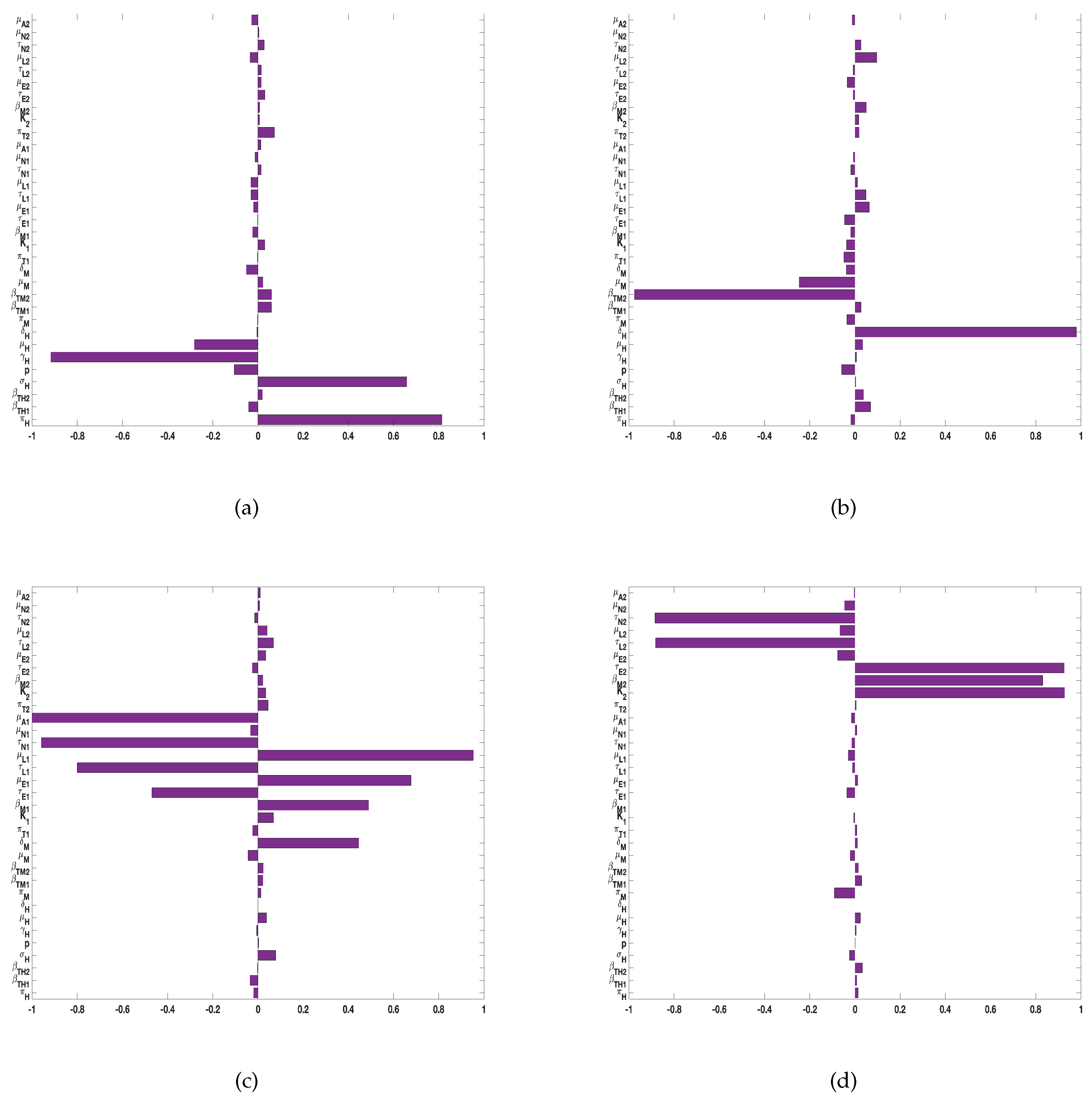
Figure 4.
PRCC values for the tularaemia model (1), using as response functions: (a) The sum of infected Demacenta variablis ticks at all life stages (); and (b) The sum of infected Amblyomma americanum ticks at all life stages (). Using parameter values in Table 2 and ranges that are from the baseline values.
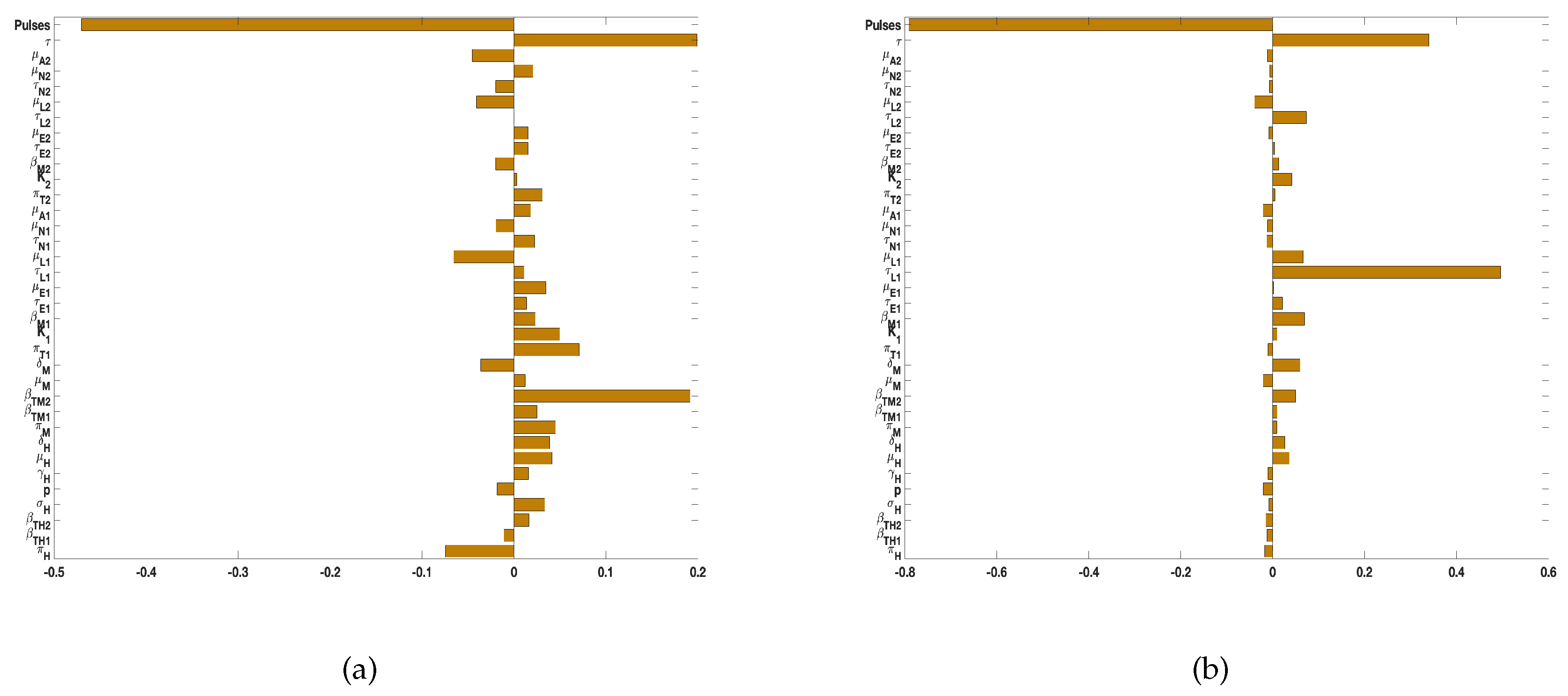
Figure 5.
Simulation of tularaemia model (1) showing the effect of prescribed fire on: (a) Infected humans (); (b) Infected rodents (); (c) Infected Demacenta variablis (); and (d) Infected Amblyomma americanum (). Using parameter values in Table 2.
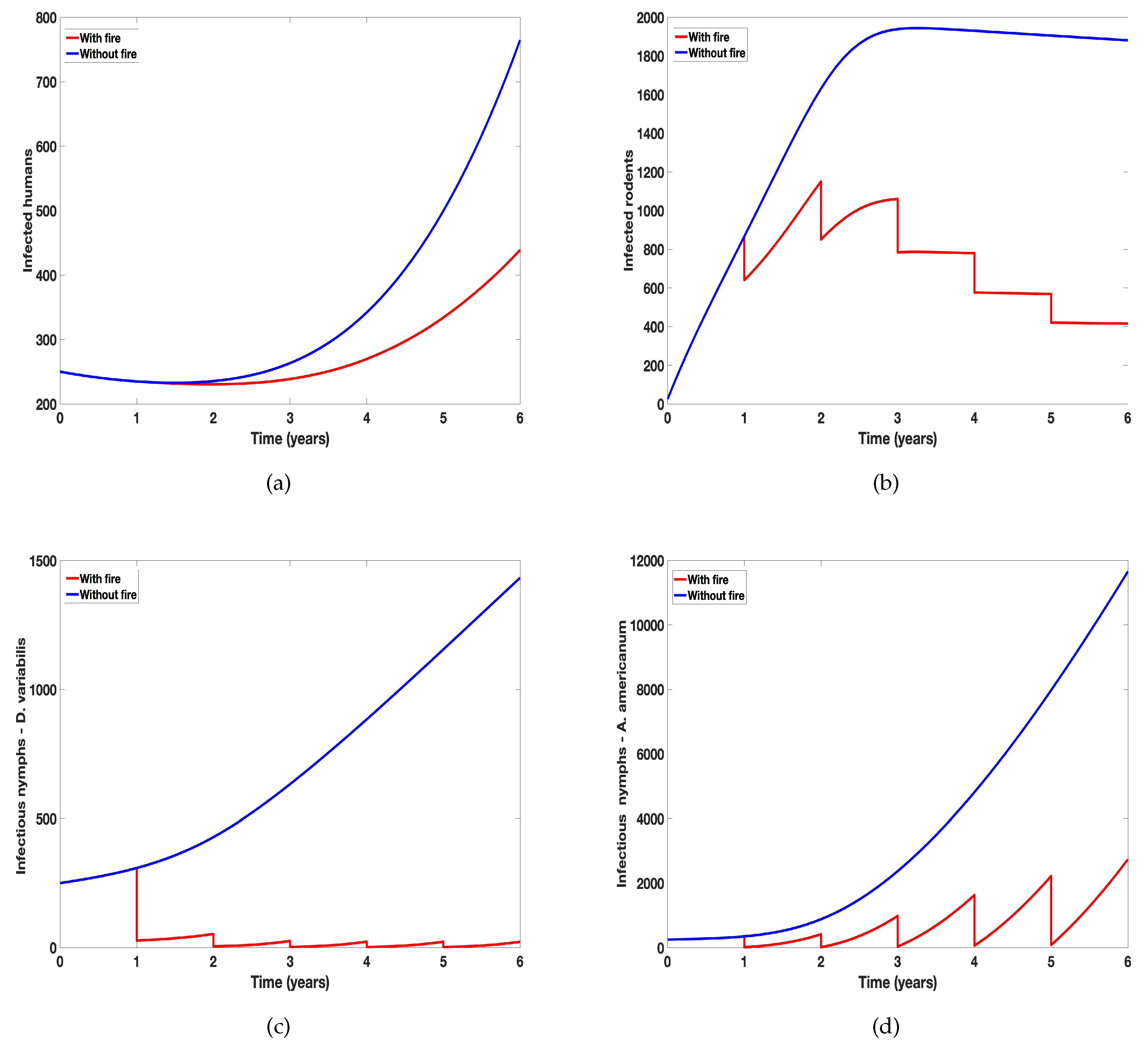
Figure 6.
Simulation of tularaemia models (1) and (2) showing differential effect of prescribed fire on: (a) Cumulative number of new infected humans cases; (b) Cumulative number of new infected rodents cases. Using parameter values in Table 2 and assuming the ticks related parameter values for the two tick species are the same.
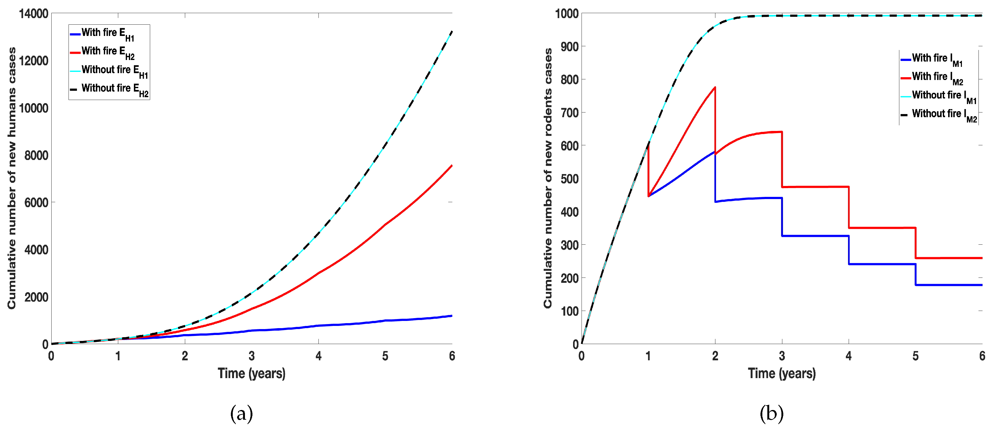
Figure 7.
Simulation of tularaemia models (1) and (2) showing differential effect of prescribed fire on: (a) Cumulative number new infected humans cases in the absence of fire; (b) Cumulative number of new infected humans cases in the presence of fire; ; (c) Cumulative number of new infected rodents cases in the absence of fire; and (d) Cumulative number of new infected rodents cases in the presence of fire. Using parameter values in Table 2.
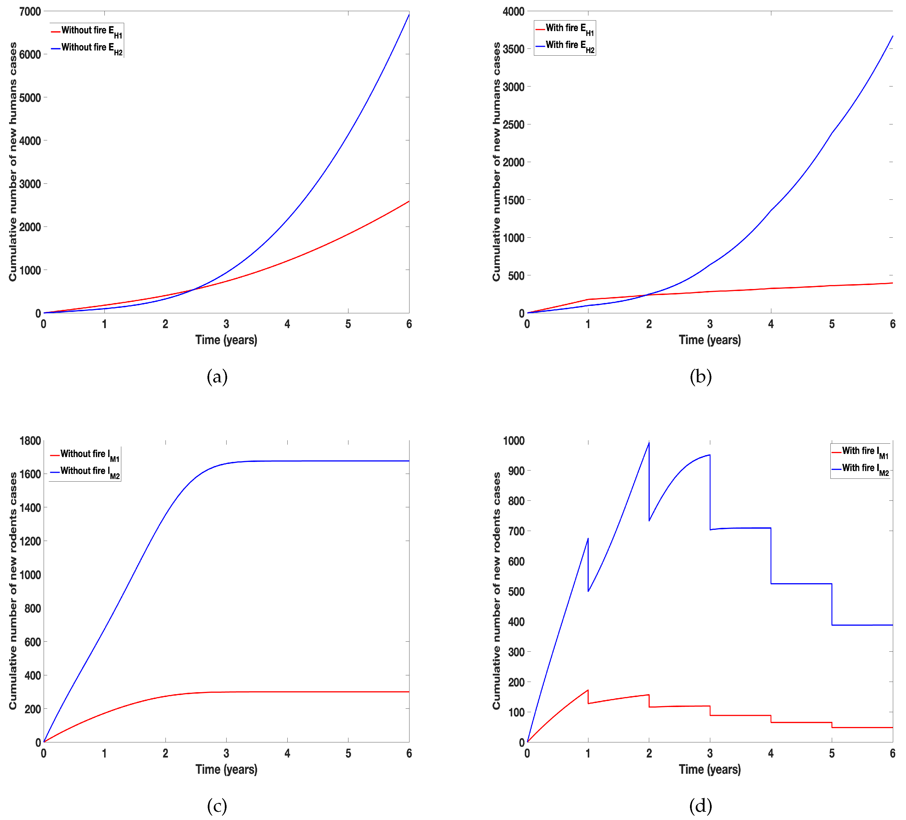
Figure 8.
Simulation of tularaemia model (2) with prescribed fire with different time between burn using the baseline prescribed fire reduction parameters obtained from [41,67] and the rest of the parameter values in Table 2.
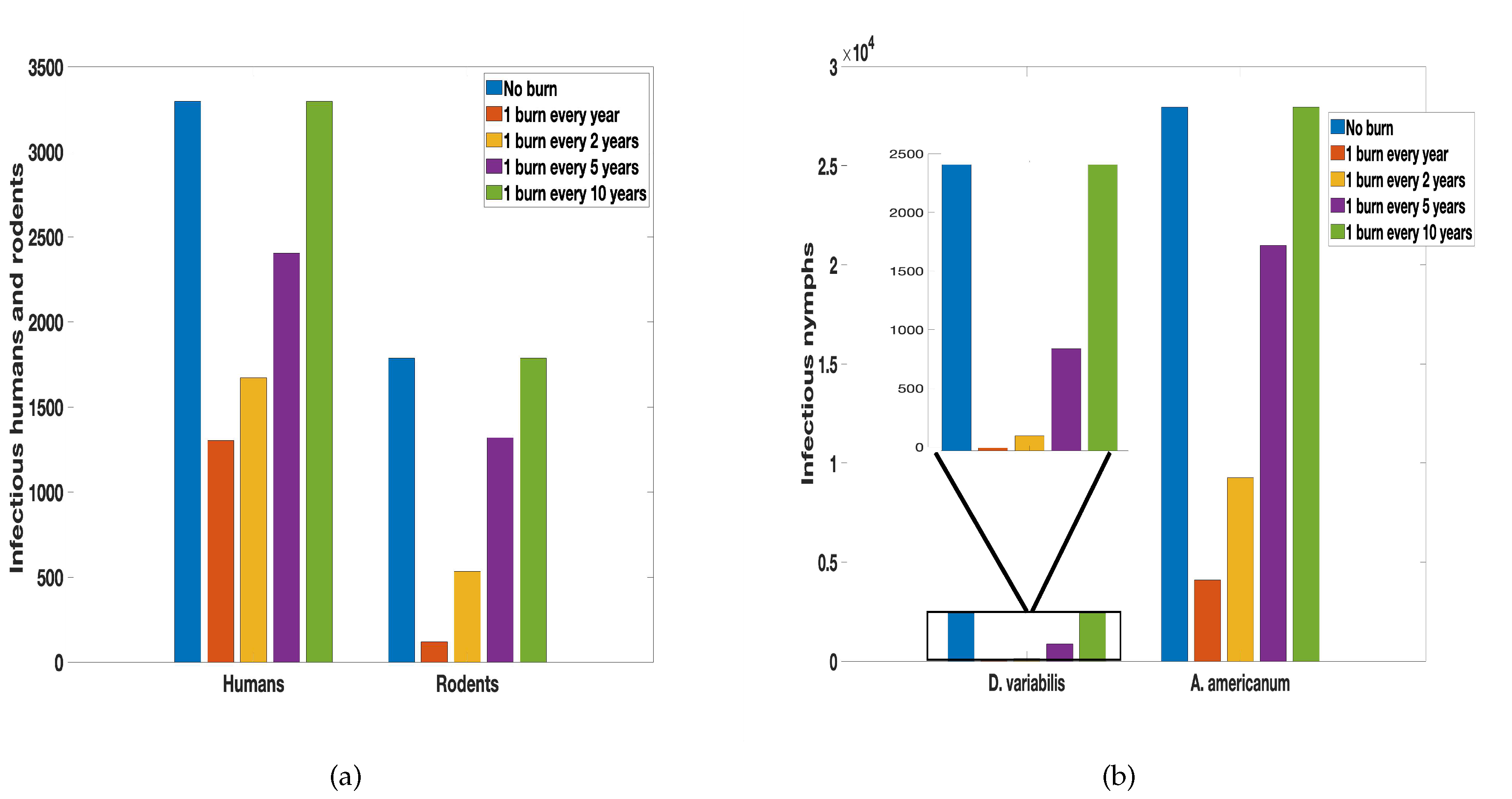
Figure 9.
Simulation of tularaemia model (2) with prescribed fire in different environments using the baseline prescribed fire reduction parameters obtained from [41,67] and parameters from Gleim et al. [39] where UBB stands for unburn area surrounded by burn area; BUB is burn area surround by unburn area. The reduction due to fires in UBB and BUB were estimated from [39], the rest of the parameter values in Table 2.
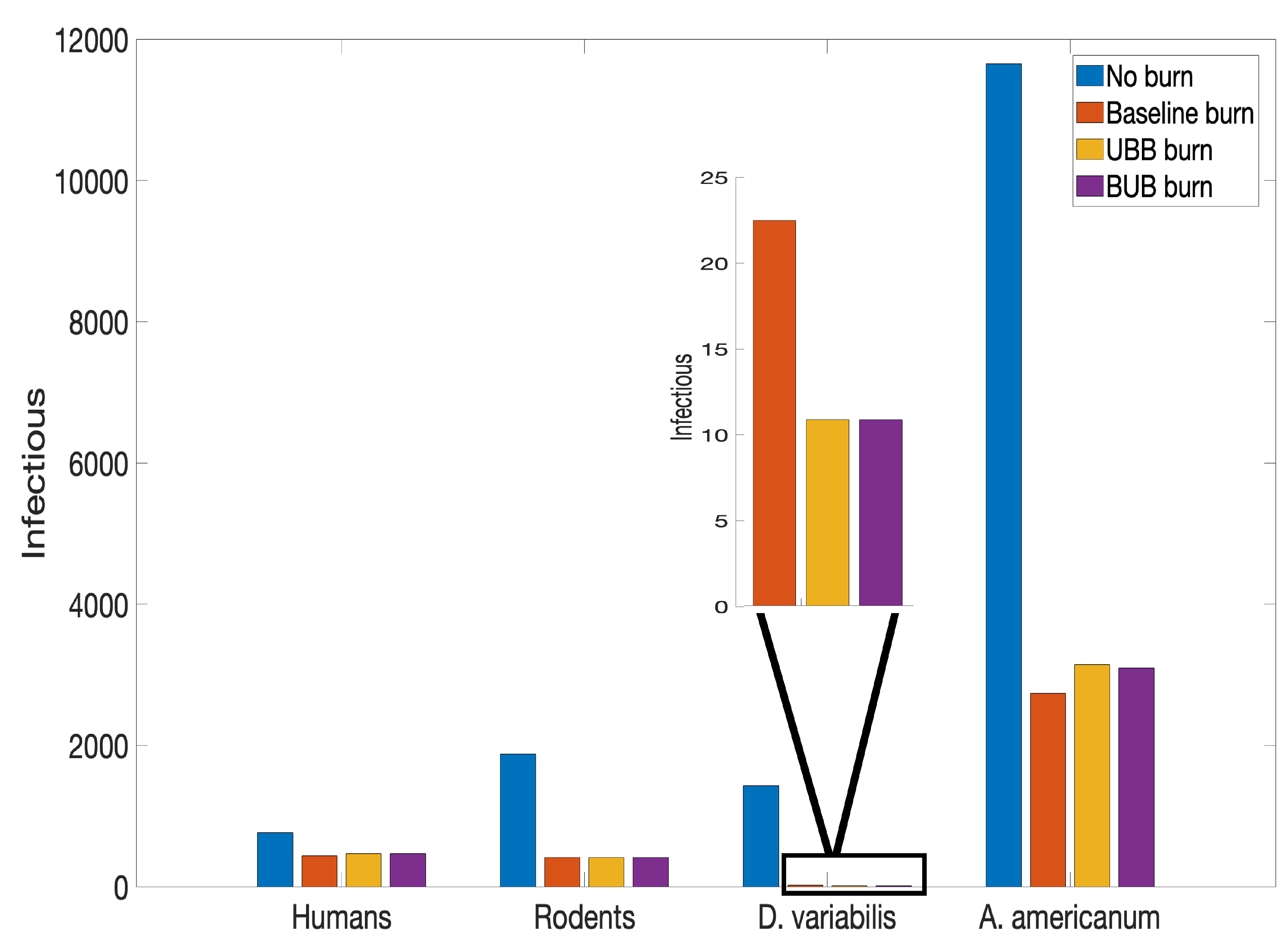

Table 1.
Description of the tularemia model (1) variables, where tick 1 represent Demacenta variablis and tick 2 represent Amblyomma americanum.
Table 1.
Description of the tularemia model (1) variables, where tick 1 represent Demacenta variablis and tick 2 represent Amblyomma americanum.
| Variable | Description |
|---|---|
| Number of susceptible humans | |
| Number of exposed humans | |
| Number of asymptomatic humans | |
| Number of infected humans | |
| Number of recovered humans | |
| Number of susceptible rodents | |
| Number of infected rodents | |
| Number of susceptible eggs of ticks type | |
| Number of susceptible larvae of ticks type i | |
| Number of infected larvae of ticks type i | |
| Number of susceptible nymphs of ticks type i | |
| Number of infected nymphs of ticks type i | |
| Number of susceptible adults of ticks type i | |
| Number of infected adults of ticks type i |
Table 2.
Description and values of the tularemia model (1) parameters, where tick 1 represent Demacenta variablis and tick 2 represent Amblyomma americanum. The morality rates for Demacenta variablis (tick 1) is calculated as “mortality rate = 1–survival rate" [51]. The survival rates for Demacenta variablis is given in [63]; the average of these survival rates for the different life stages are determined and the mortality rate is then computed.
| Parameter | Description | Value | Reference |
|---|---|---|---|
| Human birth rate | 0.011 | [15] | |
| Tick 1-to-human transmission probability | 0.2 | [28] | |
| Tick 2-to-human transmission probability | 0.1 | [35] | |
| Disease progression rate | 1/21–1 | [17,22,26,75,76] | |
| p | Proportion infectious | 0.04-–0.19 | [9,42] |
| Human recovery rate | 1/21–1/10 | [21,49] | |
| Human natural death rate | 0.0104 | [16] | |
| Human disease-induced death rate | 0.03–0.3 | [49,60,76] | |
| Rodent birth rate | 0.02 | [54] | |
| Rodent-to-tick 1 transmission probability | 0.2 | [28] | |
| Rodent-to-tick 2 transmission probability | 0.1 | [35] | |
| Rodent death rate | 0.01 | [54] | |
| Rodent disease-induced death rate | 0.01 | [54] | |
| Birth rate of tick 1 (Demacenta variablis) | 4,500 | [63] | |
| Carrying capacity for tick 1 | 10,000 | assumed | |
| Tick 1-to-rodent transmission probability | 0.2 | [28] | |
| Maturation rate of egg to larva for tick 1 | 0.2 | assumed | |
| Maturation rate of larva to nymph for tick 1 | 0.2 | assumed | |
| Maturation rate of nymph to adult for tick 1 | 0.2 | assumed | |
| Eggs in-viability rate of tick 1 | 0.0174 | [63] | |
| Mortality rate of the larvae of tick 1 | 0.0294 | [63] | |
| Mortality rate of the nymph of tick 1 | 0.0296 | [63] | |
| Mortality rate of the adult of tick 1 | 0.0137 | [63] | |
| Birth rate of tick 2 (Amblyomma americanum) | 6,000 | [34,55] | |
| Carrying capacity for tick 2 | 120,000 | assumed | |
| Tick 2-to-rodent transmission probability | 0.1 | [35] | |
| Maturation rate of egg to larva for tick 2 | 0.2 | [34,55] | |
| Maturation rate of larva to nymph for tick 2 | 0.2 | [34,55] | |
| Maturation rate of nymph to adult for tick 2 | 0.2 | [34,55] | |
| Eggs in-viability rate of tick 2 | 0.008 | [34,55] | |
| Mortality rate of the larvae of tick 2 | 0.005 | [34,55] | |
| Mortality rate of the nymph of tick 2 | 0.004 | [34,55] | |
| Mortality rate of the adult of tick 2 | 0.003 | [34,55] |
Disclaimer/Publisher’s Note: The statements, opinions and data contained in all publications are solely those of the individual author(s) and contributor(s) and not of MDPI and/or the editor(s). MDPI and/or the editor(s) disclaim responsibility for any injury to people or property resulting from any ideas, methods, instructions or products referred to in the content. |
© 2024 by the authors. Licensee MDPI, Basel, Switzerland. This article is an open access article distributed under the terms and conditions of the Creative Commons Attribution (CC BY) license (http://creativecommons.org/licenses/by/4.0/).
Copyright: This open access article is published under a Creative Commons CC BY 4.0 license, which permit the free download, distribution, and reuse, provided that the author and preprint are cited in any reuse.


