
Submitted:
31 December 2023
Posted:
03 January 2024
You are already at the latest version
Abstract
This paper is motivated by three main assumptions: (1) The currently dominant forms of knowledge representation (natural language text, formulas, graphics) are suboptimal to facilitate knowledge transfer between control engineering sub-fields and into potential application domains. (2) Formal knowledge representation (in general) is a promising supplementary approach, but (3) the established technologies so far have failed to be significantly adopted for formal representation of control engineering knowledge. Thus, after briefly reviewing existing representation methods, we introduce our own approach: The Python based imperative representation of knowledge (PyIRK) and its application to formulate the Ontology of Control Systems Engineering (OCSE). One of its main features is the possibility to represent the actual content of definitions and theorems as nodes and edges of a knowledge graph, which is demonstrated by selected elements from Lyapunov theory. While the approach is still experimental, the formalization already allows to apply methods of automated quality assurance and a semantic search mechanism. The current feature set of the framework is demonstrated on various examples before directions for further developments are discussed.
Keywords:
Lyapunov theory
; Lyapunov function
; formal knowledge representation
; imperative knowledge representation
; knowledge graph
; ontology
; Python
1. Introduction
This contribution is motivated by investigating ways to facilitate the transferability of control engineering knowledge, both within the field (i.e., between different niches of control theory) as well as from the field into potential fields of application.
Over the past years the first author received many requests regarding support in controller design from other mechanical or electrical engineers being in the process of developing new or improving existing devices. Thereby, the questions raised indicate that those experts of their respective application domain typically lack control-related knowledge which would be beneficial for their creative work. For instance in one of such consultations, only after answering several questions on model predictive control it was revealed that there was a misunderstanding (due to wrong terminology) and actually model based control (of a nonlinear system) was the topic of interest.
This anecdotal evidence can be underpinned by structural considerations: Contemporary control engineering is characterized by wide and heterogeneous spectra both of methods (such as advanced linear algebra, differential geometry, functional analysis) and domains of application (such as robotics, automotive systems, process engineering, chemical engineering). This inherent two-dimensional interdisciplinarity makes it hard for outsiders to get a systematic overview. However, such an overview is necessary to identify suitable solution approaches for the respective problem at hand.
Furthermore, the number of control-related publications (i.e., the amount of relevant knowledge) is rapidly growing which, together with the limited capacity of human brains1, creates the necessity of increasing specialization. In other words, the field of control engineering is fragmenting into specialized niches, each of which naturally develops its own methods, notation and jargon. With the progression of this effect, knowledge transfer between these niches (which can be very fruitful as the transfer of the backstepping-method from ODE to PDE systems demonstrates) is significantly handicapped.
To facilitate knowledge transfer it is worthwhile to consider knowledge representation. Currently, the established methods are collections of texts of natural language enriched by formulas and graphics. Such documents are tailored to be consumed directly by humans, and thus computers can only be of limited use by providing access to the currently relevant knowledge. Of course, this insight is far from new and consequently formal knowledge representation and semantic technologies (such as knowledge graphs and ontologies which are discussed in Section 2) have been investigated and applied since decades [2,3]. However, while these technologies have had huge impact on life sciences, e.g., cf. [4], they are rarely used in engineering. To the authors knowledge [5] is the only attempt to apply semantic technologies to the domain of control engineering, apart from our own work [6,7,8,9].
Our initial endeavors to encode serious pieces of linear and nonlinear control theory with the established standard Web Ontology Language (OWL) and related technologies (see Section 2 and Section 3.1) revealed that they lack the expressive power to precisely formulate the actual relevant content of control theory, i.e., definitions, theorems and similar constructs.
To overcome this problem, within this contribution we present both a framework for imperative representation of knowledge (PyIRK, [10]) and the Ontology of Control Systems Engineering (OCSE, [11]) which uses that framework, see Section 3. Besides many foundational concepts from mathematics and control engineering, the OCSE contains a relevant fraction of concepts, definitions and theorems from Lyapunov theory, all of which are related to stability analysis of linear and nonlinear dynamical systems. This choice was made because Lyapunov theory is a good compromise between on one hand “trivial” knowledge, e.g., stability analysis of linear SISO systems, which would have called into question the necessity of formal knowledge representation at all, and on the other hand recent specialized results such as e.g., proving differential flatness for mechanical systems [12] or controlling distributed converter circuits [13], where the unfamiliar content might distract from understanding the representation method.
To anticipate the conclusion: This paper does not claim to present the definitive solution on how to formally represent control engineering knowledge, nor does it claim to provide results that can already undoubtedly be called useful. To the best knowledge of the authors it demonstrates a novel and “engineering-compatible” method of formal knowledge representation (PyIRK) and its application to control engineering (OCSE). And while it is very far from completely covering Lyapunov theory – let alone the whole field of control theory in absolute terms – it is in relative terms the most complete approach yet existing.
Critically examining our approach (and formal knowledge representation in general) the major questions are (1) whether it actually enables improvements in knowledge transfer (see above) and (2) whether so called large language models [14] are not better suited to reach this goal. Answering these questions is beyond the scope of this paper, and is left to further research. Instead, in this contribution we demonstrate that formal knowledge representation is indeed a considerable approach and that PyIRK can serve as a backend for a possible future assistant system (i.e., frontend) to facilitate knowledge transfer.
The rest of the paper is structured as follows: Section 2 briefly reviews existing approaches to formal knowledge representation, whereas Section 3 motivates and presents our own approach (PyIRK and OCSE) in more detail. Next Section 4 recapitulates the relevant aspects of Lyapunov theory from established literature while Section 5 demonstrates how this knowledge can be formalized by our approach, before Section 6 discusses how this formalization can provide some use. The paper closes with Section 7 which draws a conclusion and discusses possible future developments. The appendix contains a list of implemented concepts which are related to Lyapunov theory.
2. Formal Knowledge Representation
2.1. Overview
Traditionally, human knowledge is mostly represented by words (including numbers, formulas etc.), which can be accumulated to texts and books. For some kinds of knowledge, more specialized representations evolved such as tables. They have the advantage of being easily processable (e.g., searchable), especially if they are implemented as a relational database in a computer. However, tables are very inflexible because of their fixed column structure. In contrast texts are extremely flexible, i.e., they have a high expressive power but are much more difficult to process by computers.
Undoubtedly the field of natural language processing has made huge progress in recent years, mostly driven by so called large language models (LLMs), see e.g., [14] for a recent overview. However, such approaches rely on the consumption of huge amounts of texts as training data, which makes it practically impossible to ensure the factual quality of the input. Issues arise, for example, from outdated or wrong sources or simply the ambiguous character of natural language.
An alternative way for knowledge representation are knowledge graphs (KGs). A KG is a digitally represented directed graph, i.e., a collection of labeled nodes and labeled edges. Roughly speaking, the nodes are the “things” to which the knowledge refers, while the edges specify the relations between these nodes. In principle a KG can have (almost) the flexibility and expressive power of a natural language text but also possesses the precision and suitability for automated processing like tabular knowledge.
Albeit LLMs currently dominate the artificial intelligence (AI) related headlines, for the representation of complex scientific knowledge such as, e.g., Lyapunov theory a KG seems to be the adequate approach, because of its explicit data representation. Of course, this does by no means prevent LLM-based technology to be used in combination with a KG, e.g., for pre- or post-processing.
2.2. Established Knowledge Graph Concepts: Semantic Triples, Computational Ontologies
Each edge of a knowledge graph (KG), along with its start and end node, can be considered a “semantic triple” with a subject-predicate-object structure. A significant aspect of knowledge representation involves converting complex knowledge structures into a large collection of such triples.
A closely related (and partially overlapping) concept is a (computational) ontology. The Greek-stemming word literally translates as “the study of being” and originally refers to ta branch of theoretical philosophy. In the context of computer science an ontology is a formal (i.e., machine-actionable) specification of a shared conceptualization (semantic coverage) of a knowledge domain [15]. In other words, an ontology specifies which concepts do exist in a domain and how they are related to another [4,16,17].
Different technical approaches for the machine-actionable representation of ontologies have been proposed, such as the Ressource Description Framework (RDF) for semantic triples, the Web Ontology Language (OWL, [18]) or the Knowledge Interchange Format (KIF, [19]). Thereby, OWL can be interpreted as an additional layer on top of RDF and enables knowledge representation by means of so called Description Logics [20,21] which are so called decidable fragments of first order predicate logics. The added value of such an ontological formalization is that it enables automatic reasoning for a knowledge base. However, while the decidability-requirement ensures favorable computational properties it drastically restricts the expressive power of OWL, which makes it unpractical to represent complex mathematical knowledge.
As it is the case with programming languages, the optimal choice depends a) on the task (or problem field) and b) on individual factors such as a-priori-knowledge. And another analogy to programming languages can be drawn: While there is no objectively best formalism (and probably never will be), it is worthwhile to innovate on representation frameworks (aka the “language”) to achieve better results.
2.3. APIs and SPARQL-Interface
To be of use to a wide audience, knowledge graphs such as Wikidata [22] have to provide suitable access to potential users. This typically is done via an application programming interface (API), via a so called SPARQL interface or both.
An API allows fine-grained access to specific features of the knowledge base and thus depends on the concrete backend. For example, the ORKG-API [23,24] allows to retrieve an entire subgraph of a certain entity as a so called bundle, whereas the Wikidata API does not.
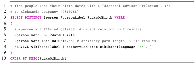
In contrast, the SPARQL Protocol and RDF Query Language (recursive acronym) is a widespread standard to retrieve2 data stored in RDF format. This query language is explicitly designed to make use of the triple structure, where the subject, predicate and object are typically so called uniform resource identifiers (URIs) or literal values (such as strings or numbers). The strength of this approach is that via boolean combination of such atomic queries, results can be retrieved which are not explicitly present in the knowledge base. For example, the simple SPARQL in Listing 1 retrieves a list of persons who have Aleksandr Lyapunov in their “academic lineage”.
| Listing 1. SPARQL Example: “academic lineage” of A. Lyapunov. |
 |
Remark 1.
The relation between an API and a SPARQL endpoint can be summarized as follows: While many objectives can be achieved either by using the API or the SPARQL interface both interfaces are tailored towards different use cases and thus have different strengths and drawbacks.
3. Imperative Knowledge Representation with PyIRK and OCSE
3.1. Imperative versus Declarative Knowledge Representation
Typically, knowledge representation is declarative or passive, e.g., as xml- or rdf-files which need to be interpreted by some program to actually interact with the contained knowledge. This has the advantage to clearly separate the knowledge from the algorithms to process it. However, when developing a new knowledge representation system, this separation has the disadvantage that one needs to co-develop both: the processing code and the representation format. This has to be solved, without a priori knowing specifically what features both components might need, because this would imply to already have some consistent formalization of the domain knowledge available. Furthermore, it poses an additional usability hurdle that potential users or contributors have to familiarize with the representation format (or some adequate interface).
Thus, after some partially successful experiments with declarative approaches, we opted for a different approach which we call imperative representation of knowledge3: It basically means to express the respective knowledge as part of the source code of the knowledge processing software. This is obviously possible since hard-coded strings or variable values are a standard technique in software development. While it is usually a good idea to separate this kind of data from the actual program logic because it might be subject to change independently (e.g., error correction or translation), this can be achieved not only by loading declarative data files but also by suitable modularization of the programming code.
The main advantages of imperative representation of knowledge are, a) that it allows to automate the construction of semantic triples and thus allows for a more compact formulation (in terms of size of the source code) and b) that it spares the user from learning an additional declarative language like, e.g., OWL Manchester syntax (assuming that potential users are familiar with the respective programming language).
3.2. Basic Concepts of PyIRK
As the name “PyIRK” suggests, this framework for imperative representation of knowledge is implemented in the Python programming language. That is, because Python has been proven useful in many applications of science and engineering and thus a high degree of dissemination in the target group can be assumed. Also, the dynamic features of Python (e.g., creating new functions and classes at runtime) support the compact representation of complex knowledge, e.g., evaluated ternary operators such as Lie derivatives.
In Python “everything” (apart from reserved words such as if or for) is an object and thus has a type. The important types (i.e., classes) for PyIRK are Entity (with subclasses Item and Relation), and Statement.
A statement models a branch of the knowledge graph, i.e., a subject-predicate-object triple. Thereby, the predicate is always a reference to a relation, while the subject and object role can be taken by all entities4.
For unambiguous identification of objects in knowledge graphs or ontologies usually one of two paradigms is used: either a) “unique identifier and arbitrary label” (e.g., BFO_0000006 for the class with label `spatial region’ in the Basic Formal Ontology BFO [25]) or b) “unique descriptive label” (e.g., TransferFunctionSystemModel in [5]). While b) is favorable for usability, variant a) clearly has scalability advantages e.g., when modeling concepts which are homonymous i.e., “distribution” or “field” or supporting multiple languages. In PyIRK variant a) is chossen: Every entity has an URI, which specifies the module and the concrete object within that module via a short key I<n> (for items) or R<n> (for relations), where <n> can be replaced by any string consisting of at least one digit. To nevertheless achieve the favorable usability of having consistent labels present in the source code, every entity accepts a valid label as “index”, which is implemented like a dictionary lookup, i.e., using square brackets. Thus, the two lines in Listing 2 are practically5 equivalent PyIRK source code: In both cases the called function istrue receives the exact same arguments and thus return the same value (True). However, the second line has the advantage that the entity references are both precise for a computer and directly understandable for a human.
| Listing 2. Demonstration of “labled identifiers” by two semantically equivalent lines. |
 |
The possibility of using such labeled identifiers enables users to directly understand and create PyIRK source code without the help of additional tools6. This property allows to make use of established technologies and best practises for source code version control. In particular the distributed version control system git is the de-facto standard and repository hosting services such as github, gitlab or codeberg provide useful functionality for collaborative source-code related work such as tracking the change history, parallel branches, merge-requests, and code-reviews. Most importantly this approach makes it easy to create a fork of the whole knowledge base i.e., an independent copy which can be changed and extended without the consent of the original authors7. This “forkability” is important because it prevents the individual control of the knowledge and thus encourages people to experiment with their own fork and eventually exchange contributions.
The approach of representing knowledge as (versioned) software is also consistent with the principle of “continuous provisionality”. This means to accept that the knowledge base will never be complete and that it likely will contain bugs, as it is the case with most complex software systems, but nevertheless might be useful for some task.
3.3. Modules
The knowledge represented in PyIRK is structured in modules. A PyIRK module is a Python file containing source code which, when executed, creates PyIRK entities and statements. Modules can import other modules and collections of closely related modules can be bundled to form a PyIRK package. Such a package consists of at least one module, a configuration file, some documentation and unittests.
3.3.1. Builtin Entities
The most basic module is builtin_entities which is an integral part of the PyIRK framework. It creates abstract items like I1["general item"], I2["Metaclass"], I11["general property"], I12["mathematical object"] and fundamental relations like R1["has label"], R3["is subclass of"], R4["is instance of"], R17["is subproperty of"] etc.
Apart from the mere definition of items and relations it also provides auxiliary Python8 classes and functions such as instance_of. This function creates a new item with generic label (R1) and description (R2) and an R4["is instance of"] statement edge to the provided class (PyIRK item). For example, this allows to create matrix instance, see Listing 3.
| Listing 3. Demonstration of PyIRK instantiation. |
 |
Note that I9904["matrix"] is not defined in builtin_entities but in math1 which is part of the OCSE package (see Section 3.3.2). ¸
3.3.2. Ontology of Control Systems Engineering (OCSE)
Obviously, control theory is not the only field of science for which formal knowledge representation might be worthwhile. It is, therefore, sensible to separate between the PyIRK framework and the actual domain specific content. From the perspective of ontology engineering builtin_entities is an upper level ontology [26], whereas the Ontology of Control Systems Engineering (OCSE) represents a domain ontology.
From a pragmatic perspective the OCSE is just a PyIRK-package containing three different modules:
- agents1: contains humans, institutions and source documents which might be referenced by the other modules. It also contains corresponding relations such as R3474["has ORCID"] and R8439["is described by source"] and auxiliary functions like create_person.
- math1 contains mathematical concepts and relations such as I9904["matrix"], I6709["Lipschitz continuity"], R4963["is neighborhood of"] etc. It also contains auxiliary Python classes like IntegerRangeElement and functions like symbolic_expression_to_graph_expression.
- control_theory1 contains concepts and relations such as I7208["BIBO stability"], I1347["Lie derivative of scalar field"], R5031["has trajectory"], I1664["limit cycle"]. This module is also the place where the Lyapunov-related knowledge is implemented, mostly in form of instances of the builtin items I14["mathematical proposition"] and I20["mathematical definition"], see Section 5.
3.4. Qualifiers
As explained in Section 3.2, basic statements in PyIRK are modeled as triples of the form (subject, predicate, object). For example, using the respective entities from the OCSE module math1 the PyIRK snippet to express that A. Lyapunov worked at National University of Kharkiv is shown in Listing 4. Note that in contrast to natural languages for a semantic triple the predicate does typically not carry any temporal information.
| Listing 4. Single statement without qualifiers. |
 |
Expressing more complex knowledge artifacts by just using triples is not trivial. Wikidata popularized an approach called qualifiers, which consists in introducing a “statement item” for every statement (triple) which should be further described9 and use those as subject for further statements. PyIRK follows a similar approach where Statement-instances (Python objects) are used to serve as nodes in the knowledge graph. Together with some auxiliary functions like start_time and end_time it is possible to make the statement from Listing 4 more precise, see Listing 5.
| Listing 5. Single statement with two qualifiers. |
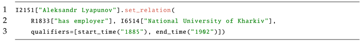 |
Thereby the objects start_time("1885") and end_time("1902") are placeholders which are interpreted by PyIRK such that the appropriate builtin relations R48["has start time"] and R48["has end time"] are used together with the provided literal arguments once the primary statement object has been created.
3.5. Operators and Representation of Formulas
Representation of mathematical knowledge requires to model the application of operators. In PyIRK this is achieved by making those items which have a R4["is instance of"] relation to I4895["mathematical operator"] callable. This allows expressions like I5177["matmul"](A, B) which create new items. In this example snippet a new I9904["matrix"] instance is created, because I5177["matmul"] defines this via R11["has range of result"]. This instance is then related to the operator item via R35["is applied mapping of"] and to the arguments via R36["has argument tuple"] and thus carries all necessary information. Note that operators can have an arbitrary (but fixed) number of arguments.
While this mechanism allows to represent arbitrary mathematical expressions as part of the knowledge graph, it is inconvenient for humans to read and write a formula like with an expression like in Listing 6.
| Listing 6. Formula representation with direct operator calls. |
 |
The flexibility of Python based imperative knowledge representation allows to solve this problem by facilitating the computer algebra package SymPy [30]. In particular the module math1.py defines the functions items_to_symbols and symbolic_expression_to_ graph_expression (short: se_to_ge) to convert between SymPy and PyIRK objects in both directions, see Listing 7. While this requires the a prior definition of the symbols (line 1), the actual representation of the formula is much easier to understand (line 2).
| Listing 7. Formula representation via SymPy |
 |
Remark 2.
It is worth mentioning that SymPy also supports parsing LATEX strings. This offers the possibility to denote formulas in a more widely used syntax if desired.
3.6. Scopes
Many knowledge artifacts (such as theorems or definitions) consist of multiple simpler statements which are in a specific semantic relation to each other. Consider the following version of the well known Pythagorean theorem:
Theorem 1.
Let be the sides of a triangle, ordered from shortest to longest, and the respective lengths. If the angle between a and b is a right angle then the equation holds.
Such a theorem consists of several “semantic parts”, which in the context of PyIRK are called scopes. In particular, we have the three following scopes:
- setting: “Let be the sides of a triangle, ordered from shortest to longest, and (la, lb, lc) the respective lengths.”
- premise: “If the angle between a and b is a right angle”
- assertion: “then the equation holds.”
The concepts “premise” and “assertion” are usually used to refer to parts of theorems and similar artifacts and can be considered self-explanatory. The “setting”-scope is used to refer to those auxiliary statements which “set the stage” to properly formulate the premise and the assertion (e.g., by introducing and specifying the relevant objects). In the literature (formulated in natural language) much of this information is usually provided by the text preceding the actual theorem or by introductory phrases like “Let ...”.
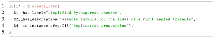
To represent the actual content of a theorem in PyIRK, this theorem has first to be created as item. In Listing 8 we continue the example of the (simplified) Pythagorean theorem for demonstration purposes.
| Listing 8. Creation of the theorem item as implication-instance. |
 |
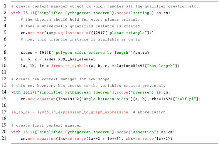
Now, we can create three scope items as instances of I16["scope"], associate them to the theorem item by means of R21["is scope of"] and specify them with R64["has scope type"] as setting, premise, and assertion. These scope items can then be “attached” via a R20["has defining scope"] qualifier to a statement, to express that this statement is not a “top level statement” but instead a part of a theorem structure. For example, a statement which has an R20 qualifier edge to a premise scope is considered to express a condition. In principle all these item- and qualifier-creations could be expressed directly but to provide a more convenient way PyIRK makes use of Python’s context managers – indented code blocks introduced by a with-statement. Listing 9 shows this technique beeing applied to the Pythagorean theorem.
| Listing 9. Specification of the content of the Pythagorean theorem. |
 |
3.7. Rule Based Reasoning
One major advantage of description-logic-based ontologies (represented in OWL) is the availability of so called reasoners or inference engines. These are a pieces of software that are able to infer logical consequences from a set of “facts”, i.e., asserted statements [31]. Additionally to OWL the Semantic Web Rule Language (SWRL) is supported by some reasoners. However, even the expressiveness of both approaches combined is not sufficient for a meaningful representation of mathematical knowledge. For example, while such reasoners can easily infer new statements (edges in the knowledge graph) involving already known entities (nodes in the knowledge graph, “individuals” in OWL-terminology) it is impossible to infer the existence of new entities. A different reasoning approach which overcomes this limitation is known as “existential rules” see, e.g., [32,33].
Being an experimental knowledge representation framework PyIRK implements its own rule based inference engine. It follows the principle that the rules themselves should be part of the overall knowledge graph (instances of I41["semantic rule"]). The content of each rule can be expressed (similar to a mathematical theorem) by means of “setting”, “premise” and “assertion”. Thereby the first two scopes define to which entities (nodes) the rule matches, whereas the third scope defines the consequences of such a match i.e., the creation of new statements or items. Listing 10 shows a simple example which expresses the transitivity of beeing a subproperty: If is subproperty of and is subproperty of , then should also be a subproperty of .
| Listing 10. Definition of a Semantic Rule. |
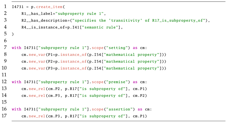 |
In order to apply such a rule, PyIRK uses the VF2 algorithm [34] implemented in the package NetworkX [35] to find so called subgraph monomorphisms. These are subsets of nodes and edges of the overall knowledge graph which match the structure defined by the scopes “setting” and “premise”. For all such subgraph monomorphisms the relations of the scope “assertion” are created (with the respective bindings). For example without applying any rule the property I9642["local exponential stability"] is only a subproperty (R17) of I4900["local asymptotical stability"]. However, after applying rule I4731 from Listing 10 this property is also a subproperty of I2931["local Lyapunov stability"] and Item I5082["local attractiveness"]. As a consequence, it is possible to find systems which have a localy asymptotically stable equilibrium point via a SPARQL search even when searching for the more general property local Lyapunov stability. For a control theory expert this might seem trivial but for users who are not familiar with the subtle relations between different stability concepts this is a significant facilitation.
To implement existential rules, i.e., rules that have new nodes as consequence, PyIRK offers the mechanism of so called “consequent functions” which are attached to an item in assertion scope. They can contain arbitrary code and thus can be used to create new items or relations. A similar mechanism, called “condition function” (attached to an item in premise scope) can be used to improve or simplify the subgraph matching for finding all relevant subgraphs for a given rule.
Remark 3.
In the current development state of PyIRK it is not yet possible to convert the information contained in condition- and consequent-functions into semantic triples when exporting the graph to RDF format. However, implementation is planned as one of the next development steps.
The main applications of semantic rules in PyIRK are a) to derive “new” knowledge and b) to implement measures of quality assurance (see Section 3.8). While it would be possible to implement these types of algorithms directly in the source code of the framework, one must recognize that such algorithms are also relevant knowledge and thus should be a regular part of the overall knowledge graph.
To demonstrate the capabilities (and remaining limitations) of the rule engine a formalized version of “Einsteins zebra riddle” – a famous and comparatively hard logical puzzle attributed to Albert Einstein [36] – is included as part of PyIRK test suite, see [10]10. A logic puzzle was chosen to explain how “new” knowledge is meant: Creating new relations between entities which follow logically from given ones. In other words, the knowledge has already been there, but only in implicit form and thus hard to access, for example, to be used for query-answering.
3.8. Quality Assurance via Type- and Consistency Checking
From our own experience in research and teaching it is obvious that intellectual activity is in principle error prone: texts and formulas contain typos, calculations contain errors, software contains bugs. Mechanisms like careful double checking and peer review can reduce this effect but formal knowledge representation additionally allows for automatic checks (similar to unit tests in software engineering). In particular, PyIRK offers several automated checks:
Firstly, (almost) every11 labeled identifier (cf. Listing 2) in an expression like I38["positive integer"] is checked for consistency against the actual label (R1) of the referenced entity. In this example snippet this is not the case, as the correct label for item I38 would be "non–negative integer". In other words: This mechanism prevents to mistakenly use the wrong items in the modeling process. It is worth mentioning, that this mechanism is compatible with multilinguality of PyIRK. For example, the expression I39["positive Ganzzahl"@de] is valid.
Secondly, due to the inheritance (R3["is subclass of"]) and instantiation R4["is instance of"] it is possible to check the types of relations or operators-items (see Section 3.5) which are applied to other items.
Finally, semantic rules (see Section 3.7) can be used for more specialized consistency checking, e.g., ensuring that only matrices are multiplied with according column and row numbers.
3.9. Modeling Strategy and Implementation State
A mayor challenge in knowledge representation is to define the limits of the domain of discourse or, in other words, to answer the question: “Where to begin?”. This becomes increasingly difficult if the principal ambition of the framework is, like in the case of PyIRK, the capability to consistently represent all relevant scientific knowledge which is traditionally contained in books or articles.
PyIRK approaches this challenge in a pragmatic way: items can be introduced as instances of I50["stub"]12 which indicates that this item is yet incompletely modeled and serves as placeholder. Nevertheless, such stub items can be used in semantic triples with other item and thereby already model valuable knowledge. If deemed necessary the stub items can be modeled more precisely at a later time point, e.g., by introducing other stub-items and thereby pushing the limits “outwards”, away from the more relevant items.
For instance, the example in Listing 9 refers to I2917["planar triangle"]. In a first step this could be introduced as a stub-item. Later, this could be made more precise by introducing a new stub item “planar polygon” and make I2917 a subclass of it. Finally, one might decide to introduce an elaborated taxonomy of geometric objects and integrate triangles and polygons in it. The mayor advantage of the stub-approach is that non-trivial taxonomic modeling effort can be deferred when the current focus is on some concrete problem like representing the lengths of the sides of a triangle.
Having properly set taxonomic relations via R4["is instance of"] and R3["is subclass of"] often is not enough to formally explain what a concept really means. PyIRK handles this challenge by instances of I20["mathematical definition"], which like propositions or rules can have setting, premise and assertion scopes. For example I5325["Hurwitz polynomial"], is first introduced as an instance of I4239["abstract monovariate polynomial"] and then made more precise via I5325["Hurwitz polynomial"].set_relation(p.R37["has definition"], I4455["definition of Hurwitz polynomial"]), where I4455 specifies (via the three scopes) that if the set of roots of that polynomial is a subset of the open left half-plane of then it is a Hurwitz polynomial.
Obviously, this approach is tedious, especially at the beginning but once a “critical mass” of items and relations is accumulated it gets easier as less new entities have to be introduced to express the actual intention, e.g., a new theorem.
At the time of writing the OCSE (version 0.3) and the underlying framework PyIRK (version 0.12) are still under heavy development. When all three OCSE modules are loaded the knowledge graph contains items, of which are automatically created, e.g., scope items, applied operators, etc. Between nodes there exist edges (statements), each of which is specified by one of relations. Additionally there are qualifier statements.
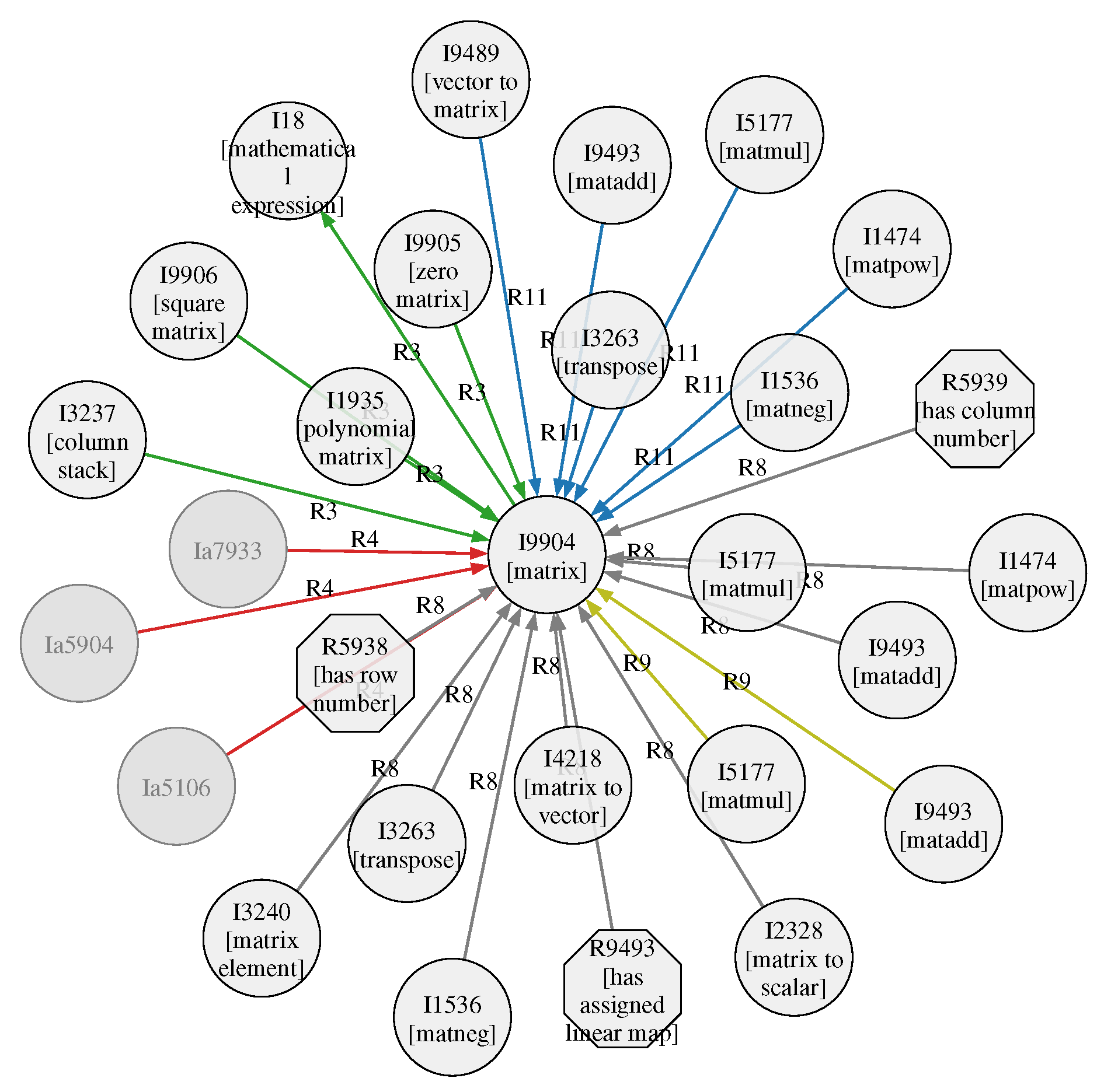
Ironically, despite the resulting data structure being called knowledge graph, a meaningful depiction of the whole data is surprisingly difficult, as Figure 1 demonstrates. A more useful visualization can be achieved when considering only a sub-graph, as e.g., in Figure 2.
In its current development state a PyIRK knowledge graph can be exported to the RDF standard, however, without the qualifier statements. This is not a principal limitation but simply not yet implemented.
The RDF export is the basis for the SPARQL interface, which can be used to perform a semantic search, see Section 6.3. As for other knowledge management systems the full functionality of the framework is only available vial the API, i.e., using the Python library, see also Remark 1.
4. Lyapunov Theory
The study of nonlinear dynamical systems revolves around a number of nonlinear analysis tools. Usually, the stability of a feedback system is of particular interest. One widely used concept for the analysis of nonlinear systems is Lyapunov’s stability theory. This section presents the basic concepts of Lyapunov theory, starting with time-invariant systems.
The following definitions and theorems are based on the extensive descriptions in [37, Sec. 4.1], [38, Sec. 3.4.2] and [39, Chap. 1–3].
4.1. Stability of Equilibrium Points
Consider the nonlinear time-invariant dynamical system
where the map is locally Lipschitz and maps from to . Assume is an equilibrium point of system (1), meaning it satisfies . Without loss of generality, we can assume that the equilibrium point is the origin, .
Definition 1.
The equilibrium point of (1) is called stable (in the sense of Lyapunov), if for any there exists a , such that .
Definition 2.
The equilibrium point of (1) is called asymptotically stable, if it is stable and there exists a , such that .
In order to assess whether an equilibrium point has any of these properties, a criterion is needed. As an inspiration, lets consider a pendulum near its lower equilibrium point. The energy of the system is lowest in its (lower) equilibrium point and increasing in an environment around the equilibrium. Thus, if the energy of the system always decreases along its trajectory, it will eventually reach the equilibrium point.
The same argument holds for other physical systems. One can examine the energy of such systems along its trajectory to evaluate the stability of the equilibrium. Lyapunov showed that this concept can be generalized to specific scalar functions that allow the determination of stability of an equilibrium point, even if energy might not be a meaningful concept for the given system.
We denote with
Theorem 2.
Let be an equilibrium of (1) and an open environment of 0. If there exists a scalar
functionsuch that
- V is positive definite on D,
- is negative semi-definite on D,
is called locally stable (LS). If is even negative definite, is locally asymptotically stable (LAS).
Remark 4.
Technically speaking, the previous Theorem consists of two separate Theorems. Since most of setting is the same, one usually formulates the statement like in Theorem 2. We will recall this fact later in Section 5.
If such a function V exists, it is called Lyapunov function. Additionally, it is called weak/ non-strict, if is negative semi-definite and strong/strict, if is negative definite.
In order to generalize the concept of local asymptotic stability to the global case, one has to make sure, that the definiteness conditions of V hold not just in a neighborhood of the origin, but in the entire state space. Additionally, the Lyapunov function V needs to be radially unbounded.
Definition 3.
Let be an equilibrium of (1). If there exists a scalar function such that
- V is (globally) positive definite,
- is (globally) negative definite,
- (V is radially unbounded),
x* = 0 is called globally asymptotically stable (GAS).
4.2. Construction of Lyapunov Functions
In general, the previous theorems are only sufficient but not necessary, leading to the problem of finding a suitable Lyapunov function for a given system. While there is no general approach to finding a Lyapunov function, there is, however, a number of publications regarding Lyapunov functions for specific systems or under certain conditions.
In the case of the linear system
a candidate for a Lyapunov function is given by the quadratic form
with the positive definite Matrix P. When evaluating the time derivative of along the systems trajectory, one gets
with the symmetric matrix Q. Here
is called Lyapunov equation.
To show that V is indeed a Lyapunov function, we have to prove that the matrix Q is positive definite (see Theorem 2). To satisfy both conditions, one usually starts by choosing a positive definite matrix Q and solves the Lyapunov equation (5) for the matrix P. If P is also positive definite, is indeed a Lyapunov function.
Theorem 2.
Remark 5.
To make the universal quantifier in the previous statement more explicit, one might reformulate the Theorem in short notation
In the case of nonlinear systems, several approaches to construct a Lyapunov function have been discussed (see e.g., [40] for an overview). Most of these methods make assumptions about the system, limiting the applicability of the presented method to a certain class of system.
For demonstration purposes w.r.t. knowledge transfer, our contribution aims at helping to find the suitable method for a given system. To this end, the requirements and assumptions of different approaches are of particular interest to the knowledge representation. Subsequently, we recall two methods of constructing Lyapunov functions with different conditions.
4.2.1. Recursive Algorithm by Vannelli and Vidyasagar [41, Theorem 4]:
This algorithm is applicable to time-invariant systems of dimension two or greater, that can be written as
with homogeneous functions of degree i and under the assumption, that the linearized system
is asymptotically stable. Starting with solving the Lyapunov equation for the linearized system (which has a solution, since the linearized system is stable), a recursive system of equations is defined. Solving these equations leads to a Lyapunov function. For details, see [41, Theorem 4].
4.2.2. Algorithm by Goubault et al. [42]:
This algorithm can be used to examine time-invariant polynomial systems of the form
with an equilibrium in the origin. Now with the use of so called Darboux polynomials, one can search for so called differential variants of the system via so called Sum-Of-Squares programming. If a solution exists, the differential variant can be used to calculate a Lyapunov function. What this means exactly is beyond the scope of this paper. It is only important, that some conditions on the applicability of the algorithm are imposed, that can be represented in our KG.
In the following section, the implementation of some selected theorems in PyIRK will be discussed.
5. Lyapunov-Theory-related Knowledge Representation
As mentioned before (see Section 3.9), a challenge in knowledge representation is where to begin. Therefore, for now, we focused only on implementing the necessary mathematical basics that are needed, to formulate important theorems in the context of Lyapunov theory. That means, that different concepts are implemented in different levels of detail, meaning there will be items with rigorous (mathematical) definitions, items with meaningful (semantic) descriptions and relations and stub items (see Section 3.9). As it becomes necessary, new items or information about an item may be added on demand.
Consider Theorem 2. The Theorem itself is represented by an item defined in the OCSE module control_theory1, see Listing 11.
| Listing 11. Theorem item for Lypunov stability. |
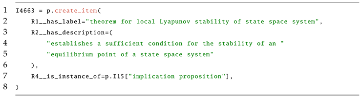 |
This item by itself only has a label (R1), a short description (R2) and the type I15["implication proposition"] (assigned via R4). At this point the item has no relation to any of the concepts in Theorem 2, such as stability. To formally define the content of the theorem and build the corresponding relations in the knowledge graph, we can use the structure of scopes (introduced in Section 3.6), to formulate setting, premise and assertion. To do so, we require the existence of various (mathematical) concepts, such as system, equilibrium point, scalar function, positive definiteness and Lie-derivative to name a few. Some of these concepts need to be specified even more, e.g., the system (meaning system of ordinary differential equations) has to have an associated vector field, to calculate the Lie-derivative and the concept of positive definiteness needs its own definition. Assuming all of the above mentioned items are defined, Theorem 2 can be implemented as shown in Listing 12.
| Listing 12. Theorem for local Lyapunov stability of state space systems. |
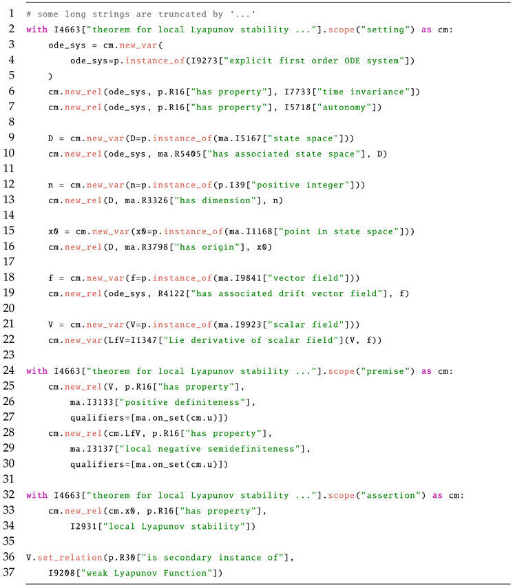 |
Listing 12 mainly consists of three scopes, setting, premise and assertion. In the first scope, the setting, variables are defined that are needed in premise and assertion. Naturally, we start by defining the system of equations (lines 3–5). Since Theorem 2 refers to the autonomous time-invariant system (1), the statement is restricted to systems with these properties by lines 6–7 (even though a similar statement can be made for systems without these properties). The corresponding state space D of the system is defined in l. 9 and is immediately put into relation with its system via l. 10. To specify the dimension of the state space, some positive integer n (l. 13), is put into relation with the state space (l. 14). Next, the origin of the state space (l. 15–16) is defined. As mentioned before, the system described by its drift vector field f, which is defined in l. 18–19. To prepare the discussion of properties of the scalar field V and its derivative in the premise, V and its Lie derivative are formally defined in l. 21–22. Note that =I1347["Lie derivative of scalar field"] is an item of type operator, that takes the two arguments V, f and returns an evaluated mapping (see Section 3.5) of type ma.I9923["scalar field"] (not visible here). This first part of the code corresponds with the first two lines of Theorem 2. Now all required tools are available, to formulate the implication. The premise is rather short. Two conditions need to be fulfilled for the assertion to be true: These definiteness conditions need only hold in the neighborhood of the origin, which we describe by adding a qualifier to the statement, that restricts the statement to the condition of the qualifier. In the assertion, we create a new relation between the origin of the system and the item for local Lyapunov stability (l. 33–34). The last lines 38–40 are not necessarily part of the theorem and take the place of a terminological remark, stating that the functionV is called a weak Lyapunov function.
When adapting this definition for asymptotic stability, we can reuse the setting of Listing 12 via cm.copy_from, see Listing 13:
| Listing 13. Theorem for local asymptotic Lyapunov stability of state space systems. |
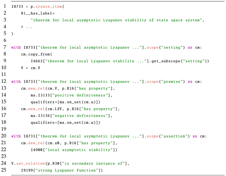 |
Listing 13 copies the setting of the previous theorem. With the slight change of exchanging the item for negative semidefiniteness (ma.I3137) for negative definiteness (ma.I3136), one can formulate the statement for local asymptotic stability.
In a similar fashion, statements regarding the construction of Lyapunov function can be stated. E.g., Theorem 3 reads like this in PyIRK:
| Listing 14. Setting of Theorem 3. |
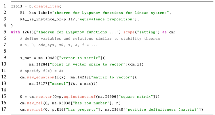 |
Note that this is an equivalence proposition (I17) rather than an implication proposition (I15), meaning that the statement is also true, if premise and assertion are switched. For the sake of brevity, the creation of some items and relations is omitted here. Note further that lines 9–13 feature a number of type conversion operators to ensure type safety during the statement of matrix equations. Lastly, lines 15–17 use the “universally quantified” expression to create the matrix Q, since the premise has to hold for all positive definite matrices Q.
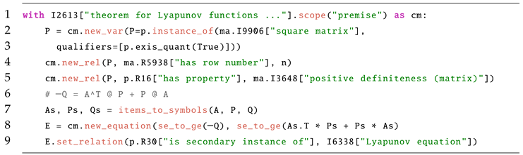
In the premise in Listing 15, a statement about the existence of a specific matrix P is made. Note the existential quantifier in line 3. Afterwards, additional conditions are imposed on the matrix P. Thereby, the SymPy-based formula representation is used, see Section 3.5.
| Listing 15. Premise of Theorem 3. |
 |
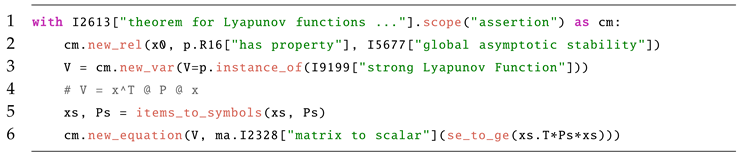
In the assertion (Listing 16) we assign the property of global asymptotic stability to the origin, as well as defining the Lyapunov function V in relation to the matrix P.
| Listing 16. Assertion of Theorem 3. |
 |
Other approaches to finding a suitable Lyapunov function for a given system are implemented in a similar fashion. In particular it is made clear, what the requirements of an approach are and to what kind of system it is applicable to. Steps towards an application of this knowledge are proposed in Section 6.3.
In addition to the aforementioned theorems, many items and relations were implemented in the context of Lyapunov theory (see Appendix A). In total, the OCSE is comprised of items13.
6. Benefits and Applications
With PyIRK and the OCSE, knowledge is formally represented in a way understandable for humans and machines alike. As announced in Section 1 the aim of the current contribution is not to provide a doubtlessly useful product, but instead to present a possible backend for such a knowledge-based application. Nevertheless, the current development state enables some advantages of formal knowledge representation.
6.1. Hierarchies and Dependencies
By explicitly stating the relationships between items and having to explicitly decide the type of every used item or variable in a theorem, the underlying knowledge graph consists of densely connected nodes. This enables the user to infer information about a node (an item) by examining its relations. With the R4["is instance of"] or R3["is subclass of"] relations, a hierarchical structure is imposed on an item. E.g., I5677["global asymptotic stability"] is an instance of I5236["general trajectory property"], which in turn is an instance of the metaclass I54["mathematical property"]. This categorizes the item in a broad way. Additional relations, such as R17["is subproperty of"] relate the item to other items in the graph. In this case, I5677["global asymptotic stability"] is a subproperty of I8744["global Lyapunov stability"], I8059["global attractiveness"] and I4900["local asymptotic stability"]. These relations are transitive, implying that, if the property GAS applies, the property LAS applies as well. Or in other words, if the trajectory is not LAS, it can’t be GAS (see also Section 3.7).
In the context of learning and teaching, the graph of relations between different pieces of information might be helpful to understand, which concepts depend on each other, meaning e.g., what kind of mathematical concepts, such as positive definiteness, are necessary to understand about Lyapunov functions. The careful reader might have noticed, that in the previous code snippets, two different items with the label “positive definiteness” were used (I3133["positive definiteness"] and I3648["positive definiteness (matrix)"]). This is because the concept of a positive definite scalar function differs from the concept of a positive definite matrix, although the two are related.
6.2. Quality Control
Even though written publications are usually proofed multiple times, random mistakes and typos, especially in formulas, might still occur. Such errors might include confounding the vector field and scalar field in a Lie derivative, forgetting a transposition sign on a vector or messing up an index notation. With the information in the OCSE being machine readable, we can automate the process of finding such errors. This can be done by formulating dedicated rules (instances of I47["constraint rule"]), that are part of the knowledge graph itself, see Section 3.7. Currently, three types of mistakes can be caught.
First, mathematical operators such as multiplication and addition, but also Lie derivative and scalar field only should accept arguments of specific types. E.g., the I1347["Lie derivative of scalar field"] takes two arguments of type vector field and scalar field, respectively. An erroneous implementation of , meaning the Lie derivative of a vector field along a scalar field, would result in a raised WrongArgType-error.
The second powerful means for quality control is to make sure, that e.g., the matrix multiplication operator only accepts matrices of adequate size. Keep in mind, that PyIRK does not evaluate any numerical multiplication, but it only stores the operation and its arguments. The quality assurance is thus again done by the suitable rules (see Section 3.7) and can be implemented for all kinds of operators.
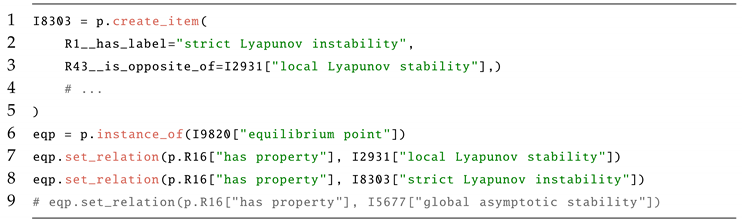
A third tool for quality control is the detection of problematic statements, i.e. incompatible statements or logic errors. An example would be that the same equilibrium point can’t be locally stable and unstable at the same time. An exemplary statement like in Listing 17 would result in an error, since strict Lyapunov instability and local Lyapunov stability have to opposite relation, meaning they cant be true at the same time. Due to the transitivity of property relations, the same error would occur, if line 8 was exchanged for line 9.
| Listing 17. Contradicting statements. |
 |
6.3. Semantic Searchability
With the help of the SPARQL interface (see Section 2.3), we can query the KG for specific information. One might be interested in finding a Lyapunov function for a given system. This can be facilitated, by defining the system and its important properties as part of the KG and then running a SPARQL query to search for theorems that apply to this concrete system. E. g, the system in question could be time-invariant and its differential equations could be polynomial. One would define this system as shown in Listing 18.
| Listing 18. Definition of test system |
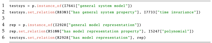 |
Remark 6.
When talking about dynamical systems, one usually attributes certain properties to them. To avoid ambiguity, the OCSE distinguishes between properties of the system, such as time-variance, properties of the mathematical representation of the system, such as linearity and properties of a trajectory of the system, such as local stability.
With the item testsys in the KG, one can use the following SPARQL query (Listing 19) to search for all theorems applicable to this system.
| Listing 19. SPARQL query for applicable theorems |
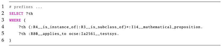 |
Note that ?th matches all items in the KG with the two specified conditions. They have to be of type (instance of subclass(es)) of mathematical proposition, which includes e.g, implication theorems and equivalence propositions, and they have to apply to the system of interest. Consequently the result of the query, shown in Listing 20,¸ consists of the two algorithms that are applicable to time-invariant polynomial systems.
| Listing 20. Result of the SPARQL query |
 |
Analogously, all three algorithms of Section 4.2 will be returned, if the test system was a linear time-invariant system.
The logic behind the relation R80["applies to"] looks at all theorems and makes sure, that conditions expressed in their setting scopes match with the conditions of all the systems in the KG. Each match between theorem and system is connected with the
R80
relation.
Although this is a rather rudimentary example, the SPARQL interface can prove a powerful tool in the future, once the number of theorems and definitions. increases. Note that, this search mechanism is much more powerful than simple text based search.
7. Conclusion and Outlook
In this contribution we present a novel imperative approach for formal representation of control engineering knowledge with the focus on concepts and theorems from Lyapunov theory. We demonstrate that it is possible to model this kind of non-trivial information in a way which enables subsequent applications such as automated quality assurance and enhanced search. Thereby, the basic approach is to exploit the expressive power of a full-featured programming language, as opposed to, e.g., the various OWL profiles which are optimized for reasoning computability and performance at the cost of expressiveness. This facilitates techniques like scopes, applied operators or convenient formulas. Nevertheless, the resulting knowledge graph can be exported to RDF and thus is compatible to the most widespread standard of the semantic web.
The benefits and applications shown (see Section 6) mainly serve as proof of concept. The long-term goal is to develop assistance software, which e.g., helps to find a suitable Lyapunov function for a given dynamical system or to solve other control problems. Such assistant software might improve the accessibility of the large corpus of control-theory and thus facilitate the knowledge transfer between various niches of control engineering, as well as into (new) potential application domains.
In any case, the availability of an open and multilingual domain specific knowledge-repository can be seen as a value by itself, as it helps to communicate progress (and formulate questions) precisely and with little effort (just by issuing a merge-request). The git-based infrastructure greatly supports this usage as it makes it easy to have different (experimental) versions of the knowledge base available (in git branches) and also allows to precisely track every change to the knowledge w.r.t. the author, commit time and commit message.
While this paper shows that formal representation of non-trivial control-engineering content is possible, many questions remain open for future research and development, for example:
- How can contributions to the OCSE (new entities and statements, but also manual quality assurance) be incentivized?
- How exactly can the KG be processed to provide useful information and thus facilitate the desired knowledge transfer?
- How can the computational performance be improved to maintain current loading and reasoning times (some seconds) also when the number of nodes and relations increases by an order of magnitude?
- Is there a relevant educational effect of formalizing knowledge or peer-reviewing formalized knowledge14?
- Assuming that there will be a relevant number of external contributions: How should the plurality of possible perspectives (different concepts, methods, notations, theories) on scientific questions be dealt with?
However, based on the direct feedback we got during the last two years, the biggest open question is how our KG-based approach (i.e., “symbolic AI”) compares to and can be combined with learning based approaches (“numeric AI”) such as LLMs. In the last years, LLM-based systems (such as ChatGPT) have impressively demonstrated both their capabilities as well as their shortcomings. Our expectation is, that the availability of a precise knowledge base such as a KG can be used to overcome the problem of neural-networks-hallucination, or at least to detect it.
Another possible combination is to use an LLM to extract distinct kinds of knowledge directly from selected source files (such as papers) and convert it in PyIRK source code. This could drastically reduce the manual effort necessary for formalizing knowledge. Consequently, this could make it realistic to indeed formalize a significant part of the control engineering knowledge.
Answering the question whether the symbolic (KG) or the numeric (LLM) based approach is better for knowledge representation, will probably be very sensitive on the concrete task and the definition of “better”. In any case a major advantage of the symbolic approach will always be the explainability, i.e., the direct and transparent link between the result and the source data (the knowledge graph).
Abbreviations
The following abbreviations are used in this manuscript:
| MDPI | Multidisciplinary Digital Publishing Institute |
| DOAJ | Directory of open access journals |
| TLA | Three letter acronym |
| LD | linear dichroism |
Appendix A. List of Items and Relations in the Context of Lyapunov Theory
The following list of items, which relate to Lyapunov theory, is implemented in the OCSE.

Table A1.
List of implemented items relating to Lyapunov theory.
| I1347 | Lie derivative of scalar field |
| I6229 | definition of Lie derivative of scalar field |
| I3133 | positive definiteness |
| I3134 | definition of positive definiteness |
| I3135 | positive semidefiniteness |
| I3136 | negative definiteness |
| I8492 | definition of negative definiteness |
| I3137 | negative semidefiniteness |
| I3648 | positive definiteness (matrix) |
| I6117 | definition of positive definiteness (matrix) |
| I5753 | radially unboundedness |
| I5082 | local attractiveness |
| I8059 | global attractiveness |
| I2931 | local Lyapunov stability |
| I8744 | global Lyapunov stability |
| I4900 | local asymptotic stability |
| I5677 | global asymptotic stability |
| I9642 | local exponential stability |
| I5100 | global exponential stability |
| I8303 | strict Lyapunov instability |
| I2933 | Lyapunov Function |
| I9208 | weak Lyapunov Function |
| I9199 | strong Lyapunov Function |
| I5483 | Control Lyapunov Function |
| I3369 | Sontags formula |
| I4663 | theorem for local Lyapunov stability of state space system |
| I8733 | theorem for local asymptotic Lyapunov stability of state space system |
| I2983 | theorem for global asymptotic Lyapunov stability of state space system |
| I3503 | input-to-state stability |
| I6994 | Chetaev instability theorem |
| I3303 | attractor |
| I5106 | repulsor |
| I9875 | region of attraction |
| I9903 | LaSalle’s invariance principle |
| I6338 | Lyapunov equation |
| I3712 | theorem on Lyapunov equation and Stability |
| I4432 | Vannelli recursive algorithm to find Lyapunov function |
| I8142 | theorem by Vannelli for Lyapunov functions for homogeneous systems |
| I4274 | theorem by Goubault for Lyapunov functions for polynomial systems |
| I7006 | Goubault algorithm to find Lyapunov function |
| I2613 | theorem for Lyapunov functions for linear systems |
Note that items with an asterisk live in the math-module. Note further that positive definiteness appears twice, since there are two different properties with this label (relating to positive definite scalar function and positive definite matrix). The detail of information implemented differs for each item. Some items have rigorous definitions, most items are sorted into the existing hierarchy, meaning they have a parent class and some relations to other meaningful items and some small amount of items is implemented as stub-items, with little more information that their label.
| 1 | In Mathematics the problem is known as “one brain barrier”, cf. e.g., [1]. |
| 2 | SPARQL also allows to insert or delete data, but it is mainly used to retrieve information. |
| 3 | This should not be confused with the word group “imperative knowledge” which is in use as a synonym of “procedural knowledge” and refers to knowledge which can be demonstrated by exercise, e.g., by using a specific tool or playing an instrument which might be hard do be expressed using words. The respective counter-term is “descriptive knowledge” for which the synonym “declarative knowledge” is in use and which should also not be confused with the declarative representation of knowledge. |
| 4 | As described in Section 3.4 about so called qualifiers a statement can also be the subject of another statement. |
| 5 | Technically this behavior is achieved by overloading the __get_item__ method of the class Entity. This method checks the label (see Section 3.8) and then returns self, i.e., the object itself. |
| 6 | Of course auxiliary tools e.g., for autocompletion and visualization are very useful but they are not necessary. |
| 7 | Apart from technical measures this is also facilitated by the appropriate OpenSource license (GPLv3+). |
| 8 | As there is also the notion of PyIRK classes, which is a category of PyIRK items, we make the intended meaning explicit, when it is not obvious from the context. |
| 9 | This introduction of the statement item is done by a triple like (subject, predicate, statement-item) where the predicate URI uses a special name space. For details see [29]. |
| 10 | Unfortunately, the relevant code is too long to be included here. |
| 11 | The “magic” item I000 and relation R000 are exceptions to this, because they can be used with an arbitrary label. Their purpose is to allow (temporary) reference to entities which are not yet existing. |
| 12 | This is inspired by Wikipedias practice of stub articles, see https://en.wikipedia.org/wiki/Wikipedia:Stub. |
| 13 | In current development state we have 848 total item, including 55 builtin items, see Section 3.9
|
| 14 | This question is based on the observation, that the formalization process requires a deep understanding of the respective propositions and the related concepts. |
References
- Kohlhase, M. Mathematical knowledge management: transcending the one-brain-barrier with theory graphs.European Mathematical Society (EMS) Newsletter 2014,92, 22–27.
- Berners-Lee, T.; Hendler, J.; Lassila, O. The semantic web. Scientific American 2001, 284, 34–43. [Google Scholar] [CrossRef]
- Patel, A.; Jain, S. Present and future of semantic web technologies: a research statement. International Journal of Computers and Applications 2021, 43, 413–422. [Google Scholar] [CrossRef]
- Dessimoz, C.; Škunca, N., Eds.The Gene Ontology Handbook; Springer New York, 2017.
- Benavides, C.; García, I.; Alaiz, H.; Quesada, L. An ontology-based approach to knowledge representation for Computer-Aided Control System Design.Data & Knowledge Engineering,118, 107–125.
- Knoll, C.; Heedt, R. “Automatic Control Knowledge Repository” – A Computational Approach for Simpler and More Robust Reproducibility of Results in Control Theory. In Proceedings of the 24th International Conference on System Theory, Control and Computing (ICSTCC); 2020; pp. 130–136. [Google Scholar] [CrossRef]
- Knoll, C. Examining the ORKG towards Representation of Control Theoretic Knowledge–Preliminary Experiences and Conclusions. In Proceedings of the Companion Proceedings of the Web Conference, 2022, pp. 810–817.
- Fiedler, J.; Gerwien, M.; Knoll, C. A Hybrid Tactical Decision-Making Approach in Automated Driving Combining Knowledge-Based Systems and Reinforcement Learning. In Proceedings of the 2022 IEEE 25th International Conference on Intelligent Transportation Systems (ITSC); 2022; pp. 3478–3483. [Google Scholar] [CrossRef]
- Heedt, R.; Knoll, C.; Röbenack, K. Formal Semantic Representation of Methods in Automatic Control. In Proceedings of the Tagungsband VDI Mechatroniktagung, 2021, p. xx. (in German).
- Knoll, C.; Fiedler, J. Python-based Imperative Knowledge Representation (PyIRK) –- Source Repository on GitHub, 2023. https://github.com/ackrep-org/pyirk-core.
- Knoll, C.; Fiedler, J. Ontology of Control Systems Engineering (OCSE) –- Source Repository on GitHub, 2023. https://github.com/ackrep-org/ocse.
- Knoll, C.; Röbenack, K. On configuration flatness of linear mechanical systems. In Proceedings of the 2014 European Control Conference (ECC); 2014; pp. 1416–1421. [Google Scholar] [CrossRef]
- Röbenack, K.; Palis, S. Set-Point Control of a Spatially Distributed Buck Converter. Algorithms 2023, 16, 55. [Google Scholar] [CrossRef]
- Naveed, H.; Khan, A.U.; Qiu, S.; Saqib, M.; Anwar, S.; Usman, M.; Akhtar, N.; Barnes, N.; Mian, A. A Comprehensive Overview of Large Language Models, 2023, [arXiv:cs.CL/2307.06435].
- Guarino, N.; Oberle, D.; Staab, S. What is an ontology? InHandbook on ontologies; Springer Berlin, 2009; pp. 1–17.
- Bergman, M.K.Knowledge Representation Practionary; Springer, 2018.
- Keet, M.An introduction to ontology engineering, v1.5; College Publications, 2020.
- Allemang, D.; Hendler, J.; Gandon, F. Semantic Web for the Working Ontologist: Effective Modeling for Linked Data, RDFS, and OWL, 3 ed.; Vol. 33, Association for Computing Machinery: New York, NY, USA, 2020. [Google Scholar]
- Pease, A.; Niles, I. IEEE standard upper ontology: a progress report. The Knowledge Engineering Review 2002, 17, 65–70. [Google Scholar] [CrossRef]
- Baader, F.; Calvanese, D.; McGuinness, D.; Patel-Schneider, P.; Nardi, D.; et al.The description logic handbook: Theory, implementation and applications; Cambridge university press, 2003.
- Krötzsch, M.; Marx, M.; Ozaki, A.; Thost, V. Attributed description logics: Ontologies for knowledge graphs. In Proceedings of the International Semantic Web Conference. Springer; 2017; pp. 418–435. [Google Scholar]
- Vrandečić, D.; Krötzsch, M. Wikidata: a free collaborative knowledgebase. Communications of the ACM 2014, 57, 78–85. [Google Scholar] [CrossRef]
- Jaradeh, M.Y.; Oelen, A.; Farfar, K.E.; Prinz, M.; D’Souza, J.; Kismihók, G.; Stocker, M.; Auer, S. Open research knowledge graph: next generation infrastructure for semantic scholarly knowledge. In Proceedings of the Proceedings of the 10th International Conference on Knowledge Capture; 2019; pp. 243–246. [Google Scholar]
- Auer, S.; Stocker, M.; Vogt, L.; Fraumann, G.; Garatzogianni, A. Orkg: Facilitating the transfer of research results with the open research knowledge graph 2021.
- Arp, R.; Smith, B.; Spear, A.D.Building ontologies with basic formal ontology; Mit Press, 2015.
- Munn, K.; Smith, B., Eds. Applied Ontology – An Introduction; De Gruyter: Berlin, Boston, 2008. [CrossRef]
- Knoll, C.; Heedt, R. Tool-based Support for the FAIR Principles for Control Theoretic Results: The “Automatic Control Knowledge Repository”.System Theory, Control and Computing Journal 2021, pp. 56–67.
- Fiedler, J.; Knoll, C. Catalog of Dynamical System Models with Semantic Metadata.PAMM 2023,23, e202300049, [https://onlinelibrary.wiley.com/doi/pdf/10.1002/pamm.202300049]. https://doi.org/https://doi.org/10.1002/pamm.202300049. [CrossRef]
- Wikibooks. SPARQL/WIKIDATA Qualifiers, References and Ranks — Wikibooks, The Free Textbook Project, 2021. [Online; accessed 14-December-2023].
- Meurer, A.; Smith, C.P.; Paprocki, M.; Čertík, O.; Kirpichev, S.B.; Rocklin, M.; Kumar, A.; Ivanov, S.; Moore, J.K.; Singh, S.; et al. SymPy: symbolic computing in Python. PeerJ Computer Science 2017, 3, e103. [Google Scholar] [CrossRef]
- Lamy, J.B. Owlready: Ontology-oriented programming in Python with automatic classification and high level constructs for biomedical ontologies. Artificial intelligence in medicine 2017, 80, 11–28. [Google Scholar] [CrossRef] [PubMed]
- Carral, D.; Dragoste, I.; González, L.; Jacobs, C.; Krötzsch, M.; Urbani, J. Vlog: A rule engine for knowledge graphs. In Proceedings of the The Semantic Web–ISWC 2019: 18th International Semantic Web Conference, Auckland, New Zealand, October 26–30, 2019, Proceedings, Part II 18. Springer, 2019, pp. 19–35.
- Ivliev, A.; Ellmauthaler, S.; Gerlach, L.; Marx, M.; Meißner, M.; Meusel, S.; Krötzsch, M. Nemo: First Glimpse of a New Rule Engine. In Proceedings of the Proceedings 39th International Conference on Logic Programming (ICLP 2023); Pontelli, E.; Costantini, S.; Dodaro, C.; Gaggl, S.; Calegari, R.; Garcez, A.D.; Fabiano, F.; Mileo, A.; Russo, A.; Toni, F., Eds., September 2023, Vol. 385,EPTCS, pp. 333–335. [CrossRef]
- Cordella, L.P.; Foggia, P.; Sansone, C.; Vento, M. A (sub) graph isomorphism algorithm for matching large graphs. IEEE transactions on pattern analysis and machine intelligence 2004, 26, 1367–1372. [Google Scholar] [CrossRef] [PubMed]
- Hagberg, A.; Schult, D.; Swart, P. Exploring network structure, dynamics, and function using NetworkX. In Proceedings of the Proceedings of the 7th Python in Science Conference (SciPy2008, Pasadena, CA, USA); 2008; pp. 11–15. [Google Scholar]
- Wikipedia contributors. Zebra Puzzle — Wikipedia, The Free Encyclopedia, 2023. [Online; accessed 27-December-2023].
- Khalil, H.Nonlinear Control Global Edition; Pearson Deutschland, 2014; p. 400.
- Slotine, J.J.E.; Li, W.; et al.Applied nonlinear control; Vol. 199, Prentice hall Englewood Cliffs, NJ, 1991.
- Adamy, J. Nonlinear Systems and Controls; Springer Berlin Heidelberg: Berlin, Heidelberg, 2022. [Google Scholar] [CrossRef]
- Giesl, P.; Hafstein, S. Review on computational methods for Lyapunov functions.Discrete and Continuous Dynamical Systems-B 2015,20, 2291–2331.
- Vannelli, A.; Vidyasagar, M. Maximal Lyapunov functions and domains of attraction for autonomous nonlinear systems. Automatica 1985, 21, 69–80. [Google Scholar] [CrossRef]
- Goubault, E.; Jourdan, J.H.; Putot, S.; Sankaranarayanan, S. Finding non-polynomial positive invariants and Lyapunov functions for polynomial systems through Darboux polynomials. In Proceedings of the 2014 American Control Conference. IEEE, 2014, pp. 3571–3578.
Figure 1.
Visualization of the whole knowledge graph. While it is impossible to extract meaningful details from this picture it illustrates the high degree of interconnection. Edges of type R3["is subclass of"] are blue, R4["is instance of"] are orange and all other edges types are colored black.
Figure 1.
Visualization of the whole knowledge graph. While it is impossible to extract meaningful details from this picture it illustrates the high degree of interconnection. Edges of type R3["is subclass of"] are blue, R4["is instance of"] are orange and all other edges types are colored black.
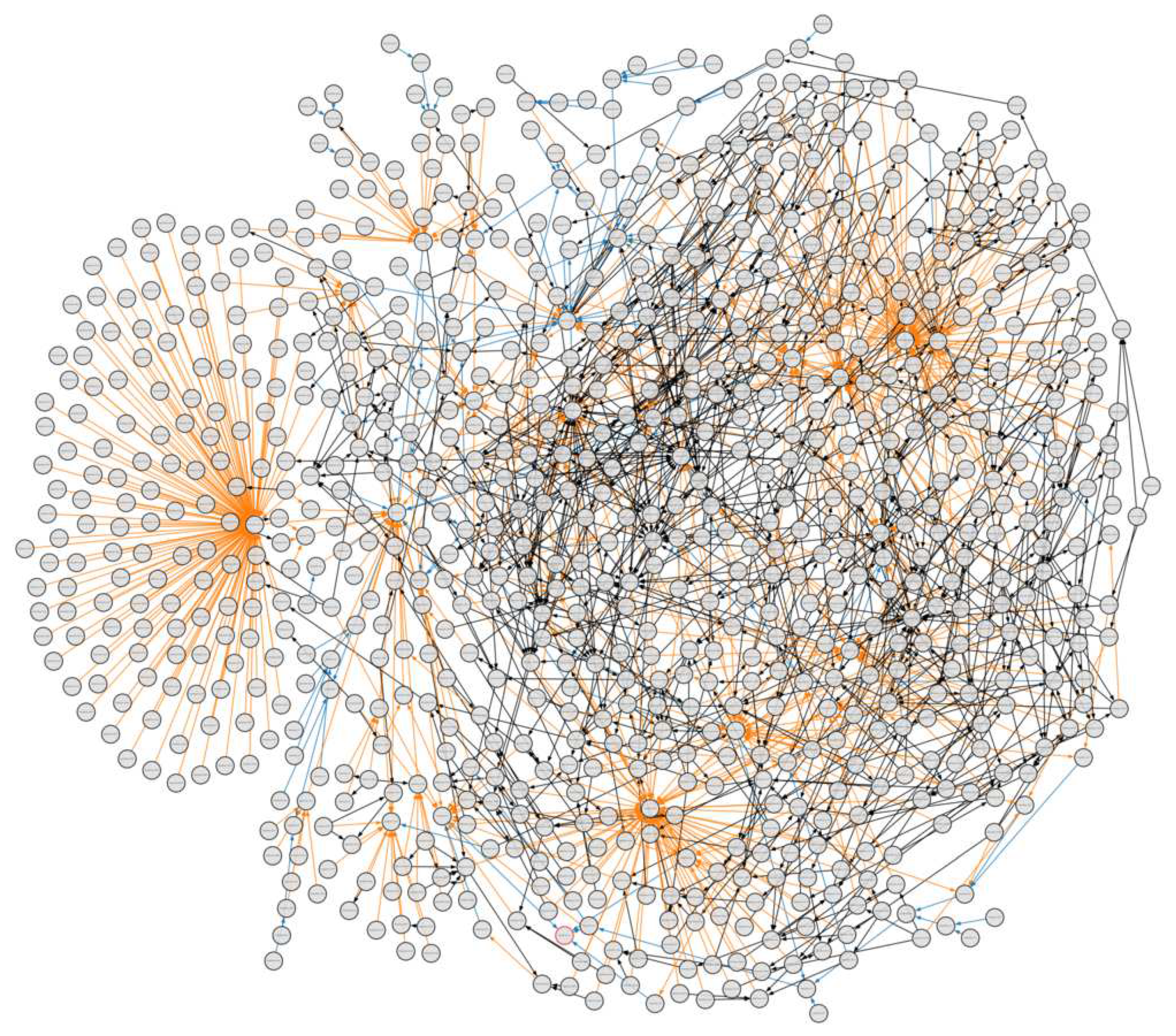
Figure 2.
Visualization of a sub-graph with I9904["matrix"] as the center and only direct neighbors. For the sake of displayability only some of the automatically created instance items (key starting with Ia... are displayed.)
Figure 2.
Visualization of a sub-graph with I9904["matrix"] as the center and only direct neighbors. For the sake of displayability only some of the automatically created instance items (key starting with Ia... are displayed.)
Disclaimer/Publisher’s Note: The statements, opinions and data contained in all publications are solely those of the individual author(s) and contributor(s) and not of MDPI and/or the editor(s). MDPI and/or the editor(s) disclaim responsibility for any injury to people or property resulting from any ideas, methods, instructions or products referred to in the content. |
© 2024 by the authors. Licensee MDPI, Basel, Switzerland. This article is an open access article distributed under the terms and conditions of the Creative Commons Attribution (CC BY) license (http://creativecommons.org/licenses/by/4.0/).
Copyright: This open access article is published under a Creative Commons CC BY 4.0 license, which permit the free download, distribution, and reuse, provided that the author and preprint are cited in any reuse.


