Preprint

Article

EMS for Active and Reactive Power Management in a Polygenerative Microgrid feeding a PED

Altmetrics

Downloads

Views

Comments

A peer-reviewed article of this preprint also exists.

This version is not peer-reviewed

Submitted:

28 December 2023

Posted:

29 December 2023

You are already at the latest version

Alerts

Abstract

Energy management systems (EMS) play a central role in improving the performance of microgrids by ensuring their efficient operation while minimizing operational costs and environmental impacts. This paper presents a comprehensive study of a MILP-based EMS developed and implemented in MATLAB using Yalmip software for the energy management of a new positive energy district in the city of Savona, Italy, as part of the Interreg Alpine Space Project ALPGRIDS. The main objective of this research is to optimize the functioning of the microgrid, focusing on cost efficiency and environmental sustainability. In pursuit of this objective, the EMS undergoes comprehensive testing and analysis, replicating actual conditions and addressing the diverse demands of end-users across typical days throughout the year considering real electricity selling and purchase price. The EMS also accounts for the reactive power capabilities of the various technologies integrated into the microgrid. The levelized cost of electricity (LCOE) serves as a metric for assessing curtailment costs, while penalties related to reactive power absorption from the distribution network are appraised in alignment with prevailing regulatory guidelines. The case study provides valuable insights into the practical implementation of EMS technology in microgrids and demonstrates its potential for sustainable energy management in complex urban energy districts. The insights and strategies developed through this research contribute to the overall goals of improving energy efficiency and reducing the environmental footprint of future energy districts.

Keywords:

Subject: Engineering - Electrical and Electronic Engineering

1. Introduction

In the dynamic landscape of 2021, renewable energy faced several complex challenges due to the ongoing impact of the COVID-19 pandemic, economic volatility and geopolitical tensions. The impact of the pandemic and the rise in commodity prices have disrupted renewable energy supply chains and led to delays in projects. However, amidst these challenges, the discussion on the role of renewables in improving energy security gained momentum, fuelled by a sharp rise in energy prices. Despite these hurdles, the renewable energy sector exhibited robust growth, reaching record highs in power capacity. Investment in renewable power and fuels saw a fourth consecutive year of increase, resulting in solar and wind power jointly contributing over 10% to the world’s electricity generation for the first time [1].

In 2021, the International Energy Agency’s Net Zero by 2050 scenario set ambitious targets, influencing 17 countries’ pledges for net-zero emissions by COP26. The Glasgow Climate Pact emphasized reducing fossil fuel usage, with 140 countries committing to "phasing down" coal power. Notable exceptions like Australia, China, India, and the U.S. did not join in stopping financing for new coal plants.

The renewable energy sector progressed, with a 17% surge in capacity additions in 2021, reaching 314 GW. Global renewable capacity rose to 3,146 GW, but urgent deployment is needed to meet IEA and IRENA benchmarks, requiring 825 GW annually until 2050. With increasing energy demand, microgrids play a pivotal role in the future energy landscape. They offer decentralized and resilient solutions, aligning with global sustainability goals. To address energy wastage, optimize existing microgrids, and transform grids into smart grids, "Smart Microgrids" link users to production systems, balancing supply and consumption in real time. Collaborating with energy communities, microgrids create virtuous urban districts using renewable self-production. Microgrids usually consist of low-voltage distribution networks with distributed energy resources, operating in islanded mode or connected to the main grid [1,2,3,4,5,6,7,12]. Intelligent microgrids enable the minimization of energy exchange with the external grid. It is important to mention that Districts, where annual self-production surpasses consumption on a global scale, are referred to as "Positive Energy Districts" (PEDs) [9].

Microgrids (MGs) face several challenges, including the high investment costs associated with Renewable Energy Sources (RES), the need for optimal energy source utilization, control complexities, a lack of system protection and regulatory standards, and concerns related to customer privacy. Given the prevalent deployment of inherently intermittent RESs and the growing integration of probabilistic controllable loads into MGs, researchers have concentrated on addressing energy management issues.

1.1. Fundamentals, Evolution, and Classification of Energy Management Systems

The International Electrotechnical Commission, through its standard IEC 61970, which pertains to the EMS application program interface in power systems management, defines an Energy Management System (EMS) as "a computer system that comprises a software platform providing fundamental support services and a suite of applications delivering the necessary functionality for the effective operation of electrical generation and transmission facilities, ensuring sufficient security of energy supply at minimal cost" [10]. Similarly, an MG EMS, encompassing these attributes, typically consists of modules designed to execute decision-making strategies. Modules such as DERs/load forecasting, Human Machine Interfaces (HMI), and supervisory control and data acquisition (SCADA), among others, play a crucial role in ensuring the efficient implementation of EMS decision-making strategies by transmitting optimal decisions to each generation, storage, and load unit [11]. Leveraging energy from RES has become standard for enhancing grid resilience and achieving emission reduction goals. As energy demand rises, ensuring a reliable supply is crucial. However, integrating RES presents challenges, necessitating the storage of excess energy, notably in grid-connected Battery Energy Storage Systems (BESS). The sustainability and reliability of grids face hurdles with RES integration, emphasizing the pivotal role of grid-connected BESS in managing surplus energy. In microgrids, whether grid-connected or islanded, effective power flow management is critical. This is particularly crucial given the unpredictable nature of RES, characterized by intermittency and varying availability. To enhance the reliability of microgrids, the integration of BESS is crucial. However, this integration introduces complexity, prompting the need for an EMS to orchestrate and optimize the whole energy system. The EMS acts as the operational brain, ensuring the efficient and effective functioning of microgrids in the face of dynamic and unpredictable energy inputs from renewable sources.

In recent times [26], there has been a substantial upswing in the adoption of large-scale energy storage systems. This surge is propelled by advancements in both the cost-efficiency and performance of energy storage technologies. Furthermore, the necessity to integrate distributed generation, alongside government incentives and mandates, has significantly contributed to this growth. To harness the full potential of energy storage as a flexible grid asset capable of delivering multiple grid services, the implementation of EMSs and optimization methods is imperative. These systems must exhibit adaptability to a spectrum of use cases and regulatory landscapes, ensuring their efficacy and safe utilization in diverse energy storage scenarios.

Energy management strategy can be applied to either grid-connected or islanded microgrids comprising RES and BESS. The optimization can be focused on either cost optimization or minimizing the cash flow of the system as well as power exchange with the main grid in grid-connected mode or in the case of islanded mode to minimize the operation cost and to reduce emissions by scheduling DER in a microgrid [13]. The Energy Management System (EMS) of an MG encompasses both supply and demand-side management, aiming to satisfy system constraints and achieve economical, sustainable, and reliable MG operation [10]. The EMS offers numerous advantages, ranging from efficient generation dispatch and energy savings to reactive power support and frequency regulation. It contributes to enhancing reliability, reducing loss costs, maintaining energy balance, lowering greenhouse gas (GHG) emissions, and fostering customer participation while respecting customer privacy.

EMS with a classical approach as described in [14] is one way to effectively model and manage the MG. The microgrid energy management described here is formulated as a unit commitment problem about the distribution network and the corresponding constraints leading to a mixed-integer non-linear programming (MINLP) formulation to reduce the computational time, the distribution power flow equations and nonlinear constraints are simplified by linearizing the MINLP formulation to mixed-integer linear programming (MILP).

This paper aims to decribes the MILP-based EMS designed for the effective control of active and reactive power in a microgrid intended for integration into the SPEED2030 (Savona Positive Energy & Environment District). This district is envisioned as an extension of the existing University Savona Campus in Italy. The document is structured as follows: Section II accentuates the distinctive features of PEDs and provides an overview of the ALPGRIDS project. Section III outlines the proposed microgrid by detailing the employed technologies and the EMS model its main constraints, the architecture of the optimization model, and the objective function related to it. The input data is briefly outlined in Section IV, presenting its key inputs and assumptions. Section V presents the primary outcomes of EMS and the results, and Section VI concludes the paper.

2. PED and Alpgrids Project

2.1. Positive Energy Districts (PED)

In the last decade, the concept of PEDs has garnered increasing attention as a typical approach to reducing CO2 emissions globally. PEDs are recognized as effective tools for emission reduction in Europe and other parts of the world [15]. Scientific projects and regulatory bodies are actively investigating PEDs to encourage the use of renewable energy sources, reduce GHG emissions, enhance energy flexibility in buildings, and improve overall user comfort [16,17].

A PED is an energy-efficient urban district achieving zero net greenhouse gas emissions through active management of bidirectional energy flows and annual surplus energy generation [15,18]. PEDs, comprised of interconnected buildings linked to the power grid, employ various energy management techniques such as balancing, peak shaving, and demand response. These districts aim to create integrated environments fostering sustainable production, consumption, and mobility, reducing primary energy use and greenhouse gas emissions while providing added value and incentives for consumers.

Aligned with the European Strategic Energy Technology Plan, the ’Positive Energy Districts and Neighborhoods for Sustainable Urban Development’ program, supported by 20 EU Member States and part of JPI Urban Europe [19], strives to establish 100 positive energy neighborhoods by 2025. Engaging diverse stakeholders, including investors, cities, industry players, research organizations, consortia, and private citizens, this initiative aims to contribute significantly to sustainable urban development.

In Italy, several PED projects are already in the planning and development stages across various cities, such as Parma, Milan, Bolzano, Florence, and Lecce [20]. These projects contribute to the broader European effort to advance sustainable urban development and exemplify Italy’s commitment to the goals outlined in the Positive Energy Districts program.

As part of the Interreg Alpine Space ALPGRIDS project [21], an assessment has been conducted to explore the potential of configuring the Savona pilot site as a PED.

2.2. Alpgrids Project

In the Legino district, situated approximately two kilometers from Savona, the ALPGRIDS initiative took root as an extension of the visionary Savona campus.Today, the Savona campus stands as a bustling center for educational institutions, university research laboratories, research centers, and small to medium-sized enterprises [22]. The Savona campus has focused on the ”Energy 2020” project [23], emphasizing sustainable energy principles. Key outcomes include the Smart Polygeneration Microgrid (SPM) and Smart Energy Building (SEB), designed for cost reduction, emissions control, and a comfortable environment [25].

Since 2019, the University of Genoa and IRE Liguria [24] have actively participated in the ALPGRIDS project across five Alpine arc countries. The initiative aims to establish smart microgrids for energy communities through seven pilot projects, including the creation of the urban PED SPEED2030 next to the Savona campus in Legino.

Aligned with PED guidelines [19,20], the Savona ALPGRIDS initiative emphasizes maximizing renewable energy production and optimizing resource utilization at a regional level. Utilizing microgrid configurations and promoting energy sharing through Renewable Energy communities(REC), surplus energy benefits nearby areas, fostering the growth of existing PEDs and inspiring new ones. This approach attracts investments, modernizes infrastructure, and enhances public services [19,20,22].

The available areas for the new Pilot Project areas (SPEED2030) are highlighted in Figure 1 The district is conceptually divided into four zones devoted to different final uses:

The main football stadium, an outdoor sports area, and the swimming pool;
Commercial activity areas;
University labs, research centers and student accommodation;
Social housing.

The pilot site study centered on meeting the stringent supply reliability needs of research laboratories while addressing diverse energy demands, including electricity, heating, and cooling for various buildings. The primary goal was to reduce primary energy consumption and environmental impact. This paper delves specifically into an in-depth analysis of the EMS applied to active and reactive power management within one of the two proposed microgrids for the SPEED2030 project, focusing on a university building within the PED context.

The microgrid is thoroughly investigated, exploring different scenarios that involve both the incorporation and exclusion of the electric mobility component. This comprehensive analysis extends to typical days during both winter and summer seasons. The study aims to assess the microgrid’s performance and resilience under diverse conditions, considering the specific challenges and opportunities posed by electric mobility integration across various seasonal contexts.

3. EMS: Application and Mathematical Model

3.1. Structure and Elements of the Microgrid

The design of the microgrid envisioned for the University’s upcoming structures in SPEED 2030 is illustrated in Figure 2. This AC microgrid incorporates a range of resources, including a Combined Heat and Power (CHP) unit, rooftop-installed Photovoltaic (PV) plants, a micro wind turbine, a chiller, a heat pump, storage battery systems, and Electric Vehicle (EV) charging stations (comprising 2 AC, 2 DC, and 2 V2G types). The model utilized for this configuration is succinctly outlined in the following sections.

The microgrid comprises seven buses, each serving a specific role within the system. Bus 1 functions as the Point of Connection (POC) with the grid, facilitating external connectivity. Bus 2 serves as a coupling bus, completing the ring configuration and enhancing the overall stability of the microgrid. Bus 3 is dedicated to the Microgrid Control Center (MCC) building, a centralized control hub housing the control room. This central control facility is intricately linked with the CHP unit, the chiller, and the rooftop PV installations. Bus 4 is designated as the wind station, managing the integration and utilization of power generated by the micro wind turbine. Bus 5 operates as a BESS station, featuring rooftop PV installations for energy generation. Bus 6 serves as a charging station equipped with PV installations positioned over a shed, emphasizing sustainable energy practices in electric vehicle charging. Finally, Bus 7 is associated with the students accommodation building. This building incorporates rooftop PV installations for power generation and employs a heat pump to address cooling or heating requirements.

This diverse bus configuration illustrates the strategic allocation of roles and resources within the microgrid, showcasing a comprehensive and efficient design for meeting the energy needs of the University’s new buildings in the SPEED 2030 project.

3.2. Mathematical Model

3.2.1. Distributed Generation Model

The distributed generation units in the microgrid consist of three types: PV, wind turbine, and CHP. PV and wind are categorized as non-dispatchable Distributed Energy Resources (DERs), implying their generation is dependent on environmental conditions and not controllable. On the other hand, CHP is considered a dispatchable DER, allowing for controlled and scheduled power generation to meet specific demand requirements.

Renewable Energy Source (RES) Model

In our model, we consider the contribution of RES to the microgrid system. The active power output of the RES at different buses is denoted as $P_{b, r, t}^{RES}$ in kilowatts [kW] as in (1). Additionally, the active power curtailment of the RES is represented by $P_{b, r, t}^{RES, curt}$ in [kW] as in (2), reflecting any reduction in the output due to operational or grid constraints. $P_{b, r, t}^{RES, av}$ represents the available power of RES as in (3). The equation (4) limits the maximum power of RES according to (CEI 0-16 page-117).

The main constraints for RES are as follows:

$P_{b, r, t}^{RES, av} = P_{b, r, t}^{RES} + P_{b, r, t}^{RES, curt}, \forall b = 1 . . B, \forall r = 1 . . R, \forall t = 1 . . T$

(1)

$0 \leq P_{b, r, t}^{RES, curt} \leq P_{b, r, t}^{RES, av}, \forall b = 1 . . B, \forall r = 1 . . R, \forall t = 1 . . T$

(2)

$0 \leq P_{b, r, t}^{RES} \leq P_{b, r, t}^{RES, av}, \forall b = 1 . . B, \forall r = 1 . . R, \forall t = 1 . . T$

(3)

$0 \leq P_{b, r, t}^{RES} \leq A_{b, r}^{RES} cos ϕ, \forall b = 1 . . B, \forall r = 1 . . R, \forall t = 1 . . T$

(4)

For the reactive power, $Q_{b, r, t}^{RES, out}$ in (5) represents the reactive power injected into the microgrid by the RES in [kVAR], while in (6) $Q_{b, r, t}^{RES, in}$ represents the reactive power absorbed by the RES in [kVAR]. $ψ_{r}$ in (5) and (6) limits the inverter operating points considering the rectangular capability curve. Binary variables in (7) $y_{b, r, t}^{RES, out}$ and $y_{b, r, t}^{RES, in}$ take the value 1 when the RES injects or absorbs reactive power, respectively.

The reactive power constraints are given as follows:

$0 \leq Q_{b, r, t}^{RES, out} \leq A_{b, r}^{RES} ψ_{r} y_{b, r, t}^{RES, out}, \forall b = 1 . . B, \forall r = 1 . . R, \forall t = 1 . . T$

(5)

$0 \leq Q_{b, r, t}^{RES, in} \leq A_{b}^{RES} ψ_{r} y_{b, r, t}^{RES, in}, \forall b = 1 . . B, \forall r = 1 . . R, \forall t = 1 . . T$

(6)

$y_{b, r, t}^{RES, out} + y_{b, r, t}^{RES, in} \leq 1, \forall b = 1 . . B, \forall r = 1 . . R, \forall t = 1 . . T$

(7)

These variables play a crucial role in capturing the dynamic behaviour and impact of RES on the microgrid, enabling an analysis of active and reactive power interactions, as well as the ability to curtail power output when necessary.
CHP Model

The electric power produced is subject to the following constraints:

$P_{b, t}^{e l, C H P} \geq P_{b, t}^{e l, C H P, \min} \cdot x_{b, t}^{C H P}, \forall b = 1 \dots B, \forall t = 1 \dots T$

(8)

$P_{b, t}^{e l, C H P} \leq P_{b, t}^{e l, C H P, \max} \cdot x_{b, t}^{C H P}, \forall b = 1 \dots B, \forall t = 1 \dots T$

(9)

These constraints in (8) and (9)limit the power between a lower threshold ( $P_{b, t}^{e l, C H P, \min}$ ) and an upper one ( $P_{b, t}^{e l, C H P, ″ \max ″}$ ). Specifically, $P_{t}^{e l, C H P, \min}$ represents the minimum technical part-load of the microturbine, typically advised by manufacturers to be above 30%-50% of the nominal electrical power to maintain efficiency. Regarding the maximum power $P_{b, t}^{e l, C H P, \max}$ , it depends on the time instant t since the maximum electric power and efficiency are influenced by environmental (temperature, pressure, and humidity) and installation (altitude) conditions.

The thermal power $P_{b, t}^{t h, C H P}$ produced by the single unit at time t can either be positive or equal to zero and is correlated with the electric power $P_{b, t}^{e l, C H P}$ through a linear function as in (10) describing the partial load behavior of the microturbine:

$P_{b, t}^{t h, C H P} \leq \frac{P_{b, t}^{e l, C H P}}{P_{b, t}^{e l, C H P, ″ \max ″}} \cdot P_{b, t}^{t h, C H P, ″ \max ″}, \forall b = 1 \dots B, \forall t = 1 \dots T$

(10)

The primary power of the microturbine $P_{b, t}^{f, C H P}$ at time t is linearly related to the electric power produced $P_{b, t}^{e l, C H P}$ through equation (11):

$P_{b, t}^{f, C H P} = P_{b, t}^{f, C H P, ″ \max ″} (α_{b}^{f, C H P} \cdot \frac{P_{b, t}^{e l, C H P}}{P_{b, t}^{e l, C H P, ″ \max ″}} + β_{b}^{f, C H P}), \forall b = 1 \dots B, \forall t = 1 \dots T$

(11)

where $α_{b}^{f, CHP}$ and $β_{b}^{f, CHP}$ are constant coefficients. Finally, in the following equation (12) thermal balance is defined:

$P_{b, t}^{th, CHP, heating} + P_{b, t}^{th, CHP, chiller} = P_{b, t}^{CHP}$

(12)

where $P_{b, t}^{th, CHP, heating}$ and $P_{b, t}^{th, CHP, chiller}$ can assume positive values or be equal to zero.

$P_{b, t}^{th, CHP, heating} \geq 0, \forall b = 1 \dots B, \forall t = 1 \dots T$

(13)

$P_{b, t}^{th, CHP, chiller} \geq 0, \forall b = 1 \dots B, \forall t = 1 \dots T$

(14)

For the reactive power, the equations (15) and (16) are given below which considers the rectangular capability curve and the binary variable in (17) takes the value 1 if the CHP is producing reactive power or 0 if absorbing the reactive power respectively:

$0 \leq Q_{b, t}^{CHP, out} \leq A_{b}^{CHP} \cdot y_{b, t}^{CHP, out}, \forall b = 1 \dots B, \forall t = 1 \dots T$

(15)

$0 \leq Q_{b, t}^{CHP, in} \leq 0.2031 \cdot A_{b}^{CHP} \cdot y_{b, t}^{CHP, in}, \forall b = 1 \dots B, \forall t = 1 \dots T$

(16)

$y_{b, t}^{CHP, out} + y_{b, t}^{CHP, in} \leq 1, \forall b = 1 \dots B, \forall t = 1 \dots T$

(17)

3.2.2. BESS Model

The key variables related to the operation of a Battery Energy Storage System (BESS) are as follows: In (18)The active power charged into the BESS is denoted as

P_{b, t}^{ch, BESS}

in kW, while the active power discharged from the BESS as in (21) is represented by

P_{b, t}^{dch, BESS}

in kilowatts. Binary variables in (24) are employed to indicate charging and discharging states, with

x_{b, t}^{ch, BESS}

equal to 1 when the BESS is charging, and

x_{b, t}^{dch, BESS}

equal to 1 when the BESS is discharging. The state of charge of the BESS at time t is denoted as

S O C_{b, t}^{BESS}

as in (27). Additionally, the BESS’s reactive power output and absorption as in (29) and (30)are expressed as

Q_{b, t}^{BESS, out}

and

Q_{b, t}^{BESS, in}

in [kVAR], respectively. the reference for the inverter operating limits is modified according to CEI. Binary variables

y_{b, t}^{BESS, out}

and

y_{b, t}^{BESS, in}

take the value 1 when the BESS provides or absorbs reactive power, respectively in (31). A rectangular capability curve has been considered for the BESS unit. The constraints for the Battery energy storage system (BESS) are as follows:

P_{b, t}^{ch, BESS} \geq 0, \forall b = 1 \dots B, \forall t = 1 \dots T

(18)

P_{b, t}^{ch, BESS} \leq P_{b, t}^{\max, ch, BESS} ({SOC}_{b, t}^{BESS}), \forall b = 1 \dots B, \forall t = 1 \dots T

(19)

P_{b, t}^{ch, BESS} \leq P_{b, t}^{\max, ch, BESS} \cdot x_{t}^{ch, BESS}, \forall b = 1 \dots B, \forall t = 1 \dots T

(20)

P_{b, t}^{dch, BESS} \geq 0, \forall b = 1 \dots B, \forall t = 1 \dots T

(21)

P_{b, t}^{dch, BESS} \leq P_{b, t}^{\max, dch, BESS} ({SOC}_{b, t}^{BESS}), \forall b = 1 \dots B, \forall t = 1 \dots T

(22)

P_{t}^{dch, BESS} \leq P_{b, t}^{\max, dch, BESS} \cdot x_{t}^{dch, BESS}, \forall b = 1 \dots B, \forall t = 1 \dots T

(23)

x_{b, t}^{ch, BESS} + x_{b, t}^{dch, BESS} \leq 1, \forall b = 1 \dots B, \forall t = 1 \dots T

(24)

{SOC}_{b, t}^{BESS} \geq {SOC}^{\min, BESS}, \forall b = 1 \dots B, \forall t = 1 \dots T

(25)

{SOC}_{b, t}^{BESS} \leq {SOC}^{\max, BESS}, \forall b = 1 \dots B, \forall t = 1 \dots T

(26)

The following equation gives the state of charge of the BESS:

{SOC}_{b, t + 1}^{BESS} = {SOC}_{b, t}^{BESS} \cdot τ^{BESS} + \frac{Δ}{C_{b}^{BESS}} \cdot (P_{b, t}^{ch, BESS} \cdot η^{ch, BESS} - \frac{P_{b, t}^{dch, BESS}}{η^{dch, BESS}}), \forall b = 1 \dots B, \forall t = 1 \dots (T - 1)

(27)

where

τ^{BESS}

is the Ideal self-discharging rate and

C_{b}^{BESS}

is the Rated Capacity of the storage system in [kWh]

At the first instance T= 1, SOC can be written as:

E_{b, 1}^{BESS} = E_{b, T}^{BESS} \cdot τ^{ESS} + \frac{Δ}{C_{b}^{BESS}} \cdot (P_{b, T}^{ch, BESS} \cdot η^{ch, BESS} - \frac{P_{b, T}^{dch, BESS}}{η^{dch, BESS}}), \forall b = 1 \dots B

(28)

The reactive power constraints for the BESS are modeled as follows:

0 \leq Q_{b, t}^{BESS, in} \leq A_{b}^{BESS} \cdot y_{b, t}^{BESS, in}, \forall b = 1 \dots B, \forall t = 1 \dots T (Modified according to CEI)

(29)

0 \leq Q_{b, t}^{BESS, out} \leq A_{b}^{BESS} \cdot y_{b, t}^{BESS, out}, \forall b = 1 \dots B, \forall t = 1 \dots T

(30)

y_{b, t}^{BESS, in} + y_{b, t}^{BESS, out} \leq 1, \forall b = 1 \dots B, \forall t = 1 \dots T

(31)

3.2.3. Grid Model

The exchange of electrical power with the national grid is characterized by several key parameters. In (32) and (33) the active power withdrawn from the national grid is denoted as

P_{t}^{buy}

in kilowatts (kW), while the active power injected into the national grid is represented by

P_{t}^{sell}

in kW. The corresponding reactive power components in (35) and (36) include

Q_{t}^{buy}

for reactive power withdrawn and

Q_{t}^{sell}

for reactive power injected, both measured in\text{[kVAR]}. In (34) binary variables

x_{t}^{buy}

and

x_{t}^{sell}

take the value 1 when active power is withdrawn from or injected into the national grid, respectively. Similarly, in (37) binary variables

y_{t}^{buy}

and

y_{t}^{sell}

are assigned the value 1 when reactive power is withdrawn from or injected into the national grid, respectively. These variables are important in modeling the power exchange dynamics with the grid, enabling a comprehensive analysis of active and reactive power exchange.

The introduced constraints for bought and sold power (exchange with the grid) are as follows:

0 \leq P_{t}^{buy} \leq A^{trans, \max} \cdot x_{t}^{buy}, \forall t = 1 \dots T

(32)

0 \leq P_{t}^{sell} \leq A^{trans, \max} \cdot x_{t}^{sell}, \forall t = 1 \dots T

(33)

x_{t}^{buy} + x_{t}^{sell} \leq 1

(34)

0 \leq Q_{t}^{buy} \leq A^{trans, \max} \cdot y_{t}^{buy}, \forall t = 1 \dots T

(35)

0 \leq Q_{t}^{sell} \leq A^{trans, \max} \cdot y_{t}^{sell}, \forall t = 1 \dots T

(36)

y_{t}^{buy} + y_{t}^{sell} \leq 1

(37)

The rectangular capability curve as in (36) and (37) has been considered for the exchange with the grid depending upon the value of

A^{trans, \max}

, which is the size of the transformer.

3.2.4. EV and Wall Box Model

In this model, the state of charge of electric vehicles (EVs) is denoted as

{SOC}_{v, t}^{E V}

. Charging power is categorized into different types, including

P_{b, j, v, t}^{ch, AC}

for charging with respect to charger j,

P_{b, e, v, t}^{ch, DC}

for charging with respect to charger e,

P_{b, f, v, t}^{ch, V 2 G}

for V2G charging, and

P_{b, f, v, t}^{dch, V 2 G}

for V2G discharging. The maximum power from the charger is defined as a piece-wise function harnessing the variable SOC of the vehicle as in (40),(42), (44) and (46). These constraints make sure the maximum power any charger can provide at time instant t is dependent on the SOC of the vehicle. Reactive power in V2G scenarios is captured by

Q_{b, f, v, t}^{in, V 2 G}

for absorbed reactive power and

Q_{b, f, v, t}^{out, V 2 G}

for produced reactive power, both for charger f and vehicle v at time t. Binary variables are introduced in (39),(41),(43) to indicate charging and discharging states, with

y_{b, j, v, t}^{ch, AC}

y_{b, e, v, t}^{ch, DC}

, and

y_{b, f, v, t}^{ch, V 2 G}

taking the value 1 when chargers j, e, and f are charging the vehicle v, respectively. Similarly,

y_{b, f, v, t}^{dch, V 2 G}

y_{b, f, v, t}^{in, V 2 G}

, and

y_{b, f, v, t}^{out, V 2 G}

are binary variables as in (45), (54), (55), (56) indicating discharging, reactive power absorption, and reactive power production, respectively, for charger f and vehicle v at time t.

The constraints are as follows:

0 \leq P_{b, j, v, t}^{ch, AC} \leq P_{b, j, v, t}^{\max, ch, AC} \cdot ({SOC}_{v, t}^{EV}), \forall b = 1 . . B, \forall j = 1 . . J, \forall v = 1 . . V, \forall t = 1 . . T

(38)

P_{b, j, v, t}^{ch, AC} \leq φ_{b, j, v}^{\max, ch, AC} \cdot y_{b, j, v, t}^{ch, AC}, \forall b = 1 . . B, \forall j = 1 . . J, \forall v = 1 . . V, \forall t = 1 . . T

(39)

0 \leq P_{b, e, v, t}^{ch, DC} \leq P_{b, e, v, t}^{\max, ch, DC} \cdot ({SOC}_{v, t}^{EV}), \forall b = 1 . . B, \forall e = 1 . . E, \forall v = 1 . . V, \forall t = 1 . . T

(40)

P_{b, e, v, t}^{ch, DC} \leq φ_{b, e, v}^{\max, ch, DC} \cdot y_{b, e, v, t}^{ch, DC}, \forall b = 1 . . B, \forall e = 1 . . E, \forall v = 1 . . V, \forall t = 1 . . T

(41)

0 \leq P_{b, f, v, t}^{ch, V 2 G} \leq P_{b, f, v, t}^{\max, ch, V 2 G} \cdot ({SOC}_{v, t}^{EV}), \forall b = 1 . . B, \forall f = 1 . . F, \forall v = 1 . . V, \forall t = 1 . . T

(42)

P_{b, f, v, t}^{ch, V 2 G} \leq φ_{b, f, v}^{\max, ch, V 2 G} \cdot y_{b, f, v, t}^{ch, V 2 G}, \forall b = 1 . . B, \forall f = 1 . . F, \forall v = 1 . . V, \forall t = 1 . . T

(43)

0 \leq P_{b, f, v, t}^{dch, V 2 G} \leq P_{b, f, v, t}^{\max, dch, V 2 G} \cdot ({SOC}_{v, t}^{EV}), \forall b = 1 . . B, \forall f = 1 . . F, \forall v = 1 . . V, \forall t = 1 . . T

(44)

P_{b, f, v, t}^{dch, V 2 G} \leq φ_{b, f, v}^{\max, dch, V 2 G} \cdot y_{b, f, v, t}^{dch, V 2 G}, \forall b = 1 . . B, \forall f = 1 . . F, \forall v = 1 . . V, \forall t = 1 . . T

(45)

To ensure the dedicated connection of each car to a specific charger at time t, binary variables are introduced and aggregated across chargers belonging to AC (designated as j), DC (e), and V2G (f) as in equation (46). The summation has to be lower or equal to the binary variable

y_{v, t}^{EV}

, which represents the presence of the electric vehicle at the facility.

\sum_{b = 1}^{B} (\sum_{j = 1}^{J} y_{b, j, v, t}^{ch, AC} + \sum_{e = 1}^{E} y_{b, e, v, t}^{ch, DC} + \sum_{f = 1}^{F} (y_{b, f, v, t}^{ch, V 2 G} + y_{b, f, v, t}^{dch, V 2 G})) \leq y_{v, t}^{EV}, \forall v = 1 . . V, \forall t = 1 . . T

(46)

Below, in equations (47),(48),(49) you will find binary variables designed to ensure that each charger can be exclusively connected to a single car at a given time instant t.

\sum_{v = 1}^{V} y_{b, j, v, t}^{ch, AC} \leq 1, \forall b = 1 . . B, \forall j = 1 . . J, \forall t = 1 . . T

(47)

\sum_{v = 1}^{V} y_{b, e, v, t}^{ch, DC} \leq 1, \forall b = 1 . . B, \forall e = 1 . . E, \forall t = 1 . . T

(48)

\sum_{v = 1}^{V} (y_{b, f, v, t}^{ch, V 2 G} + y_{b, f, v, t}^{dch, V 2 G}) \leq 1, \forall b = 1 . . B, \forall f = 1 . . F, \forall t = 1 . . T

(49)

The constraints (50),(51),(52) and show the total power supplied by AC, DC and V2G chargers respectively and (53) represent the total discharging power supplied to V2G chargers.

P_{v, t}^{ch, AC, tot} = \sum_{b = 1}^{B} \sum_{j = 1}^{J} P_{b, j, v, t}^{ch, AC}, \forall v = 1 . . V, \forall t = 1 . . T

(50)

P_{v, t}^{ch, DC, tot} = \sum_{b = 1}^{B} \sum_{e = 1}^{E} P_{b, e, v, t}^{ch, DC}, \forall v = 1 . . V, \forall t = 1 . . T

(51)

P_{v, t}^{ch, V 2 G, tot} = \sum_{b = 1}^{B} \sum_{f = 1}^{F} P_{b, f, v, t}^{ch, V 2 G}, \forall v = 1 . . V, \forall t = 1 . . T

(52)

P_{v, t}^{dch, V 2 G, tot} = \sum_{b = 1}^{B} \sum_{f = 1}^{F} P_{b, f, v, t}^{dch, V 2 G}, \forall v = 1 . . V, \forall t = 1 . . T

(53)

The constraints (54),(55) define the reactive power capability of the V2G chargers and equation (56) has the binary variable to make sure either the reactive power is produced or supplied at time instant t.

0 \leq Q_{b, f, v, t}^{V 2 G, in} \leq A_{b, f, v}^{V 2 G} \cdot y_{b, f, v, t}^{V 2 G, in}, \forall b = 1 . . B, \forall f = 1 . . F, \forall v = 1 . . V, \forall t = 1 . . T

(54)

0 \leq Q_{b, f, v, t}^{V 2 G, out} \leq A_{b, f, v}^{V 2 G} \cdot y_{b, f, v, t}^{V 2 G, out}, \forall b = 1 . . B, \forall f = 1 . . F, \forall v = 1 . . V, \forall t = 1 . . T

(55)

y_{b, f, v, t}^{V 2 G, in} + y_{b, f, v, t}^{V 2 G, out} \leq 1, \forall b = 1 . . B, \forall f = 1 . . F, \forall v = 1 . . V, \forall t = 1 . . T

(56)

The Constraints for SOC of EV are given in equations (57),(58),(59),(60),(61). The first two are related to maximum and minimum SOC for time period t and the other two are maximum and minimum SOC limit for the time T.

{SOC}_{v, t}^{EV} \geq {SOC}_{v}^{\min, EV}, \forall v = 1 . . V, \forall t = 1 . . T

(57)

{SOC}_{v, t}^{EV} \leq {SOC}_{v}^{\max, EV}, \forall v = 1 . . V, \forall t = 1 . . T

(58)

{SOC}_{v, T}^{EV} \geq {SOC}_{v}^{\min, EV}, \forall v = 1 . . V

(59)

{SOC}_{v, T}^{EV} \leq {SOC}_{v}^{\max, EV}, \forall v = 1 . . V

(60)

{SOC}_{v, 1}^{EV} = {SOC}_{v}^{ini}, \forall v = 1 . . V

(61)

The state of charge of each vehicle is given by the following equation (62):

\begin{matrix} {SOC}_{v, t + 1}^{EV} = {SOC}_{v, t}^{EV} \cdot τ^{dis} \\ + \frac{100}{C_{v}^{EV}} (Δ [(P_{v, t}^{ch, AC, tot} \cdot η^{ch, AC}) + (P_{v, t}^{ch, DC, tot} \cdot η^{ch, DC}) \\ + (P_{v, t}^{ch, V 2 G, tot} \cdot η^{ch, V 2 G} - (P_{v, t}^{dch, V 2 G, tot}) / η^{dch, V 2 G})] - F_{v}^{EV} \cdot D_{v, t}^{EV}), \\ \forall t = 1 . . (T - 1), \forall v = 1 . . V \end{matrix}

(62)

where

F_{v}^{EV}

is Vehicle Consumption in [kWh/km] and

D_{v, t}^{EV}

is a vehicle demand in [km].

3.2.5. Heating and Cooling System Modeling

The fulfilment of heating and cooling requirements for specific buildings, such as student accommodation and the MCC building, is achieved through dedicated systems. In the student accommodation, a heat pump serves dual purposes by fulfilling both heating and cooling requests. Conversely, in the MCC building, a chiller is installed. This chiller utilizes the CHP system to provide cooling, while the heating requirements are directly supplied by the CHP system. The specific configuration of the model for each technology is elaborated upon in the subsequent section.

Heat Pump Model In our research, we consider the thermal and electrical aspects of a Heat Pump (HP) system. The thermal power produced by the HP is denoted as $P_{b, t}^{th, HP}$ , while the corresponding electrical power consumed to generate the required thermal power is represented as $P_{b, t}^{el, HP, th}$ as in (63). Additionally, the cooling power (65) produced by the HP is captured by $P_{b, t}^{cool, HP}$ , with the associated electrical power consumption denoted as $P_{b, t}^{el, HP, cool}$ . The constraints (64) and (66) are for the cooling and heating power of the heat pump. Binary variables $x_{b, t}^{HP, th}$ and $x_{b, t}^{HP, cool}$ in (67) take the value 1 if the HP is in heating or cooling mode, respectively. These variables play a crucial role in modeling the operational states of the HP system, allowing for a comprehensive analysis of its thermal and electrical performance. The key constraints for the heat pump are as follows:

$P_{b, t}^{th, HP} = {COP}_{b, t}^{HP} \cdot P_{b, t}^{el, HP, th}, \forall b = 1 \dots B, \forall t = 1 \dots T$

(63)

$0 \leq P_{b, t}^{th, HP} \leq P_{b, t}^{th, HP, \max} (T_{b, t}^{amb}) \cdot x_{b, t}^{HP, th}, \forall b = 1 \dots B, \forall t = 1 \dots T$

(64)

$P_{b, t}^{cool, HP} = {EER}_{b, t}^{HP} \cdot P_{b, t}^{el, HP, cool}, \forall b = 1 \dots B, \forall t = 1 \dots T$

(65)

$0 \leq P_{b, t}^{cool, HP} \leq P_{b, t}^{cool, HP, \max} (T_{b, t}^{amb}) \cdot x_{b, t}^{HP, cool}, \forall b = 1 \dots B, \forall t = 1 \dots T$

(66)

$x_{b, t}^{HP, th} + x_{b, t}^{HP, cool} \leq 1, \forall b = 1 \dots B, \forall t = 1 \dots T$

(67)
Absorption Chiller Model Our investigation for a chiller system as in (68), where the thermal power required by the chiller is denoted as $P_{b, t}^{th, chiller}$ . The corresponding electrical power consumed by the chiller as in (70) is to generate the necessary cooling power is represented by $P_{b, t}^{el, chiller}$ . Additionally, the cooling power produced by the chilleras in (71) is captured by $P_{b, t}^{cool, chiller}$ . These variables are essential in characterizing the operational dynamics of the chiller system, providing insights into the interplay between thermal and electrical components. The main constraints for the chiller system are as follows:

$P_{b, t}^{th, chiller} \geq P_{b}^{th, chiller, \min}, \forall b = 1 \dots B, \forall t = 1 \dots T$

(68)

$P_{b, t}^{th, chiller} \leq P_{b}^{th, chiller, \max} (T_{b, t}^{amb}), \forall b = 1 \dots B, \forall t = 1 \dots T$

(69)

$P_{b, t}^{el, chiller} = ρ_{b}^{chiller} \cdot P_{b, t}^{cool, chiller}, \forall b = 1 \dots B, \forall t = 1 \dots T$

(70)

the equation (71) defines the relation between the heating power required by the chiller to produce the required cooling power.

$P_{b, t}^{th, chiller} = f (P_{b, t}^{cool, chiller}), \forall b = 1 \dots B, \forall t = 1 \dots T$

(71)
Thermal Balance:

$ε_{b}^{heating} (P_{b, t}^{th, CHP, heating} + P_{b, t}^{th, HP}) = L_{b, t}^{th}, \forall b = 1 \dots B, \forall t = 1 \dots T$

(72)

The equation (72) expresses the thermal balance, ensuring that the sum of thermal power produced by the CHP system for heating ( $P_{b, t}^{th, CHP, heating}$ ) and the thermal power produced by the Heat Pump (HP) ( $P_{b, t}^{th, HP}$ ) is used to satisfy the thermal load ( $L_{b, t}^{th}$ ) in bus b at time t. The parameter $ε_{b}^{heating}$ is a factor to consider heating losses.
Cooling Balance:

$ε_{b}^{cool} (P_{b, t}^{cool, chiller} + P_{b, t}^{cool, HP}) = L_{b, t}^{cool}, \forall b = 1 \dots B, \forall t = 1 \dots T$

(73)

The equation (73) represents the cooling balance, ensuring that the sum of cooling power produced by a chiller ( $P_{b, t}^{cool, chiller}$ ) and the cooling power produced by the Heat Pump (HP) ( $P_{b, t}^{cool, HP}$ ) to satisfy the cooling load ( $L_{b, t}^{cool}$ ) in bus b at time t. The parameter $ε_{b}^{cool}$ is a factor that is used to consider cooling losses.
Trigeneration Balance:

$ε_{b}^{chiller} \cdot P_{b, t}^{th, CHP, chiller} = P_{b, t}^{th, chiller}, \forall b = 1 \dots B, \forall t = 1 \dots T$

(74)

The equation (74) represents the trigeneration balance, stating that the cooling power produced by a chiller ( $P_{b, t}^{th, CHP, chiller}$ ) is equal to the thermal power consumed by the chiller ( $P_{b, t}^{th, chiller}$ ) in bus b at time t. The parameter $ε_{b}^{chiller}$ is introduced to consider the losses of the chiller in trigeneration considering heat being supplied by CHP.

3.2.6. Active & Reactive Power Balance

Active power balance

$\begin{matrix} P_{b, t}^{el, CHP} + \sum_{r = 1}^{R} P_{b, r, t}^{RES} + P_{b, t}^{dch, ESS} \\ + \sum_{f = 1}^{F} \sum_{v = 1}^{V} P_{b, f, v, t}^{dch, V 2 G} \\ = P_{b, t}^{ch, ESS} + P_{b, t}^{el, chiller} + P_{b, t}^{el, HP, th} + P_{b, t}^{el, HP, cool} \\ + L_{b, t}^{el, active} + \sum_{j = 1}^{J} \sum_{v = 1}^{V} P_{b, j, v, t}^{ch, AC} \\ + \sum_{e = 1}^{E} \sum_{v = 1}^{V} P_{b, e, v, t}^{ch, DC} + \sum_{f = 1}^{F} \sum_{v = 1}^{V} P_{b, f, v, t}^{ch, V 2 G} + S \cdot \sum_{k \in B, k \neq b} p_{b, k, t}^{node} \end{matrix}$

(75)
Reactive power balance

$\begin{matrix} Q_{b, t}^{CHP, out} + \sum_{r = 1}^{R} Q_{b, r, t}^{RES, out} + Q_{b, t}^{ESS, out} \\ + \sum_{f = 1}^{F} \sum_{v = 1}^{V} Q_{b, f, v, t}^{V 2 G, out} - S \sum_{k \in B, k \neq b} q_{b, k, t}^{node} \\ = Q_{b, t}^{CHP, in} + \sum_{r = 1}^{R} Q_{b, r, t}^{RES, in} + Q_{b, t}^{ESS, in} \\ + r^{chiller} \cdot P_{b, t}^{el, chiller} + r^{HP} \cdot (P_{b, t}^{el, HP, th} + P_{b, t}^{el, HP, cool}) \\ + \sum_{f = 1}^{F} \sum_{v = 1}^{V} Q_{b, f, v, t}^{V 2 G, in} + L_{b, t}^{el, reactive} \end{matrix}$

(76)

The equations (75) and (76) represent the active and reactive power balance for the generic bus b at time t of the microgrid. The power factor for the chiller and heat pump systems is assumed to be constant and the unitary power factor for AC and DC chargers.

3.2.7. Load Flow Constraints

Linearized Load Flow Equations

The following equations represent the linearized versions of the full-load flow equations for connected nodes b and k, where t denotes the time steps:

$p_{b, k, t} = \frac{r_{b, k}}{{(r_{b, k})}^{2} + {(x_{b, k})}^{2}} \cdot (v_{b, t} - v_{k, t}) + \frac{x_{b, k}}{{(r_{b, k})}^{2} + {(x_{b, k})}^{2}} \cdot (δ_{b, t} - δ_{k, t}), \forall t = 1 . . T$

(77)

$q_{b, k, t} = \frac{x_{b, k}}{{(r_{b, k})}^{2} + {(x_{b, k})}^{2}} \cdot (v_{b, t} - v_{k, t}) - \frac{r_{b, k}}{{(r_{b, k})}^{2} + {(x_{b, k})}^{2}} \cdot (δ_{b, t} - δ_{k, t}), \forall t = 1 . . T$

(78)

Here in equation (77) and (78), b and k represent two connected nodes. The variables $p_{b, k, t}$ and $q_{b, k, t}$ denote the active power and reactive power in [p.u.] between nodes b and k at time t, respectively. The parameters $r_{b, k}$ and $x_{b, k}$ represent the resistance and reactance of the link between nodes b and k, respectively. The variables $v_{b, t}$ and $v_{k, t}$ represent the voltage magnitudes, while $δ_{b, t}$ and $δ_{k, t}$ represent the voltage phase angles at nodes b and k at time t, respectively.

3.2.8. Objective Function: Minimization of Operating Costs

Δ, time interval [h]

\begin{matrix} Minimize & {Total costs} \\ Total \cos ts = Δ & \sum_{t = 1}^{T} (B_{t}^{e l} P_{t}^{b u y} - r_{t}^{e l} P_{t}^{s e l l}) + Δ \sum_{t = 1}^{T} (q_{t}^{e l} Q_{t}^{b u y} - s_{t}^{e l} Q_{t}^{s e l l}) \\ + Δ \sum_{t = 1}^{T} (C^{Fuel, CHP} \sum_{b = 1}^{B} P_{b, t}^{f, C H P}) + Δ \sum_{t = 1}^{T} (C^{PV, curt} \sum_{b = 1}^{B} P_{b, t}^{PV, curt} + C^{W, curt} \sum_{b = 1}^{B} P_{b, t}^{W, curt}) \\ - Δ \sum_{t = 1}^{T} (r^{sell, AC} \sum_{b = 1}^{B} \sum_{j = 1}^{J} \sum_{v = 1}^{V} P_{b, j, v, t}^{ch, AC}) - Δ \sum_{t = 1}^{T} (r^{sell, DC} \sum_{b = 1}^{B} \sum_{e = 1}^{E} \sum_{v = 1}^{V} P_{b, e, v, t}^{ch, DC}) \\ - Δ \sum_{t = 1}^{T} (r^{sell, V 2 G} \sum_{b = 1}^{B} \sum_{f = 1}^{F} \sum_{v = 1}^{V} P_{b, f, v, t}^{ch, V 2 G}) + Δ \sum_{t = 1}^{T} (r^{buy, V 2 G} \sum_{b = 1}^{B} \sum_{f = 1}^{F} \sum_{v = 1}^{V} P_{b, f, v, t}^{dch, V 2 G}) \end{matrix}

(79)

The objective function in (79) models the total cost of operating the microgrid over a specified time period namely one day divided into T time intervals each one having a duration of

Δ

. The total costs consist of various components:

The cost associated with buying and selling active power at each time interval.
The cost related to buying and selling reactive power and the associated quantities at each time interval.
The cost of fuel consumption for a CHP unit, which is dependent on the power generated.
The costs associated with curtailing power from PV and wind sources at each time interval.
The revenue from selling power to EVs by charging them with different technologies, including AC, DC, and V2G systems.
The cost associated with remunerating the discharging of V2G technology.

4. Input Data: Acquisition and Processing

The development of an EMS for the Speed 2030 Minicampus microgrid has been grounded in meticulous attention to location-specific data. To ensure the reliability of our EMS modeling, we have sourced data from reputable platforms, such as PV-gis [8], an online database maintained by the European Union that provides comprehensive information on irradiance, temperature, and humidity for photovoltaic systems. Additionally, wind data has been procured from the Region Liguria’s official website, where a database containing essential information like wind speed, temperature, and humidity for the Liguria region, where our microgrid is situated.

For electrical load profiles, we have conducted a detailed analysis of the real-time data from the existing microgrid of the savona campus. This information has been carefully customized and manipulated to align with the specific requirements of the new microgrid. In determining the thermal and cooling load of the building, we have referred to ASHRAE’s building standards manual and adhered to EU norms for A-grade sustainable buildings within PED. These standards are in accordance with the United Nations’ sustainability goals.

The amalgamation of data from reliable sources and the customization of electrical load profiles ensures a comprehensive and accurate foundation for microgrid EMS modeling. This commitment to precision aligns with our objective of creating a reliable and efficient microgrid system. Before the modeling of EMS, continuous validation and calibration of data were performed based on real-world observations to further enhance the accuracy and reliability of the EMS model.

4.1. Electric Mobility

In the Electric Mobility segment of the EMS for the microgrid, a diverse selection of 14 vehicles has been meticulously incorporated into the model. These vehicles represent various models available in the market, each with unique charging capabilities. The chosen electric cars include models that support AC charging, DC charging, and some even offer V2G capabilities.

The technical specifications of these vehicles, encompassing power consumption, range capacity, battery type, and charging and discharging powers for V2G-enabled cars, are detailed in Table 1. The chosen usage types for these vehicles are deliberately diverse, reflecting the microgrid’s dynamic nature. Some vehicles are designated for university use, others are allocated for professors, while additional units serve technicians and students alike. This comprehensive approach ensures a nuanced representation of electric vehicle usage within the microgrid

The demand profiles for various cars are meticulously chosen, aligning with the daily habits of campus residents, employees, and university-assigned EVs. The selection of these demand profiles is grounded in a justifiable consideration of the everyday travel requirements of the respective owners. Figure 3 illustrates the typical demand profiles tailored to different usage types, offering a visual representation of the nuanced energy needs associated with the diverse activities and travel patterns within the campus.

4.2. Specifications of Charging Stations

The charging infrastructure as in table Table 2 consists of six types of chargers available, consisting of two each for AC, DC, and V2G. The maximum power outputs for these chargers are 22 kW for AC, 50 kW for DC, and 15 kW for V2G.

The Level 2 or Type 2 chargers, commonly found in homes and garages, are associated with AC chargers. On the other hand, DC chargers, known as Level 3 or DC Fast Chargers (DCFC), represent the quickest way to charge a vehicle. It’s important to note that not every electric vehicle can charge at Level 3 chargers, highlighting the need for diverse charging infrastructure to cater to different EV models and charging capabilities. For bidirectional charging (V2G) the cars are equipped with CCS connection ports for the purpose right now only a handful of models are available in the market for V2G [27].

The charger’s maximum power delivery to the electric vehicle battery is determined through a piecewise function depending upon the State of Charge (SOC) of the battery. This dynamic function is used, adapting to variations in SOC and distinctively accommodating the charging process for both AC and DC types.

4.3. Different Technologies Size Estimation

In determining the optimal sizing of various technologies for the microgrid, a comprehensive research paper focusing on the optimal design of microgrids for the mini campus [9] was consulted. The analysis of results from this paper played a pivotal role in guiding the selection of technology sizes. The overarching goal was to design a microgrid that not only ensures the sustainability and self-reliance of the mini campus but also contributes to providing grid support services within the PED.

The chosen sizes of different technologies are systematically presented in Table 3, reflecting a careful consideration of factors to achieve an efficient and effective microgrid configuration. This approach aims to strike a balance between meeting the energy needs of the mini campus and optimizing the microgrid’s capability to contribute to the larger power infrastructure within PED.

Tailoring the microgrid components to meet specific requirements and calculated thermal and cooling needs of the building, the sizes of the CHP system, chiller, and heat pump have been carefully selected. The chosen sizes are presented in Table 4, reflecting a precise alignment with the thermal and cooling demands of the buildings. This strategic approach ensures an optimal configuration of the CHP system, chiller, and heat pump, tailored to the unique energy needs of the mini campus.

4.4. Load Profile Estimation

The estimation of electrical, thermal, and cooling loads in Table 5 for the campus buildings has been meticulously conducted, taking into account the A-grade classification in building standards. Emphasizing our commitment to sustainability goals and contemporary building standards, the calculations for thermal and cooling loads have been referenced from ASHRAE’s manual. Specifically, the guidelines outlined in ASHRAE Standard 169 and the ASHRAE Handbook of Fundamentals have been instrumental in ensuring that our campus aligns with the latest industry benchmarks.

5. Results

The microgrid designed for the minicampus has been specifically optimized to cater to typical conditions throughout the year, including summer, winter, and off-season days. The findings of this study, detailed in this paper, provide valuable insights into the effective management of the microgrid, particularly in response to seasonal variations. This comprehensive optimization approach enhances our understanding of how the microgrid adapts and performs under different climatic conditions, allowing for more informed and efficient operational strategies.

5.1. Analysis of Different Cases (Typical Days)

5.1.1. Typical Summer Day

Case considering E-mobility Active and reactive power flowing in and out of the microgrid are considered here. On a typical summer day, the microgrid exhibits a dynamic and adaptive energy distribution pattern, as illustrated by the active and reactive power flow graph below in Figure 4. During daylight hours, the availability of sunlight allows the PV system to significantly contribute to the power supply, covering a substantial portion of the energy demand. The CHP unit efficiently operates during the day due to the request from the grid to satisfy the load and at night when solar power is unavailable. As the sun sets, the graph reveals a shift in energy sources, with a notable presence of the CHP unit and an increasing contribution from the grid. Interestingly, the demand for electric mobility charging emerges, either directly from the grid or supplied by the CHP unit at night. An interesting trend can be seen for the reactive power request as we can see the photovoltaics are supplying reactive power services even at night with significant contributions from CHP and some from the wind turbine for the reactive power request.

Voltage profiles in Figure 5 for all 7 buses are coherent with the above Figure 4 as we can see the drop in the voltage when the request suddenly shoots giving rise to the voltage drop. Instead, if there is a drop in the request or an increase in the production of power, contributes to a voltage rise. The voltage fluctuations observed show a voltage drop during periods of elevated power requests and a voltage rise when production exceeds demand. Notably, the EMS adeptly maintained the voltage within the desired range of 0.9 to 1.1 [p.u.], effectively mitigating any adverse effects from the observed drops or rises in voltage.

The PV inverters semi-circular capability curve has been shown in Figure 6 with the real operating points. The figure doesn’t show points in the second quadrant as there is no absorption of inductive reactive power by RES plants in the presented case study:

Active and Reactive power flowing in and out of the different buses is shown in Figure 7 respectively with some three buses out of 7 buses, it can be seen that bus 2 practically acts as a transition bus which completes the ring topology. The other two buses three and seven are the buses corresponding to the MCC building and Student accommodation respectively.

The profile of the car used by the professors and by the technician’s is shown in Figure 8 The cars used by professors are typically present only in the daytime when the university is open and can be charged only at that time at the campus. Instead, the other car is owned by the university and used by technicians for office work and this car is V2G enabled.
Case without considering E-mobility Active and reactive power flowing in and out of the microgrid in different buses on a typical summer day without considering E-mobility is shown in Figure 9. On a typical summer day, excluding the EV scenario, it is evident that the majority of the load demand is met by PV generation. In certain instances, there is even surplus energy available for sale to the external grid. Additionally, a portion of the load demand is fulfilled by CHP, contributing to a scenario where minimal energy is procured from the external grid.

Active and Reactive power flowing in different busses is shown in Figure 9

5.1.2. Typical Winter Day

Case considering E-mobility Active and reactive power flow across the microgris is shown in Figure 10 During the winter season, when sunlight availability is diminished, the load requirements are diversely addressed by alternative technologies. The CHP system, wind turbine, and occasionally, V2G interactions play pivotal roles in satisfying the load demand. Additionally, energy storage systems, particularly BESS, are employed in certain instances. Only when necessary, due to the shortfall from other sources, is energy procured from the external grid. This dynamic mix of technologies ensures a resilient and adaptive energy supply in the winter, effectively addressing the challenges posed by reduced solar availability.

The voltage profile of different buses on a typical summer day without considering E-mobility is shown below in Figure 11. The voltage variations indicate drops during periods of heightened power requests and rises when production surpasses the demand. Remarkably, the EMS successfully kept the voltage within the specified range of 0.9 to 1.1 [p.u.], effectively mitigating any impacts from the observed fluctuations.

Active and reactive power flowing in different busses is shown in Figure 12, The bar graph analysis reveals that during winter, when the availability of PV power is limited, the majority of the power demand is fulfilled by the CHP system in bus 3. Conversely, in bus 7, the load request is predominantly met by the on-site PV system. This is attributed to the substantial capacity of the roof-top PV installation in that building, allowing it to independently satisfy the load request.

The vehicle profiles for professors and technicians, as illustrated in Figure 13, represent the daily usage patterns of these vehicles. These are day-request vehicles, owned by individuals who reside off-campus. As a result, the charging of these vehicles is confined to daytime hours when the owners are present on campus, aligning with the restrictions imposed by their availability.
Case without considering E-mobility

In the scenario of a typical winter day without E-mobility, the load request experiences a reduction, and predominantly, the active power demand is met solely by RES. During periods of RES unavailability, the deficient portion is procured either from the external grid or generated by the CHP system. On the other hand, the provision of reactive power is managed by on-site RES or other technologies present in different buses. Active and reactive power flow in different buses is shown in Figure 14

5.1.3. Off-Season Day

The off-season days, occurring between summer and winter, such as during spring or autumn, are characterized by minimal demand for heating and cooling in buildings. In this evaluation, we examined how the absence of heating and cooling requests during these transitional periods impacts the EMS operation.

Case considering E-mobility Active and reactive power flow across the microgrid for a typical off-season day is shown in Figure 15. This scenario explores the integration of E-mobility within microgrids. The bar graph visually demonstrates the significant impact of E-mobility on the power flow within the microgrid and its buses. When the microgrid is unable to meet the power demand from E-mobility internally, it absorbs the required power from the external grid. Additionally, there are instances where a portion of the power demand is fulfilled through V2G technology.

The voltage profiles for various buses during a typical off-season day are illustrated in Figure 16. The fluctuations in voltage depict voltage drops during increased power requests and voltage rises when the production exceeds the demand.

EV used by the technician for the university purpose and student who doesn’t live on campus is shown in Figure 17. The first car shown is a V2G type and the second one is a normal EV without V2G technology. In this figure, you can see the demand, SOC of vehicle, charging and discharging profile.
Case without considering E-mobility

Active and reactive power flow across different buses is shown in Figure 18. With the detailed analysis of the bus-wise power flow, we can analyze that in the absence of RES production, the CHP is turned on to satisfy the load request but only part of the request is bought from the external grid.

6. Conclusions

The proposed EMS permits precise control over both active and reactive power generated from diverse sources within the microgrid. It intricately examines power flows, with a focus on controllable inverters for RES and storage systems. This integration offers the potential to optimize the management of both active and reactive power, leading to improved voltage profiles and enhanced efficiency in power exchange with the external network.

The introduction of electric mobility into the microgrid infrastructure introduces potential challenges, including voltage drops and overloaded branches, especially in unregulated EV charging scenarios. The EMS steps in as a solution by implementing intelligent charging strategies and harnessing V2G technology. Through the EMS, the microgrid gains the ability to utilize electric vehicles strategically, mitigating the variability associated with RES and elevating overall grid reliability.

Efficiently coupling RES sources and electric mobility within the microgrid has the potential to render it quasi-independent from the external network, leading to reduced operating costs and emissions. As a prospect for future research, a sensitivity analysis will be conducted to evaluate the impact of different technologies on microgrid functionality.

Author Contributions

Conceptualization, A.S., S.B. and B.B.; methodology, A.S., S.B. and B.B.; software, A.S.; data curation, A.S.; writing—original draft preparation, A.S.; writing—review and editing, S.B.; visualization, A.S.; supervision, F.D., S.B.; project administration, F.D.; funding acquisition, F.D., S.B. All authors have read and agreed to the published version of the manuscript.

Funding

This research was funded by ALPGRIDS project, contract agreement n. 843 (www.alpine-space.eu/ alpgrids).

Data Availability Statement

Data cannot be disclosed due to confidentiality reasons.

Conflicts of Interest

The authors declare no conflict of interest.

Abbreviations

The following abbreviations are used in this manuscript:

EMS	Energy Management System
RES	Renewable Energy Sources
MILP	Mixed Integer Linear Programming
MINLP	Mixed Integer Non-Linear Programming
LF	Load Flow
PED	Positive Energy District
REC	Renewable Energy communities
CHP	Combined Heat and Power
AC	alternating Current
DC	Direct Current
V2G	Vehicle To Grid
PV	Photo Voltaic
SOC	State of Charge
COP	Coefficient of performance
EER	Energy Efficiency Ratio
EV	Electric vehicle
MCC	Microgrid Control Centre
DCFC	DC Fast Chargers
HP	Heat Pump
CEI	Comitato Elettrotecnico Italiano
BESS	Battery Energy Storage System
SEB	Smart Energy Building
SET	Strategic Energy Technology Plan
GHG	Green House Gas
DER	Distributed Energy sources
MG	Microgrid
IRENA	International Renewable Energy Agency
IEA	International Energy Agency

Appendix A

Appendix A.1. Mathematical Formulas and Definitions

The following section presents the supplementary data and formulas essential for the MILP model.

Renewable Energy Sources (RES)

$P_{b, r, t}^{RES, av}$ : Available Power from RES [kW]
$A_{b, r}^{RES}$ : Nominal apparent power of the RES inverter [kVA]

Combined Heat and Power (CHP)

$A_{b}^{CHP}$ : Nominal apparent power of the CHP inverter [kVA]
$f_{b}^{P, CHP, alt}$ : Electrical power correction factor (altitude dependent)
$f_{b, t}^{P, CHP, T}$ : Electrical power correction factor (temperature dependent)
$λ_{b}^{th, CHP}$ and $γ_{b}^{th, CHP}$ : Constant coefficients (experimentally evaluated)
$α_{b}^{f, C H P}$ and $β_{b}^{f, C H P}$ : Constant coefficients related to partial load behavior
$C^{Fuel, CHP}$ : Cost of Fuel for CHP [€/kWh]

It was decided to relate the maximum power

P_{b, t}^{el, CHP, \max}

to the nominal electrical power

P_{b}^{el, CHP, nom}

as follows:

P_{b, t}^{el, CHP, \max} = f_{b}^{P, CHP, alt} \cdot f_{b, t}^{P, CHP, T} \cdot P_{b}^{el, CHP, nom}, \forall b = 1 . . . B, \forall t = 1 . . . T

(A1)

where

f_{b}^{P, CHP, alt}

and

f_{b, t}^{P, CHP, T}

are two correction factors:

f_{b}^{P, CHP, alt}

depends on the altitude of the installation site, while

f_{b, t}^{P, CHP, T}

depends on the ambient temperature

T_{t}^{amb}

P_{b, t}^{th, CHP, \max}

represents the maximum thermal power which can be produced by the unit and is calculated as a function of the temperature (

T_{b, t}^{w, i n, C H P}

) of the water coming back from the users:

P_{b, t}^{th, CHP, \max} = λ_{b}^{th, CHP} \cdot (T_{b, t}^{w, i n, C H P}) + γ_{b}^{th, CHP}

(A2)

P_{b, t}^{f, CHP, \max}

is the maximum primary power which can be absorbed, calculated as follows:

P_{b, t}^{f, CHP, \max} = \frac{P_{b, t}^{el, CHP, \max}}{η_{b, t}^{el, CHP, \max}}, \forall b = 1 . . . B, \forall t = 1 . . . T

(A3)

where

η_{b, t}^{el, CHP, \max}

represents the electrical efficiency of the CHP when it works at the maximum power. It depends on the altitude of the site and environmental conditions:

η_{b, t}^{el, CHP, \max} = f_{b}^{η, CHP, alt} \cdot f_{b, t}^{η, CHP, T} \cdot η_{b}^{el, CHP, nom}, \forall b = 1 . . . B, \forall t = 1 . . . T

(A4)

where

f_{b}^{η, CHP, alt}

and

f_{b, t}^{η, CHP, T}

are two reduction factors. Specifically,

f_{b}^{η, CHP, alt}

considers the altitude of the site, while

f_{b, t}^{η, CHP, T}

deals with the influence of ambient temperature

T_{t}^{amb}

η_{b}^{el, CHP, nom}

indicates the nominal electrical efficiency of the CHP, evaluated at 15 °C ambient temperature, 101325 Pa ambient pressure, and 60% ambient relative humidity.

Electrical Load (non-manageable)

$P_{b, t}^{el, active}$ : Active Power Electrical demand [kW]
$Q_{b, t}^{el, reactive}$ : Reactive Power Electrical demand [kVAR]
$P_{buy, \max}$ : Maximum power bought from the national grid [kW]
$P_{sell, \max}$ : Maximum power sold to the national grid [kW]
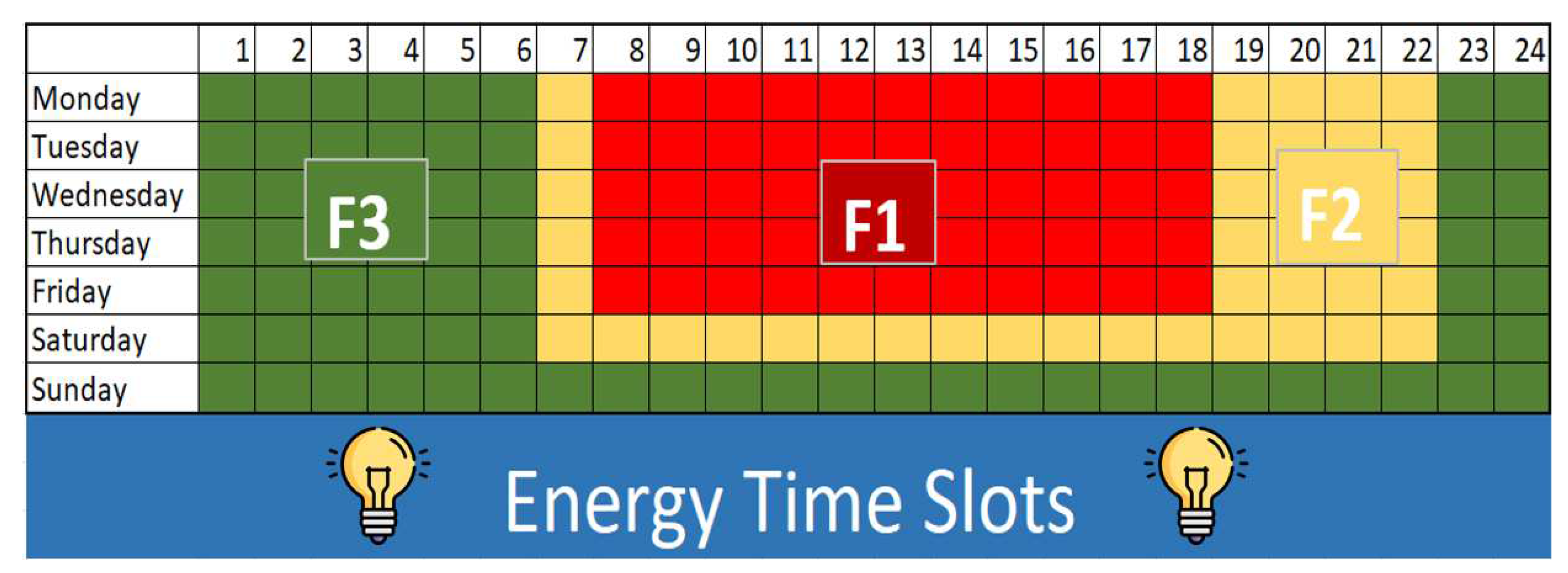
$B_{t}^{el}$ : Price of electricity bought [€/kWh] the price of the electricity to be bought has dynamic pricing depending upon the time slots set by the distribution company based on the F1, F2, and F3 slots as shown below in Figure A1:
$r_{t}^{el}$ : Revenue for electricity sold [€/kWh]
$q_{t}^{el}$ : Price of Reactive power bought [€/kVAR]
$s_{t}^{el}$ : Revenue for Reactive power sold [€/kVAR]
$C^{curt, RES}$ : Cost of curtailment for RES [€/kWh]

To assess the costs specified in the objective function of the optimization model, certain input data must be supplied. Curtailment costs for the RESs have been considered equal to the LCOE for the respective technology and the price of the fuel is at par with the market price:

$C^{curt_PV} = 0.128 [€ / kWh]$ , $C^{curt_W} = 0.6 [€ / kWh]$ , $C^{fuel_CHP} = 0.1137 [€ / kWh]$

Figure A1. Reference for the dynamic pricing for active power bought where F1=0.35[€/kWh], F2=0.25[€/kWh], F3=0.15[€/kWh].

Transformer

$A^{T}$ : Nominal apparent power of the transformer [kVA]
$V^{N 1}$ : Nominal voltage (line to line) primary side [kV]
$V^{N 2}$ : Nominal voltage (line to line) secondary side [kV]
$P^{CC}$ : On Load loss of the transformer [W]
$v^{SC}$ : Short circuit voltage of the transformer [-]

The parameters for the transformer system are as follows: $A^{T} = 800 kVA$ , $V^{N 1} = 15 kV$ , $V^{N 2} = 0.4 kV$ , $P^{C C} = 8000 W$ , and $v^{S C} = 0.06$ .

Storage Batteries

$η^{ch, ESS}$ , $η^{dch, ESS}$ : Charging and discharging efficiencies
$P_{b}^{\max, ch, ESS}$ , $P_{b}^{\max, dch, ESS}$ : Max charging and discharging power [kW]
$P_{b}^{\min, ch, ESS}$ , $P_{b}^{\min, dch, ESS}$ : Min charging and discharging power [kW]
$A_{b}^{ESS}$ : Nominal apparent power of the electrical storage inverter [kVA]
$C_{b}^{ESS}$ : Rated capacity of the storage system [kWh]
$N^{ESS}$ : Number of batteries
${SOC}^{\min, ESS}$ , ${SOC}^{\max, ESS}$ : Min and max state of charge [
$τ^{ESS}$ : Ideal self-discharging rate
$Δ$ : Time interval, where $Δ$ =0.25

Electrical Vehicle (EV)

$P_{b, j, v}^{\max, ch, AC}$ , $P_{b, e, v}^{\max, ch, DC}$ , $P_{b, f, v}^{\max, ch, V 2 G}$ : Max charging powers [kW]
$P_{b, f, v}^{\max, dch, V 2 G}$ : Max discharging power V2G [kW]
$y_{v, t}^{EV}$ : EV availability
${SOC}_{v}^{\min, EV}$ , ${SOC}_{v}^{\max, EV}$ : Min and max state of charge [%]
${SOC}_{v}^{ini}$ : Initial state of charge
${SOC}_{v}^{*}$ , ${SOC}_{v}^{* *}$ : State of charge at arrival and departure [%]
$C_{v}^{EV}$ : Capacity of EV battery [kWh]
$η^{ch, AC}$ , $η^{ch, DC}$ : Charging efficiencies for AC and DC chargers
$η^{ch, V 2 G}$ , $η^{dch, V 2 G}$ : Charging and discharging efficiencies for V2G chargers
$F_{v}^{EV}$ : Vehicle Consumption [kWh/km]
$D_{v, t}^{EV}$ : Vehicle demand [km]
$τ^{dis}$ : Factor for calculating self-discharging

Heat Pump

$γ_{b}^{HP}$ , $σ_{b}^{HP}$ , $ψ_{b}^{HP}$ : Constants from product data sheets
$T_{b, t}^{amb}$ : Ambient temperature
$π_{b}^{HP}$ : Constant from product data sheets
${COP}_{b, t}^{HP} = γ_{b}^{HP} \cdot T_{b, t}^{amb} + σ_{b}^{HP}$ : COP of Heat pump
${EER}_{b, t}^{HP} = ψ_{b}^{HP} \cdot T_{b, t}^{amb} + π_{b}^{HP}$ : EER of Heat pump
$P_{b, t}^{th, HP, \max} (T_{b, t}^{amb})$ : Max thermal power by Heat pump (temperature dependent)
$P_{b, t}^{cool, HP, \max} (T_{b, t}^{amb})$ : Max cooling power by Heat pump (temperature dependent)

The values of the required variables for the heat pump that are required for the optimization are as follows:

$γ_{b}^{HP} = 0.07$ , $σ_{b}^{HP} = 2.6$ , $ψ_{b}^{HP} = - 0.1$ , and $π_{b}^{HP} = 5$ .

Chiller

$P_{b}^{th, chiller, \min}$ : Min thermal output of chiller
$P_{b}^{th, chiller, \max} (T_{b, t}^{amb})$ : Max output of chiller (temperature dependent)
$ρ_{b}^{chiller}$ : Factor for converting cooling energy to electrical energy
Additional data: $ε_{b}^{heating}$ , $ε_{b}^{cool}$ , $ε_{b}^{chiller}$ , $L_{b, t}^{th}$ , $L_{b, t}^{cool}$

The values of the required variables for the chiller that are required for the optimization are as follows:

$ρ_{b}^{chiller} = 0.10$ . The efficiencies for heating, cooling, and the chiller are $ϵ_{b}^{heating} = 0.92$ , $ϵ_{b}^{cool} = 0.92$ , and $ϵ_{b}^{chiller} = 0.95$ respectively.

References

GSR2022-full report, “RENEWABLES 2022 GLOBAL STATUS REPORT,” January 20, 2022, https://www.ren21.net/wp-content/uploads/2019/05/GSR2022_Full_Report.pdf.
Net Zero Tracker, “Post-COP26 Snapshot”, Available online: https://zerotracker.net/analysis/post-cop26-snapshot, accessed January 19, 2022.
Ibid.; T. Gillespie, J. Starn and I. Almeida, “Europe’s Power Crunch Shuts Down Factories as Prices Hit Record,” Bloomberg, December 22, 2021, https://www.bloomberg.com/news/articles/2021-12-22/european-power-surges-to-record-as-francefaces-winter-crunch; US Energy Information Administration (EIA),“Wholesale Electricity Prices Trended Higher in 2021 Due to Increasing Natural Gas Prices,” Today in Energy, January 7, 2022, https://www.eia.gov/todayinenergy/detail.php?id=50798.
Carbon Brief, “COP26: Key Outcomes Agreed at the UN Climate Talks in Glasgow”, November 15, 2021, https://www.carbonbrief.org/cop26-key-outcomes-agreed-at-the-un-climate-talks-in-glasgow.
COP26, “COP26 Presidency Outcomes: The Climate Pact,” November 2021, https://ukcop26.org/wp-content/uploads/2021/11/COP26-Presidency-Outcomes-The-Climate-Pact.pdf.
F. Harvey, J. Ambrose and P. Greenfield, “More than 40 Countries Agree to Phase out Coal-Fired Power,” The Guardian, November 3, 2021, https://www.theguardian.com/environment/2021/nov/03/more-than-40-countries-agree-to-phase-out-coalfired-power; Global Energy Monitor, “Global Ownership of Coal Plants,” Global Coal Plant Tracker, https://globalenergymonitor.org/projects/global-coal-plant-tracker/summary-tables, accessed February 18, 2022.
IEA, op. cit. note 41; IRENA, World Energy Transitions Outlook 2021, 2021, https://irena.org/publications/2021/Jun/World-Energy-Transitions-Outlook.
https://re.jrc.ec.europaeu/pvg_tools/en/.
A. Sawhney, S. Bracco, F. Delfino and B. Bonvini, "Optimal planning and operation of a small size Microgrid within a Positive Energy District," 2022 AEIT International Annual Conference (AEIT), Rome, Italy, 2022, pp. 1-6. [CrossRef]
Zia MF, Elbouchikhi E, Benbouzid M. Microgrids energy management systems: A critical review on methods, solutions, and prospects. Appl Energy 2018;222:1033–55. [CrossRef]
Chen C, Duan S, Cai T, Liu B, Hu G. Smart energy management system for optimal microgrid economic operation. IET Renew Power Gener 2011;5(3):258–67.
F. Katiraei, R. Iravani, N. Hatziargyriou, and A. Dimeas, “Microgrids management,” IEEE Power Energy Mag., vol. 6, no. 3, pp. 54–65, May 2008. [CrossRef]
L. N. An and N.T. Lam T. Q. Tuan, "Optimal energy management strategies of microgrids", IEEE Computational Intelligence (SSCI), 6-9 Dec. 2016. [CrossRef]
N. Zaree and V. Vahidinasab, "An MILP formulation for centralized energy management strategy of microgrids," 2016 Smart Grids Conference (SGC), Kerman, Iran, 2016, pp. 1-8. [CrossRef]
E. Derkenbaeva, S. Halleck Vega, G.J. Hofstede and E. van Leeuwen, "Positive energy districts: Mainstreaming energy transition in urban areas", Renewable and Sustainable Energy Reviews, vol. 153, pp. 111782, 2022. [CrossRef]
IEA EBC Annex 83. Positive energy districts, 2020. [CrossRef]
S. Bossi, C. Gollner and S. Theierling, "Towards 100 positive energy districts in europe: Preliminary data analysis of 61 european cases", Energies, vol. 13, no. 22, 2020. [CrossRef]
O. Lindholm, H. u. Rehman and F. Reda, "Positioning positive energy districts in european cities", Buildings, vol. 11, no. 1, 2021. [CrossRef]
"Urban Europe", Available online:: https://jpi-urbaneurope.eu/.
"Urban Europe – Europe towards positive energy districts: A compilation of projects towards sustainable urbanization and the energy transition – First Update", February 2020.
Alpine Space EU, Available online: https://www.alpine-space.eu/projects/alpgrids/en/home.
"Savona Campus", Available online: https://campus-savona.unige.it/en/.
"Energia 2020 project", Available online: http://www.energia2020.unige.it/en/home/.
IRE Liguria, Available online: http://www.ireliguria.it/eng.html.
G. Bianco, B. Bonvini, S. Bracco, F. Delfino, P. Laiolo and G. Piazza, "Key Performance Indicators for an Energy Community based on sustainable technologies", Sustainability, vol. 13, no. 16, 2021. [CrossRef]
R. H. Byrne, T. A. Nguyen, D. A. Copp, B. R. Chalamala and I. Gyuk, "Energy Management and Optimization Methods for Grid Energy Storage Systems," in IEEE Access, vol. 6, pp. 13231-13260, 2018. [CrossRef]
European Alternative Fuels Observatory, Available online: https://alternative-fuels-observatory.ec.europa.

Figure 1. Exsisting Savona campus and Pilot project site.

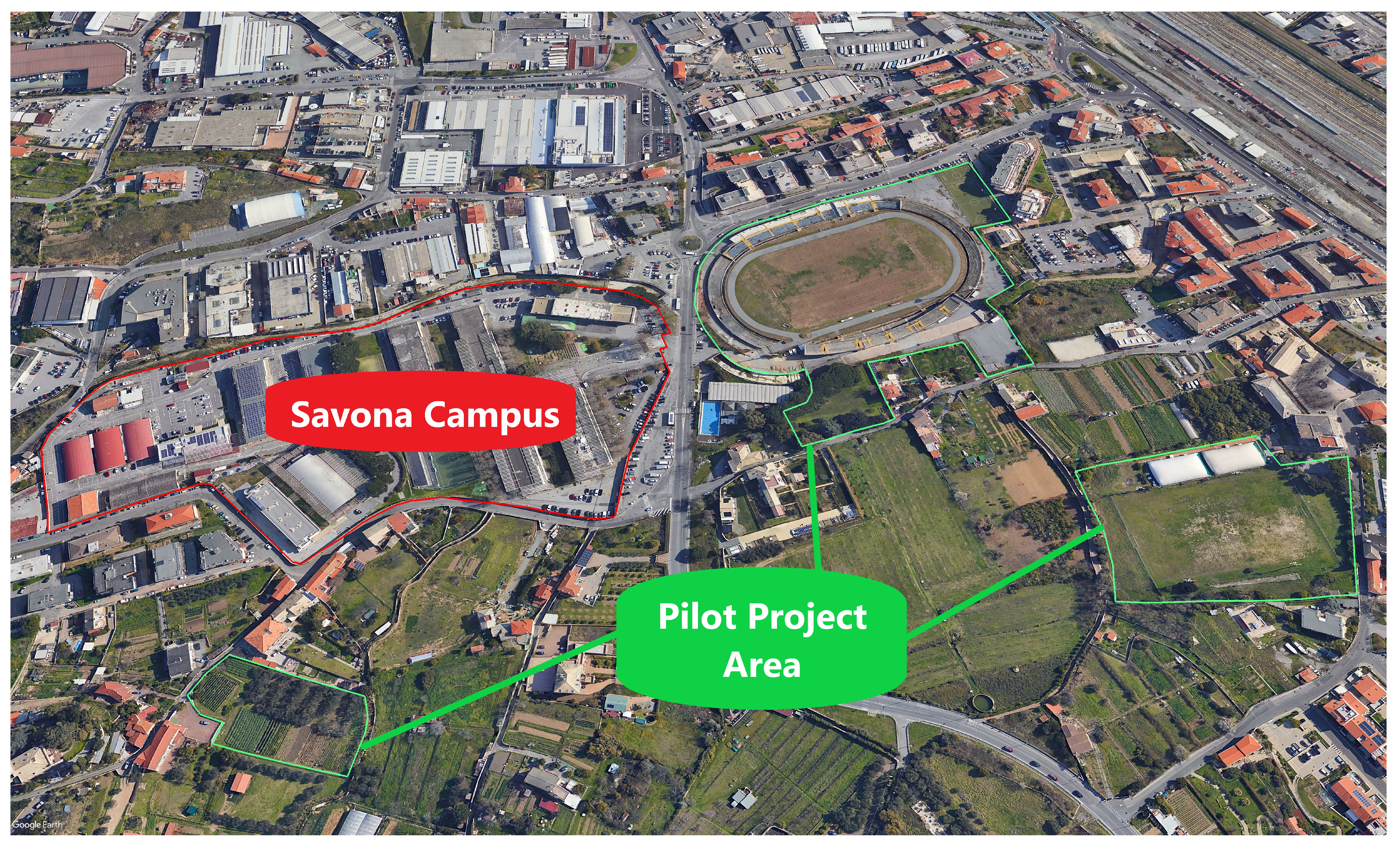
Figure 2. The microgrid’s architecture with its components.

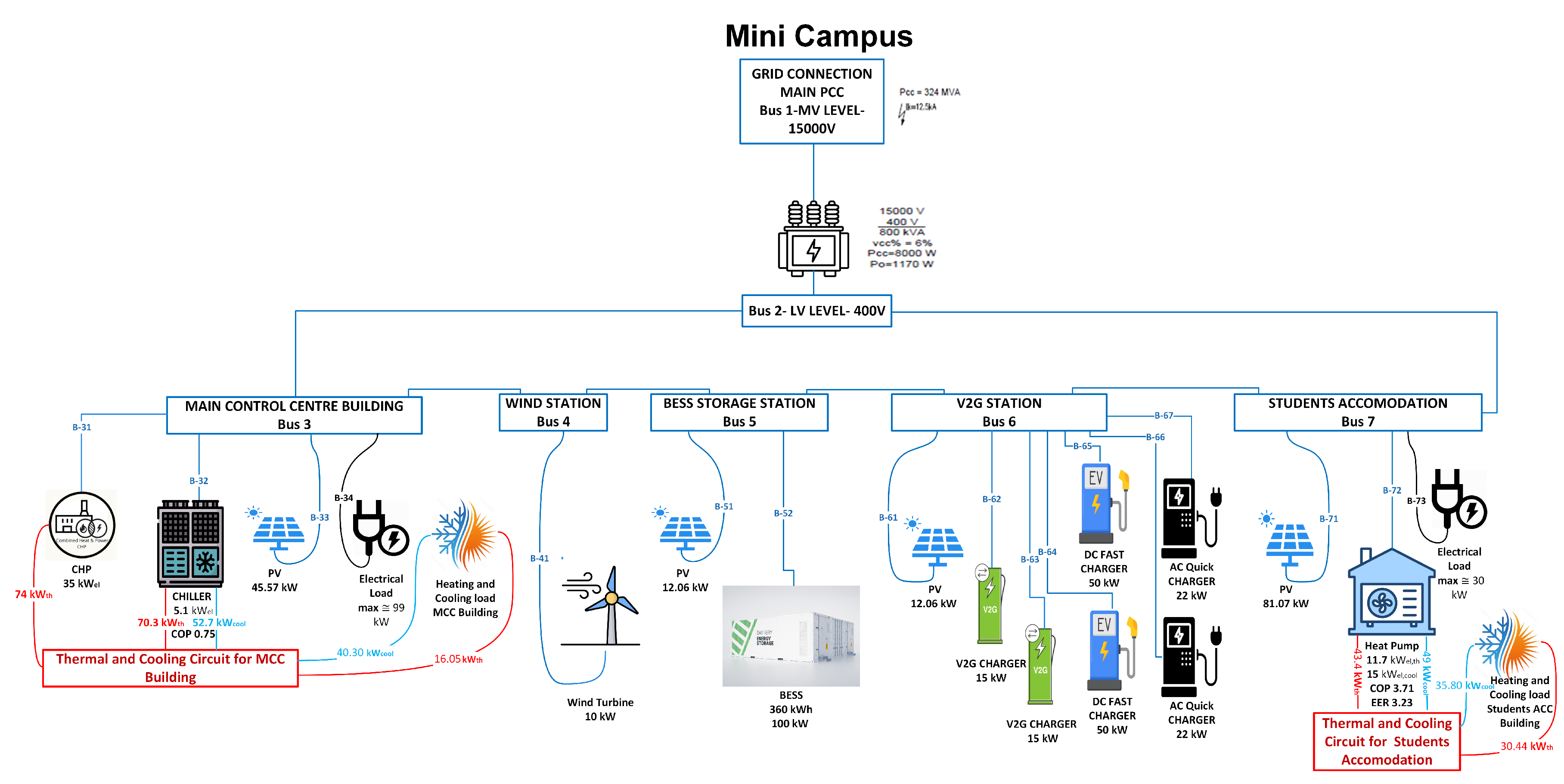
Figure 3. Cars Demand profile graphs.

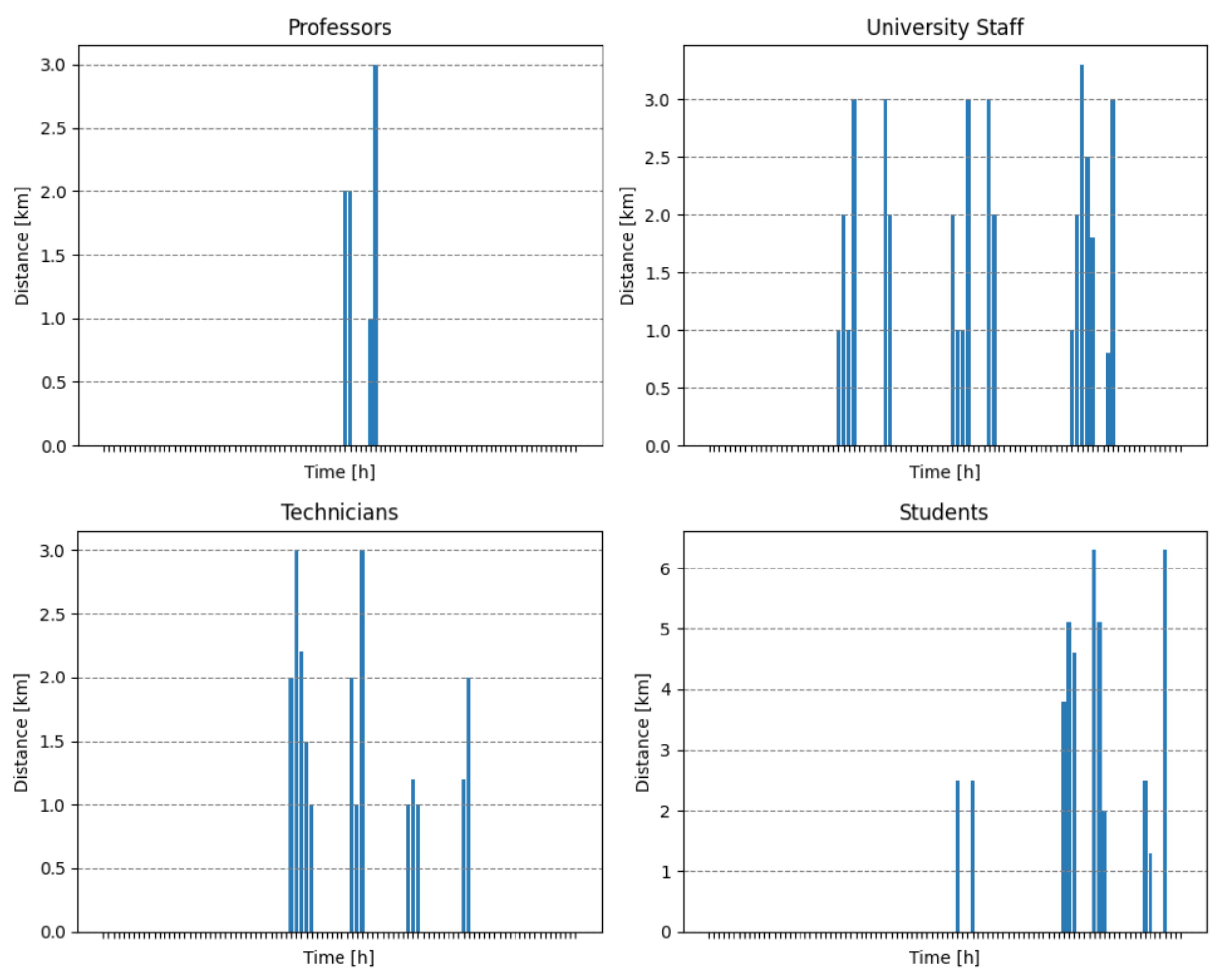
Figure 4. Active and Reactive power flow on a typical summer day.

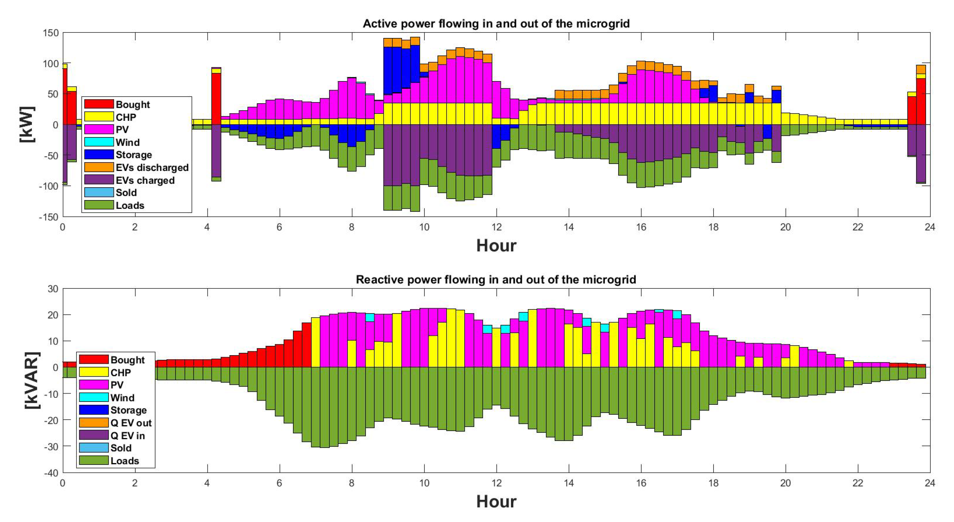
Figure 5. Voltage profiles of all the 7 buses.

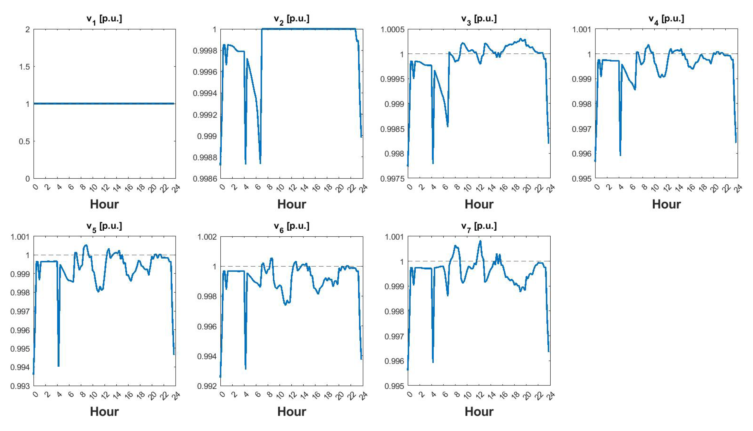
Figure 6. PV inverter capability curve. Pink stars represent the hourly operating points of the inverter. The yellow semi-circular line represents the non-linearized capability curve of the inverter. The blue dashed line represents the rectangular capability curve chosen for the PV technology.

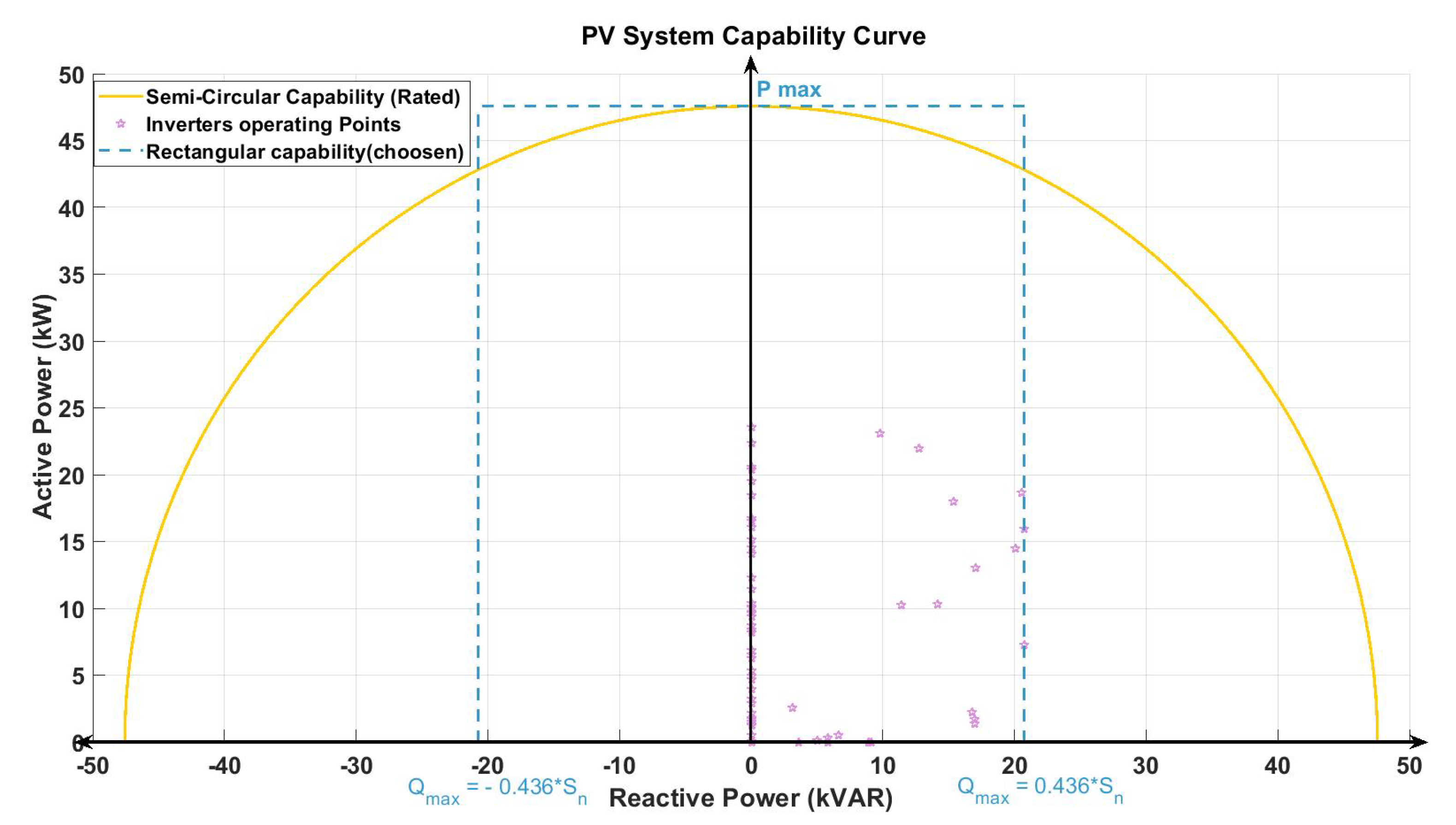
Figure 7. Active and Reactive power flow across different buses in [kW] and [kVAR] respectively.

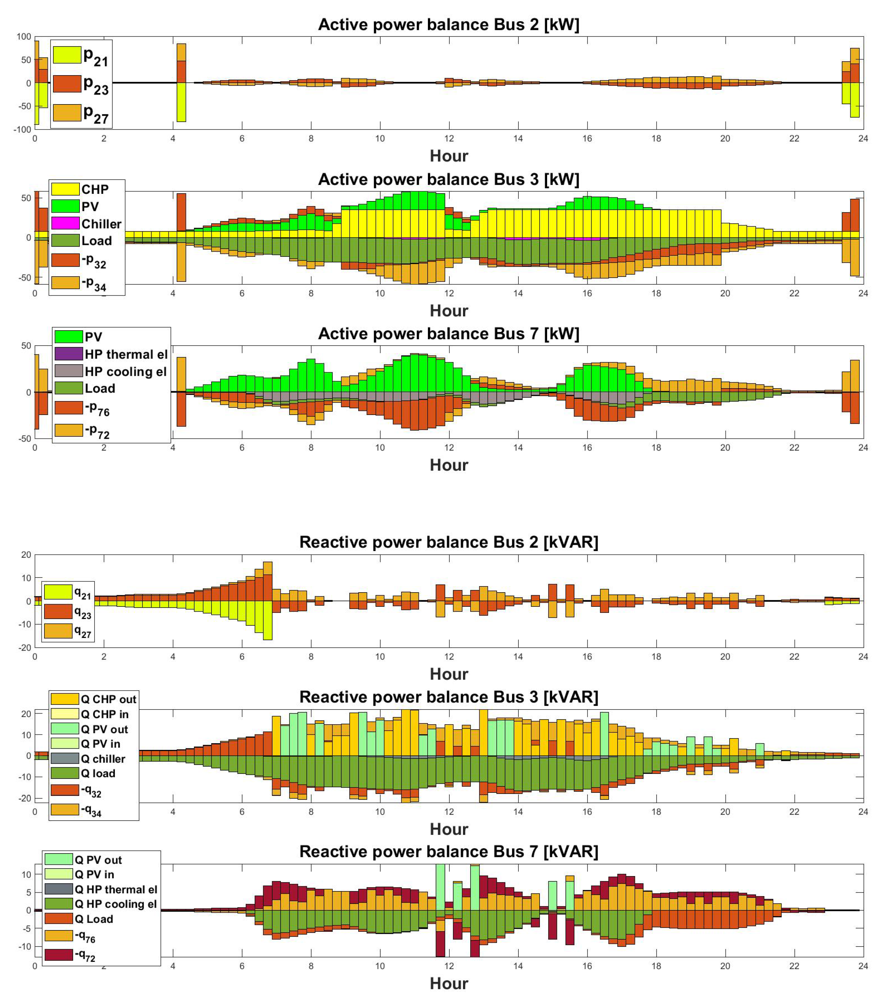
Figure 8. EV 1 and 9 Demand, SOC and EV’s charging and discharging power.

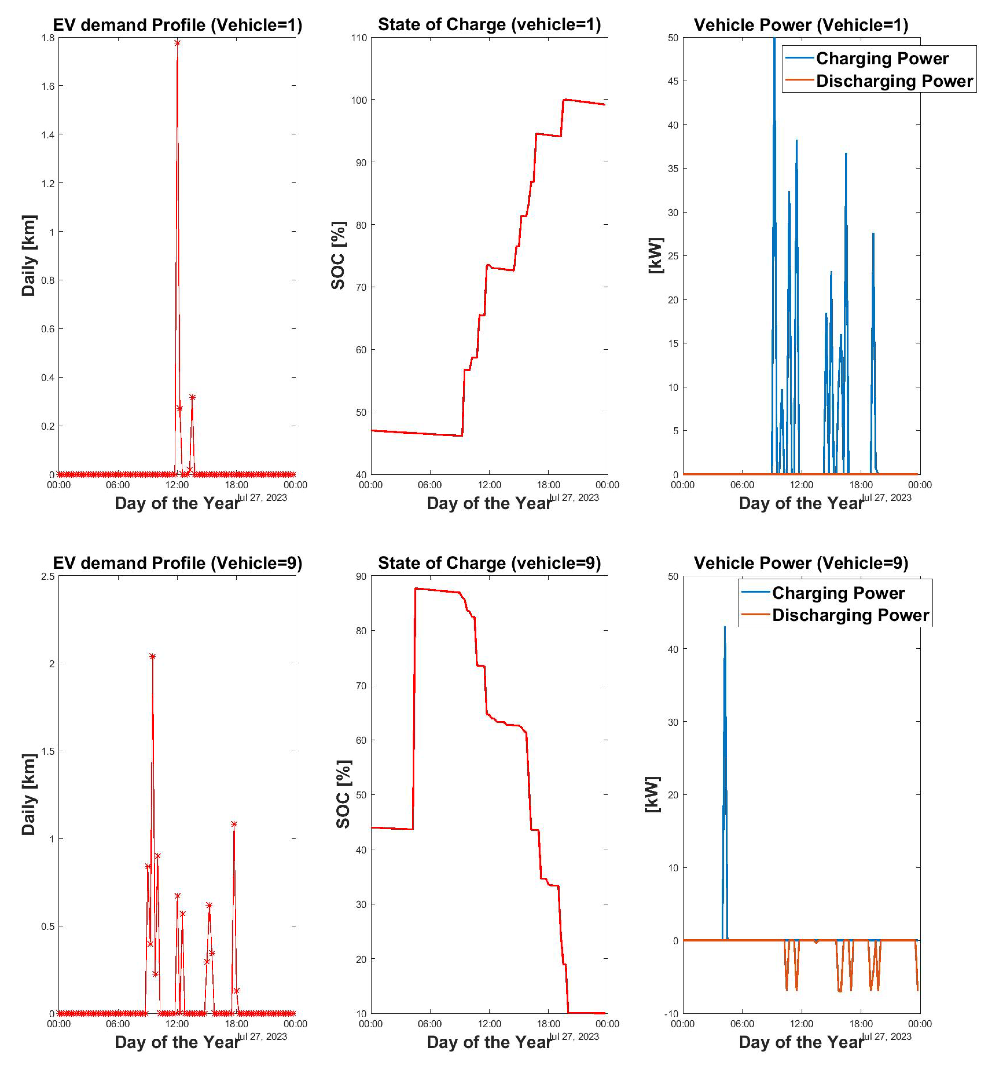
Figure 9. Active and reactive power flow in the bus 2, bus 3, bus 7.

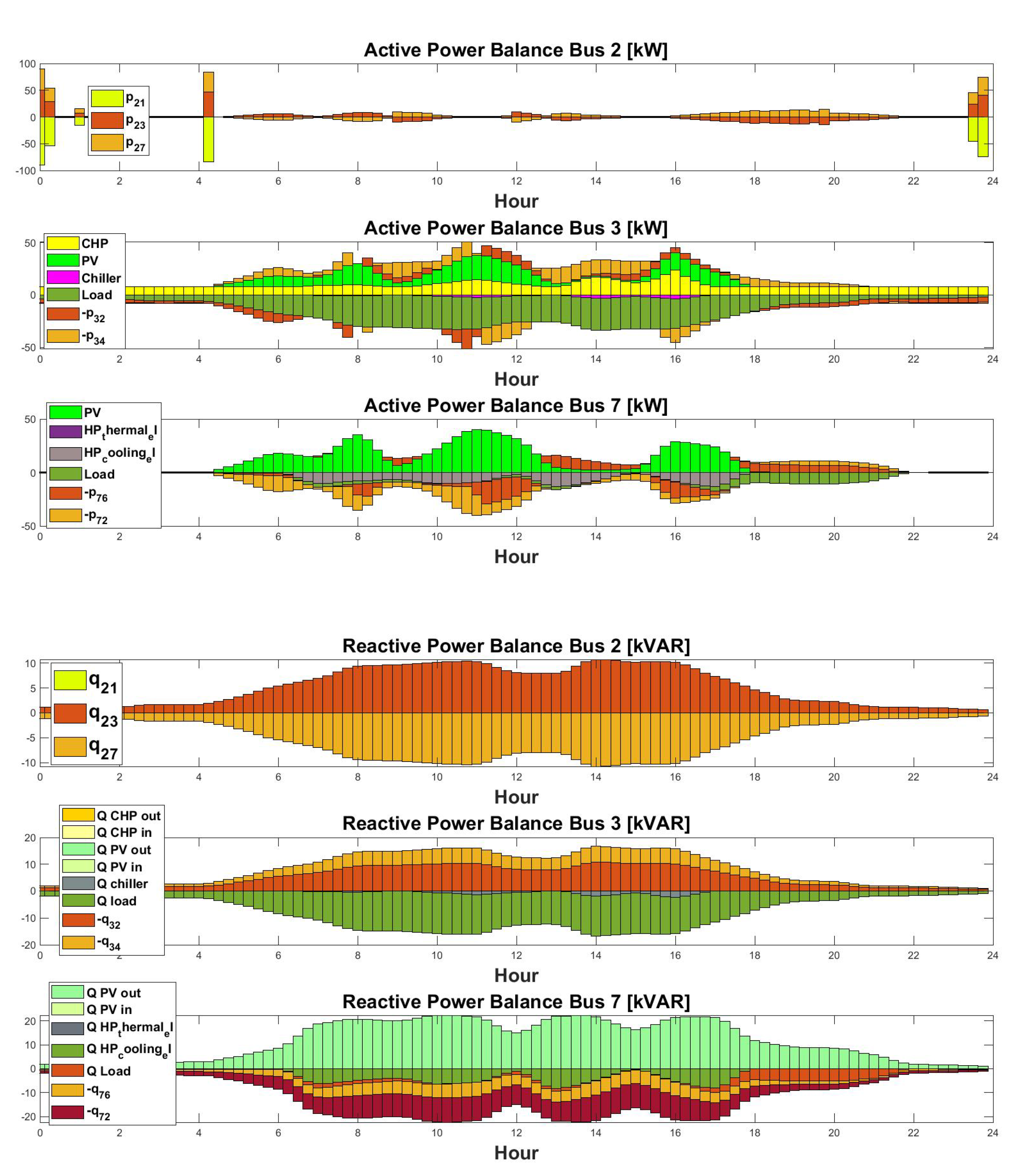
Figure 10. Active and reactive power balance of microgrid on typical winter day with E-mobility.

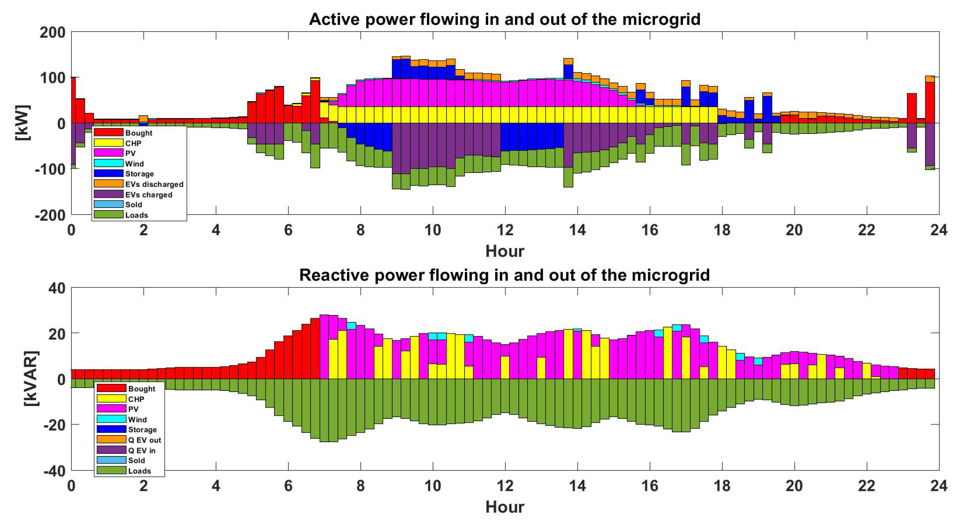
Figure 11. Voltage profile of different buses on typical winter day With EV.

Figure 12. Active and Reactive power flow in different buses with EV on typical winter day.

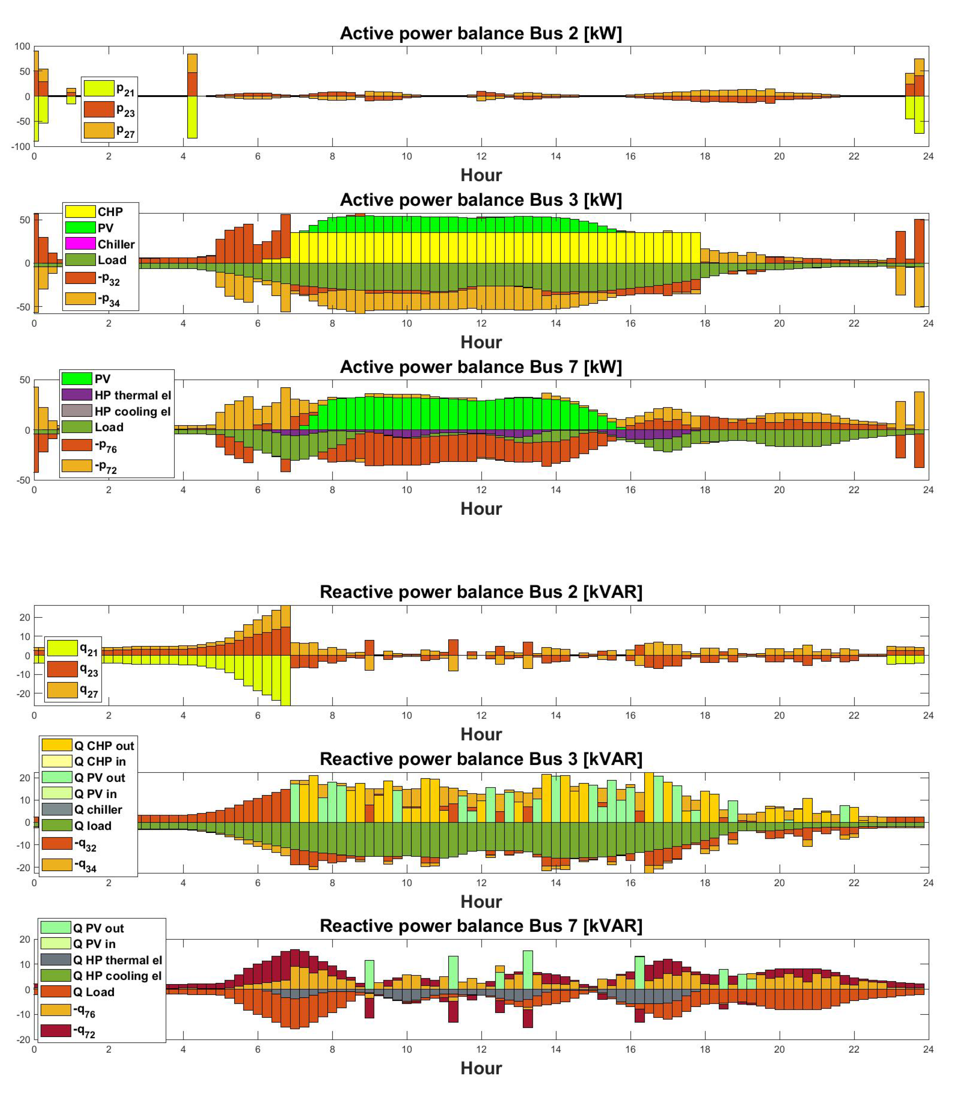
Figure 13. Profile of car 1 and car 8 with demand, SOC and charging and discharging power.

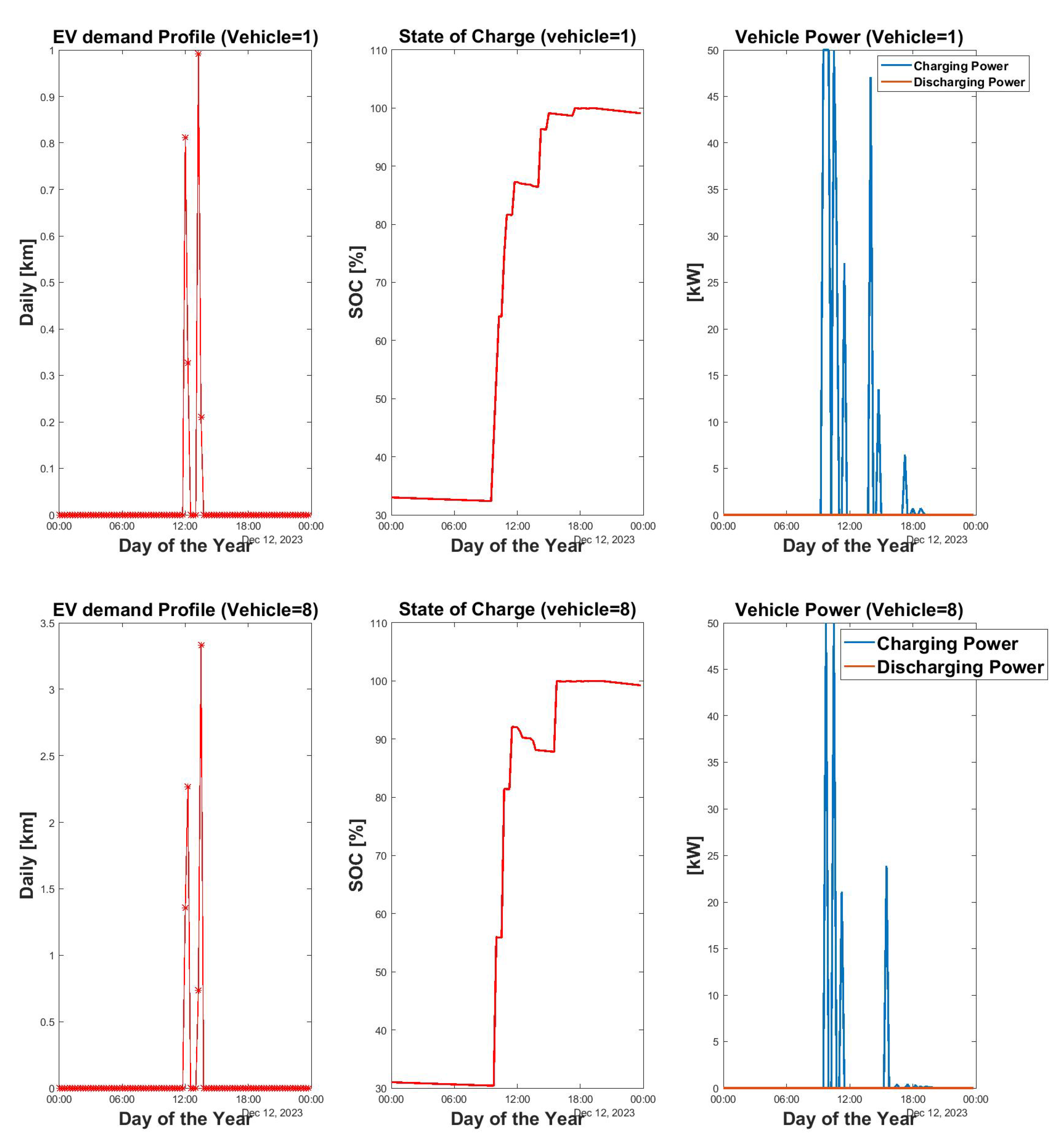
Figure 14. Active and Reactive power flow in different buses without EV on typical winter day.

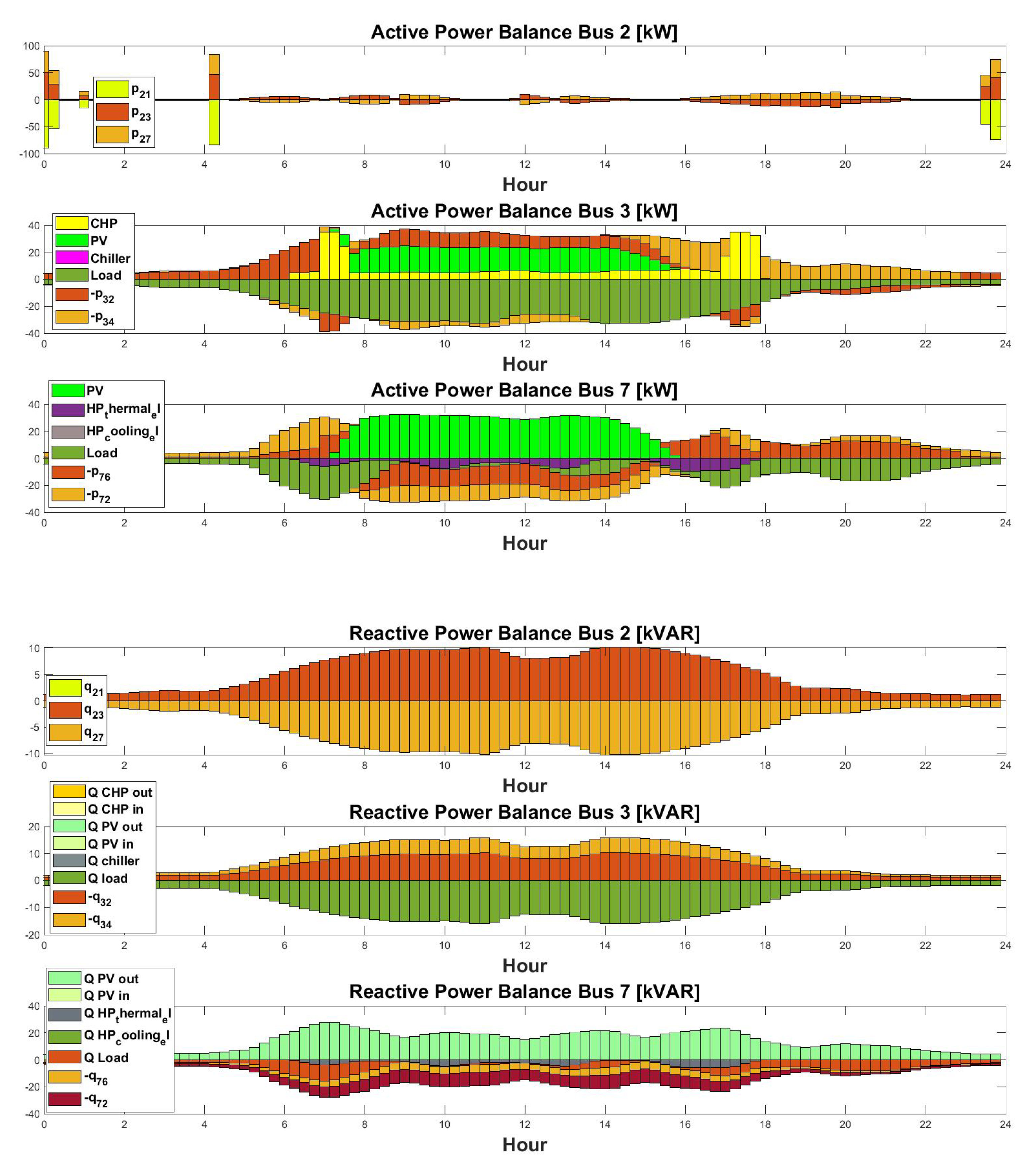
Figure 15. Active and reactive power balance of microgrid on typical offseason day with E-mobility.

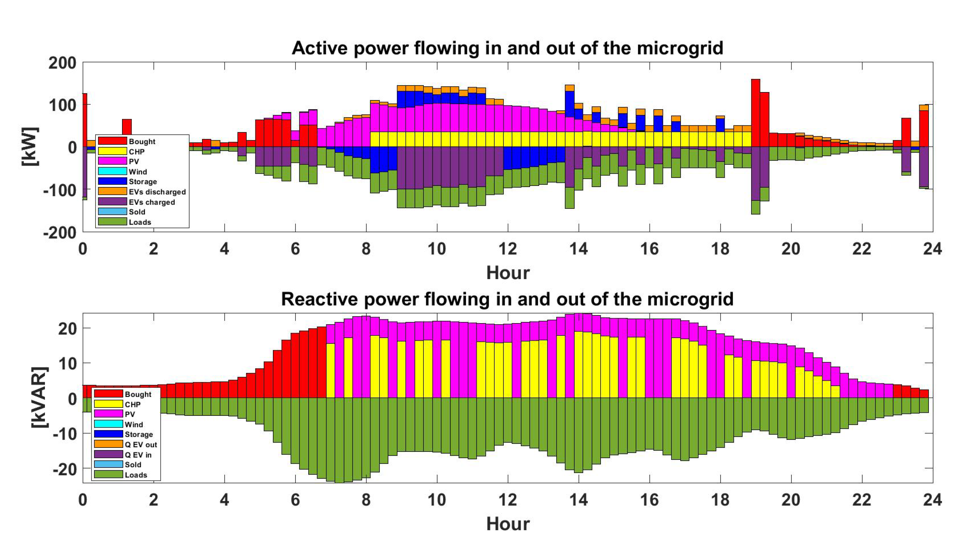
Figure 16. Voltage profile for different buses for a typical off-season day.

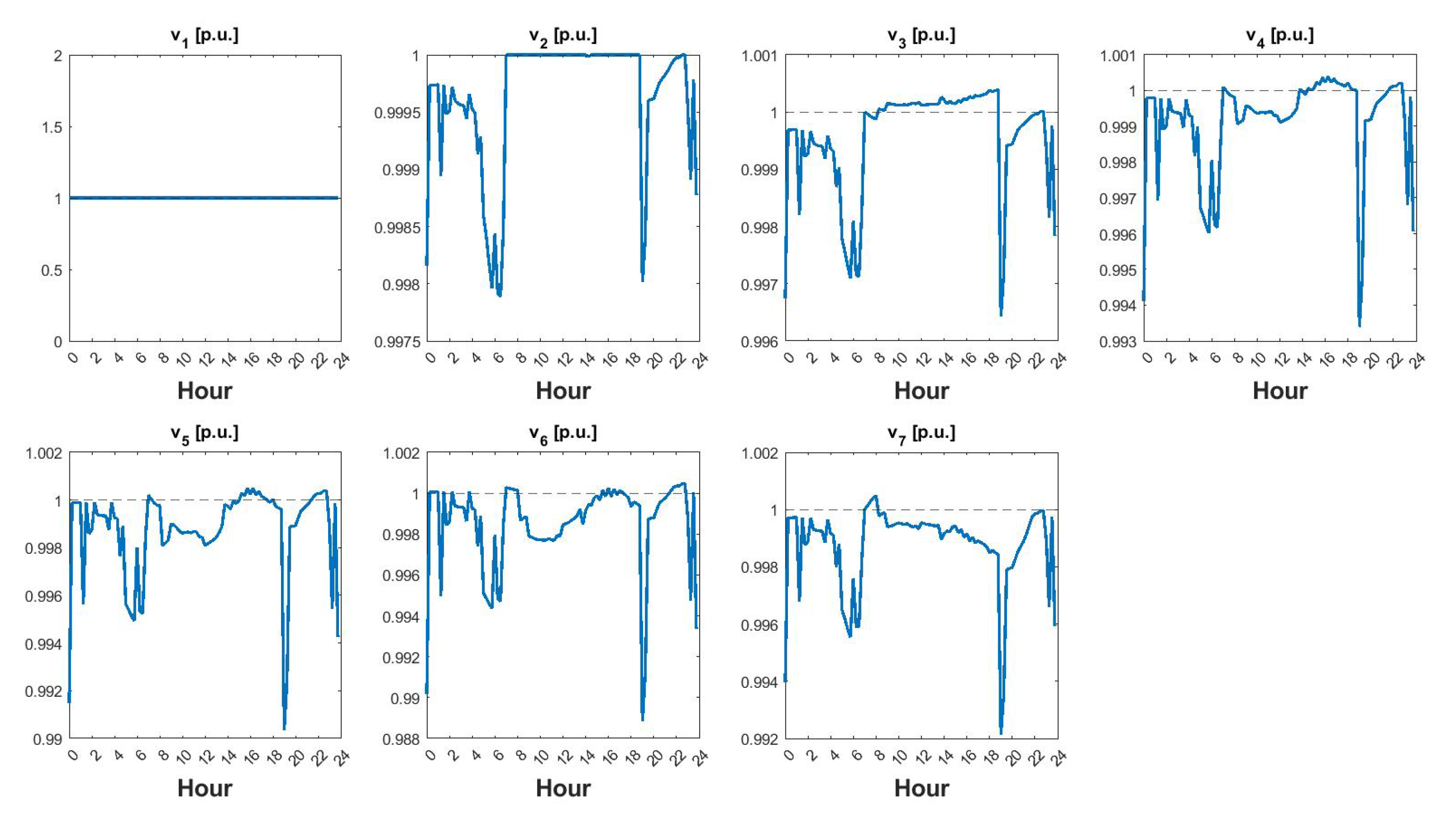
Figure 17. Car 9 and car 13 Demand profile, SOC and charging and discharging power.

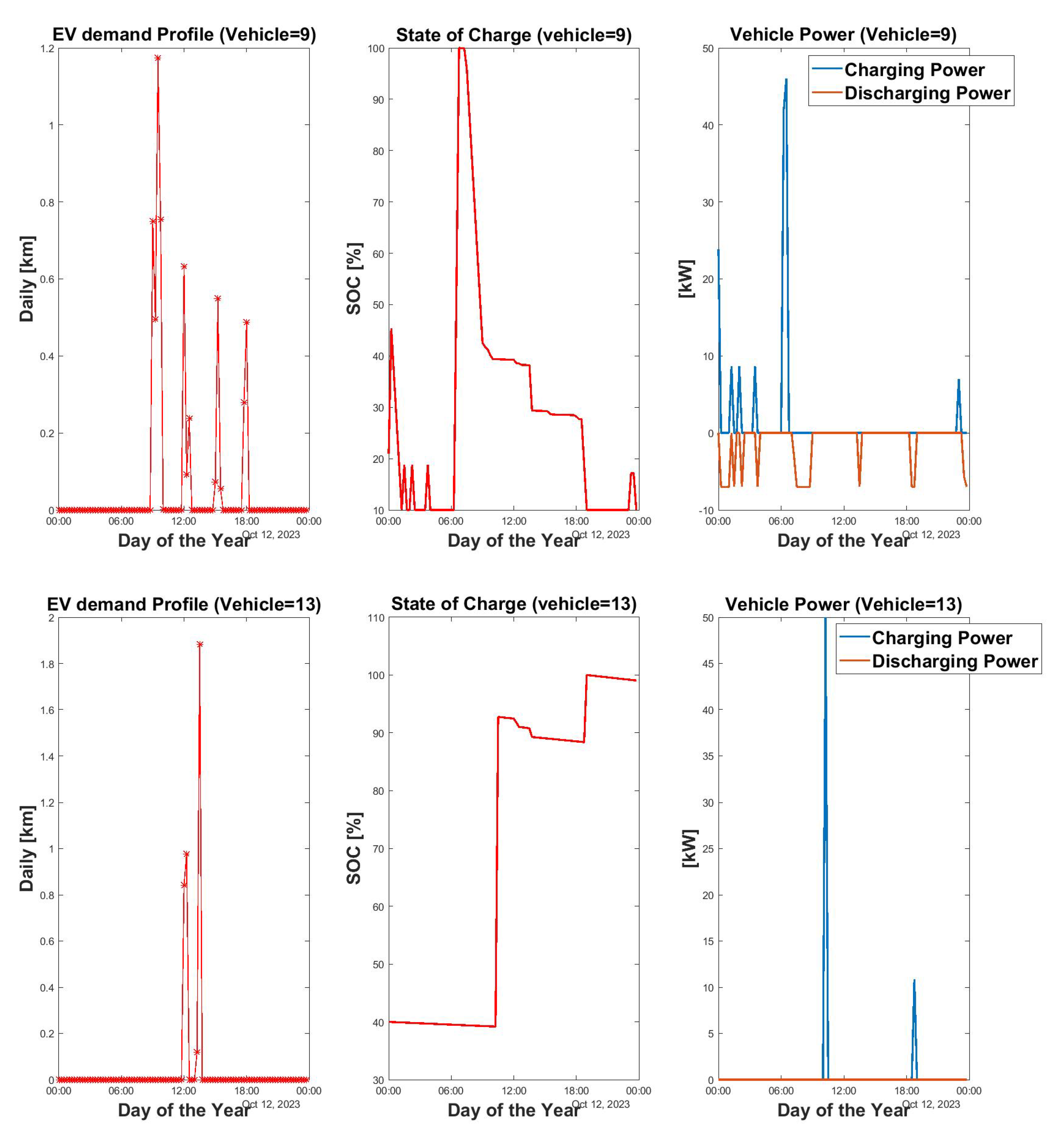
Figure 18. Active and reactive power flow across different profiles on an off-season day.

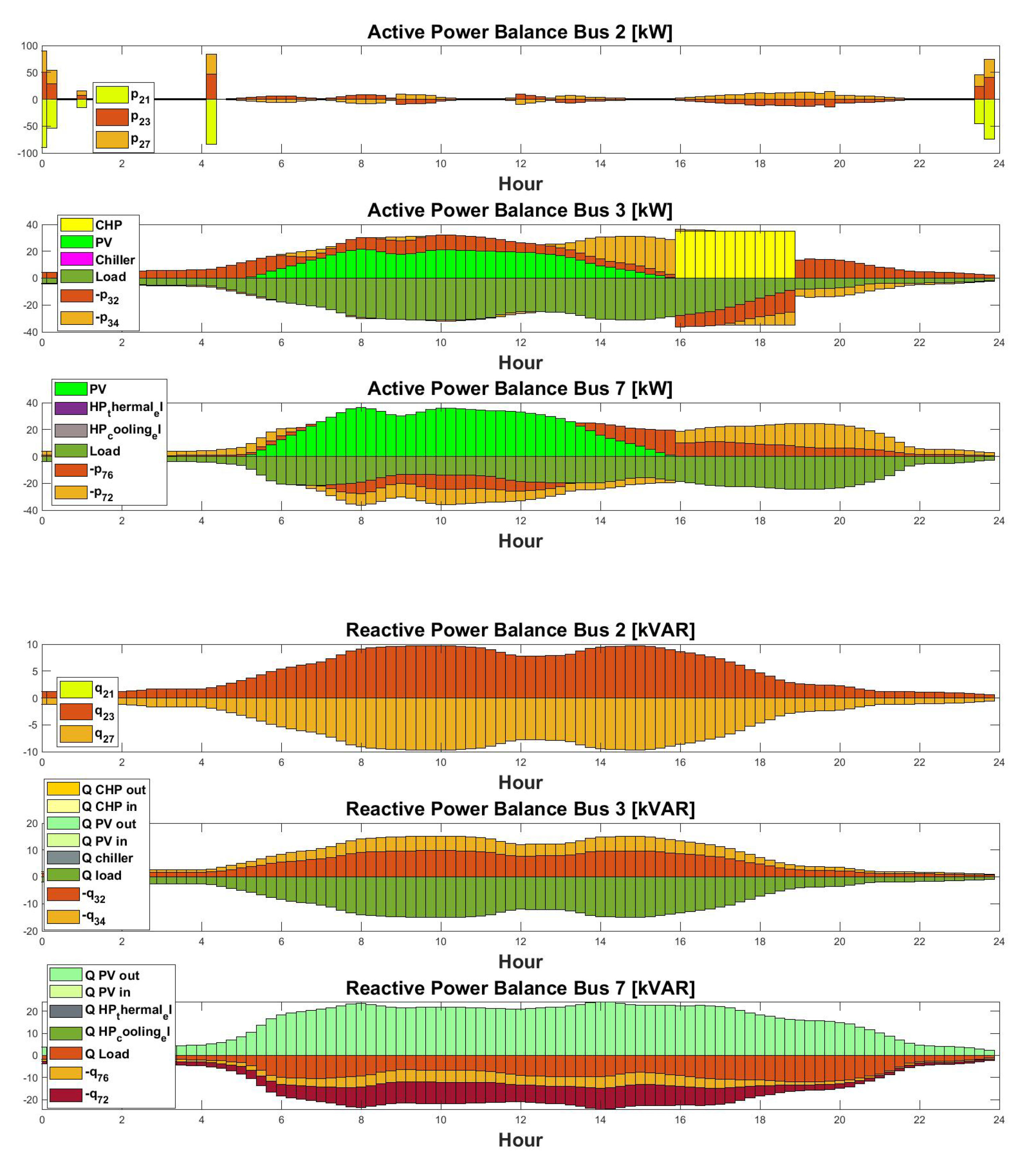
Table 1. Selected Cars and their specifications.

Car Model number	Charging Mode	Battery Type	Total no of Cars	Battery useable capacity [kWh]	Range [km]	Vehicle Consumption [Wh/km]	AC charging [kW]	DC Fast charging [kW]	V2G charging [kW]	V2G discharging [kW]
Audi Q8 e-tron 55 quattro	AC/DC	Lithium-ion	1	106	495	214	22	50	15	0
Nissan Leaf e+	AC/DC/V2G	Lithium-ion	3	59	340	174	7	46	15	7
Tesla Model X Plaid	AC/DC	Lithium-ion	1	95	455	209	11	50	15	0
Renault Kangoo E-Tech Electric	AC/DC	Lithium-ion	2	44	215	205	22	50	15	0
Fiat 500e Cabrio	AC/DC	Lithium-ion	2	21	135	158	11	50	15	0
Renault Zoe ZE50 R135	AC/DC	Lithium-ion	1	52	310	135	22	46	15	0
Nissan e-NV200 Evalia	AC/DC/V2G	Lithium-ion	1	22	105	210	7	46	15	7
Smart EQ fortwo coupe	AC	Lithium-ion	3	17	100	167	22	0	0	0

Table 2. Charging Station Data.

Charging Station	No of Chargers	Max Power [kW]
AC	2	22
DC	2	50
V2G⁴	2	15

⁴ Discharging power 7 [kW].

Table 3. Size of different Technologies.

Bus Number	Size of PV plant [kWp]	Size of CHP engine [kWel]	Size of $μ$ Wind turbine [kW]	BESS Size [kWh]
BUS 1	0	0	0	0
BUS 2	0	0	0	0
BUS 3	45.57	35	0	0
BUS 4	0	0	10	0
BUS 5	12.06	0	0	360
BUS 6	12.06	0	0	0
BUS 7	81.07	0	0	0

Table 4. Technology Data

Technology	Thermal Capacity [kWth]	Cooling Capacity [kWcool]
Absorption Chiller	0	52.7
CHP¹	74	0
Heat Pump^2,3	43.4	49

¹ Power consumption 5.1 [kWel]. ² Power consumption 11.7 [kWelcool]. ³ Power consumption 15 [kWelth].

Table 5. Building Data

Building	Electrical Peak Load (kWel)	Thermal Peak Load [kWth]	Cooling peak Load [kWcool]
MCC Building	99	16.05	40.3
Students Accommodation	30	30.44	35.8

Disclaimer/Publisher’s Note: The statements, opinions and data contained in all publications are solely those of the individual author(s) and contributor(s) and not of MDPI and/or the editor(s). MDPI and/or the editor(s) disclaim responsibility for any injury to people or property resulting from any ideas, methods, instructions or products referred to in the content.

© 2023 by the authors. Licensee MDPI, Basel, Switzerland. This article is an open access article distributed under the terms and conditions of the Creative Commons Attribution (CC BY) license (http://creativecommons.org/licenses/by/4.0/).

Copyright: This open access article is published under a Creative Commons CC BY 4.0 license, which permit the free download, distribution, and reuse, provided that the author and preprint are cited in any reuse.

MDPI Initiatives

Important Links

Choose an area of interest and we will send you notifications of new preprints at your preferred frequency.

Disclaimer

EMS for Active and Reactive Power Management in a Polygenerative Microgrid feeding a PED

Abstract

1. Introduction

1.1. Fundamentals, Evolution, and Classification of Energy Management Systems

2. PED and Alpgrids Project

2.1. Positive Energy Districts (PED)

2.2. Alpgrids Project

3. EMS: Application and Mathematical Model

3.1. Structure and Elements of the Microgrid

3.2. Mathematical Model

3.2.1. Distributed Generation Model

3.2.2. BESS Model

3.2.3. Grid Model

3.2.4. EV and Wall Box Model

3.2.5. Heating and Cooling System Modeling

3.2.6. Active & Reactive Power Balance

3.2.7. Load Flow Constraints

3.2.8. Objective Function: Minimization of Operating Costs

4. Input Data: Acquisition and Processing

4.1. Electric Mobility

4.2. Specifications of Charging Stations

4.3. Different Technologies Size Estimation

4.4. Load Profile Estimation

5. Results

5.1. Analysis of Different Cases (Typical Days)

5.1.1. Typical Summer Day

5.1.2. Typical Winter Day

5.1.3. Off-Season Day

6. Conclusions

Author Contributions

Funding

Data Availability Statement

Conflicts of Interest

Abbreviations

Appendix A

Appendix A.1. Mathematical Formulas and Definitions

References

MDPI Initiatives

Important Links

Subscribe