

Submitted:
28 December 2023
Posted:
28 December 2023
You are already at the latest version
Abstract
We prove through path integral Monte Carlo computer experiments that the affine quantization of the \(\varphi_4^4\) scaled Euclidean covariant relativistic scalar field theory is a valid quantum field theory with a well defined continuum limit of the one- and two-point-function. Affine quantization leads to a completely satisfactory quantization of field theories using situations that involve scaled behavior leading to an unexpected, \(\hbar^2/\varphi^2\) which arises only in the quantum aspects.
Keywords:
Field theory
; affine quantization
; continuum limit
; Green function
1. Introduction
It is well known that quantum Euclidean covariant relativistic field theory when quantized through canonical (Dirac [1]) quantization (CQ) is non-renormalizable since its corresponding renormalized theory tends to a free theory in the continuum limit [2,3,4,5,6].
Recently J. R. Klauder [7,8,9,10,11] noticed that this difficulty can be overcome by using a different kind of quantization method, namely affine quantization (AQ).
In a sequel of recent papers [12,13,14,15,16,17,18,19,20,21,22] we proved, through path integral Monte Carlo (PIMC), that indeed affine quantization is able to make the theory non-trivial. A crucial point left unanswered in these papers was the validity of the continuum limit at the level of the one- and two-point-functions.
The aim of the present work is to show that as we approach the continuum on the computer, the one- and two-point-function converge to well defined results. In other words we prove the validity of the continuum limit for the field theory quantized through affine quantization.
2. Field theory formulation
For a scalar field, , with spacial degrees of freedom and canonical momentum , the classical affine variables are and . The reason we insist that is because if then whatever is .
We then introduce the classical Hamiltonian expressed in affine variables. This leads us to
where r is a positive, even, integer and is the bare coupling constant such that for we fall into the free field theory. With these variables we do not let otherwise which is not fair to and, as we already observed, we must forbid also which would admit giving again an undetermined kinetic term. Therefore the AQ bounds forbid any nonrenormalizability [12,13,14,15,16,17,18,19,20,21,22] which is otherwise possible for CQ [2,3,4,5].
The quantum affine operators are the scalar field and the dilation operator where the momentum operator is . Accordingly for the self adjoint kinetic term (note that the factor that holds for should be replaced by a factor 2 if [17]) and one finds for the quantum Hamiltonian operator
The affine action is found adding time, , where c is the speed of light constant and t is the Euclidean imaginary time, so that , with H the semi-classical Hamiltonian corresponding to the one of Eq. (2), will then read
where with an abuse of notation we here use x for and , with the Boltzmann’s constant and T the absolute temperature. In this work we will set .
The vacuum expectation value of an observable will then be given by the following expression
where the functional integrals will be calculated on a lattice using the PIMC method as explained later on.
The theory considers a real scalar field taking the value on each site x of a periodic n-dimensional lattice, with space-time dimensions, of lattice spacing a, the ultraviolet cutoff, spacial periodicity and temporal periodicity . The field path is a closed loop on an n-dimensional closed surface of an -dimensional -periodic cylinder of radius L: an -dimensional torus. We used a lattice formulation of the AQ field theory of Eq. (3) (also studied in Eq. (8) of [12]) using additionally the scaling and which is necessary to eliminate the Dirac delta factor divergent in the continuum limit . The affine action for the field (in the primitive approximation [23]) is then approximated by
where is a vector of length a in the direction with . We will have .
In this work we are interested in reaching the continuum limit by taking fixed and letting at fixed volume .
We performed a PIMC [23,24,25,26] calculation for the AQ field theory described by the action of Eq. (5) in natural Planck units . Specifically we studied the and case. We calculated the renormalized coupling constant and mass defined in Eqs. (11) and (13) of [12] respectively, measuring them in the PIMC through vacuum expectation values like in Eq. (4). In particular and , where is the Fourier transform of the field and we choose the 4-momentum with one spacial component equal to and all other components equal to zero. We also calulated the one-, two-point-, and two-point-connected-function, respectively given by
By construction, these are periodic functions, , of period L. Moreover, since the action contains only even powers of the field these functions must be symmetric respect to , namely .
3. The scaling
As we have seen we decided to work with a scaled field , related to the variable , used for example in [12], by
In other words, we are renormalizing the bare field. This can be compared with the standard renormalization formula
is referred to as the renormalized field and Z is called the renormalization constant. In this language, we are setting .
At the same time, we are rescaling the coupling constant with
In the Standard Model, the various coupling constants also need to be renormalized for the continuum limit to exist, but the renormalization is not simply given by a power of the lattice spacing. Instead, it needs to carefully be tuned to the cutoff and to the couplings. In perturbation theory of canonical , the bare coupling constant can be expressed in terms of the renormalized one, order by order. The result consists of a series that starts with :
The standard renormalization procedure is based on the fact that the Fourier transform of the renormalized two-point-function contains a pole at , where M is the physical mass of the particle. The renormalization constant Z is chosen such that the residue of this pole is equal to 1. This ensures, in particular, that and as well as and g have the same dimension. Note that our rescaling (9) and (11) instead changes the dimension of these objects.
We will soon see, in our first case study below, that the expectation value tends to a constant when N becomes large. This means that the expectation value of the unscaled field, , tends to infinity in proportion to [12,14].
As we are holding constant, the unscaled coupling constant g tends to zero in proportion to . This suggests that, for the parameter values we consider, the connected Green’s functions of the unscaled model tend to those of a free scalar field.
4. Numerical results
Our PIMC simulations use the Metropolis algorithm [24,25] to calculate the ensemble average of Eq. (4) which is a multidimensional integral. The simulation is started from the initial condition for all lattice points x, with a small positive number. One PIMC step consisted in a random displacement of each one of the field values, , as follows
where is a uniform pseudo random number in and is the amplitude of the displacement. Each one of these moves is accepted if where is the change in the action due to the move (it can be efficiently calculated considering how the kinetic part and the potential part change by the displacement of a single ) and rejected otherwise. The amplitude is chosen in such a way to have acceptance ratios as close as possible to and is kept constant during the evolution of the simulation. One simulation consisted of M PIMC steps. The statistical error on the average will then depend on the correlation time necessary to decorrelate the property , , and will be determined as , where is the intrinsic variance for .
We used up to a lattice of points () and up to corresponding to PIMC displacement moves.
4.1. First case study
In our simulation we first chose the following study case and .
Notice that the minima of the two symmetric potential wells in the semi-classical Hamiltonian density described by the function , are at . From our Monte Carlo simulations (see Teble 1), it seems that the vacuum expectation value of the field (one-point-value), , tends to these values in the continuum limit, . Note that in some of our previous works [16,18,19] where, instead of keeping the bare mass m constant, we tuned it so to have a constant renormalized mass we found in all cases. This is due to the fact that as N increases so does the necessary bare mass which keeps constant . So that the two symmetric potential wells in the semi-classical Hamiltonian density has minima that tends to zero and one experiences tunneling of the potential barrier at .
In Table 2 we show the values for the renormalized mass, , and coupling constant at increasing values of . We see that in the continuum limit and , meaning that
In Figure 1 we show at increasing values of . From the plot of the simulation data we see that the function is symmetric respect to as expected, since the action only contains even powers of the field.
In Figure 2 we show at increasing values of . From the plot of the simulation data we see that . The width of the spike of at seems to be related to the value of the renormalized mass .
Alternatively we could have adjusted, at each change of N, the value of the bare mass m so to have a fixed value for the renormalized mass . This would have resulted in a convergence towards a unique two-point-connected-function in the continuum limit . We did not choose did strategy because it is numerically problematic to tune the bare mass so to have at each N the same value for the renormalized mass. This was what we did in some of our previous papers [12,13,16,17,18,19,20,21,22].
4.2. Second case study
For the parameter values we just used, the box plays a crucial role: the bare Compton wavelength () is equal to the size L of the box. In order for the box to be a purely technical device introduced to regularize the theory, it must be large compared to the correlation length of the model. At the same time, the lattice spacing must be small compared to it:
Therefore, next we considered the study case with , and , which should be much less affected by the presence of the box than the previous choice .

Table 2.
Renormalized mass , renormalized coupling constant , and one-point-value (vacuum expectation value of the field) for , , and . In our PIMC simulations we used Eqs. (4) and (5).
| N | V | ||
|---|---|---|---|
| 4 | 0.1461(2) | 2.01199(2) | 0.6672(4) |
| 7 | 0.0627(1) | 2.001154(4) | 0.5992(3) |
| 13 | 0.02463(5) | 1.999844(2) | 0.5169(2) |
| 25 | 0.00867(5) | 2.000069(7) | 0.4359(3) |
Notice that the minima of the two symmetric potential wells in the semi-classical Hamiltonian density described by the function , , are such that
So with our choice of we will find, in the continuum limit, in agreement with the results in Refs. [12,13,16,18,19,20,21,22].
From Figure 3 we see the continuum limit , of the scaled two-point-connected-function where, with an abuse of notation, we dropped from , the prime, adopted rigorously in Section 3. Respect to the work [14] (see Fig. 3 there) which dealt with the unscaled free field case and was found to increase with increasing N we see how now the scaling has the effect of letting the value of decrease with increasing N, as shown in Figure 3, since and . It is only tuning the bare mass m so to have a constant renormalized mass for each N, that we would find true convergence. Unfortunately this procedure is not easily accomplished numerically since for each N we would have to make several test runs with different values of m in order to find the value which keeps approximately constant. This procedure was nonetheless carried out in the following works [12,13,16,18,19,20,21,22].
5. Conclusions
In this paper, we represent by . To insure proper values for it is necessary to restrict as well as . Indeed such symbol change is able to treat Hamiltonian densities with an interaction . This leads to a completely satisfactory quantization of field theories using situations that involve scaled behavior leading to an unexpected, which arises only in the quantum aspects. Indeed, it is fair to claim that this symbol change leads to valid field theory quantizations.
Respect to the work [14] which dealt with the free field case we here repeat that analysis but now for the interacting case.
We prove through path integral Monte Carlo computer experiments that the affine quantization of the scaled Euclidean covariant relativistic field theory is a well defined quantum field theory with a well defined continuum limit of the one- and two-point-function, the Green’s function.
The simple pseudo-potential stemming from the affine quantization procedure [9] not only does not disturb the continuum limit, as we proved here, but in addition is able to render renormalizable the theory which is known [2] to be non-renormalizable when treated with the more commonly known [1] canonical quantization.
References
- Dirac, P.A.M. The Principles of Quantum Mechanics; Claredon Press: Oxford, 1958; in a footnote on page 114. [Google Scholar]
- Freedman, B.; Smolensky, P.; Weingarten, D. Monte Carlo Evaluation of the Continuum Limit of and . Physics Letters 1982, 113B, 481. [Google Scholar] [CrossRef]
- Aizenman, M. Proof of the Triviality of Field Theory and Some Mean-Field Features of Ising Models for d>4. Phys. Rev. Lett. 1981, 47, 886. [Google Scholar] [CrossRef]
- Fröhlich, J. On the Triviality of λ Theories and the Approach to the Critical Point in d≥4 Dimensions. Nuclear Physics B 1982, 200, 281. [Google Scholar] [CrossRef]
- Siefert, J.; Wolff, U. Triviality of φ4 theory in a finite volume scheme adapted to the broken phase. Physics Letters B 2014, 733, 11. [Google Scholar] [CrossRef]
- Wolff, U. Triviality of four dimensional ϕ4 theory on the lattice. Scholarpedia 2014, 9, 7367. [Google Scholar] [CrossRef]
- Klauder, J.R. A Modern Approach to Functional Integration; Springer, 2010.
- Klauder, J.R. Beyond Conventional Quantization; Cambridge University Press, 2000. Chap. 5.
- Klauder, J.R. The Benefits of Affine Quantization. Journal of High Energy Physics, Gravitation and Cosmology 2020, 6, 175. [Google Scholar] [CrossRef]
- Klauder, J.R. Using Affine Quantization to Analyze Non-renormalizable Scalar Fields and the Quantization of Einstein’s Gravity 2020. arXiv:2006.09156.
- Klauder, J.R. An Ultralocal Classical and Quantum Gravity Theory. Journal of High Energy Physics, Gravitation and Cosmology 2020, 6, 656. [Google Scholar] [CrossRef]
- Fantoni, R.; Klauder, J.R. Affine quantization of (φ4)4 succeeds while canonical quantization fails. Phys. Rev. D 2021, 103, 076013. [Google Scholar] [CrossRef]
- Fantoni, R. Monte Carlo evaluation of the continuum limit of (ϕ12)3. J. Stat. Mech. 2021; 083102. [Google Scholar] [CrossRef]
- Fantoni, R.; Klauder, J.R. Monte Carlo evaluation of the continuum limit of the two-point function of the Euclidean free real scalar field subject to affine quantization. J. Stat. Phys. 2021, 184, 28. [Google Scholar] [CrossRef]
- Fantoni, R.; Klauder, J.R. Monte Carlo evaluation of the continuum limit of the two-point function of two Euclidean Higgs real scalar fields subject to affine quantization. Phys. Rev. D 2021, 104, 054514. [Google Scholar] [CrossRef]
- Fantoni, R.; Klauder, J.R. Eliminating Nonrenormalizability Helps Prove Scaled Affine Quantization of is Nontrivial. Int. J. Mod. Phys. A 2022, 37, 2250029. [Google Scholar] [CrossRef]
- Fantoni, R.; Klauder, J.R. Kinetic Factors in Affine Quantization and Their Role in Field Theory Monte Carlo. Int. J. Mod. Phys. A 2022, 37, 2250094. [Google Scholar] [CrossRef]
- Fantoni, R.; Klauder, J.R. Scaled Affine Quantization of in the Low Temperature Limit. Eur. Phys. J. C 2022, 82, 843. [Google Scholar] [CrossRef]
- Fantoni, R.; Klauder, J.R. Scaled Affine Quantization of Ultralocal a comparative Path Integral Monte Carlo study with scaled Canonical Quantization. Phys. Rev. D 2022, 106, 114508. [Google Scholar] [CrossRef]
- Klauder, J.R.; Fantoni, R. The Magnificent Realm of Affine Quantization: valid results for particles, fields, and gravity. Axioms 2023, 12, 911. [Google Scholar] [CrossRef]
- Fantoni, R. Scaled Affine Quantization of is Nontrivial. Modern Physics Letters A (submitted) 2023, arXiv:2011.09862v4. [Google Scholar] [CrossRef]
- Klauder, J.R.; Fantoni, R. A modest redirection of quantum field theory solves all current problems. J. Stat. Phys. (submitted) 2023, arXiv:2308.13475. [Google Scholar]
- D. M. Ceperley. Rev. Mod. Phys. 1995, 67, 279.
- Metropolis, N.; Rosenbluth, A.W.; Rosenbluth, M.N.; Teller, A.M.; Teller, E. Equation of State Calculations by Fast Computing Machines. J. Chem. Phys. 1953, 1087, 21. [Google Scholar] [CrossRef]
- Kalos, M.H.; Whitlock, P.A. Monte Carlo Methods; Wiley-Vch Verlag GmbH & Co.: Germany, 2008. [Google Scholar]
- Fantoni, R. Localization of acoustic polarons at low temperatures: A path integral Monte Carlo approach. Phys. Rev. B 2012, 86, 144304. [Google Scholar] [CrossRef]
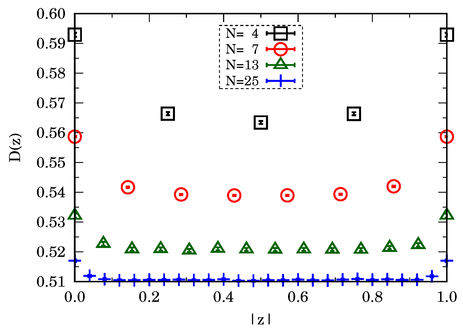
Figure 2.
Two-point-connected-function for , and . In our PIMC simulations we used Eqs. (4) and (5).
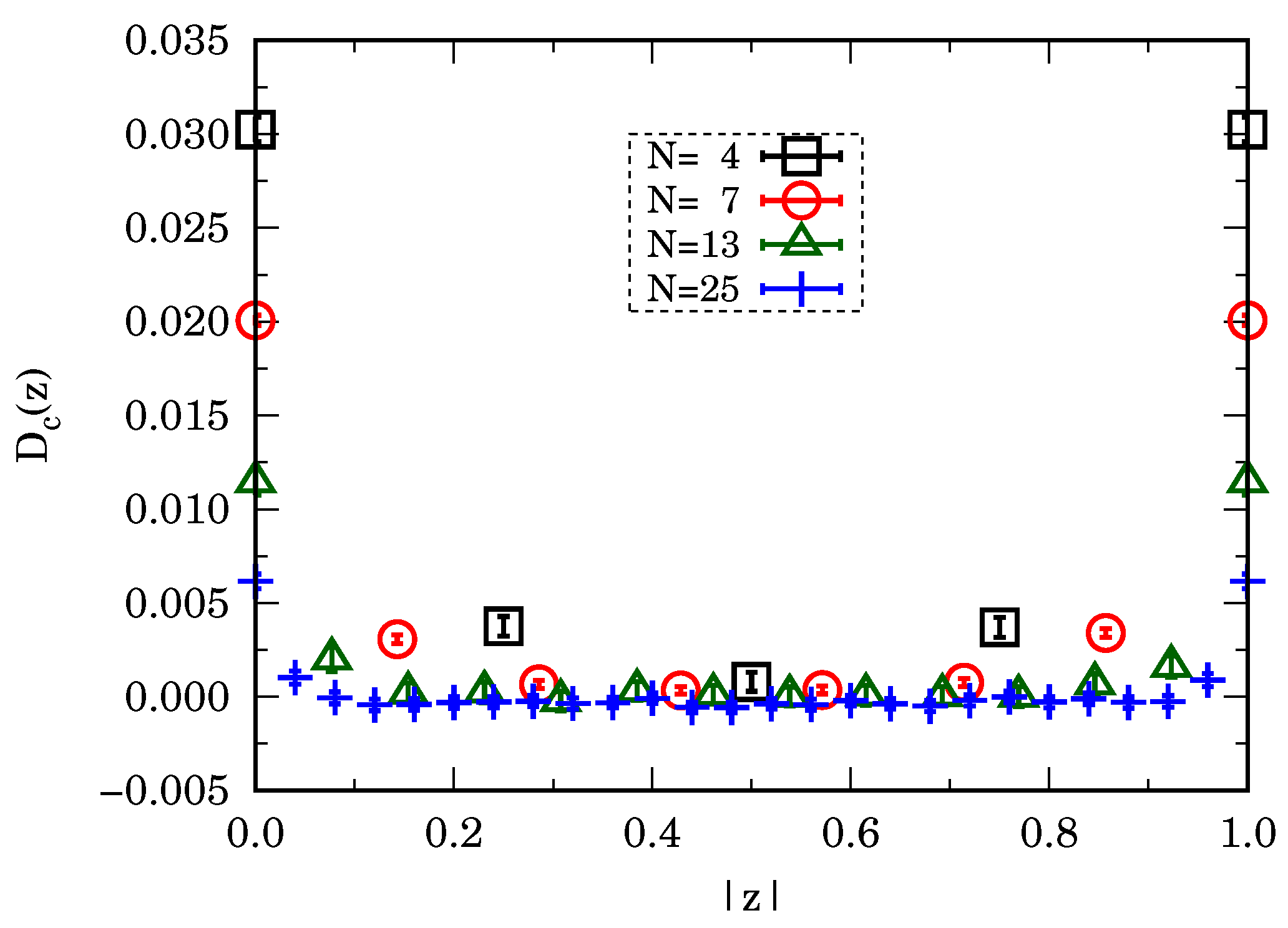
Figure 3.
Two-point-connected-function for , , and . In our PIMC simulations we used Eqs. (4) and (5).
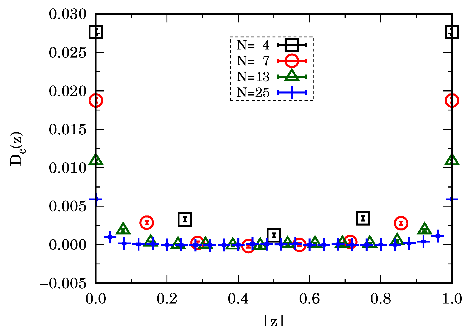
Table 1.
Renormalized mass , renormalized coupling constant , and one-point-value (vacuum expectation value of the field) for , and . In our PIMC simulations we used Eqs. (4) and (5).
| N | V | ||
|---|---|---|---|
| 4 | 0.1421(2) | 2.01178(2) | 0.7501(4) |
| 7 | 0.0602(1) | 2.001129(4) | 0.7339(2) |
| 13 | 0.0224(2) | 1.999894(5) | 0.7216(2) |
| 25 | 0.0084(1) | 2.000048(4) | 0.7148(3) |
Disclaimer/Publisher’s Note: The statements, opinions and data contained in all publications are solely those of the individual author(s) and contributor(s) and not of MDPI and/or the editor(s). MDPI and/or the editor(s) disclaim responsibility for any injury to people or property resulting from any ideas, methods, instructions or products referred to in the content. |
© 2023 by the authors. Licensee MDPI, Basel, Switzerland. This article is an open access article distributed under the terms and conditions of the Creative Commons Attribution (CC BY) license (http://creativecommons.org/licenses/by/4.0/).
Copyright: This open access article is published under a Creative Commons CC BY 4.0 license, which permit the free download, distribution, and reuse, provided that the author and preprint are cited in any reuse.