

Submitted:
25 December 2023
Posted:
26 December 2023
You are already at the latest version
Abstract
In the dynamic and complex environment of industrial control rooms, operators are often inundated with a multitude of tasks and alerts, which can lead to an overwhelming situation known as task overload. This state can precipitate decision fatigue and a heavier reliance on cognitive biases, potentially compromising the decision-making process. To mitigate such risks, the implementation of decision support systems becomes crucial. These systems are designed to assist operators in making swift and well-informed decisions, particularly when they sense their own judgment may be faltering. Our research introduces an AI-based framework that leverages dynamic influence diagrams and reinforcement learning to construct an effective decision support system. The cornerstone of this framework is the creation of a robust, interpretable, and efficient tool that supports control room operators during critical process disturbances. By integrating expert knowledge, the dynamic influence diagram forms a comprehensive model that captures the uncertainties inherent in complex industrial processes. It is adept at anomaly detection and recommending optimal actions. Moreover, this model is enhanced through a strategic partnership with reinforcement learning algorithms, which fine-tune the recommendations to be more context-specific and precise. The ultimate goal of our framework is to provide operators with a live, reliable decision support system that can significantly improve their response during process upsets. This paper outlines the development of our AI framework and its application within a simulated control room environment. Our findings indicate that the use of decision support systems can lead to improved operator performance and reduced cognitive workload. However, it also reveals a trade-off with situation awareness, which tends to diminish as operators may become overly reliant on the system’s guidance. Trust emerges as a critical factor in the adoption and effectiveness of decision support systems. Our research underscores the importance of balancing the benefits of decision support with the need for maintaining operator engagement and comprehension during process operations.
Keywords:
Decision Support Systems
; Control Room Operators
; Task Overload
; Artificial Intelligence
; Dynamic Influence Diagrams
; Reinforcement Learning
; Situation Awareness
; Trust in Automation
; Process Control
1. Introduction
This section establishes the context and scope of our research, followed by a comprehensive review of current literature in the field. We begin by outlining the dynamic landscape of industrial operations, emphasizing the crucial role and challenges faced by control room operators in modern, automated environments. Then, we transition to a detailed examination of recent scholarly work, assessing the advancements and applications of decision support systems within this domain, and identifying the gaps our research aims to fill.
1.1. Contextual Framework
In the rapidly evolving landscape of industrial operations, particularly in the energy sector, control room operators are pivotal in ensuring efficient and safe process management. Despite advancements in automation and process control technologies, these operators confront significant challenges in decision-making, often exacerbated by complex system interactions and high-stress scenarios. This study introduces an innovative AI-based decision support framework, employing dynamic influence diagrams and reinforcement learning, to address these challenges. Our approach presents a unique solution, enhancing decision-making effectiveness and accuracy in control room environments, thereby bridging a critical gap in existing operational strategies.
In the context of contemporary chemical processes, there’s a strong reliance on automation via Distributed Control Systems. Routine adjustments to expected process variations are overseen by Process Logic Controllers (PLC), which remotely control equipment components like valves and motor drives. At the core of industrial operations, operators interact with a Graphical User Interface (GUI) that aggregates and displays signals from instruments attached to machinery. Occasionally, system parameters might deviate beyond the set thresholds in the PLCs, triggering alarm notifications on the GUI. These alarms demand the operators’ discernment. Using the GUI’s data, operators are responsible for diagnosing the irregularity and deciding on the necessary actions to restore balance in the process. This diagnostic and corrective process demands intricate cognitive processing, urging operators to synthesize multiple data points, account for external factors like weather conditions, and predict the potential outcomes of each possible action [12]. Such situations can quickly become overwhelming for operators, making decisions susceptible to cognitive biases rather than comprehensive assessments. In these critical moments, the importance of decision-support tools becomes evident.
In this context, a broad definition of a decision support system (DSS) is given "as interactive computer-based systems that help people use computer communications, data, documents, knowledge, and models to solve problems and make decisions. DSS are ancillary or auxiliary systems; they are not intended to replace skilled decision-makers" [4]. The key advantage of decision support systems is their ability to handle and process large volumes of data in real-time.
1.2. Literature Review
The fusion of intelligent systems within manufacturing and the wider realm of operations management has traditionally been seen as a beneficial confluence of operational research (OR) and artificial intelligence (AI). This collaborative potential is underscored in studies by [1] and [2]. Additionally, [3] emphasized the escalating inclination towards the adoption of AI methodologies in this domain, particularly in their survey on DSS.
Decision support systems have been effectively developed for industrial applications, particularly in simulated studies. For instance, in [7], a DSS was crafted to identify abnormal operating procedures in nuclear power plant simulations. This innovation led to a marked reduction in decision-making time, improved performance, and a lighter workload. Further emphasizing advancements in the nuclear industry, [8] introduced a decision support system grounded in dynamic neural networks. This system adeptly guides operators by suggesting the appropriate procedures based on the system’s current state. DSS has also been extensively researched for broader industrial facilities, as highlighted in [11]. This particular study delves into the presentation of information to operators and the prioritization of alarms.
Bayesian networks have been used in fault detection, diagnosis, and prognostic in the industry but there are not many reported applications of Bayesian networks in the industry or only mentioned as knowledge-based systems as mentioned in [6]. In fault diagnosis, Bayesian networks can accurately identify the root causes of faults by considering the probabilistic relationships among observed symptoms and potential causes. An application of root cause analysis using Bayesian networks in manufacturing processes can be seen in [32]. In the study by [31], a versatile methodology for root cause analysis and decision support in industrial process operation is introduced. The approach has been effectively employed using both historical and simulated data. Bayesian networks have also been studied to answer the alarm flood predicament for control room operators [15].
One of the key points in the use of DSS is the human factor. The support is given to humans and it’s a person that will make the final decision. Those systems are not made to replace humans but to help them in their decision-making tasks. This aspect is one of the most important and difficult to consider since lots of human-related issues arise like trust, bias, and overload to name a few. Creating a model that processes a large amount of data and conveys the information in the most efficient way to an operator is not an easy task. DSS does not guarantee an increase in operator performance and needs to be carefully built [9]. Experiments on trust and operator bias using DSS have been done in [10]. It shows the complexity of the trust factor when an operator uses a DSS.
In this research, we build a framework to develop an efficient decision support system. This framework is based on a collaboration between a dynamic influence diagram (DID) and reinforcement learning (RL). We use a DID to efficiently model the uncertainty over time and provide the best decisions in this case. We use the local RL agent to precise the decision and provide the operator with the best possible procedure to solve any fault in the system. The effectiveness of our AI-based support system will be evaluated through a simulation in a control room setting. This evaluation will involve a comparison between groups utilizing the AI support and those without it, providing insights into the impact and efficacy of the system in operational contexts.
This paper is a combined and extended version of papers published in conferences about this experiment. See [30] for the construction of the dynamic influence diagram, [14] for the AI framework. In this paper, we commence by delineating the methodology employed, encompassing both the experimental design and the mathematical approaches utilized. Subsequently, we detail constructing a decision support system grounded in dynamic influence diagrams and reinforcement learning, along with the comprehensive framework we have developed. Following this, we present the application and evaluation of this framework through experimental testing, discussing the results and their implications. The paper concludes with a summary of our findings and reflections on their significance.
2. Materials and Methods
2.1. Digitised Screen-Based Procedures
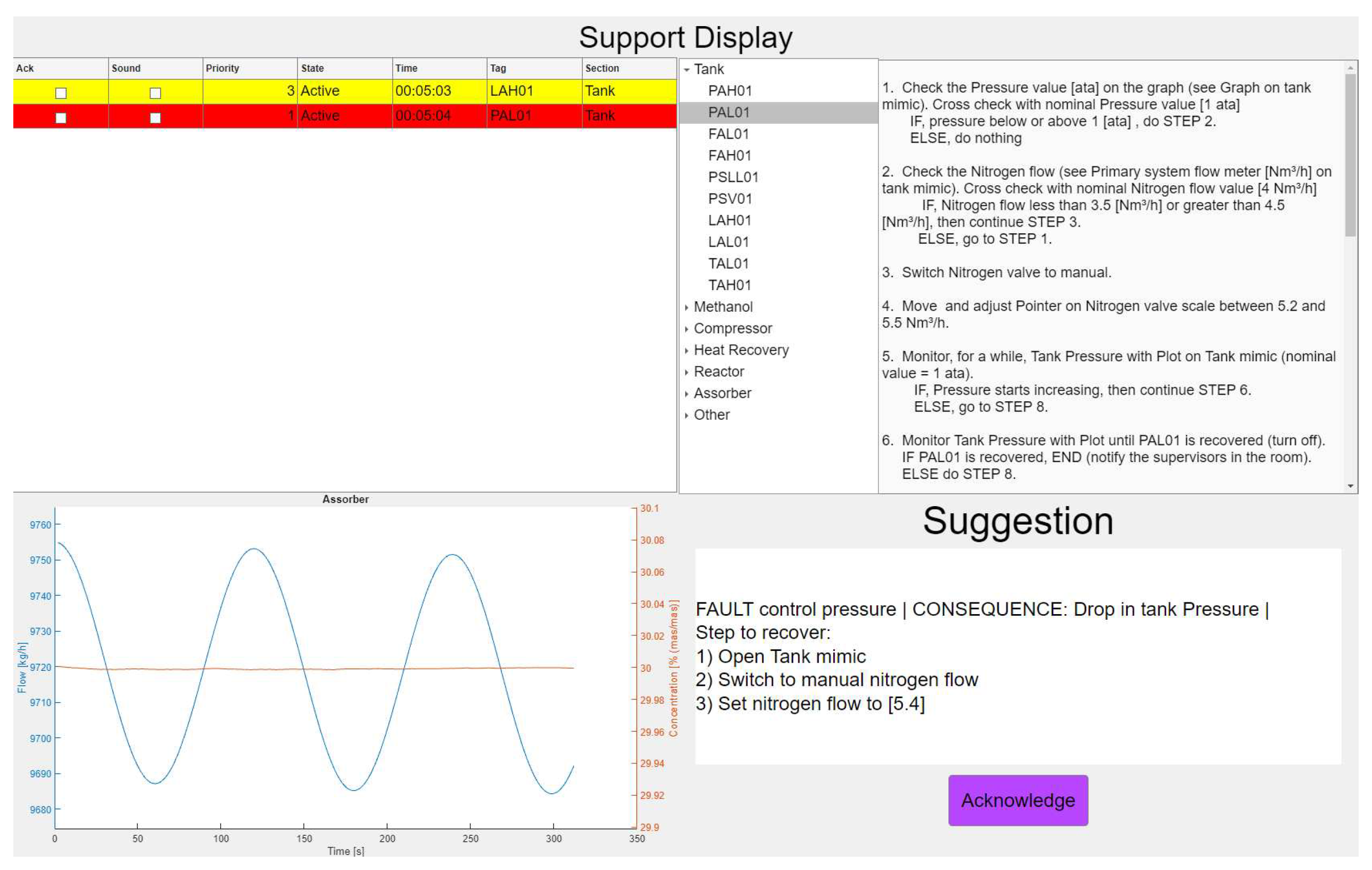
Procedures are of paramount importance to control room operators to ensure process safety. However, there are shortcomings in both the design and operator usage of these procedures. As a result, they have led to major accidents in safety-critical sectors like the nuclear and oil and gas sectors. For example, the Piper Alpha Platform explosion and the Longford Gas Plant 1 explosion and fire []. Procedure-related issues such as incompleteness, out-of-date, volume, or representation issues have led to different designs and updates, such as using computerized procedures or representations in flow charts. This study introduces a screen-based digitized procedure designed by [] to be compared with an AI-based procedure support. The digitized procedure was written in a hierarchical rule-based task representation format with detailed task steps to resolve each alarm in the plant. The procedure for each alarm was arranged for easy navigation on a support display as shown on the top right corner of Figure 3.
2.2. Experimental Setup
The foundation of our experiment is a simulator designed for formaldehyde production [5]. This simulator has been tailored to emulate the environment of a control room. A significant addition to this setup is the "support panel", which effectively transforms the simulator into a comprehensive control room simulation. This panel encompasses various features: a graphical representation for production monitoring, an alarm list, a procedure list, and an automated suggestion box. Regarding the process, the plant approximates a production rate of 10,000 kg/hr of 30% formaldehyde solution, generated via the partial oxidation of methanol with air. The simulator comprises six sections, namely: Tank, Methanol, Compressor, Heat Recovery, Reactor, and Absorber. With the inclusion of 80 alarms of varying priority levels, the simulator also accounts for nuisance alarms (irrelevant alarms). The simulator’s main screen is visible in Figure 1 and the detail tank mimic can be seen in Figure 3. To test the efficiency of our decision support, we created three scenarios:
- Pressure indicator control failure. In this scenario, the automatic pressure management system in the tank ceases to function. Consequently, the operator must manually modulate the inflow of nitrogen into the tank to preserve the pressure. During this scenario, the cessation of nitrogen flow into the tank results in a pressure drop as the pump continues to channel nitrogen into the plant.
- Nitrogen valve primary source failure. This scenario is an alternative version of the first one. In this case, the primary source of nitrogen in the tank fails. The operator has to switch to a backup system. While the backup system starts slowly the operator has to regulate the pump power to slow down the drop of pressure inside the tank.
- Temperature indicator control failure in the Heat Recovery section. The operator initially attempts to rectify the issue by manually adjusting the set point of the cooling water flow in the absorber. However, this intervention is ineffective. Consequently, the operator has to contact the supervisor for further guidance. The supervisor informs the operator that the fault is beyond the scope of control room resolution and requires the intervention of a field operator. While the field operator is dispatched to address the issue on-site, the control room operator is tasked with managing the reactor’s temperature. The primary concern in this scenario is the potential for the reactor to overheat. To mitigate this risk, the operator must closely monitor and adjust the cooling water temperature of the reactor.
Figure 1.
Process flow diagram of the Production. The formaldehyde is synthesized by combining methanol and compressed air, heating the mixture, initiating a chemical reaction in the Reactor, and finally diluting the solution in the Absorber to obtain the appropriate concentration. At the bottom is the different mimic that the operator can open on another screen for a process flow diagram of a specific part of the plant (see Figure 3).
Figure 1.
Process flow diagram of the Production. The formaldehyde is synthesized by combining methanol and compressed air, heating the mixture, initiating a chemical reaction in the Reactor, and finally diluting the solution in the Absorber to obtain the appropriate concentration. At the bottom is the different mimic that the operator can open on another screen for a process flow diagram of a specific part of the plant (see Figure 3).
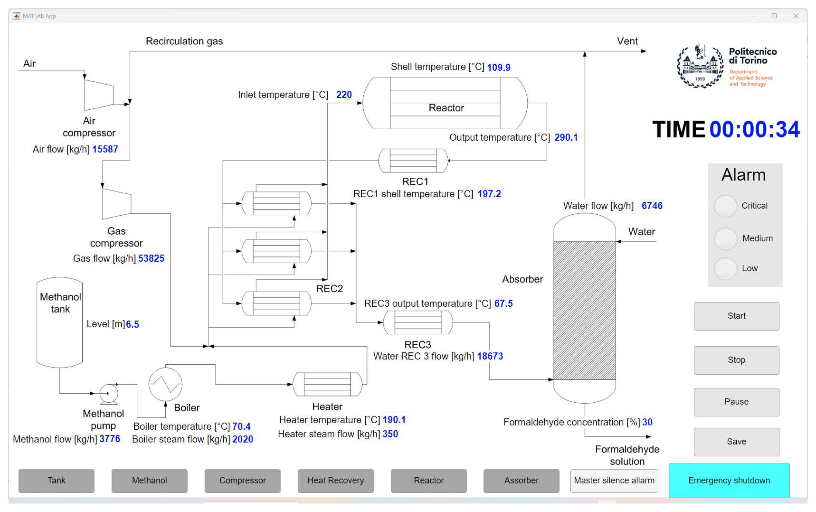
Figure 2.
Overview of the Tank section. On the left, we can see the nitrogen flow control panel. In the middle, is the process flow diagram of the tank with all the possible alarms. On the right is the graph of the physical value that needs to be monitored by the operator.
Figure 2.
Overview of the Tank section. On the left, we can see the nitrogen flow control panel. In the middle, is the process flow diagram of the tank with all the possible alarms. On the right is the graph of the physical value that needs to be monitored by the operator.
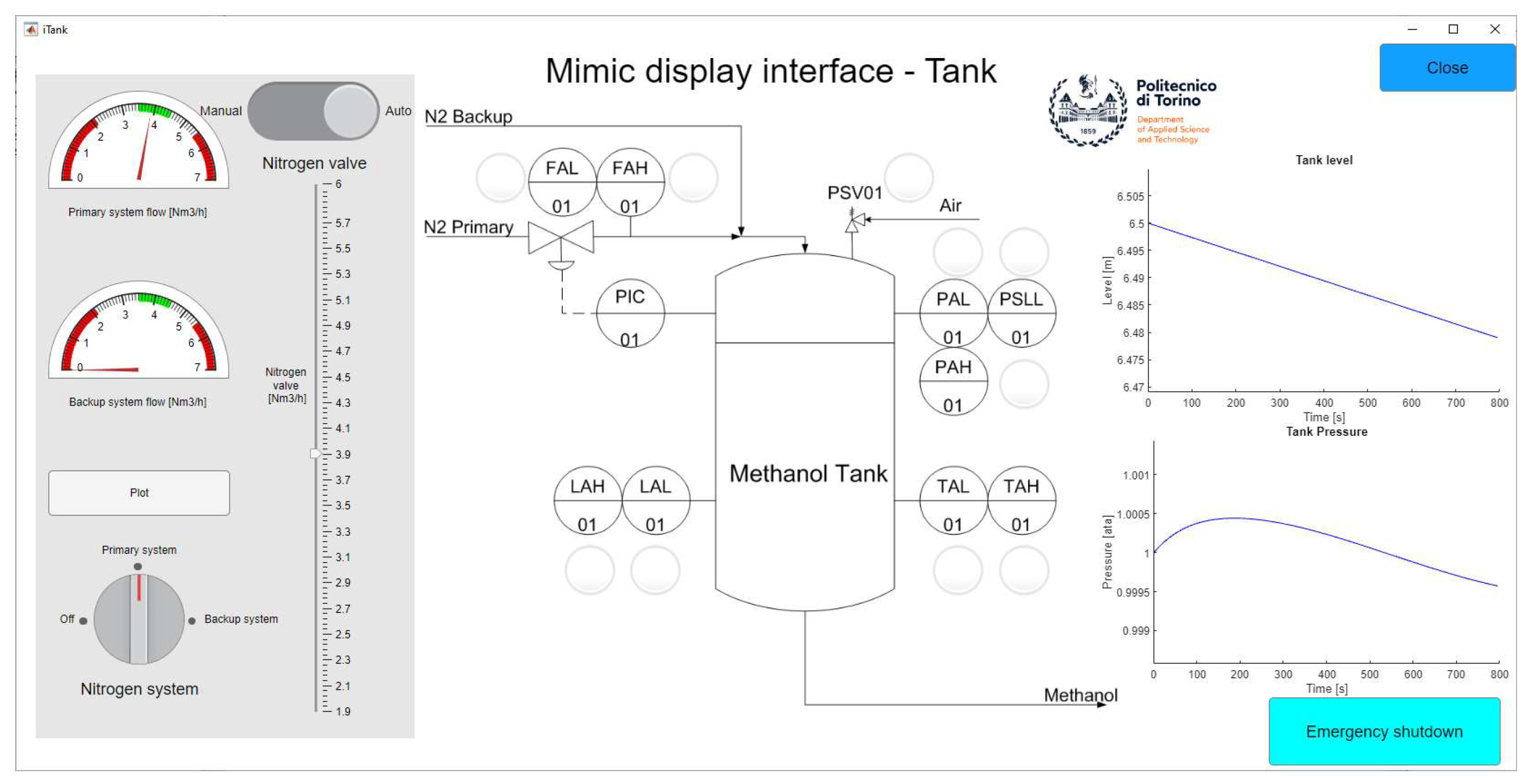
Figure 3.
Support Panel Layout: The upper left quadrant displays the alarm list, alerting the operator to current issues. The upper right is the traditional procedure system. The lower left features a critical graph related to production metrics. In the lower right, the suggestion box automatically provide situation-specific recommendations to the operator.
Figure 3.
Support Panel Layout: The upper left quadrant displays the alarm list, alerting the operator to current issues. The upper right is the traditional procedure system. The lower left features a critical graph related to production metrics. In the lower right, the suggestion box automatically provide situation-specific recommendations to the operator.
2.3. Dynamic Influence Diagrams
2.3.1. Influence Diagrams
An influence diagram is a graphical representation that depicts the relationships between variables in a decision problem [13]. It is a variant of a Bayesian network that incorporates decision nodes, chance nodes, and utility nodes to facilitate decision-making under uncertainty. Decision nodes represent choices or actions that can be taken, chance nodes represent uncertain events or states of the world, and utility nodes represent the preferences or values associated with different outcomes. Influence diagrams provide a structured framework for modeling and analyzing complex decision problems, allowing decision-makers to assess the expected utility of different choices and make informed decisions. A limited memory influence diagram is used to relax the perfect recall of the past and the total order of the decisions assumptions (see [13]). We define the discrete limited memory influence diagram as follows:
Definition 1.
Discrete limited memory Influence Diagram [13] A (discrete limited memory) influence diagram consists of:
- A DAG with nodes V and directed links E encoding dependence relations and information precedence.
- A set of discrete random variables and discrete decision variables , such that represented by nodes of G.
- A set of conditional probability distributions P containing one distribution for each discrete random variable given its parents .
- A set of utility functions U containing one utility function for each node v in the subset of utility nodes.
To identify the decision option with the highest expected utility, we compute the expected utility of each decision alternative. If A is a decision variable with options , H is a hypothesis with states , and is a set of observations in the form of evidence, then we can compute the probability of each outcome of the hypothesis and the expected utility of each action . The utility of an outcome is where is our utility function. The expected utility of performing action is
where represents our belief in H given . The utility function encodes the preferences of the decision maker on a numerical scale.
We use the maximum expected utility principle to make the best decision, meaning selecting an option such that
2.3.2. Dynamic Influence Diagram
Dynamic influence diagrams introduce discrete time to the model. The time-sliced model is constructed based on the static network, with each time slice having a static structure while the development of the system over time is specified by the links between variables of different time slices. The temporal links of a time slice are the set of links from variables of the previous time slice into variables of the current time slice. The interface of a time slice is the set of variables with parents in the previous time slice. A dynamic model can be seen as the same model put one after the other, each model representing the system state at a single time step and the connections from one time step to the next time step represent the influence of the past state of the system on the current state of the system as illustrated in Figure 4 [13]. In our experiment, we use a finite horizon dynamic influence diagram.
In Figure 5, we illustrate the structure of a basic dynamic influence diagram (DID), which is managed using the HUGIN software [16]. This diagram consists of several nodes:
- Decision Node (depicted in pink): This node represents the array of decisions options available to an operator at a point in time. Each state within this node has a direct impact on the distribution of physical values within the system, embodying the influence of operator decisions on the process.
- Physical Value Node: This node models the physical parameters of the system. However, rather than using precise values, the states are represented as intervals. This discretization approach is essential for simplifying the model while capturing the necessary detail. States indicating hazardous conditions in this node elevate the probability of adverse consequences.
- Consequence Node: This node encompasses the potential outcomes or consequences (e.g., tank explosion, tank implosion) that may arise from the system’s current state. Each state within this node is associated with a specific cost, reflecting the severity or impact of that outcome.
- Utility Node (colored in green): The utility node is where the cost (or reward) of each potential consequence is integrated. The utility value is computed by considering the probability of each consequence and its corresponding cost, thereby quantifying the overall risk or benefit associated with a particular system state.
- Physical Value Node with Stripes: This node represents the physical values from the previous time step. It is linked to the current physical value node to model the influence of past states on the present. Additionally, it is connected to the decision node to represent the operator’s ability to observe past physical values and make informed decisions in future time steps.
The overarching goal of this DID is to predict future physical values and utilize these predictions to guide the operator toward the most appropriate actions.
2.3.3. Conflict Analysis
An anomaly is identified when a variable deviates from its intended set point or the default value preordained by the automatic control mode. For the purpose of anomaly detection, we utilize conflict analysis as described in [13] within the influence diagram. Conflict in the influence diagram context is assumed when the evidence disseminated through the model exhibits inconsistencies or contradictions. Specifically, a conflict is assumed to arise when the product of the individual probabilities of each evidence exceeds the joint probability of all evidence. Consider a set of evidence, . We define the measure of conflict as follows:
A conflict is flagged if . Such conflicts can often be rationalized by a hypothesis, denoted by h, with a low probability of occurrence. If , it implies that h accounts for the conflict. In our model, h represents a fault within the system. Consequently, if a fault is capable of explaining a conflict, it is detected and identified as such.
2.4. Deep Reinforcement Learning (DRL)
In recent years, the integration of Deep Reinforcement Learning (DRL) techniques has revolutionized decision support systems, particularly in the realm of process control [22]. Process control involves the management and optimization of complex systems, where traditional control methods may fall short in addressing the complexities and uncertainties inherent in real-world processes. By leveraging the power of DRL, which combines deep neural networks with reinforcement learning algorithms, we aim to enhance the adaptability, efficiency, and robustness of decision-making in dynamic and uncertain environments.
DRL is a paradigm at the intersection of artificial intelligence, machine learning, and control systems [23]. It represents a powerful approach for training agents to make sequential decisions in complex and dynamic environments. At its core, DRL integrates deep neural networks to approximate complex functions and reinforcement learning algorithms to enable agents to learn optimal policies through interaction with their environment. Mathematically, the fundamental formulation of reinforcement learning involves the concept of Markov Decision Processes (MDPs), where an agent interacts with an environment by taking actions based on its current state, receiving rewards, and updating its policy to maximize cumulative future rewards. The Q-value function, denoted as Q(s, a), represents the expected cumulative reward of taking action ‘a’ in state ‘s’ and following the optimal policy thereafter. The Bellman equation, a cornerstone in reinforcement learning, expresses the recursive relationship between Q-values.
Twin Delayed Deep Deterministic Policy Gradient (TD3) Architecture:
One notable advancement in DRL is the Twin Delayed DDPG (TD3) architecture [24], designed to address challenges such as overestimation bias and brittle training. TD3 has been used in our framework as the base DRL architecture. TD3 incorporates twin Q-value estimators to mitigate overestimation errors and a delayed policy update mechanism for stabilizing the learning process. The TD3 algorithm introduces the following key equations:
Critic Update:
Policy Update:
Where:
- : expected cumulative reward for action a in state s.
- r: immediate reward obtained from taking action a in state s.
- : discount factor for future rewards.
- : maximum expected future reward in the next state .
- : Predicted Q-value by the target critic network.
- y: Target value for the critic update,
- : state, action, reward, and next state, sampled from replay buffer.
- : Action selected by the target policy in the next state.
- : Q-value associated with the selected action and state.
- : Action selected by the policy in the current state.
These equations encapsulate the optimization objectives for updating the critic and policy networks within the TD3 architecture, providing a solid foundation for understanding its theoretical underpinnings and subsequent practical implications in the context of process control decision support systems.
2.4.1. DRL for Process Control
Authors in [20] have focused on the use of DRL in the process control environment. The following state, action, and reward are formulated in our case following the literature [22].
State:
In the context of a Partially Observable Markov Decision Process, relying solely on the observed state may be inadequate due to the system’s inherent partial observability constraints. Consequently, the state perceived by the DRL system differs from the actual environment state. To overcome this challenge, the investigation employs a tuple comprising the history of expert actions concatenated with the history of process variables. This history can extend up to a length denoted as "l," as illustrated in eq. (8). The selected historical information encompasses the current state at time "t" and only the preceding trajectory at time "t - 1".
Action:
The actor-network in reinforcement learning is responsible for determining the policy, which is essentially the mapping from states to actions. In the context of the TD3 architecture, the actor network typically outputs a continuous action parameterized by a neural network. The actor’s output can be denoted as follows:
Here, is the deterministic policy function, representing the mean of the distribution over the continuous action space.
Reward:
In a disturbance rejection scenario, the agent aims to determine an optimal policy, denoted as , which effectively minimizes tracking error and stabilizes the process while deviating minimally from the optimal set-point. This objective is realized by incorporating the goal into the DRL agent through a reward function (r) or a cost function (-r), such as the negative l1-norm of the set-point error. Mathematically, for a system with "m" process variables as inputs, this is expressed in eq. (10).
2.4.2. Specialized Reinforcement Learning Agent (SRLA)
The challenge in implementing DRL within complex and continuous state-action spaces, like those found in real-world processes with multiple input variables, lies in the model’s tendency to learn from the entire dataset rather than focusing on relevant data. This can pose difficulties in achieving convergence. Authors in [17,18] have formulated a framework called Specialized Reinforcement Learning Agent (SRLA) which specialized the DRL agent on particular required states such as abnormalities to reduce the task complexity and activating the agent for training and inference only when it is most required. The framework proposes a hierarchical architecture composed of a higher probabilistic model and a DRL agent at the lower level of the hierarchy. The probabilistic model defines the states of specialization and the DRL agent is activated on those states for training and inference as shown in Figure 6 taken from [17].
SRLA in Process Industry:
Authors in [19] have applied an instantiation of SRLA in process control simulation that outperforms conventional methodologies, and therefore, we have defined a similar structure to use as our AI framework.
3. Statistical Test
In this study, we use statistical tests to assess the significance of the result obtained. We initially conducted the Shapiro-Wilk test [25] to assess the normality of the data. This test is crucial in determining the subsequent statistical tests to be employed. When data showed equal variances, as confirmed by Levene’s test [27], we used the Student’s T-test [29] to compare the means of the groups. In cases where equal variances were not observed, we opted for Welch’s T-test [28]. Additionally, the Wilcoxon Rank-Sum Test [26] was utilized in situations where the normality assumption was not met, making it an apt choice for comparing two independent samples with non-normal distributions.
4. Result
4.1. Construction of the Model
In this section, we provide a detailed explanation of the process involved in constructing the dynamic influence diagram. This diagram can be seen in Figure 7 and Figure 8. The primary objective of this model is to detect anomalies and offer the operator an optimal procedure to follow. The simulator is not publicly available but the models and the code to use the model are available at https://github.com/CISC-LIVE-LAB-3/Decision_support
4.1.1. Operational Framework and Objectives of the DID Model
The DID constructed for this research is tailored to address the three scenarios delineated in section 2.1, with a particular focus on the tank system within the process. For the initial two scenarios, the DID provides substantial decision support by simulating the tank system’s physical processes, thereby guiding operators toward maintaining systemic equilibrium. The model’s primary objective is to balance the nitrogen injection rate and the pump power, thereby preventing the risks associated with both overpressure (explosion) and underpressure (implosion). By doing so, the DID facilitates the maintenance of optimal pressure levels inside the tank, which is crucial for the plant’s stability and operational efficiency.
However, for the third scenario, the complexity of modeling the entire process was deemed impractical within the scope of this work. Instead, a simplified model was developed specifically to provide decision support for this scenario. While this streamlined model does not encompass the full intricacies of the process, it is designed to effectively detect anomalies and assist the operator in making the necessary adjustments, particularly concerning the reactor’s temperature. This approach ensures that the operator receives targeted and relevant guidance, enabling them to respond to the scenario with appropriate actions without the need for a comprehensive model of the entire system.
4.1.2. Fault detection
Fault detection in our system is carried out through conflict analysis, as explained earlier. The models for detecting faults in the first two scenarios and the last scenario are illustrated in Figure 9 and Figure 10, respectively. Both models function in a similar manner, but in the first two scenarios, there are additional elements like the "System" node and "Pressure T+1". These elements indicate the option to switch to a backup system in scenarios 1 and 2, which adjusts the nitrogen flow based on the pressure readings.
In both models, the default setting is the auto mode with a predetermined flow. A fault is indicated when the actual flow is anomalously low, leading to a conflict between the expected and actual flow readings. To resolve this, the "Fault" node is adjusted to "Fault control", aligning the low nitrogen flow with the fault condition and thus resolving the conflict. If the issue continues even after reverting to auto mode, a new conflict arises, which is then resolved by adjusting the fault value Fault valve".
4.1.3. Parameter and Structure Specification
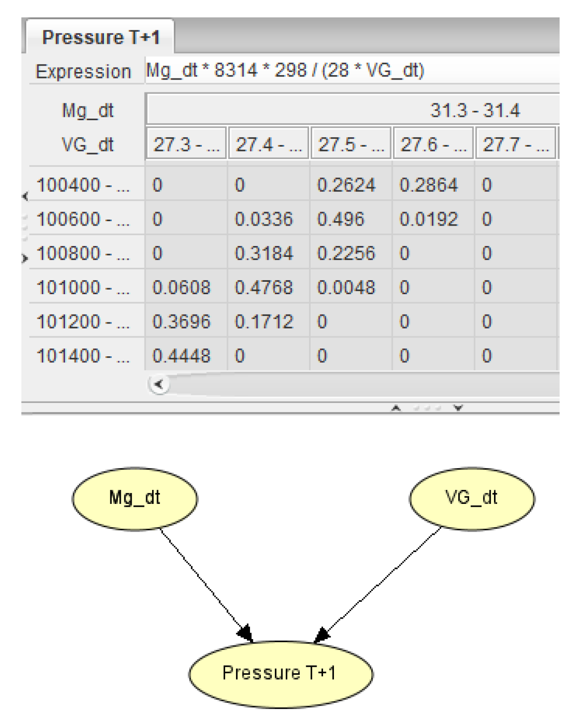
The parameter specification relies on these physical equations related to the process as outlined in [5] and the logic of the model. Owing to the discretization of the variables, we utilize a sampling technique to formulate the resultant Conditional Probability Table (CPT). To demonstrate this methodology, we consider the calculation of pressure from our case study.
The pressure is contingent on two variables, Mg (mole) and VG (), abiding by the perfect gas law:
In our experiment, the corresponding physical equation is:
where P is expressed in Pascal, MG in Kg, and VG in . The temperature, 298, is in degrees Celsius, 8.314 J/(mol*K) is the perfect gas constant, and 28 is the molecular mass of methanol (kg/kmol), which is divided by 1000 to convert to (kg/mol).
We build the structure of the model according to the formula. The pressure depends on Mg and VG. We link them to the Pressure node. We also use this formula to set the expression in the pressure node. The graph can be seen in Figure 20. Additionally, it is worth mentioning that Mg and VG serve as intermediate variables in order to avoid directly connecting all variables to the pressure node, which would result in a too-large conditional probability table. It has also the benefit of displaying the model of the different physical equations in a comprehensible way.
For the CPT generation, we employed a sampling method. In our study, we generate 25 values within each interval for the parent nodes Mg and VG. We then calculated the probability of a value falling within the "Pressure T+1" state intervals after applying the relevant formula. This methodology of sampling and probability estimation is similarly applied to other nodes like Mg, VG, Level of Liquid, Flow of Liquid, Intermediate Node, and Temperature of the Reactor, each governed by their respective physical equations.
The CPT for "Nitrogen Flow" and "Pump Power" depend on the state of their parent nodes. For example, if the system is in "Auto" mode without any faults, the "Nitrogen Flow" is typically around 3.9–4m3/h. This is a normal range for when the system automatically controls the flow to work best. The "Pump Power" also changes based on its parent nodes. These logical CPTs help the Bayesian network to mimic the system’s behavior in different situations, making it a useful tool for decision-making and predicting future scenarios.
Figure 11.
Exemple for the calculation of the Pressure CPT.
4.1.4. Utility
In our model, we use nodes to represent possible outcomes, such as incidents that could occur in the industrial plant. After inputting observed values and decisions into the influence diagram, we calculate the chances of these outcomes. Each outcome, or consequence node, is linked to a utility node that shows the financial cost of that outcome. For example, the cost of a tank explosion might be around one million dollars, based on sources like [5]. The likelihood of such an explosion depends on factors like pressure and flow rates, and every decision made in the model affects these probabilities.
The model specifically addresses outcomes related to tank pressure, such as "Tank explosion" and "Tank implosion." These are directly linked to pressure changes. For example, the chance of a tank explosion increases linearly as pressure rises. If the pressure is in a safe range, say "101200-102600" Pa, the explosion risk is zero. But if it drops below a critical point, like "-inf-96800" Pa, the explosion risk becomes certain. The "Tank implosion" risk works similarly but increases as pressure drops. This setup helps predict and manage the risks associated with pressure changes in the tank.
4.1.5. Dynamic Model
We use a DID in our model to predict future states of the system and identify actions that maximize utility at each moment. This approach ensures that the chosen actions are optimal, taking into account both current and future scenarios. The model operates across 10 time steps, with each step representing one minute. This allows the model to project the system’s state in one-minute intervals for the next 10 minutes, effectively capturing the dynamics of the system. Such a setup enables us to inform the operator about potential critical events in the next 10 minutes and suggest the best course of action to prevent or manage these events.
In our model, decision-making is closely linked to the states of various nodes, such as "Auto" and "Set Point," which are influenced by the current pressure ("T_Pressure T+1"). This setup mimics how an operator would make decisions based on current and future pressure states, enhancing the model’s realism and predictive capability. The DID is designed to model scenarios where the operator makes correct decisions based on this information. The model also establishes a cause-and-effect relationship between the "Auto" and "Set Point" nodes, where the "Auto" mode automatically sets the "Set Point" to a specific value. This is essential for modeling the system’s response to different operational modes and affects the range of possible actions and their outcomes. Overall, the model provides a detailed representation of the decision-making environment, considering various factors like current conditions, future projections, and the balance between automated and manual controls. This comprehensive approach makes the DID a powerful tool for simulating and enhancing decision-making in complex systems.
4.2. AI Framwork
In the proposed framework, we integrate the predictive prowess of a dynamic influence diagram (DID) with the adaptive capabilities of Reinforcement Learning (RL) agents. The DID is meticulously constructed upon the physical equations governing the process, with a focus on the dynamics of the tank system and other relevant components for specific scenarios. This model is not only designed to capture the physical dynamics of the tank system but also to account for uncertainties inherent in the process. It is adept at identifying anomalies, representing fault states of the tank, forecasting future states, and recommending optimal actions.
A pivotal aspect of employing Bayesian networks, such as the DID, is the discretization of variables, as influence diagrams typically perform more effectively with discrete variables. To address the limitations posed by discretization, we employ localized reinforcement learning agents. These agents refine the actions suggested by the DID, providing continuous values instead of broad intervals. This precision aids the operator in making more accurate decisions.
However, safety concerns necessitate a cautious approach when integrating black-box models like RL agents. Therefore, the continuous value suggested by an RL agent is only utilized if it falls within the DID-recommended interval. If the RL-derived value is outside this interval or appears contradictory, the DID’s recommendation is prioritized by default. This approach ensures that the system’s recommendations remain within safe operational parameters, leveraging the strengths of both the DID and RL agents to enhance decision-making while maintaining a safety-first perspective.
It operates within the Human-in-the-Loop (HITL) setting, employing a Multi Specialized Reinforcement Learning Agent (M-SRLA) configuration. Within this setting, multiple agents operate independently, and only a designated agent becomes active to propose the optimal control strategy to the operator when a process abnormality is identified through the influence diagram, as illustrated in Figure 12, taken from [21]. This framework is called "Human-Centered Artificial Intelligence for Safety-Critical Systems" (HAISC).
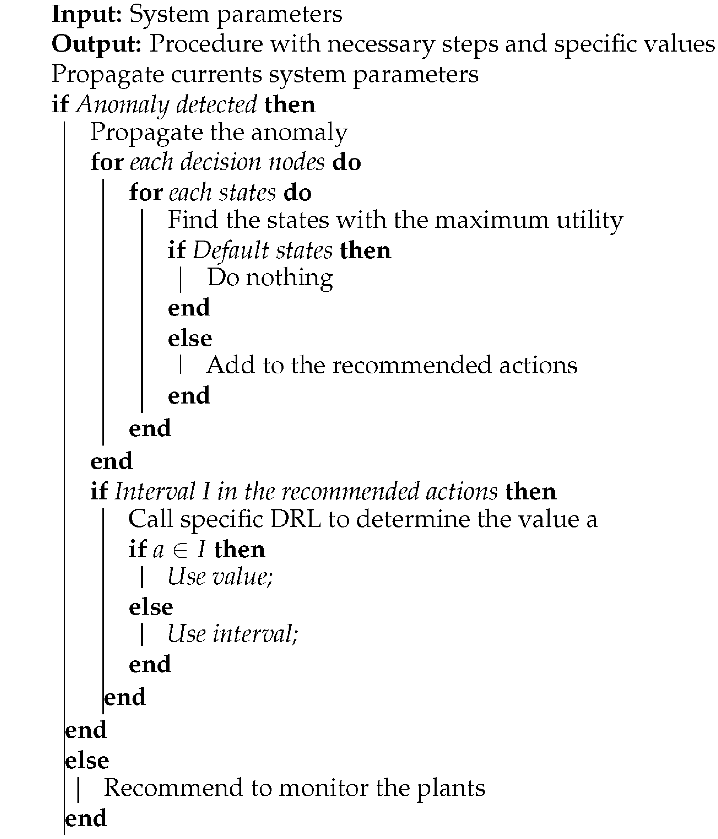
| Algorithm 1: Influence Diagram-based Recommendation Algorithm. |
 |
4.3. Use of the Model
The model is used to detect anomalies and propose the optimal set of actions for the operator. We can separate the use of the model into 4 different steps:
- First, we use the anomalies detection model to detect potential faults in the system.
- Next, we incorporate both the observed data at T0 and the potential anomaly identified in the previous stage. We then evaluate various actions at T1 for their maximum utility, thereby formulating an optimal set of actions intended to either prevent or mitigate a potentially critical event.
- If some set point in the form of an interval is recommended to the operator, the appropriate reinforcement learning agent is called to precise this value.
- Finally, the operator is presented with the optimal procedure, which outlines the recommended course of action based on the preceding analyses. The fault is also provided to the operator with its potential consequences,
efinition
Scenario 1.
In the first scenario of our study, an issue arises with the nitrogen flow being lower than expected due to a malfunction in the automatic control system. As a consequence, the pressure is also below the normal range. The evidence of node "Auto" being in the state "on" creates a conflict with the nitrogen flow value since, in auto mode, the flow of nitrogen should be higher. By setting the "Fault" node to the state of "control valve failure," the conflict is resolved. At this stage, the model represents the current state of the system, considering the failure. Upon analysis, it is found that switching the "Auto" mode to the state "off" and manually adjusting the set point of the nitrogen flow to a value between 4-7 are the actions with the maximum utility. At this point, the reinforcement learning agent is called and proposes the value 5.6 which is in the interval recommended by the DID. These actions and the set point are then recommended to the operator with the indication of the failure.
Scenario 2.
In the second scenario, we encounter a complication with the nitrogen flow, which is registering lower than expected. This anomaly is attributed to a fault in the primary system’s flow control. Initially, the model is unable to distinguish whether the issue stems from the automatic system or the primary system. The "Auto" node being in the "on" state suggests that the nitrogen flow should be higher. A conflict is detected between the auto mode and the nitrogen flow.
To address this, the "Fault" node is set to "control valve failure," which reconciles the conflict in the model’s first iteration. However, after 10 seconds, the model is re-evaluated, and the issue persists, indicating a conflict between this time the expected set point and the actual nitrogen flow. At this point, the fault is identified as a "Fault primary system," and the model advises switching to the backup system. The transition to the backup system has a lead time of two minutes, during which the flow is set as "0-1.5".
To mitigate the pressure drop during this interval, the model suggests a reduction in pump power. This adjustment is carefully calibrated to slow the pressure decline without significantly affecting the nitrogen concentration within the system. The set point is found using the reinforcement learning agent for the pump power after checking it with the interval recommended by DID. Once the pressure stabilizes within the desired range, the model then recommends reactivating the pump power to its automatic setting, thereby resuming normal operations. This sequence of recommendations ensures that the system maintains its functionality while addressing the fault, minimizing disruption to the process.
Scenario 3.
In the third scenario, the decision support system encounters a conflict between the "Auto" mode and the water flow in the absorber. Despite the system’s recommendation to switch to manual operation and adjust the set point, the problem persists. A fault is detected and the system advises the operator to "call supervisor."
The supervisor’s role is to acknowledge the issue, which is beyond the scope of control room operations, and to dispatch a field operator to address the problem directly. Meanwhile, the control room operator is instructed to concentrate on monitoring the reactor’s temperature to prevent any extremes of overheating or undercooling.
Should the reactor temperature reach an abnormal level, the decision support system promptly provides the operator with the precise adjustment needed for the cooling water system’s temperature setting using the third RL agent after checking the value with the interval recommended by DID. This guidance is crucial for maintaining the reactor’s temperature within safe operational limits and ensuring the continuity of the production process while the field operator resolves the underlying issue.
By utilizing this approach, we employ a single model to evaluate the current state of the system, forecast future states, and suggest the optimal procedure for the operator. It is crucial to emphasize that these procedures are continuously updated and can adapt to system changes. This framework provides a solid foundation for developing efficient procedures. Those procedures presented to the operator are shorter compared to the standard procedure as they focus solely on the necessary action. A classical procedure consists of troubleshooting, action, and monitoring phases. The decision support system assists the operator in decision-making without replacing the initial procedure. Instead, it complements the existing procedure by offering recommendations in difficult situations. This approach offers a comprehensive solution, enhancing operators’ decision-making processes and ultimately improving overall system performance.
5. Experiment
In the experiment, two groups were established: Group 1 (G1), which operated without the decision support system, and Group 2 (G2), which utilized the decision support system. Both groups were subjected to the same three scenarios for testing. Subsequently, their performances and responses were compared to assess the impact of the decision support system.
5.1. Participants
A group of 50 volunteer participants, primarily composed of students, took part in this study. 23 in group 1 and 25 in group 2. These participants represented a range of experience levels, with the majority being master students in Chemical Engineering. In Figure 13 we can see the experimental setup.
5.2. Situation Awareness
Situation awareness (SA) is evaluated through a two-pronged approach. Firstly, participants complete the Situation Awareness Rating Technique (SART) questionnaire following each scenario. This self-assessment tool measures the quality of the participant’s awareness of the situation, capturing their ability to monitor, comprehend, and project the status of various elements in the environment.
Secondly, the SA of participants is assessed in real-time during the scenarios using the Situation Present Assessment Method (SPAM). This method involves intermittently querying participants with three targeted questions at different stages of the scenario. These questions are designed to gauge the participants’ attention and understanding of the current state of the system, their projection of future states, and their perception of situational complexity and dynamics. This dual approach allows for a comprehensive assessment of SA, combining reflective self-reporting with in-the-moment evaluations.
The result of the SART questionnaire can be seen in Figure 14. The statistical test Table 1 shows no statistical significance between the two groups.
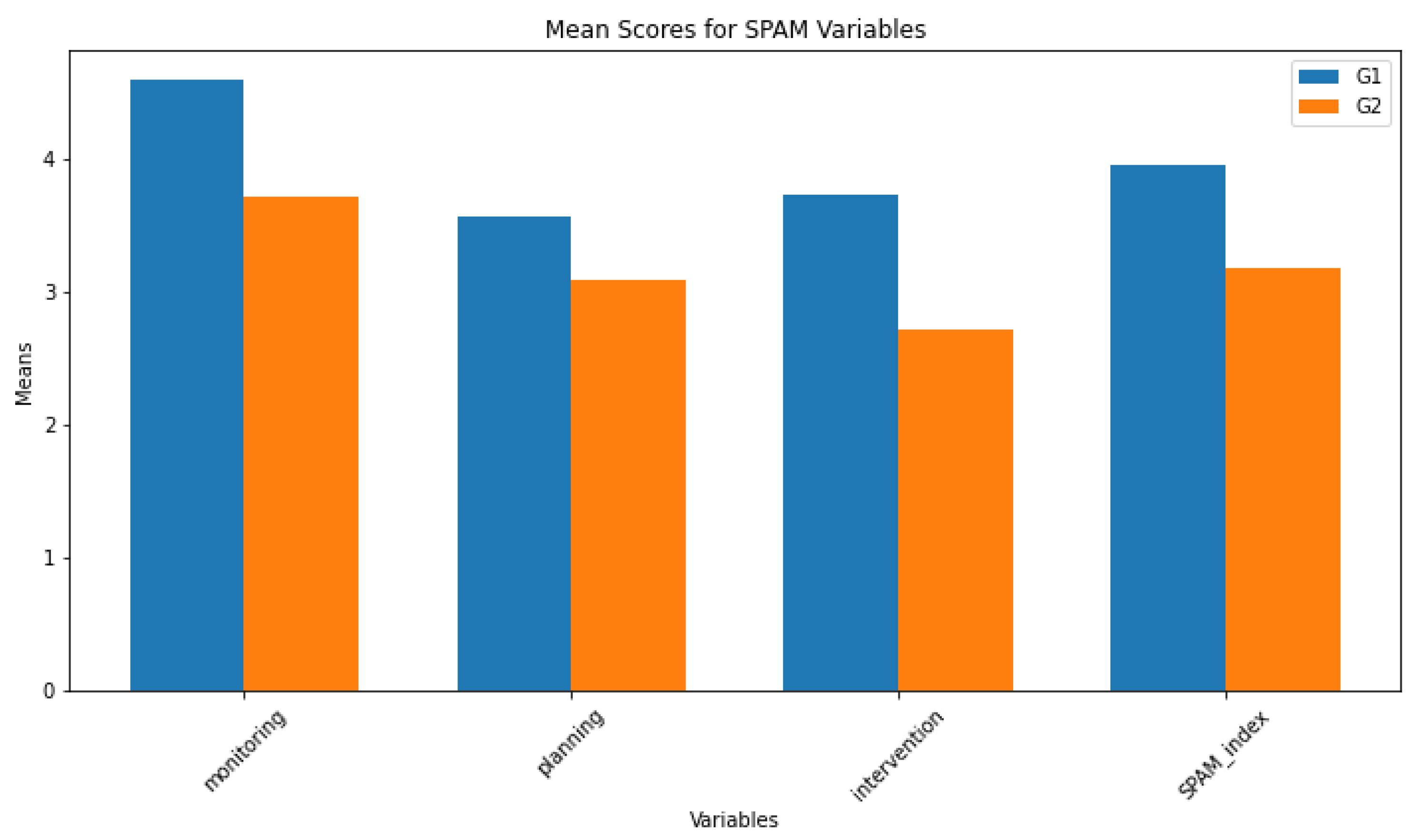
Based on the results presented in Table 2, and noting that Group G2 consistently shows lower values than Group G1 Table 2, we interpret the data as follows:
-
Monitoring:
- –
- The Shapiro-Wilk test indicates non-normal distribution for G1, but normal for G2.
- –
- Significant differences in monitoring are observed, with G4 showing lower levels as indicated by the t-test and Wilcoxon Rank-Sum Test.
-
Planning:
- –
- Both groups exhibit normal distribution according to the Shapiro-Wilk test.
- –
- No significant differences in planning, though G2 tends to have slightly lower levels.
-
Intervention:
- –
- Shapiro-Wilk test suggests borderline normal distribution for both groups.
- –
- A significant difference is found, with G2 engaging in less intervention than G3.
-
SPAM Index:
- –
- Normal distribution is suggested for both groups by the Shapiro-Wilk test.
- –
- The SPAM Index shows a significant difference, with G2 having a lower index than G3.
In summary, Group G2 consistently exhibits lower levels of monitoring, intervention, and overall SPAM Index compared to Group G1. While planning shows no significant difference, the trend of lower values in G2 is consistent across other dimensions.
Figure 15.
Bar plot of the variable of the SPAM questionnaire for the two different groups. G1 without decision support and G2 with.
Figure 15.
Bar plot of the variable of the SPAM questionnaire for the two different groups. G1 without decision support and G2 with.
5.3. Workload
Workload among participants was quantitatively assessed using the NASA Task Load Index (NASA TLX), a widely recognized subjective workload assessment tool. Participants completed the NASA TLX form after each scenario, which evaluates six dimensions of workload: mental demand, physical demand, temporal demand, performance, effort, and frustration level. The TLX index is the average of those variables. The bar plot can be seen in Figure 16 and the statistical test in Table 3. The analysis of these results reveals the following insights:
- Mental Demand: The statistical tests indicate no significant difference in mental demand between groups G1 and G2.
- Physical Demand: Similarly, there is no significant difference in physical demand between the groups.
- Temporal Demand: The results show no significant difference in temporal demand, suggesting both groups experienced similar time-related pressures.
- Performance: No significant difference in perceived performance is observed between the groups.
- Effort: The effort levels do not differ significantly between the groups.
- Frustration: A significant difference in frustration levels is observed, with G1 experiencing more frustration than G2.
- TLX Index: The overall TLX Index, representing the combined workload, shows no significant difference between the groups.
In summary, while the groups show no significant differences in mental demand, physical demand, temporal demand, performance, and effort, there is a notable difference in frustration levels. This suggests that while the overall workload may be similar, the qualitative experience of the workload, particularly in terms of frustration, differs between the groups. The group with the decision support (G2) show a lower level of frustration.
5.4. Performance
This section details a few performance metrics derived from operational data to compare the two groups’ performance. The metrics presented here include reaction time (this is the time it takes to switch the nitrogen valve button from Auto to Manual depending on the scenario and initial task as written in the procedures) and response time (the time it takes to act. For example, in Scenario 1, this means the time it takes to adjust the nitrogen valve scale to the correct value) and the overall performance of the operators (this considers the time it takes to recover the low-pressure alarm or, in some cases, those who fixed the fault even before an alarm. Those below or equal to the (25th) percentile are grouped as "optimal performance." Those who fall below or equal to the (50th) percentile are classified as ’good’, and the rest as ’poor performance’). The analysis used data collected from 21 participants in each group ( and ).
Figure 17 shows their overall performance comparison for the three scenarios. Table 2 compares each scenario with the reaction time and the response time. A nonparametric test, the Mann-Whitney U test (), was used to check the significant difference between the groups in each scenario based on their performance.
- Reaction time/Response time/Overall Performance: Based on the overall performance, Group 2 had optimal performance compared to Group 1 Table 4. This is typically the same for the reaction and response times. The statistical tests Table 5 indicate significant differences in the two groups’ time-based and overall performance metrics while solving the scenarios. Except scenario 3 where there is no significant difference between the two groups. One possible interpretation is the wide range of different behaviors inside each group due to the complexity of the task. All in all, the group with the decision support showed better performance than the group without.
5.5. Physiological Data
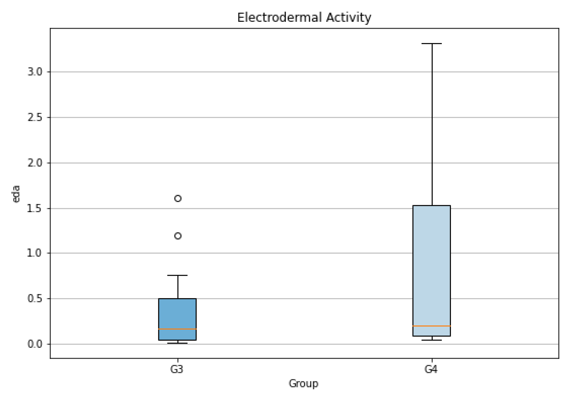
In this study, we conducted an extensive quantitative analysis of physiological metrics collected using smartwatch technology. Our focus was on three key parameters: heart rate, temperature, and electrodermal activity (EDA). The aim was to identify significant differences across groups and to uncover underlying patterns and variations within the data. Such insights are invaluable for understanding the physiological responses as captured by the wearable device.
For this analysis, we examined data from Group 1, consisting of 14 participants, and Group 2, with 17 participants. Each participant’s mean values for heart rate, temperature, and EDA were calculated across various scenarios. This methodology enables us to assess and compare the average physiological responses of the groups to these scenarios, shedding light on the distinct patterns observed via the smartwatch.
The Table 6 presents the outcomes of our statistical tests across heart rate, temperature, and EDA. For heart rate, although both groups G1 and G2 pass the normality test, a significant difference in variances is detected. The Welch’s T-test indicates a borderline significant difference (p-value = 0.05), a finding echoed by the Wilcoxon test (p-value = 0.09). The temperature measurements didn’t show any significant difference between the two groups. For EDA, neither group shows a normal distribution. The variance is not significantly different, and the Wilcoxon test suggests no significance in their differences.
A notable finding was observed in the comparative analysis of groups G1 and G2. It was discerned that Group 2 tended to have a lower heart rate than Group 1. This outcome is particularly significant as it suggests the potential influence of a recommendation system in alleviating stress among control room operators. The implication is that decision support systems may play a crucial role in reducing stress levels, thereby potentially improving both the well-being and operational efficiency of operators in high-stress environments. Such findings underscore the importance of integrating supportive technologies in workplaces where decision-making under pressure is a regular occurrence.
Figure 18.
Box plot of the Heart Rate Across Three Scenarios for Each Group.
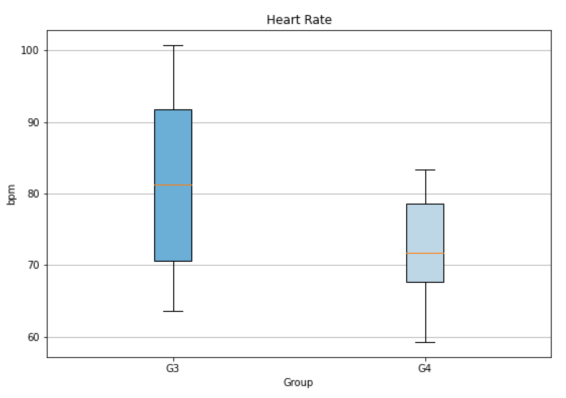
Figure 19.
Box plot of the Temperature Across Three Scenarios for Each Group.
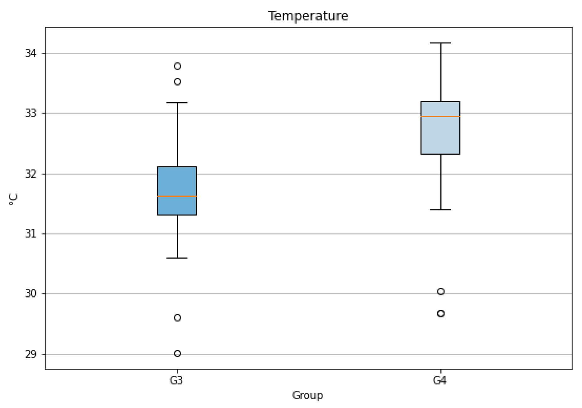
Figure 20.
Box plot of the Electrodermal Activity Across Three Scenarios for Each Group.
6. Discussion
The implementation of a decision support system appears to reduce operator workload, as evidenced by the results of the NASA TLX questionnaire and observed decreases in heart rate. These findings suggest that decision support can be beneficial for control room operators, enhancing their efficiency. Additionally, there is a noticeable improvement in performance; operators respond more rapidly and are more likely to resolve issues when utilizing decision support. However, it’s important to note that the use of decision support systems may also lead to a decrease in situation awareness. This is indicated by the results of the SPAM methodology. Therefore, it’s crucial to employ decision support systems judiciously, balancing the benefits of reduced workload and increased performance with the potential impact on situation awareness.
Decision support systems are not intended to supplant the critical thinking skills of operators but rather to augment their decision-making capabilities in high-stress or complex situations where human cognitive limitations might hinder optimal outcomes. The deployment of decision support is most beneficial in scenarios where operators acknowledge the limits of their expertise or when faced with information overload. Additionally, decision support systems can serve as valuable educational tools for novice operators. They can act as a virtual mentor, guiding less experienced personnel through the decision-making process in simulated or low-risk environments. This can foster confidence and reinforce the learning of best practices.
Another significant aspect of utilizing the framework is its capability to extract and present a wide range of critical information. This includes indicators of proximity to alarm thresholds, predictions of the likelihood and timing of potential events, and associated probabilities. Given that the model encompasses the process dynamics, it can access and utilize a wealth of additional data. However, it’s crucial to balance the amount of information presented to the operator. While the Decision Influence Diagram (DID) framework offers extensive possibilities for data display and analysis, the selection of information to be shown to the operator must be judiciously curated. This careful selection is essential to avoid overwhelming the operator with excessive data, thereby ensuring that the additional information enhances rather than hinders their decision-making process and overall workload management.
One crucial aspect of the model is the discretization of variables, which influences its precision. Opting for highly precise, fine-grained discretization can lead to an unwieldy model size, resulting in Conditional Probability Tables (CPTs) that are too extensive for practical computation times. Therefore, the choice of discretization must be a balanced one, reflecting the inherent uncertainty in physical measurements while maintaining manageable computation times. Moreover, the dynamic aspect creates easily a high computational time. Future research will be dedicated to optimizing this discretization process and the model, taking into account the uncertainty of physical measurements and the need to control the model’s size effectively.
Another critical focus is the meticulous revision of the CPTs for variables not defined by physical equations. This revision aims to ensure that these CPTs, whether based on prior probabilities or logical constructs, more accurately reflect real-world scenarios. This aspect will be thoroughly examined to facilitate a more formal and comprehensive discussion of the CPTs, enhancing the model’s overall reliability and applicability.
7. Conclusions
The industrial sector is experiencing an unprecedented increase in complexity, leading to scenarios that often surpass human capacity for effective management. To address this, we have developed a decision support system (DSS) tailored for control room operators, leveraging dynamic influence diagrams and reinforcement learning. This framework is designed to process extensive information and provide actionable insights, thereby aiding operators in prioritizing critical tasks.
The efficacy of the DSS was evaluated in a simulated control room environment. We assessed the system’s impact on operator workload, situation awareness, and overall performance through a combination of physiological measurements, self-assessment questionnaires and performance measures. The results are promising: the decision support system facilitated the operators’ tasks, enhancing their performance and to reducing their workload particularly in term of frustration . However, we also noted a decline in situation awareness, suggesting that reliance on traditional procedures may offer a deeper understanding of the operational context.
Trust emerged as a pivotal factor in the utilization of the decision support system. An imbalance—either excessive trust or distrust—can detrimentally affect operator performance. This highlights the dual nature of decision support systems: while they can be powerful aids, especially in safety-critical situations where operators are uncertain, their use must be judicious to ensure they truly benefit the operator.
In conclusion, decision support systems are necessary but must be employed with caution. Their optimal use appears to be in safety-critical scenarios where they can provide crucial guidance to operators overwhelmed by the situation. Overall, decision support systems are invaluable tools that, when used appropriately, can significantly enhance operator performance in complex industrial environments.
Author Contributions
Conceptualization, J.M., A.A., C.A, A.M., G.B. ,M.D., M.C.L.; methodology, J.M., A.A., C.A, A.M., G.B. , M.D., M.C.L. ; software, J.M., A.A., G.B. ; validation, J.M., A.A., C.A, A.M. ; formal analysis, J.M., A.A., C.A ; investigation, J.M., A.A., C.A ; resources, G.B, M.D., A.M.; data curation, J.M., A.A., C.A, ; writing—original draft preparation, J.M., A.A., C.A ; writing—review and editing, J.M., A.A., C.A, A.M., G.B. ; visualization, J.M., A.A., C.A ; supervision, A.M.,M.D.,M.C.L.,G.B. ; project administration, M.C.L., M.D. ; funding acquisition, M.C.L. All authors have read and agreed to the published version of the manuscript.
Funding
This work has been done within the Collaborative Intelligence for Safety-Critical Systems project (CISC). The CISC project has received funding from the European Union’s Horizon 2020 Research and Innovation Program under the Marie Skłodowska-Curie grant agreement no. 955901.
Institutional Review Board Statement
The study was conducted in accordance with the Declaration of Helsinki, and approved by the Institutional Review Board of TU Dublin (protocol code REC-20-52A and date of approval 09/11/2023).
Informed Consent Statement
Informed consent was obtained from all subjects involved in the study
Conflicts of Interest
The authors declare no conflict of interest.
Abbreviations
The following abbreviations are used in this manuscript:
| DID | Dynamic influence diagram |
| DRL | Deep Reinforcement learning |
| TD3 | Twin Delayed Deep Deterministic Policy Gradient |
| SRLA | Specialized Reinforcement learning Agent |
| AI | artificial intelligence |
| GUI | Graphical User Interface |
| DSS | Decision support systems |
| CPT | Conditional Probability Table |
References
- Proudlove, N.C.; Vaderá, S.; Kobbacy, K.A.H. Intelligent management systems in operations: a review. Journal of the Operational Research Society 1998, 49(7), 682–699. [CrossRef]
- Kobbacy, K.A.H.; Vadera, S. A survey of AI in operations management from 2005 to 2009. Journal of Manufacturing Technology Management 2011, 22(6), 706–733. [CrossRef]
- Eom, S.; Kim, E. A survey of decision support system applications (1995–2001). Journal of the Operational Research Society 2006, 57, 1264–1278. [CrossRef]
- Power, D.J. Decision support systems concept. In Business Information Systems: Concepts, Methodologies, Tools and Applications; IGI Global: 2010; pp. 1–5. [CrossRef]
- Demichela, M.; Baldissone, G.; Camuncoli, G. Risk-based decision making for the management of change in process plants: benefits of integrating probabilistic and phenomenological analysis. Industrial & Engineering Chemistry Research 2017, 56(50), 14873–14887. [CrossRef]
- McNaught, K.; Chan, A. Bayesian networks in manufacturing. Journal of Manufacturing Technology Management 2011, 22(6), 734–747. [CrossRef]
- Hsieh, M.-H.; Hwang, S.-L.; Liu, K.-H.; Liang, S.-F. M.; Chuang, C.-F. A decision support system for identifying abnormal operating procedures in a nuclear power plant. Nuclear Engineering and Design 2012, 249, 413–418. [CrossRef]
- Lee, S.J.; Seong, P.H. Development of an integrated decision support system to aid cognitive activities of operators. Nuclear Engineering and Technology 2007, 39(6), 703. [CrossRef]
- Valdez, A.C.; Brauner, P.; Ziefle, M.; Kuhlen, T.W.; Sedlmair, M. Human factors in information visualization and decision support systems. 2016, Gesellschaft für Informatik e.V. [CrossRef]
- Madhavan, P.; Wiegmann, D.A. Effects of information source, pedigree, and reliability on operator interaction with decision support systems. Human factors 2007, 49(5), 773–785. [CrossRef]
- Al-Dabbagh, A.W.; Hu, W.; Lai, S.; Chen, T.; Shah, S.L. Toward the advancement of decision support tools for industrial facilities: Addressing operation metrics, visualization plots, and alarm floods. IEEE Transactions on Automation Science and Engineering 2018, 15(4), 1883–1896. [CrossRef]
- Naef, M.; Chadha, K.; Lefsrud, L. Decision support for process operators: Task loading in the days of big data. Journal of Loss Prevention in the Process Industries 2022, 75, 104713. [CrossRef]
- Kjærulff, U.B.; Madsen, A.L. Bayesian Networks and Influence Diagrams: A Guide to Construction and Analysis. Springer: 2013.
- MIETKIEWICZ, Joseph, et al. Dynamic Influence Diagram-Based Deep Reinforcement Learning Framework and Application for Decision Support for Operators in Control Rooms. 2023. [CrossRef]
- MIETKIEWICZ, Joseph; MADSEN, Anders Læsø. Data driven Bayesian network to predict critical alarm. In: European Conference on Safety and Reliability. Research Publishing, Singapore, 2022. p. 522. [CrossRef]
- HUGIN EXPERT A/S, Hugin sofware https://www.hugin.com.
- Abbas, A. N., Chasparis, G. C., & Kelleher, J. D. (2023). Hierarchical framework for interpretable deep reinforcement learning-based predictive maintenance. Data & Knowledge Engineering, 102240. [CrossRef]
- Abbas, A. N., Chasparis, G. C., & Kelleher, J. D. (2022, July). Interpretable Input-Output Hidden Markov Model-Based Deep Reinforcement Learning for the Predictive Maintenance of Turbofan Engines. In International Conference on Big Data Analytics and Knowledge Discovery (pp. 133-148). Cham: Springer International Publishing. [CrossRef]
- Abbas, A. N., Chasparis, G. C., & Kelleher, J. D. (2023). Specialized Deep Residual Policy Safe Reinforcement Learning-Based Controller for Complex and Continuous State-Action Spaces. arXiv preprint arXiv:2310.14788. [CrossRef]
- Abbas, A. N., Chasparis, G. C., & Kelleher, J. (2022). Deep Residual Policy Reinforcement Learning as a Corrective Term in Process Control for Alarm Reduction: A Preliminary Report. [CrossRef]
- Mietkiewicz, J., Abbas, A. N., Amazu, C. W., Madsen, A. L., & Baldissone, G. (2023). Dynamic Influence Diagram-Based Deep Reinforcement Learning Framework and Application for Decision Support for Operators in Control Rooms. [CrossRef]
- Spielberg, S., Tulsyan, A., Lawrence, N. P., Loewen, P. D., & Gopaluni, R. B. (2020). Deep reinforcement learning for process control: A primer for beginners. arXiv preprint arXiv:2004.05490. [CrossRef]
- François-Lavet, V., Henderson, P., Islam, R., Bellemare, M. G., & Pineau, J. (2018). An introduction to deep reinforcement learning. Foundations and Trends® in Machine Learning, 11(3-4), 219-354. [CrossRef]
- Fujimoto, S., Hoof, H., & Meger, D. (2018, July). Addressing function approximation error in actor-critic methods. In International conference on machine learning (pp. 1587-1596). PMLR.
- Shapiro, S.S.; Wilk, M.B. An analysis of variance test for normality (complete samples). Biometrika 1965, 52(3/4), 591–611. [CrossRef]
- Mann, H.B.; Whitney, D.R. On a test of whether one of two random variables is stochastically larger than the other. The Annals of Mathematical Statistics 1947, 50-60. [CrossRef]
- Levene, H. Robust tests for equality of variances. In Contributions to Probability and Statistics; 1960, 278-292.
- Welch, B.L. The generalization of ‘STUDENT’S’ problem when several different population variances are involved. Biometrika 1947, 34(1-2), 28-35. [CrossRef]
- Student. The probable error of a mean. Biometrika 1908, 6(1), 1-25. [CrossRef]
- Mietkiewicz, J.; Madsen, A.L. Enhancing Control Room Operator Decision Making: An Application of Dynamic Influence Diagrams in Formaldehyde Manufacturing. In European Conference on Symbolic and Quantitative Approaches with Uncertainty; 2023; Springer Nature Switzerland: Cham, pp. 15-26. [CrossRef]
- Weidl, G.; Madsen, A.L.; Israelson, S. Applications of object-oriented Bayesian networks for condition monitoring, root cause analysis and decision support on operation of complex continuous processes. Computers & Chemical Engineering 2005, 29(9), 1996–2009. [CrossRef]
- Dey, S.; Story, J.A.; Stori, J.A. A Bayesian network approach to root cause diagnosis of process variations. International Journal of Machine Tools and Manufacture 2005, 45(1), 75-91. [CrossRef]
- Energy Institute, London. Human Factors Performance Indicators for the Energy and Related Process Industries. 1st edition; Energy Institute: London, 2010; ISBN 978-0-85293-587-3.
- Amazu, C.W.; et al. Analysing "Human-in-the-Loop" for Advances in Process Safety: A Design of Experiment in a Simulated Process Control Room. 2023. [CrossRef]
Figure 4.
Structure of a dynamic model with 10 time-slices. We calculate "Pressure T+1" at time T using Mg and Vg. Then "Pressure T+1" is used to calculate the amount of substance Mg at T+1.
Figure 4.
Structure of a dynamic model with 10 time-slices. We calculate "Pressure T+1" at time T using Mg and Vg. Then "Pressure T+1" is used to calculate the amount of substance Mg at T+1.
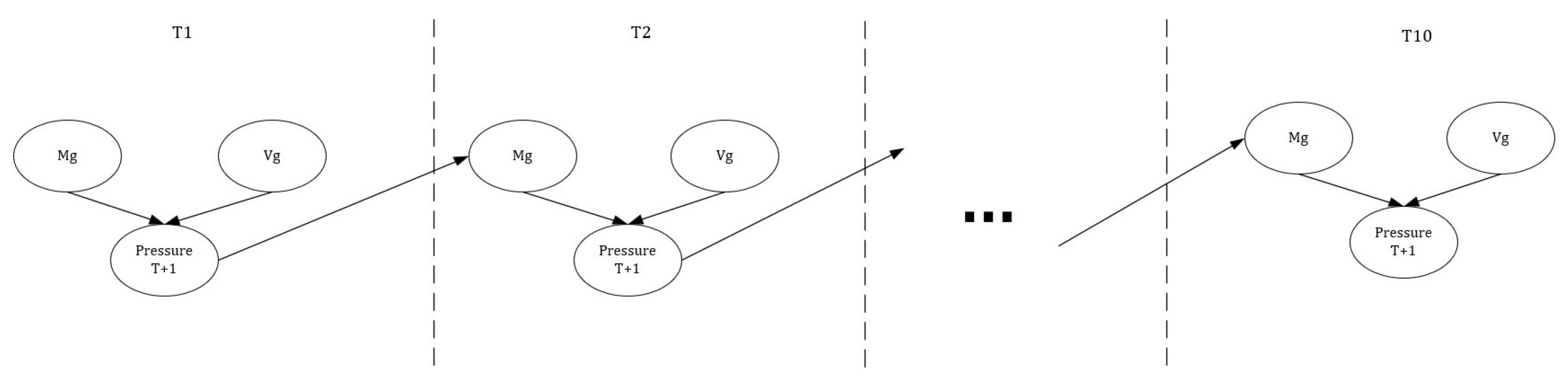
Figure 5.
Structure of a Dynamic Influence Diagram.
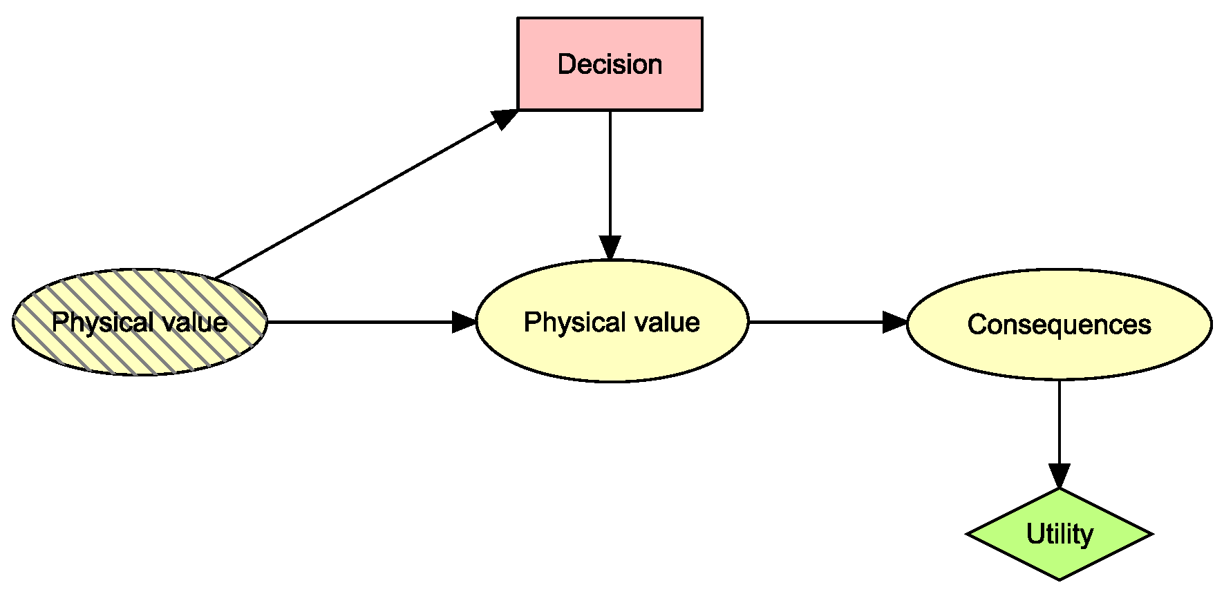
Figure 6.
Specialized Reinforcement Learning Agent (SRLA) framework.
Source: [17]
Figure 6.
Specialized Reinforcement Learning Agent (SRLA) framework.
Source: [17]
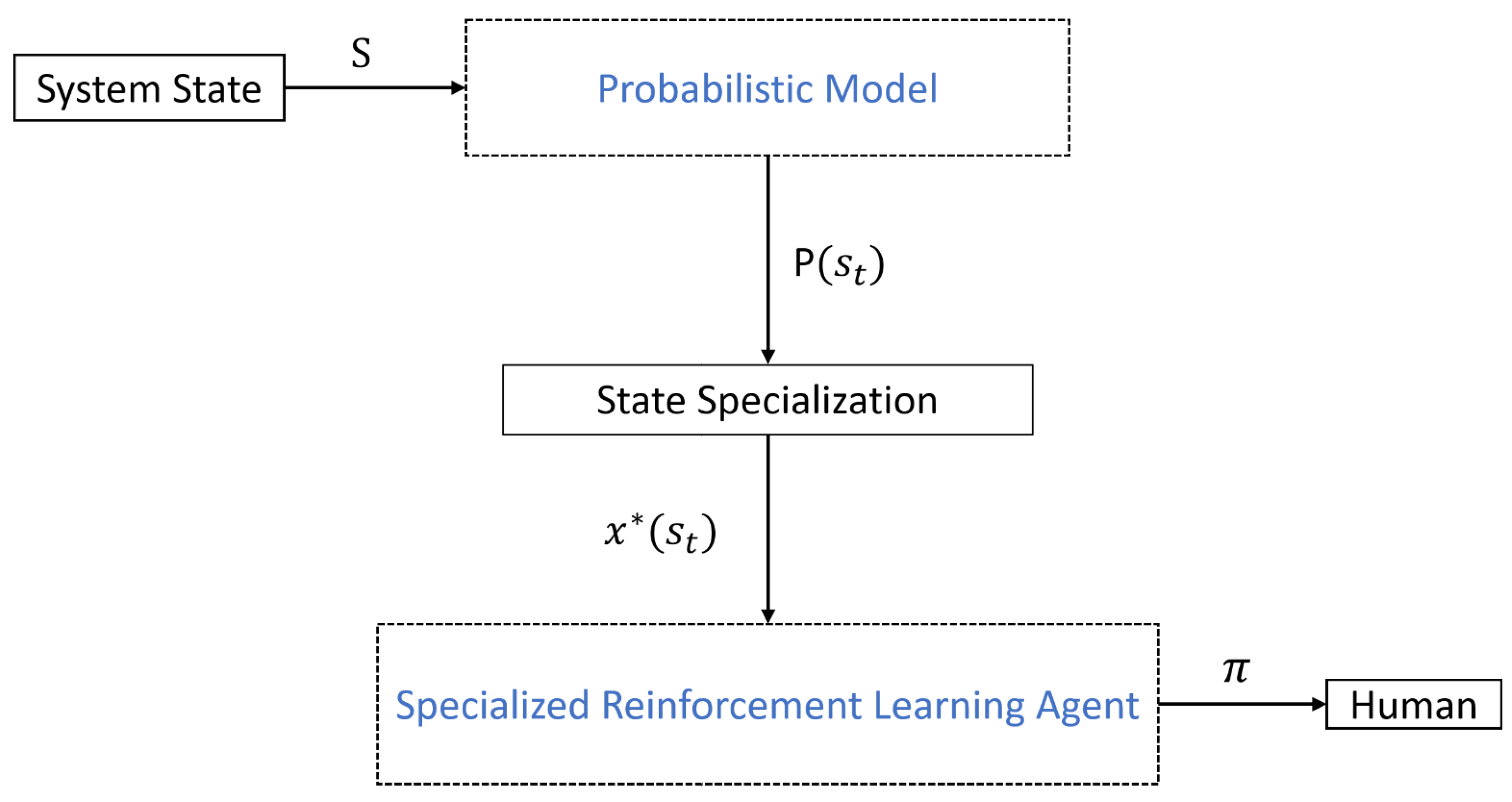
Figure 7.
Model designed for the 2 first scenarios. Pink nodes indicate decision variables: "Auto" (on/off states), "Set point" (representing nitrogen flow or pump power set points), and "System" (Primary/Secondary states reflecting the system in use for nitrogen flow). Yellow nodes represent random variables like physical values, faults, and consequences. Striped nodes indicate past variables affecting the current state. Green nodes are cost-associated with a specific state of the parent’s nodes.
Figure 7.
Model designed for the 2 first scenarios. Pink nodes indicate decision variables: "Auto" (on/off states), "Set point" (representing nitrogen flow or pump power set points), and "System" (Primary/Secondary states reflecting the system in use for nitrogen flow). Yellow nodes represent random variables like physical values, faults, and consequences. Striped nodes indicate past variables affecting the current state. Green nodes are cost-associated with a specific state of the parent’s nodes.
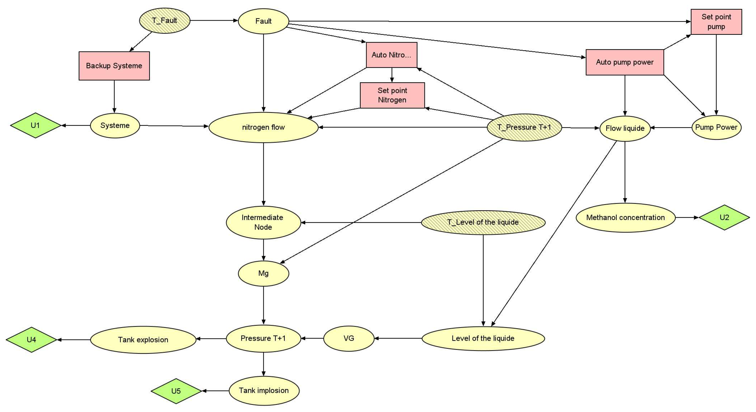
Figure 8.
Composite Model for Scenario Three: The upper module is responsible for adjusting the cooling water flow in the absorber’s, while the lower module advises on optimal cooling water temperature settings for the reactor.
Figure 8.
Composite Model for Scenario Three: The upper module is responsible for adjusting the cooling water flow in the absorber’s, while the lower module advises on optimal cooling water temperature settings for the reactor.
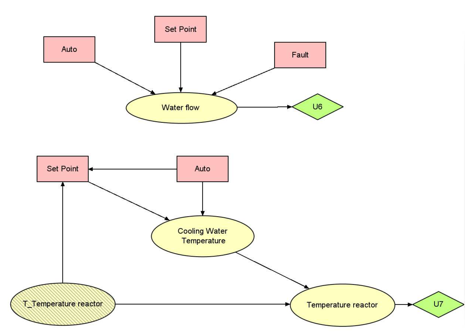
Figure 9.
Model used for anomaly detection for the two first scenarios.
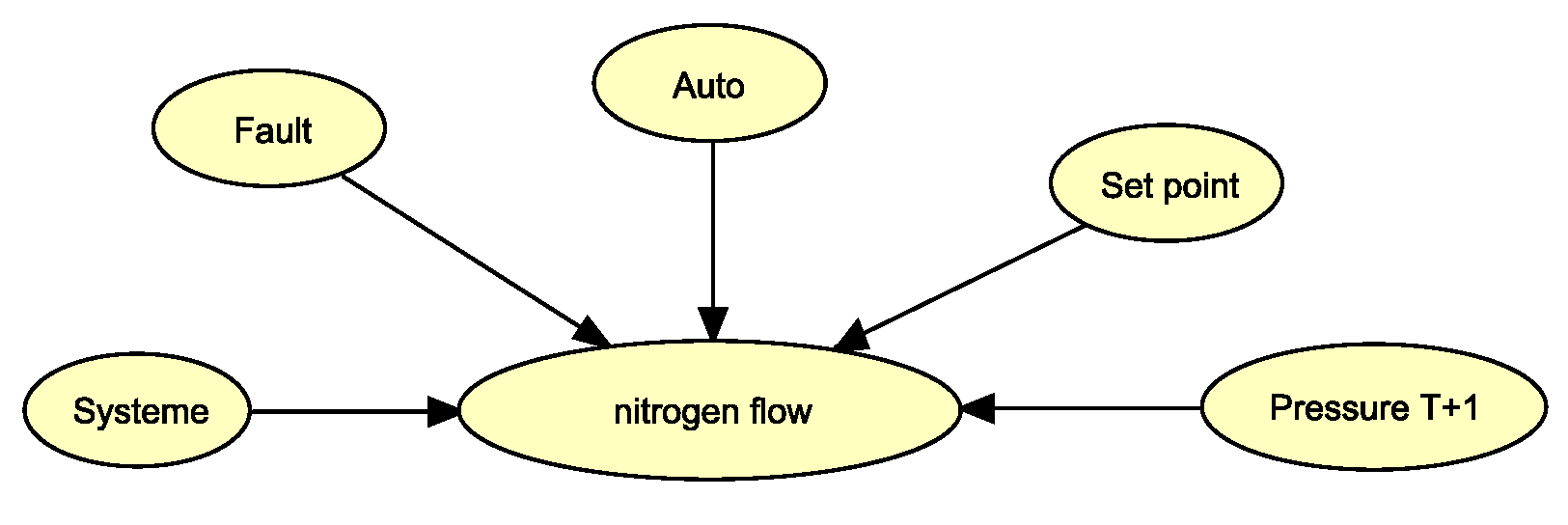
Figure 10.
Model used for anomaly detection for the third scenario.
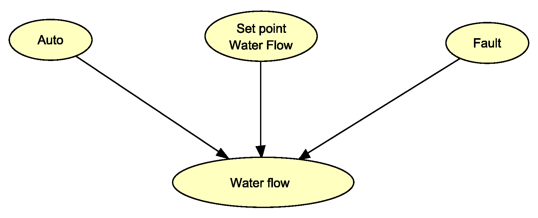
Figure 12.
Human-Centered Artificial Intelligence for Safety-Critical Systems (HAISC).
Source: [21].
Figure 12.
Human-Centered Artificial Intelligence for Safety-Critical Systems (HAISC).
Source: [21].
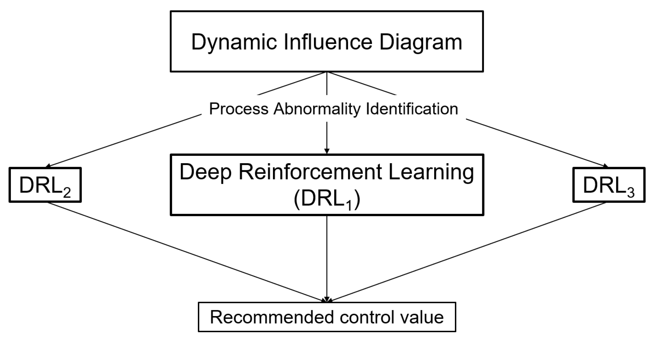
Figure 13.
Participant with the AI configuration (G2).
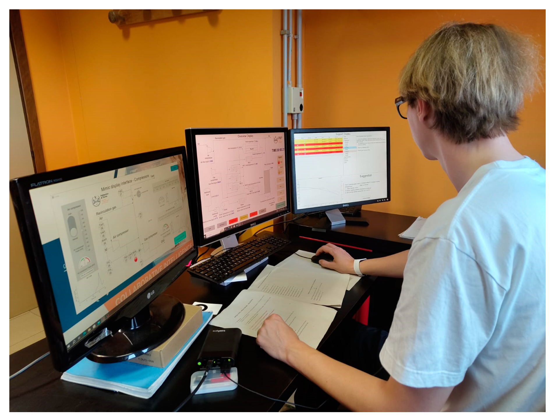
Figure 14.
Bar plot of the variable of the SART questionnaire for the two different groups. G1 without decision support and G2 with.
Figure 14.
Bar plot of the variable of the SART questionnaire for the two different groups. G1 without decision support and G2 with.
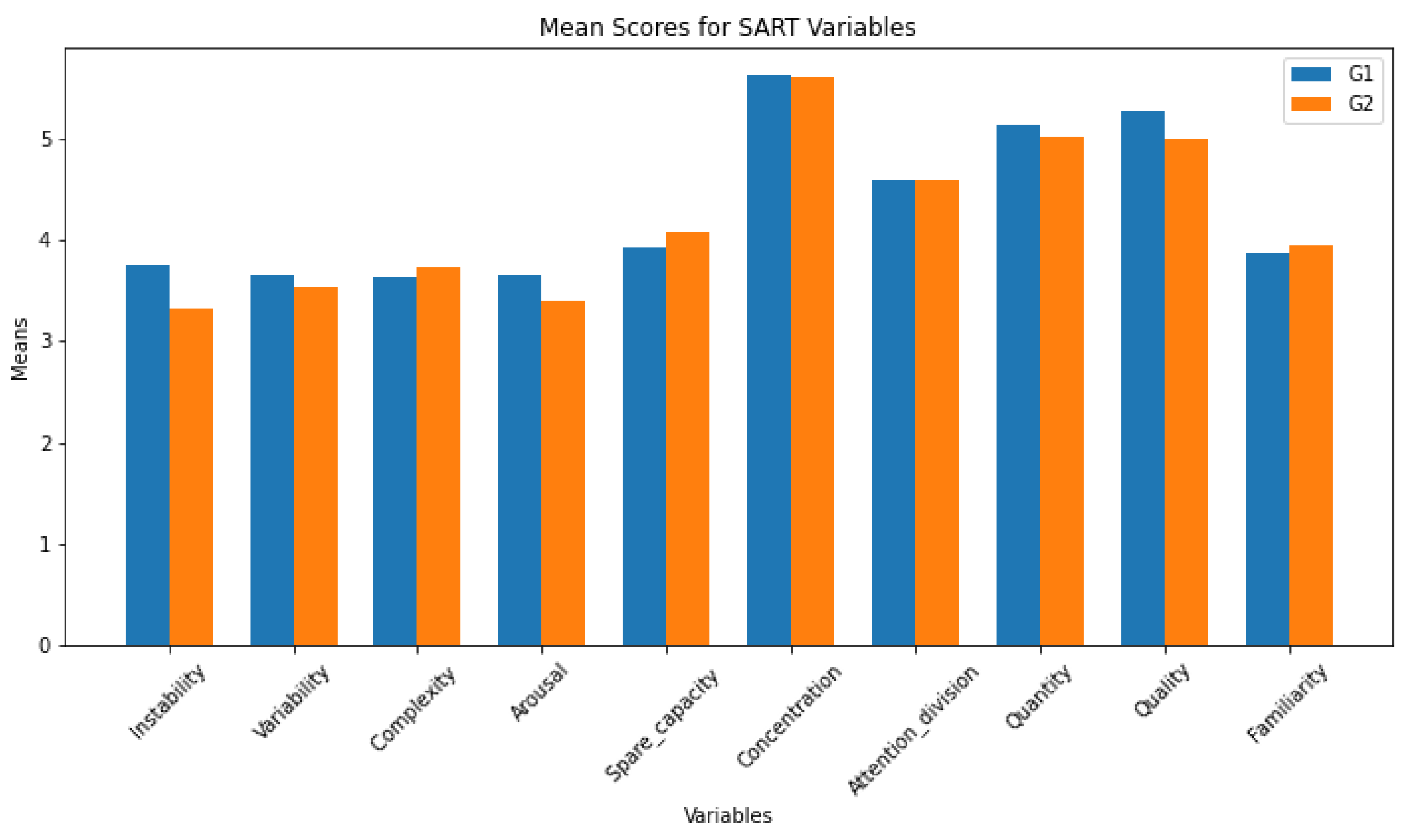
Figure 16.
Bar plot of the variable of the NASA TLX questionnaire for the two different groups. G1 without decision support and G2 with.
Figure 16.
Bar plot of the variable of the NASA TLX questionnaire for the two different groups. G1 without decision support and G2 with.
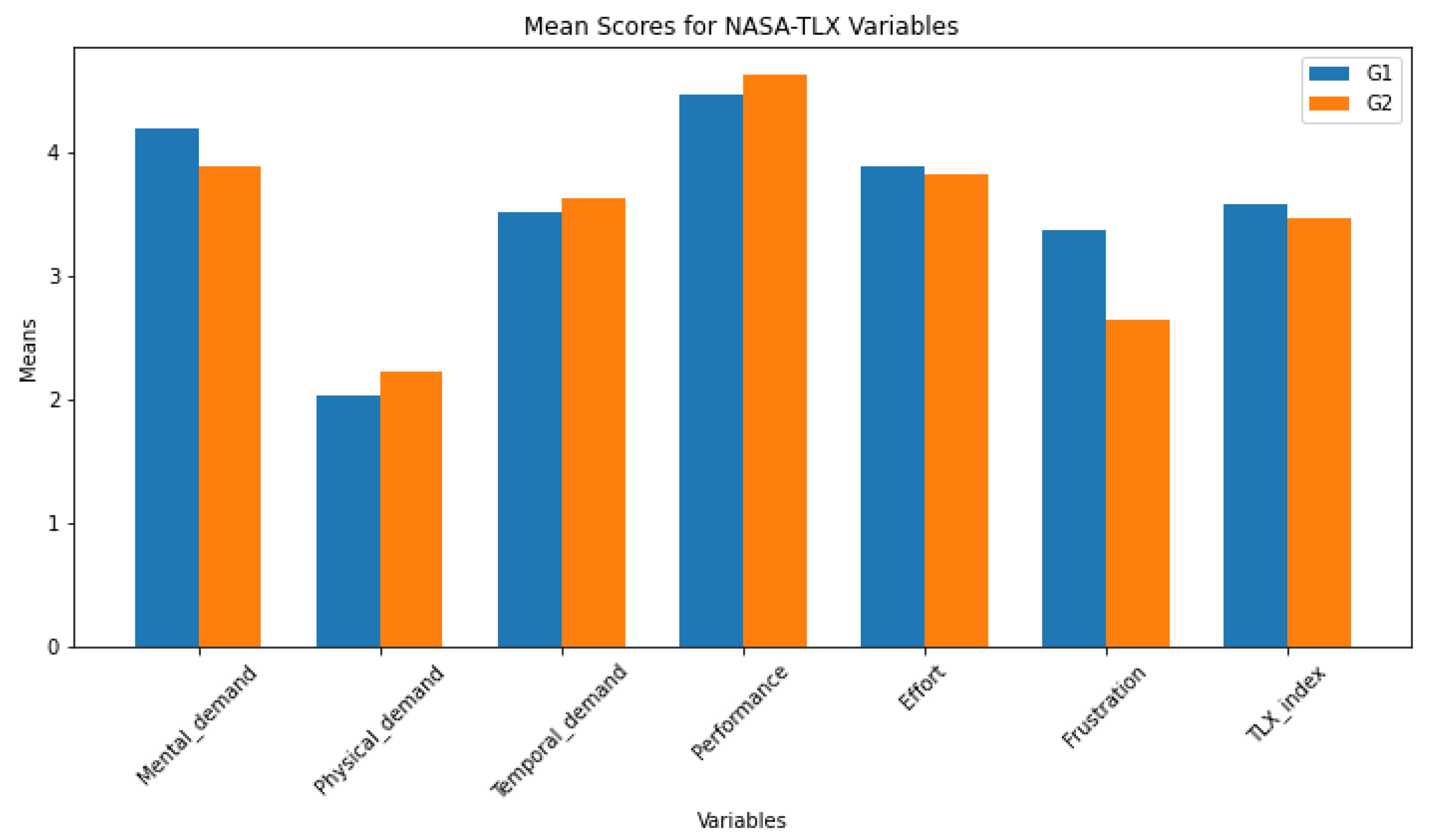
Figure 17.
Overall performance across all scenarios.
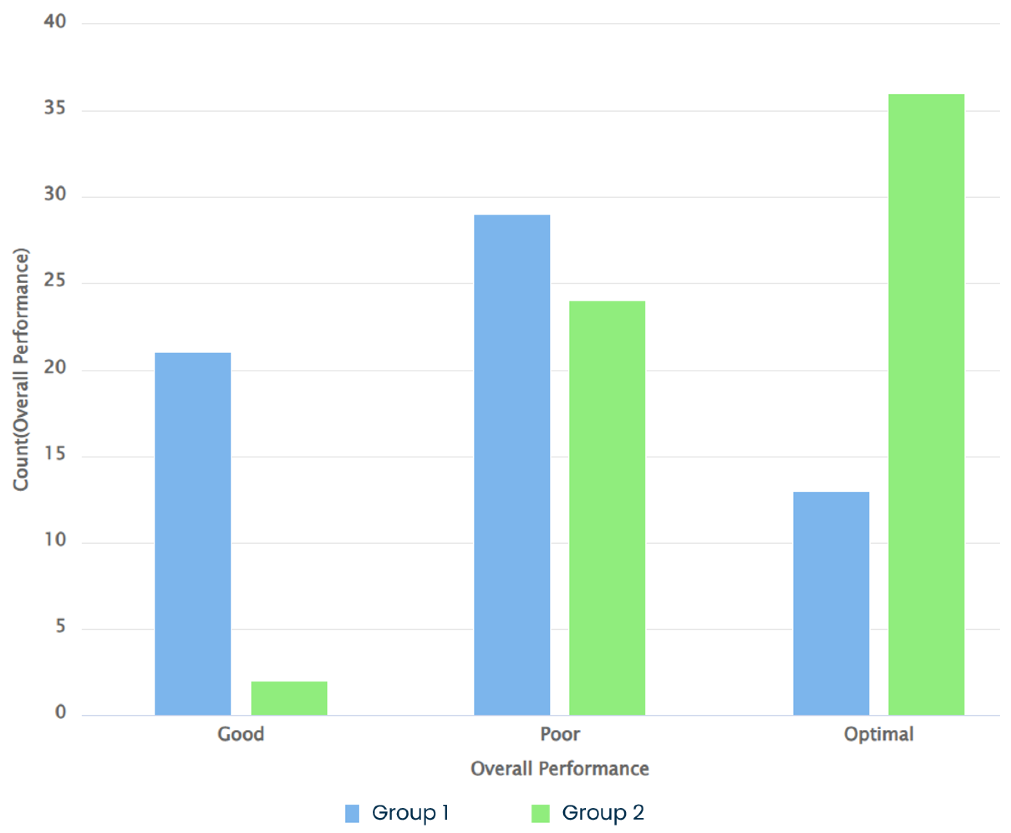

Table 1.
Statistical Test Results.
| Shapiro-Wilk G3 | Shapiro-Wilk G4 | Levene’s Test | t-test | Wilcoxon Rank-Sum Test | |
|---|---|---|---|---|---|
| Instability | 0.43 | 0.66 | 0.25 | 0.19 | 0.10 |
| Variability | 0.07 | 0.36 | 0.35 | 0.66 | 0.35 |
| Complexity | 0.22 | 0.39 | 0.63 | 0.75 | 0.42 |
| Arousal | 0.84 | 0.28 | 0.34 | 0.45 | 0.16 |
| Spare_capacity | 0.67 | 0.48 | 0.38 | 0.60 | 0.32 |
| Concentration | 0.016 | 0.18 | 0.58 | (0.97) | 0.33 |
| Attention_division | 0.05 | 0.96 | 0.88 | (0.99) | 0.39 |
| Quantity | 0.28 | 0.29 | 0.08 | 0.72 | 0.36 |
| Quality | 0.27 | 0.28 | 0.20 | 0.37 | 0.22 |
| Familiarity | 0.56 | 0.82 | 0.10 | 0.88 | 0.48 |
Table 2.
Statistical Test Results for SPAM Index and Related Factors.
| Shapiro-Wilk G1 | Shapiro-Wilk G2 | Levene’s Test | t-test | Wilcoxon Rank-Sum Test | |
|---|---|---|---|---|---|
| Monitoring | 0.00 | 0.10 | 0.01 | (0.00) | 0.00 |
| Planning | 0.38 | 0.36 | 0.13 | 0.14 | 0.09 |
| Intervention | 0.07 | 0.26 | 0.76 | (0.00) | 0.00 |
| SPAM_index | 0.16 | 0.61 | 0.03 | 0.00 | 0.00 |
Table 3.
Statistical Test Results.
| Shapiro-Wilk G3 | Shapiro-Wilk G4 | Levene’s Test | t-test | Wilcoxon Rank-Sum Test | |
|---|---|---|---|---|---|
| Mental_demand | 0.74 | 0.37 | 0.52 | 0.38 | 0.18 |
| Physical_demand | 0.04 | 0.00 | 0.20 | (0.56) | 0.47 |
| Temporal_demand | 0.81 | 0.05 | 0.28 | 0.72 | 0.37 |
| Performance | 0.53 | 0.01 | 0.05 | (0.61) | 0.16 |
| Effort | 0.54 | 0.72 | 0.68 | 0.85 | 0.41 |
| Frustration | 0.18 | 0.03 | 0.83 | (0.04) | 0.02 |
| TLX_index | 0.79 | 0.63 | 0.82 | 0.59 | 0.21 |
Table 4.
Time-based Performance Comparison per scenario.
| Reaction time | Response time | |||
|---|---|---|---|---|
| M | SD | M | SD | |
| S1 | ||||
| G1 | 276.30 | 46.35 | 339.30 | 150.39 |
| G2 | 106.96 | 130.96 | 259.04 | 170.13 |
| S2 | ||||
| G1 | 266.91 | 80.42 | 361.48 | 102.57 |
| G2 | 63.43 | 84.26 | 154.83 | 168.95 |
| S3 | ||||
| G1 | 190.17 | 117.22 | 787.87 | 207.56 |
| G2 | 117.38 | 55.78 | 680.00 | 226.43 |
Table 5.
Statistical test for significance between each group for each scenario.
| Wilcoxon Rank-Sum Test | |||
|---|---|---|---|
| S1 | S2 | S3 | |
| Reaction Time | 0.00 | 0.00 | 0.14 |
| Response Time | 0.07 | 0.00 | 0.08 |
| Overall Performance | 0.00 | 0.05 | 1.00 |
Table 6.
Temperature Data Comparison.
| Comparison | Shapiro-Wilk G1 | Shapiro-Wilk G2 | Levene’s Test | T-test | Wilcoxon Rank-Sum Test |
| Heart rate | 0.22 | 0.18 | 0.02 | 0.05 | 0.09 |
| Temperature | 0.46 | 0 | 0.98 | 0.13 | 0.1 |
| EDA | 0 | 0 | 0.19 | 0.17 | 0.21 |
Disclaimer/Publisher’s Note: The statements, opinions and data contained in all publications are solely those of the individual author(s) and contributor(s) and not of MDPI and/or the editor(s). MDPI and/or the editor(s) disclaim responsibility for any injury to people or property resulting from any ideas, methods, instructions or products referred to in the content. |
© 2023 by the authors. Licensee MDPI, Basel, Switzerland. This article is an open access article distributed under the terms and conditions of the Creative Commons Attribution (CC BY) license (http://creativecommons.org/licenses/by/4.0/).
Copyright: This open access article is published under a Creative Commons CC BY 4.0 license, which permit the free download, distribution, and reuse, provided that the author and preprint are cited in any reuse.


