Preprint
Article

Comparison of Pearson’s and Spearman’s Correlation Coefficients Values for Selected Traits of Pinus sylvestris L.

Altmetrics

Downloads

206

Views

176

Comments

0

Submitted:

20 December 2023

Posted:

21 December 2023

You are already at the latest version

Alerts
Abstract
The Spearman rank correlation coefficient is a non-parametric (distribution-free) rank statistic proposed by Charles Spearman as a measure of the strength of the relationship between two variables. It is a measure of a monotonic relationship that is used when the distribution of the data makes Pearson's correlation coefficient undesirable or misleading. The Spearman coefficient is not a measure of the linear relationship between two variables. It assesses how well an arbitrary monotonic function can describe the relationship between two variables, without making any assumptions about the frequency distribution of the variables. Unlike Pearson's product-moment (linear) correlation coefficient, it does not require the assumption that the relationship between variables is linear, nor does it require that the variables be measured on interval scales; it can be applied to variables measured at the ordinal level. The purpose of this study is to compare the values of Pearson's product-moment correlation coefficient (treating the data in a quantitative way) and Spearman's rank correlation coefficient (treating the same data in a somewhat "qualitative" way) and their statistical significance for six Pinus sylvestris L. traits (original – for Pearson's coefficient and ranked – for Spearman's coefficient) estimated from all observations, object means (for trees) and medians. The results show that the linear and rank correlation coefficients are consistent (as to direction and strength). In cases of divergence in the direction of correlation, the correlation coefficients were not statistically significant, which does not imply consistency in decision-making. Estimation of correlation coefficients based on medians is robust to outlier observations and factors that linear correlation is then very similar to rank correlation.
Keywords: 
Subject: Biology and Life Sciences  -   Forestry

1. Introduction

The study of trait interdependence (otherwise known as correlation) is a key area of data analysis in the life sciences, medicine, social sciences, economics and many other fields [1,2,3]. Correlation allows us to understand how different traits or variables interact with each other, which is important in the data analysis process [4]. Studying the correlation of traits makes it possible to identify patterns and relationships between different variables [5,6]. This allows the discovery of hidden relationships between data, which can lead to new research conclusions and hypotheses. Correlation enables the profiling of phenomena through the analysis of their interrelationships [7]. This facilitates a deeper understanding of the associations between various characteristics and helps identify factors that may influence the observed phenomena. The exploration of correlation enables the prediction of behaviors and trends by discerning patterns within historical data [8]. If two traits have a strong correlation, one can be used to predict the value of the other, which can be very important in stand research. Correlation analysis can help optimize production, marketing or resource management processes [9]. Studying correlations can lead to a better understanding of which factors affect efficiency and how performance can be improved [10,11].
In research, especially in statistics, correlation analysis helps select variables for further analysis. If two traits are highly correlated, it may suggest that both yield similar information, which may lead to the elimination of one of them to simplify the research model. While correlation does not imply causality, it can provide a starting point for further research into the causes of relationships between traits. Identifying a strong correlation can inspire researchers to dig deeper to understand why these traits are related [12,13,14].
In statistics, correlation is a measure of the strength and direction of a relationship between two variables. Correlation results are easy to understand and interpret. The correlation value ranges from -1 to 1, where 1 means perfect positive correlation, -1 means perfect negative correlation, and 0 means no correlation. This simple scale makes it easy to compare relationships between different variables and allows quick inferences about the strength of the relationship.
There are several different methods for calculating correlations, the two most popular being linear correlation (Pearson correlation) and rank correlation (Spearman correlation). Both types of correlation are used in scientific research, but differ in their assumptions and interpretation of results. Linear correlation measures the strength and direction of the relationship between two variables, assuming that the relationship between them is linear. Linear correlation assumes that changes in one variable are proportionally related to changes in the other variable. Linear correlation is sensitive to outliers, meaning that extreme values in the data can significantly affect the correlation result. Rank correlation is a non-linear measure of the relationship between two variables. Unlike linear correlation, it does not assume any restrictions on the shape of the relationship between variables. Instead, rank correlation is based on the order of the values in the two variables, transforming the observations into their respective ranks. Spearman correlation is then calculated based on the ranks of these observations. Rank correlation is less sensitive to outliers than linear correlation because it is based on the order of the ranks rather than the exact values of the data. Correlation analysis is very often performed on forest stand data [15,16,17,18,19].
The history and properties of the Pearson correlation coefficient have been described by Pearson [20], Weida [21], Walker [22], Stigler [23] and Piovani [24]. Pearson's correlation coefficient was discovered by Bravais in 1846 [25], but Karl Pearson was the first to describe a standard method of calculating it in 1896 [26] and showed that it was the best possible method. Pearson's important assumption is the normality of the analyzed variables, which can only be true for quantitative variables. Pearson's correlation coefficient is a measure of the strength of a linear relationship between two such variables. In 1904, Spearman [27] adopted the Pearson correlation coefficient as a measure of the strength of the relationship between two variables that cannot be measured quantitatively.
The purpose of this study was to analyze the correlation of six morphological traits of the needles of ten Scots pine (Pinus sylvestris L.) trees based on Pearson's linear correlation coefficients and Spearman's rank correlation. Correlation coefficients were estimated based on (1) all collected data from 30 needles for each tree, (2) mean values for individual trees and (3) medians for individual trees.

2. Materials and Methods

2.1. Study area

The analyses were carried out near the Belzec-Podlesin aeolian sand mine located near the town of Belzec (50°23′05″N, 23°24′04″E), in Eastern Roztocze [28], southeastern Poland, which operated in 2001-2008. The area was reclaimed after the closure of the open-pit mine. In 2019, one permanent experimental plot was established in the immediate vicinity of the sand mine by staff of the Department of Forest Engineering at the Poznań University of Life Sciences. The area of the experimental plot was 6.04 ha. Distance of the experimental plot centre from the topographical centre of the sand mine was 255.9726 m and the range of distances for individual trees was from 205.28 m to 293.24 m. Other characteristics of experimental plots: stand/share – pine/10, age/quality class – 74/I, forest habitat type – fresh coniferous forest, moisture content – fresh, and soil type – rusty podzolic soils.

2.2. Sampling

The field research was conducted in May 2019. The experimental plot was established at a distance of 255.9726 m from the topographic center of the sand mine. Then, ten randomly selected Scots pine trees growing in similar habitat conditions were cut in the plot and numbered from 1 to 10. Four shoots (three for analysis and one additional shoot) were taken from the top of each tree. The plant material was stored in a freezer at –18°C. A total of ten common pine needle samples were analyzed. For each of the ten common pine trees tested, 30 needles (one year old) were measured. A total of 300 randomly selected and correctly formed needles were measured.

2.3. Morphological and anatomical analysis

The needles were systematically examined between December 2020 and June 2021. These needles were extracted from branches that had been thawed to ambient temperature. Fresh needle samples were meticulously prepared from specimens stored in refrigeration, methodically extracted, and sectioned utilizing a manual cylindrical microtome (Euromex). Given the inherent variability in the structural composition of pine needles along their longitudinal axis [29], a consistent approach was employed: the needles were uniformly bisected longitudinally. Subsequent to this preparation, the specimens were meticulously preserved utilizing glycerin. Needle dimensions, specifically thickness and width, were measured under 10x magnification. Additionally, resin canals and stomatal apparatus were quantified on both the concave and convex surfaces of the needles. Following this preliminary analysis, each individually chosen needle underwent further scrutiny. Measurements were carried out employing a Dexter digital caliper and a Levenhuk 850B digital light microscope, featuring LevenhukLite software tailored to enhance the precision of these measurements. The length of each needle was measured with a precision of 0.01 cm. Subsequent analyses included determining epidermal and cuticular thickness, the thickness of individual hypodermal cells, and the diameter of individual resin canals. These parameters were scrutinized at a 40x magnification level, with measurements recorded to an accuracy of 0.01 µm. A total of six quantitative morphological and anatomical characteristics of needles were analyzed: needle length (NL), needle width (NW), needle thickness (NT), thickness of epidermis and cuticle (TEC), hypodermal cell thickness (HCT), resin duct diameter (RD). The method used to make the measurements is shown in Figure 1. The experience is described in detail in Wrońska-Pilarek et al. [30].

2.4. Statistical analysis

2.4.1. Pearson’s correlation

The Pearson’s correlation coefficient ( r P ) is a measure of the linear correlation between two sets of data: X and Y [31]:
r P = c o v X , Y σ X σ Y ,
where c o v X , Y – the covariance of two variables X and Y, σ X – the standard deviation of X, σ Y – the standard deviation of Y. The formula for c o v X , Y can be expressed in terms of mean and expectation:
c o v X , Y = E X μ X Y μ Y ,
where E(Z) – the expected value of a random variable Z, μ X – the mean of X, μ Y – the mean of Y. The formula for Pearson's correlation coefficient can be obtained by substituting estimates of the covariance and variance based on a sample into the formula (1). Given paired data x 1 , y 1 , , x n , y n   consisting of n pairs, r P is defined as:
r P = i = 1 n x i x ¯ y i y ¯ i = 1 n x i x ¯ 2 i = 1 n y i y ¯ 2
where n – sample size, x i and y i – the individual sample points indexed with i, x ¯ – the sample mean of X, y ¯ – the sample mean of Y.

2.4.2. Spearman’s correlation

Spearman's rank correlation coefficient ( r S ) is a nonparametric measure of rank correlation (statistical dependence between the rankings of two variables) [27]. The Spearman correlation coefficient is defined as the Pearson correlation coefficient between the rank variables. For a sample of size n, the n raw scores Xi, Yi are converted to ranks R(Xi), R(Yi), and r S is computed as:
r S = c o v R X , R Y σ R X σ R Y ,
where c o v R X , R Y – the covariance of the rank variables, σ R X – the standard deviation of the rank variable X, σ R Y – the standard deviation of the rank variable Y.

2.4.3. Data sets

Pearson's product-moment (linear) correlation coefficients and Spearman's rank correlation coefficients for the six Pinus sylvestris L. traits were calculated for three sets: (i) based on all observations, (ii) on object means (for trees), and (iii) on medians from empirical distributions.

2.4.4. Testing correlation coefficients

For pairs from an uncorrelated bivariate normal distribution, the sampling distribution of the studentized Pearson's correlation coefficient follows Student's t-distribution with n–2 degrees of freedom under the null hypothesis:
t = r n 2 1 r 2 ,
where r – linear Pearson’s correlation coefficient ( r P ) or Spearman's rank correlation coefficient ( r S ).
All analyses were performed using the GenStat v. 23 statistical software package [32].

3. Results

3.1. Correlation based on all observations

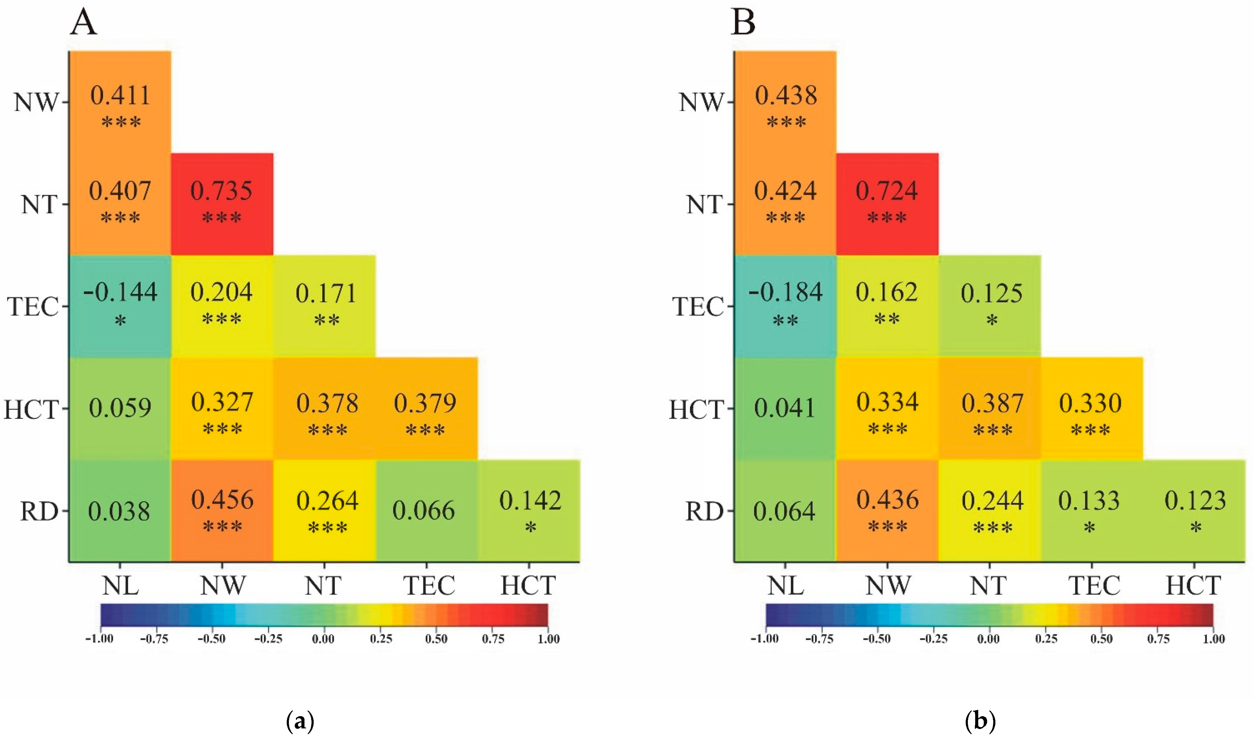
The direction of correlation, characterized by the sign of the correlation coefficient calculated from all observed data, was always consistent for linear correlation and rank correlation (Figure 2). The concordance of significance (or lack thereof) of linear correlation with rank correlation was almost perfect. Simultaneous significance of r P and r S correlation coefficients was not observed only between RD and TEC. For these two traits, a significant rank correlation was observed ( r S =0.133), with no linear correlation ( r P =0.066) (Figure 2).

3.2. Correlation calculated on object mean values

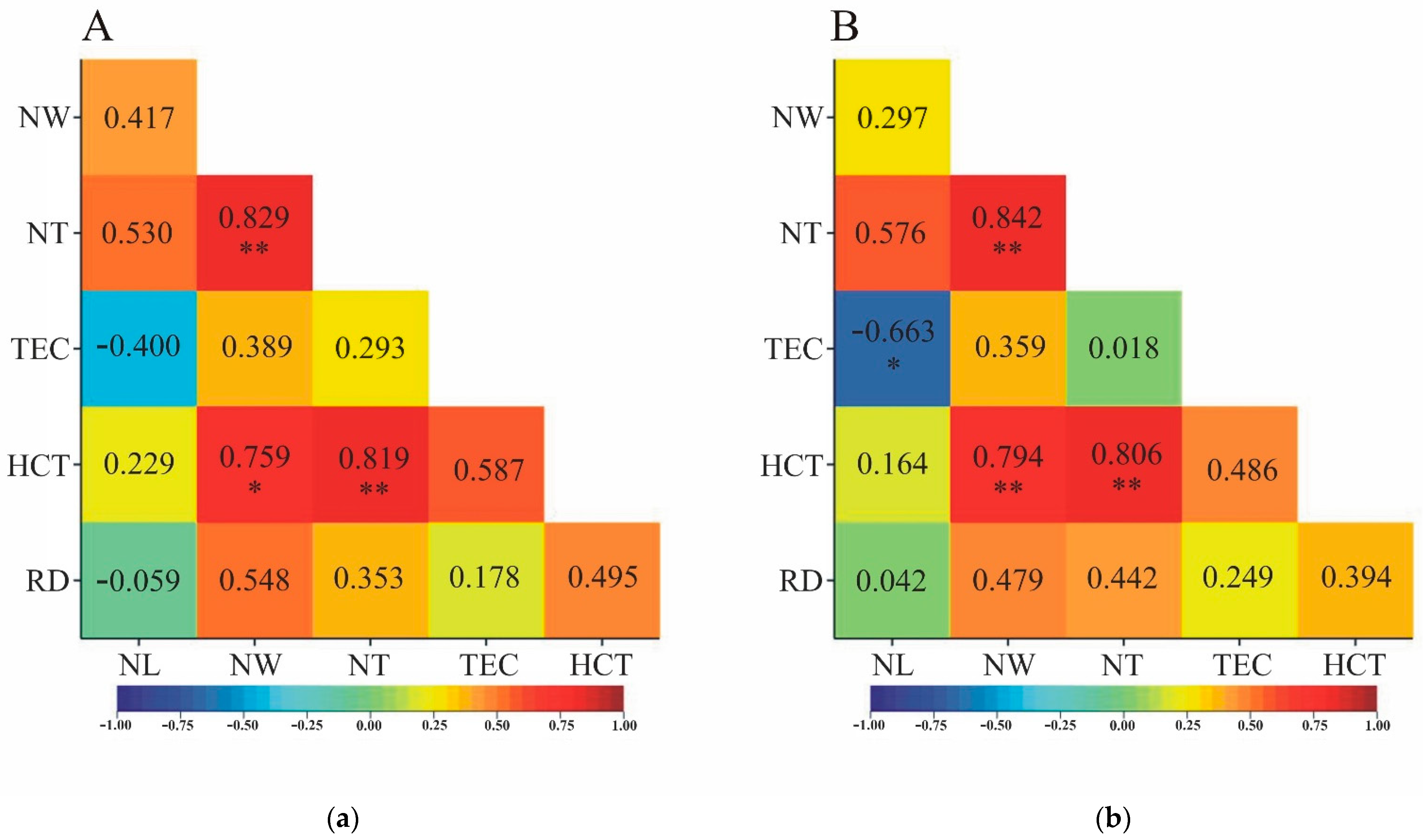
The signs of Pearson's and Spearman's correlation coefficients estimated from object averages were consistent for all pairs of traits except the RD-NL pair ( r P =-0.059, r S =0.042). However, both coefficients were not statistically significant (Figure 3). Analyzing the values of the correlation coefficients, concordance was observed in terms of their statistical significance for all pairs of traits except NL-TEC. Although both coefficients were negative, a statistically significant correlation coefficient between the two traits was observed only for ranks ( r S =-0.663) (Figure 3b).

3.3. Correlation calculated on medians from empirical distributions

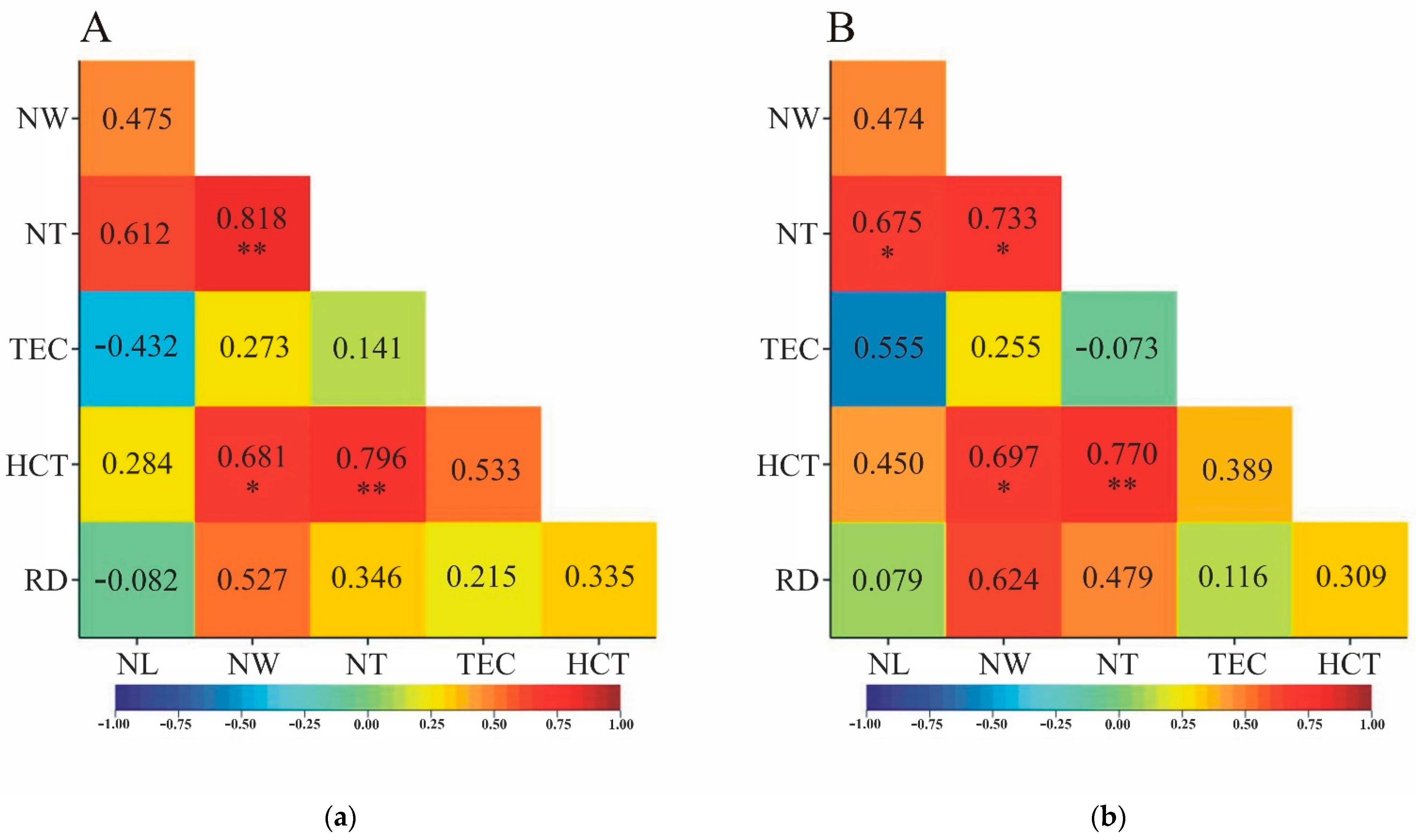
Correlation coefficients estimated from medians were characterized by sign agreement for linear and rank correlation except in two situations. For pairs of NL-TEC and NL-RD traits, linear correlation was inversely proportional – negative (-0.432 and -0.082, respectively), and rank correlation was positive (0.555 and 0.079, respectively). All four coefficients were not statistically significant (Figure 4). For most pairs of traits, the linear and rank correlation coefficients were statistically significant or insignificant at the same time (Figure 4a,b). Only between NL and NT was the opposite significance relationship observed: r P was not statistically significant (0.612; Figure 4a), and r S had a significance level of α=0.05 (0.675; Figure 4b).

3.4. Comparison between estimation methods

The most significant correlation coefficients were observed when correlation was estimated on the basis of all original observations – without recalculations (Figure 2). Significantly less significant correlation coefficients were found when they were estimated on the basis of object means or medians (Figure 3 and Figure 4). If a pair of traits was characterized by a significant correlation coefficient estimated from tree means or medians, it was also characterized by a significant correlation coefficient calculated on the basis of all observations. Pearson's linear correlation coefficients were equally significant (or simultaneously insignificant) when comparing estimation methods based on means and medians (Figure 3a and Figure 4a). For Spearman's rank correlation coefficients, such a relationship was not clear in two cases. NT correlated significantly with NL when the assessment of this relationship was done on medians, while it was not significant for the correlation coefficient estimated on tree means (Figure 3b and Figure 4b). In contrast, the opposite was true for the TEC-NL trait pair: the correlation coefficient based on mean values was statistically significant, while that based on medians was characterized by a lack of statistical significance (Figure 3b and Figure 4b).

4. Discussion

Correlation analysis is an extremely important tool in biology for understanding relationships between various biological variables [33,34,35,36]. Its importance includes identifying relationships between traits of organisms, studying the inheritance of genetic traits, analyzing the influence of environmental factors, and studying disease and health. This provides more precise information on the functioning of living organisms and the influence of external factors on their life and health [37,38,39].
Nevertheless, simply conducting a correlation analysis is only the beginning. By evaluating the results of such analysis, deeper insights into complex biological processes can be gained, which is crucial for further research, interpretation of results and decision-making in both science and practice [40].
Evaluation of correlation analysis helps identify potential errors and pitfalls in the data. Before evaluating correlation, make sure that the analyzed data is reliable and properly collected. Otherwise, the results of the analysis may be erroneous or misleading. When assessing the quality of the data, it is important to avoid false conclusions and ensure the reliability of the research.
Another key aspect of evaluating correlation analysis is to consider the biological context. Not all correlations are causal, meaning that even if there is a relationship between two variables, not necessarily one variable causes changes in the other. Correlation analysis should always be subjected to an evaluation of the biological context to avoid false interpretations. Otherwise, there is a risk of drawing incorrect conclusions about biological mechanisms [41,42].
Last but not least, the importance of assessing correlation analysis is to be able to predict the behavior of future variables based on known correlational relationships. In biology, especially in fields such as ecology or evolutionary biology, the ability to predict changes in populations or ecosystems is crucial for taking effective conservation measures or managing species populations [43,44,45].
In data analysis, especially in scientific research, the choice of appropriate statistical tools is crucial to obtaining reliable results. When the relationship between variables is studied, the question is often posed: is it worthwhile to simultaneously evaluate linear correlation and rank correlation? The answer to this question depends on the characteristics of the data and the purpose of the study [46]. In many cases, it is worth using both methods because they offer different perspectives on the relationship under analysis. Linear correlation is useful when the relationship between variables is linear. However, if the data contain outliers or do not meet the assumptions of normality, linear correlation can produce erroneous or misleading results. In such cases, rank correlation may be a more reliable alternative because it is less sensitive to outliers and does not require assumptions about the distribution of the data. In the research presented here, both measures were used to assess the correlation between the observed characteristics. Similarly, both measures, Pearson's and Sprearman's, were used in their studies, among others: Bonett and Wright [47], Artusi et al. [48], Hauke and Kossowski [49], and Eisinga et al. [50].
Assessing linear and rank correlation simultaneously provides a more complete picture of the relationship between variables. It may be that both methods indicate a similar relationship, which will strengthen our confidence in interpreting the results. In the study presented here, there was general agreement in the direction and significance of linear and rank correlation coefficients (Figure 2, Figure 3 and Figure 4). However, in the case of differing results, analysis of the two types of correlation can help identify specific traits of the data that affect the results of the analysis. Cases where the correlations did not agree were noted in the results obtained. In cases where the direction of correlation diverged, the correlation coefficients were not statistically significant, which does not imply consistency in decision-making. Linear and rank correlation coefficients with different signs were also obtained by other researchers: Udovičić et al. [51], Song and Park [52]. Simultaneous analysis of linear correlation and rank correlation can also help verify the results and ensure their reliability. If both methods indicate a similar relationship, our confidence in the veracity of the relationship increases. Such situations occurred in the results presented above on the correlation of six pine traits. If the results diverge, a closer examination of the data and potential reasons for the differences is necessary. A discrepancy in the context of significance/non-significance between Pearson's and Spearman's coefficients for a pair of TEC-RD traits requires a thorough investigation of the biological relationships between the traits.
The higher number of statistically significant correlation coefficients in the situation of evaluation on the basis of all original observations than for the converted data (to mean or median values) is due to the higher number of degrees of freedom in testing. For all observations, the number of degrees of freedom was 298, while for testing based on mean and median values it was 8. This resulted in smaller critical values when testing correlation coefficients based on all original observations.
Linear correlation is essential in regression analysis, which is a widely used technique in the social and natural sciences. Linear correlation makes it possible to assess the extent to which one variable can predict another. The results of linear correlation analysis are the basis for linear regression models, which make it possible to predict the value of one variable from another. This is especially important in studies of forest stands [53,54,55].
The estimation of rank correlation coefficients has its own unique advantages over the estimation of linear correlation coefficients. Its robustness to outliers, lack of requirements for data distribution, ability to detect nonlinear relationships, adaptability to different measurement scales, and greater flexibility in analyzing nonlinear data make it an attractive choice in many scientific fields. The estimation of rank correlation coefficients is particularly valuable for analyzing data that do not meet assumptions about the linear nature of relationships between variables, making it a versatile tool in scientific research [56,57].
Both correlation methods have their place in data analysis, and the choice between them depends on the nature of the variables and the assumptions of the study. If the relationship between the variables appears to be linear and there are no extreme outliers, linear correlation may be an appropriate tool. On the other hand, if a linear relationship cannot be assumed or there are outliers, rank correlation may provide more reliable results. With rank correlation, critical values are less prone to change at different levels of statistical significance, which can be useful in analyses where statistical significance is crucial. Since in the results of the presented study the number of observations for each tree was relatively large (30 observations), the choice of method for estimating correlation coefficients (based on means, medians or all data) does not seem to matter much. In the case of a large number of observations (n=300), two or three outlier observations will not disturb the significance of the actual correlations. Evaluation based on medians "compensates" for outlier observations to a large extent. In contrast, the median-based approach is completely immune to outlier observations, even when there are more of them. Rank correlation is less sensitive to differences in measurement scale between variables. This means that it can be used to analyze measurement data on both interval and ordinal scales, making it more flexible in application. It is important to always understand the characteristics of the data and use the appropriate correlation method to obtain reliable and interpretable results in scientific research.

5. Conclusions

Studying the interdependence of characteristics is crucial in data analysis, as it allows understanding the relationships between different variables. It makes it possible to discover new facts, make predictions, optimize processes and conduct effective scientific research. Correlation helps identify patterns and relationships, which is a fundamental step in the process of data analysis and scientific inference. Evaluation of the results of correlation analysis is as important as the analysis itself. Through careful evaluation, misinterpretations can be avoided, relationships between variables can be understood in the appropriate biological context, and changes in the systems under study can be predicted, all of which contribute to scientific progress and effective activities in the field of biology. Simultaneous evaluation of linear correlation and rank correlation is an effective strategy in analyzing relationships between variables. It makes it possible to get a comprehensive picture of the relationship between data, taking into account the diversity of data and differences in the characteristics of the variables under study. Using both methods, more certain and reliable results are obtained, which provide a solid basis for interpreting the relationships between the analyzed variables. The simultaneous use of linear correlation and rank correlation allows for a more complete understanding of the phenomena under study, which contributes to the progress of science and the formation of more precise theories and hypotheses. Estimation of correlation coefficients based on medians is robust to outlier observations and factors that linear correlation is then very similar to rank correlation.

Author Contributions

Conceptualization, J.B.; methodology, J.B., D.W.-P., A.K.-K., K.M. and B.W.; software, J.B.; validation, J.B., D.W.-P., A.K.-K., K.M. and B.W.; formal analysis, J.B.; investigation, J.B., D.W.-P., K.M. and B.W.; resources, A.K.-K.; data curation, A.K.-K., B.W. and K.M; writing—original draft preparation, J.B.; writing—review and editing, J.B., D.W.-P., A.K.-K., K.M. and B.W.; visualization, J.B. and A.K.-K.; supervision, J.B.; project administration, J.B.; funding acquisition, J.B. All authors have read and agreed to the published version of the manuscript.

Funding

This research received no external funding.

Data Availability Statement

The data in this manuscript are available from the corresponding author upon reasonable request.

Conflicts of Interest

The authors declare no conflict of interest.

References

  1. Fontana, M.D.; de Araújo Moreira, F.; Di Giulio, G.M.; Malheiros, T.F. The water-energy-food nexus research in the Brazilian context: What are we missing? Environ.Sci. Policy 2020, 112, 172–180. [CrossRef]
  2. Shimizu, I.; Kikukawa, M.; Tada, T.; Kimura, T.; Duvivier, R.; van der Vleuten, C. Measuring social interdependence in collaborative learning: instrument development and validation. BMC Med. Educ. 2020, 20, 177. [CrossRef]
  3. Tundys, B.; Bretyn, A.; Urbaniak, M. Energy Poverty and Sustainable Economic Development: An Exploration of Correlations and Interdependencies in European Countries. Energies 2021, 14(22), 7640. [CrossRef]
  4. Thielmann, I.; Spadaro, G.; Balliet, D. Personality and prosocial behavior: A theoretical framework and meta-analysis. Psychological Bulletin 2020, 146(1), 30–90. [CrossRef]
  5. Wright, I.J.; Ackerly, D.D.; Bongers, F.; Harms, K.E.; Ibarra-Manriquez, G.; Martinez-Ramos, M.; Mazer, S.J.; Muller-Landau, H.C.; Paz, H.; Pitman, N.C.A.; Poorter, L.; Silman, M.R.; Vriesendorp, C.F.; Webb, C.O.; Westoby, M.; Wright, S.J. Relationships Among Ecologically Important Dimensions of Plant Trait Variation in Seven Neotropical Forests. Ann. Bot. 2007, 99(5), 1003–1015. [CrossRef]
  6. Orsini, L.; Vanoverbeke, J.; Swillen, I.; Mergeay, J.; De Meester, L. Drivers of population genetic differentiation in the wild: isolation by dispersal limitation, isolation by adaptation and isolation by colonization. Mol. Ecol. 2013, 22, 5983–5999. [CrossRef]
  7. Alaimo, L.S.; Arcagni, A.; Fattore, M.; Maggino, F.; Quondamstefano, V. Measuring Equitable and Sustainable Well-Being in Italian Regions: The Non-aggregative Approach. Soc. Indic. Res. 2022, 161, 711–733. [CrossRef]
  8. Moews, B.; Herrmann, J.M.; Ibikunle, G. Lagged correlation-based deep learning for directional trend change prediction in financial time series. Expert Syst. Appl. 2019, 120, 197–206. [CrossRef]
  9. Min, Q.; Lu, Y.; Liu, Z.; Su, C.; Wang, B. Machine Learning based Digital Twin Framework for Production Optimization in Petrochemical Industry. Int. J. Inf. Manage. 2019, 49, 502–519. [CrossRef]
  10. Lin, W.B. Factors affecting the correlation between interactive mechanism of strategic alliance and technological knowledge transfer performance. J. High Technol. Manage. Res. 2007, 17(2), 139–155. [CrossRef]
  11. Lateef, M.; Keikhosrokiani, P. Predicting Critical Success Factors of Business Intelligence Implementation for Improving SMEs’ Performances: a Case Study of Lagos State, Nigeria. J. Knowl. Econ. 2023, 14, 2081–2106. [CrossRef]
  12. Dormann, C.F.; Elith, J.; Bacher, S.; Buchmann, C.; Carl, G.; Carré, G.; Marquéz, J.R.G.; Gruber, B.; Lafourcade, B.; Leitão, P.J.; Münkemüller, T.; McClean, C.; Osborne, P.E.; Reineking, B.; Schröder, B.; Skidmore, A.K.; Zurell, D.; Lautenbach, S. Collinearity: a review of methods to deal with it and a simulation study evaluating their performance. Ecography 2013, 36, 27–46. [CrossRef]
  13. Noor, M.B.T.; Zenia, N.Z.; Kaiser, M.S.; Al Mamun, S.; Mahmud, M. Application of deep learning in detecting neurological disorders from magnetic resonance images: a survey on the detection of Alzheimer’s disease, Parkinson’s disease and schizophrenia. Brain Inf. 2020, 7, 11. [CrossRef]
  14. Iqbal, W.; Tang, Y.M.; Chau, K.Y.; Irfan, M.; Mohsin, M. Nexus between air pollution and NCOV-2019 in China: Application of negative binomial regression analysis. Process Saf. Environ. Prot. 2021, 150, 557–565. [CrossRef]
  15. Ahmadi, K.; Kalantar, B.; Saeidi, V.; Harandi, E.K.G.; Janizadeh, S.; Ueda, N. Comparison of Machine Learning Methods for Mapping the Stand Characteristics of Temperate Forests Using Multi-Spectral Sentinel-2 Data. Remote Sens. 2020, 12(18), 3019. [CrossRef]
  16. Hyyppä, J,; Hyyppä, H.; Inkinen, M.; Engdahl, M.; Linko, S.; Zhu, Y.-H. Accuracy comparison of various remote sensing data sources in the retrieval of forest stand attributes. For. Ecol. Manage. 2000, 128(1–2), 109-120. [CrossRef]
  17. Puliti, S.; Breidenbach, J.; Astrup, R. Estimation of Forest Growing Stock Volume with UAV Laser Scanning Data: Can It Be Done without Field Data? Remote Sens. 2020, 12(8), 1245. [CrossRef]
  18. Moradi, F.; Darvishsefat, A.A.; Pourrahmati, M.R.; Deljouei, A.; Borz, S.A. Estimating Aboveground Biomass in Dense Hyrcanian Forests by the Use of Sentinel-2 Data. Forests 2022, 13(1), 104. [CrossRef]
  19. Wrońska–Pilarek, D.; Maciejewska–Rutkowska, I.; Lechowicz, K.; Bocianowski, J.; Hauke–Kowalska, M.; Baranowska, M.; Korzeniewicz, R. The effect of herbicides on morphological features of pollen grains in Prunus serotina Ehrh. in the context of elimination of this invasive species from European forests. Sci. Rep. 2023, 13, 4657. [CrossRef]
  20. Pearson, K. Notes on the history of correlation. Biometrika 1920, 13, 25–45.
  21. Weida, F.M. On various conceptions of correlation. Ann. Math. 1927, 29(1/4), 276–312.
  22. Walker, H.M. The relation of Plana and Bravais to theory of correlation. Isis 1928, 10(2), 466–484.
  23. Stigler, S.M. Francis Galton’s account of the invention of correlation. Stat. Sci. 1988, 4(2), 73–86.
  24. Piovani, J.I. The historical construction of correlation as a conceptual and operative instrument for empirical research. Qual. Quant. 2008, 42, 757–777.
  25. Bravais, A. Analyse mathématique sur les probabilités des erreurs de situation d’un point. Mémoires présentés par divers savants à l’Académie Royale des Sciences de l’Institut de France 1846, 9, 255–332.
  26. Pearson, K. Mathematical contributions to the theory of evolution. III. Regression, heredity, and panmixia. Phil. Trans. R. Soc. A 1896, 187, 253–318.
  27. Spearman, C. The Proof and Measurement of Association between Two Things. The Amer. J. Psychol. 1904, 15(1), 72–101. [CrossRef]
  28. Solon, J.; Borzyszkowski, J.; Bidłasik, M.; Richling, A.; Badora, K.; Balon, J.; Brzezińska-Wójcik, T.; Chabudziński, Ł.; Dobrowolski, R.; Grzegorczyk, I.; Jodłowski, M.; Kistowski, M.; Kot, R.; Krąż, P.; Lechnio, J.; Macias, A.; Majchrowska, A.; Malinowska, E.; Migoń, P.; Myga-Piątek, U.; Nita, J., Papińska, E.; Rodzik, J.; Strzyż, M.; Terpiłowski, S.; Ziaja, W. Physico-geographical mesoregions of Poland: Verification and adjustment of boundaries on the basis of contemporary spatial data. Geogr. Pol. 2018, 91(2), 143–170. [CrossRef]
  29. Jankowski, A.; Wyka, T.P.; Oleksyn, J. Axial variability of anatomical structure and the scaling relationships in Scots pine (Pinus sylvestris L.) needles of contrasting origins. Flora 2021, 274, 151747. [CrossRef]
  30. Wrońska-Pilarek, D.; Krysztofiak-Kaniewska, A.; Matusiak, K.; Bocianowski, J.; Wiatrowska, B.; Okoński, B. Does distance from a sand mine affect needle features in Pinus sylvestris L.? For. Ecol. Manage. 2023a, 546, 121276. [CrossRef]
  31. Pearson, K. On a mathematical theory of determinantal inheritance, from suggestions and notes of the late W. F. R. Weldon. Biometrika 1908, 6(1), 80–93. [CrossRef]
  32. VSN International Genstat for Windows, 23rd Edition; VSN International: Hemel Hempstead, UK, 2023.
  33. Carter, B.E.; Wiles, J.R. Scientific consensus and social controversy: exploring relationships between students’ conceptions of the nature of science, biological evolution, and global climate change. Evo. Edu. Outreach 2014, 7, 6. [CrossRef]
  34. Rosato, A.; Tenori, L.; Cascante, M.; De Atauri Carulla, P.R.; dos Santos, V.A.P.M.; Saccenti, E. From correlation to causation: analysis of metabolomics data using systems biology approaches. Metabolomics 2018, 14, 37. [CrossRef]
  35. Rutledge, J.; Oh, H.; Wyss-Coray, T. Measuring biological age using omics data. Nat. Rev. Genet. 2022, 23, 715–727. [CrossRef]
  36. Saalidong, B.M.; Aram, S.A.; Otu, S.; Lartey, P.O. Examining the dynamics of the relationship between water pH and other water quality parameters in ground and surface water systems. PLoS ONE 2022, 17(1), e0262117. [CrossRef]
  37. Tortella, G.R.; Rubilar, O.; Durán, N.; Diez, M.C.; Martínez, M.; Parada, J.; Seabra, A.B. Silver nanoparticles: Toxicity in model organisms as an overview of its hazard for human health and the environment. J. Hazard. Mater. 2020, 390, 121974. [CrossRef]
  38. Waszak, N.; Robertson, I.; Puchałka, R.; Przybylak, R.; Pospieszyńska, A.; Koprowski, M. Investigating the Climate-Growth Response of Scots Pine (Pinus sylvestris L.) in Northern Poland. Atmosphere 2021, 12(12), 1690. [CrossRef]
  39. Samal, K.; Mahapatra, S.; Ali, H. Pharmaceutical wastewater as Emerging Contaminants (EC): Treatment technologies, impact on environment and human health. Energy Nexus 2022, 6, 100076. [CrossRef]
  40. Nowosad, K.; Bocianowski, J.; Kianersi, F.; Pour-Aboughadareh, A. Analysis of Linkage on Interaction of Main Aspects (Genotype by Environment Interaction, Stability and Genetic Parameters) of 1000 Kernels in Maize (Zea mays L.). Agriculture 2023, 13(10), 2005. [CrossRef]
  41. Broadhurst, D.I.; Kell, D.B. Statistical strategies for avoiding false discoveries in metabolomics and related experiments. Metabolomics 2006, 2, 171–196. [CrossRef]
  42. Nakagawa, S.; Cuthill, I.C. Effect size, confidence interval and statistical significance: a practical guide for biologists. Biol. Rev. 2007, 82, 591–605. [CrossRef]
  43. Clutton-Brock, T.; Sheldon, B.C. Individuals and populations: the role of long-term, individual-based studies of animals in ecology and evolutionary biology. Trends Ecol. Evol. 2010, 25(10), 562–573. [CrossRef]
  44. Dwyer, R.G.; Krueck, N.C; Udyawer, V.; Heupel, M.R.; Chapman, D.; Pratt, Jr., H.L.; Garla, R.; Simpfendorfer, C.A. Individual and Population Benefitsof Marine Reserves for Reef Sharks. Curr. Biol. 2020, 30, 480–489. [CrossRef]
  45. Hohenlohe, P.A.; Funk, W.C.; Rajora, O.P. Population genomics for wildlife conservation and management. Mol. Ecol. 2021, 30, 62–82. [CrossRef]
  46. Horváth, I.G.; Németh, Á.; Lenkey, Z.; Alessandri, N.; Tufano, F.; Kis, P.; Gaszner, B.; Cziráki, A. Invasive validation of a new oscillometric device (Arteriograph) for measuring augmentation index, central blood pressure and aortic pulse wave velocity. J. Hypertens. 2010, 28(10), 2068–2075. [CrossRef]
  47. Bonett, D.G., Wright, T.A. Sample size requirements for estimating Pearson, Kendall and Spearman correlations. Psychometrika 2000, 65, 23–28. [CrossRef]
  48. Artusi, R.; Verderio, P.; Marubini, E. Bravais-Pearson and Spearman Correlation Coefficients: Meaning, Test of Hypothesis and Confidence Interval. Int. J. Biol. Markers 2002, 17(2), 148–151. [CrossRef]
  49. Hauke, J.; Kossowski, T. Comparison of values of Pearson’s and Spearman’s correlation coefficient on the same sets of data. Quaestiones Geographicae 2011, 30(2), 87–93. [CrossRef]
  50. Eisinga, R.; Grotenhuis, M.t.; Pelzer, B. The reliability of a two-item scale: Pearson, Cronbach, or Spearman-Brown?. Int. J. Public Health 2013, 58, 637–642. [CrossRef]
  51. Udovičić, M.; Baždarić, K.; Bilić-Zulle, L.; Petrovečki, M. What we need to know when calculating the coefficient of correlation? Biochemia Medica 2007, 17(1), 10–15.
  52. Song, H.Y.; Park, S. An Analysis of Correlation between Personality and Visiting Place using Spearman’s Rank Correlation Coefficient. KSII Trans. Internet Inf. Syst. 2020, 14(5), 1951–1966. [CrossRef]
  53. Neumann, M.; Starlinger, F. The significance of different indices for stand structure and diversity in forests. For. Ecol. Manage. 2001, 145(1–2), 91–106. [CrossRef]
  54. Lefsky, M.A.; Hudak, A.T.; Cohen, W.B.; Acker, S.A. Patterns of covariance between forest stand and canopy structure in the Pacific Northwest. Remote Sens. Environ. 2005, 95(4), 517–531. [CrossRef]
  55. Ali, A. Forest stand structure and functioning: Current knowledge and future challenges. Ecol. Indic. 2019, 98, 665–677. [CrossRef]
  56. Schober, P.; Boer, C.; Schwarte, L.A. Correlation Coefficients: Appropriate Use and Interpretation. Anesthesia & Analgesia 2018, 126(5), 1763–1768. [CrossRef]
  57. Lindinger-Sternart, S.; Kaur, V.; Widyaningsih, Y.; Patel, A.K. COVID-19 phobia across the world: Impact of resilience on COVID-19 phobia in different nations. Couns Psychother Res. 2021, 21, 290–302. [CrossRef]
Figure 1. The method used to measure analyzed needle traits: NL – needle length, NW – needle width, NT – needle thickness, TEC – thickness of epidermis and cuticle, HCT – hypodermal cell thickness, RD – resin duct diameter.
Preprints 93932 g001
Figure 2. Comparison of Pearson's (a) and Spearman's (b) correlation coefficients of selected Pinus sylvestris L. traits calculated from all observations. NL – needle length, NW – needle width, NT – needle thickness, TEC – thickness of epidermis and cuticle, HCT – hypodermal cell thickness, RD – resin duct diameter. * – p<0.05; ** – p<0.01; *** – p<0.001; n=300.
Preprints 93932 g002
Figure 3. Comparison of Pearson's (a) and Spearman's (b) correlation coefficients of selected Pinus sylvestris L. traits calculated from tree averages. NL – needle length, NW – needle width, NT – needle thickness, TEC – thickness of epidermis and cuticle, HCT – hypodermal cell thickness, RD – resin duct diameter. * – p<0.05; ** – p<0.01; n=10.
Preprints 93932 g003
Figure 4. Comparison of Pearson's (a) and Spearman's (b) correlation coefficients of selected Pinus sylvestris L. traits calculated from median. NL – needle length, NW – needle width, NT – needle thickness, TEC – thickness of epidermis and cuticle, HCT – hypodermal cell thickness, RD – resin duct diameter. * – p<0.05; ** – p<0.01; n=10.
Preprints 93932 g004
Disclaimer/Publisher’s Note: The statements, opinions and data contained in all publications are solely those of the individual author(s) and contributor(s) and not of MDPI and/or the editor(s). MDPI and/or the editor(s) disclaim responsibility for any injury to people or property resulting from any ideas, methods, instructions or products referred to in the content.
Copyright: This open access article is published under a Creative Commons CC BY 4.0 license, which permit the free download, distribution, and reuse, provided that the author and preprint are cited in any reuse.
Prerpints.org logo

Preprints.org is a free preprint server supported by MDPI in Basel, Switzerland.

Subscribe

© 2024 MDPI (Basel, Switzerland) unless otherwise stated