
Submitted:
11 December 2023
Posted:
12 December 2023
You are already at the latest version
Abstract
In this paper, we present a new parametric class of optimal fourth-order iterative methods to estimate the solutions of nonlinear equations. After the convergence analysis, we study the stability of this class by using the tools of complex discrete dynamics. This allows us to select those elements of the class with lower dependence on initial estimations. We verify by means of numerical tests that the stable members on quadratic polynomials perform better than the unstable ones, when applied to other non-polynomial functions. We also compare the performance of the best elements of the family with known methods, such as the schemes by Newton or Chun, among others, showing robust and stable behaviour.
Keywords:
Iterative methods
; convergence order
; periodic orbits
; stability
; analytical conjugation
; parameter plane
; dynamical plane.
1. Introduction and Preliminary Concepts
Numerical methods play a fundamental role in scientific and engineering disciplines due to their ability to solve mathematical equations, enabling the analysis of physical phenomena and complex systems. These algorithms provide approximate solutions when exact solutions are challenging to obtain, while also offering computational efficiency in terms of time and computational resources by effectively performing complex calculations.
In the field of numerical analysis, there is a current trend of designing families of numerical methods that generalize existing approaches. Notable examples include King’s family [23] and that developed by Hueso et al. in [20]. Some of these methods incorporate weight functions in their design process (see, for example, [11,12,14]).
The efficiency index of an iterative method is defined by Ostrowski in [26] as , where p is the order of convergence and d is the number of functional evaluations per iteration. This concept is directly related with Kung-Traub’s Conjecture [24], that states the order of convergence of any iterative scheme cannot be greater than (called optimal order).
Several authors have generalized iterative schemes optimally according to Kung-Traub’s conjecture [24]. However, since there is no difference in the number of function evaluations and the order of the members within a family of iterative methods, it is necessary to conduct a stability study on some simple nonlinear functions, such as quadratic polynomials. This is because in practice, it has been observed that iterative schemes that are stable for such functions tend to perform better compared to other methods that exhibit some pathology when applied to more complicated functions. To this end, complex discrete dynamics are employed to analyze stability in functions like quadratic polynomials (see, for example, the work of Amat et al. in [1,2], Behl et al. in [3], Chicharro et al. in [9], Cordero et al. in [15,16,17]), Khirallah et al. [22], Moccari et al. in [25], among others.
The detailed description of the following concepts in complex dynamics can be found in [4,19]. Let be a rational function on the Riemann sphere , then we denote by the operator , where and are complex polynomials with no common factors. Usually, R is obtained by applying an iterative scheme on a quadratic polynomial .
Given , we define the orbit of under R to be the sequence of points . Point is called the seed of the orbit. There are many different kind of orbits in a typical dynamical system. Undoubtedly, the most important kind of orbit is a fixed point, that is, a point that satisfies . Another important element is the periodic orbit or cycle. A point is n-periodic if for some , being for any . The least such n is called the prime period of the orbit.
Let us suppose that is a fixed point of R. Then is an attracting fixed point if . The point is a repelling fixed point if and, finally, if , the fixed point is called neutral or indifferent.
Theorem 1.
[19] Attracting Fixed Point Theorem. Suppose is an attracting fixed point for R. Then there exists a domain D contained within the Riemann sphere such that and in which the following condition is satisfied: if , then for all n and, moreover, as .
Theorem 2.
[19] Repelling Fixed Point Theorem. Suppose is a repelling fixed point for R. Then there exists a domain D contained within the Riemann sphere such that and in which the following condition is satisfied: if and , then there is an integer such that .
Now, let us suppose is an attracting fixed point for R. The basin of attraction of is the set of all points whose orbits tend to . The immediate basin of attraction of is the largest convex component containing that lies in the basin of attraction. The critical points of the operator are those that meet . A critical point is called free if it does not match with the roots of the polynomial. These two concepts are closely related with the next result.
Theorem 3.
Fatou and Julia studied the iteration of rational maps under the assumption that . They focused on a disjoint invariant decomposition of into two sets. One of these sets is often called the Julia set. The other set we shall refer to it as the Fatou set [4]. The Fatou set is the union of all basins of attraction, and the Julia set is its boundary.
By Theorem 3, all the attracting behaviour of a rational function can be found by iterating the free critical points and classifying them by their asymptotical performance in the Fatou set. This is done by means of the parameter plane, in case the rational function R depends on a complex parameter . It is the graphical representation that provides information about the choice of one or another value of a parameter within a family of iterative methods. This graphical representation directly relates each point in the complex plane to its corresponding parameter value that specifies each member of the family. Given a free critical point of R used as initial estimation, the parameter plane indicates which attracting periodic orbit or fixed point the orbit of the critical point converges to.
When all the free critical points are known, we calculate the parameter planes to determine which values of relates the final state of all free critical points to any of the roots of . According to Theorem 3, this will ensure stability (on quadratic polynomials) of the associated elements of the class, as the only basins of attraction correspond with these roots.
Given a free critical point as a seed of the rational function R, we define as the set of values of where the free critical point is in the basin of attraction of any of the roots of .
We also define the characteristic function of the set as:
Therefore, we consider the parameter plane by representing the characteristic function of , where the red color is assigned when and black when .
Our interest is to determine the values of in which the final state of the orbits of all free critical points is one of the polynomial roots. Since we construct a parameter plane for each free critical point, we proceed to construct the intersection of the parameter planes, that is called unified parameter plane [10]. In this plane, we graph , where n is the number of free critical points of the rational operator. Each red-colored point corresponds to values of for which all members of the family of iterative schemes are stable on quadratic polynomials.
One way to validate the information obtained through parameter planes is by using dynamical planes, which graphically represent the basins of attraction of a set of initial values for a specific member of the family, that is, for a value of . In other words, given a parameter value for which the associated method is stable, its dynamical plane is composed only of the basins of the polynomial roots. This indicates that, regardless of the initial estimate of the method, it will always be able to converge to one of the roots. On the other hand, if the parameter value is in the instability region on the parameter plane, in addition to the basins of the roots, other basins corresponding to attracting periodic or strange fixed points appear. Through the dynamical planes, we determine to which attracting fixed point the orbit of any initial estimate converges for a specific value of .
The basin of attraction for the root is represented in orange color, while the basin for is represented in blue. Additionally, we assign different colors such as green, red, etc., depending on the number of attracting fixed points associated with , and we use black to represent basins of periodic orbits. The decrease in brightness of each color is an indicator of the size of the orbit of each point, meaning that brighter colors represent points that require fewer iterations to reach the fixed or periodic point. The codes used to present the parameter and dynamical planes are defined by Chicharro et al. in [8].
Let us remark that all the information obtained depends on the quadratic polynomial used to define the rational function R, by applying the class of iterative methods on it. A key tool to extend these results to any quadratic polynomial is the conjugation. Let f and g be two functions from the Riemann sphere to itself. An analytic conjugation between f and g is a diffeomorphism h of the Riemann sphere onto itself such that , where h is called the conjugation. In [5], Blanchard introduced the conjugation map , which is a Möbius transformation satisfying the following properties: , , and being a and b the roots of the arbitrary quadratic polynomial .
Theorem 4.
If a family of iterative methods satisfies the Scaling Theorem, then the Möbius transformation can be applied. As demonstrated by Blanchard in [4], the asymptotic behavior of the system is qualitatively equivalent under conjugation. This allows us to perform dynamical analysis on an associated operator that does not depend on the roots a and b. Instead, the dynamical study is conducted based on their corresponding values in the new operator, which are and . Additionally, the strange fixed point corresponds to the divergence of the original method. This makes the analysis of its stability particularly important.
In this investigation, using the weight function technique in Section 2, a parametric family of iterative methods of order four is designed. In Section 3, the rational function resulting from the fixed point operator applied on a quadratic polynomial is analyzed. More specifically, we study the dynamics of the fixed points of this rational operator R, which allows us to determine its stability. Also, in Section 4, the numerical behavior of some of the most stable members on other non-polynomial functions is analyzed and compared with other known methods in the literature. Finally, in Section 5, some conclusions are presented, highlighting the most significant findings of the research.
2. Construction of a New Parametric Family of Iterative Methods
If is a nonlinear equation, then an iterative method, under certain conditions, generates a sequence of real numbers that converges to a solution . However, the guarantee of convergence to a solution, the convergence rate, and the solution to which an iterative scheme converges all have a direct dependence on the initial estimate. The creation of a new class of iterative methods makes sense as long as there are members of the family that are competitive compared to existing schemes with good behavior. In our study, we present a new family of iterative methods using the weight function procedure, characterized by:
where is an arbitrary parameter and H is a real function depending on . Now, we present the convergence result of this family, describing the conditions that function must satisfy in order to achieve fourth-order convergence of (1).
Theorem 5.
Let a simple zero of a sufficiently differentiable function and . Let us assume an initial estimation close enough to a zero of f. If a weight function , , is chosen satisfying , , and , then class (1) has fourth-order of convergence if and only if , being the error equation is given by
where and
Proof.
By applying the Taylor expansion of on , we have:
and
dividing directly (2) by (3) we get
If in the first step of (1) we subtract on both sides, then we have its error expression
Then,
being
Dividing (3) by (4),
where
We expand around one because as k tends to infinity, variable approaches unity,
where
Subtracting on both sides of the second step of (1),
Forcing the coefficients of , and to be zero, we get , , and . By replacing them in (5), we have
and the optimal fourth-order of convergence is proven. □
2.1. Parametric Family
The proposed parametric family generalizes some existing classes of iterative methods. Let us recall the one-parameter families of fourth-order optimal iterative methods developed by Hueso et al. in [20],
and the parametric family defined by Cordero et al. in [12],
Both families have the structure of the iterative function defined in equation (1) for , and their weight functions satisfy Theorem 5. It is evident that the weight functions of these families share similar structures, suggesting the possibility of constructing a generalized family that encompasses both.
The following result shows that under certain conditions, the parametric weight function
where and for , satisfies the conditions of Theorem 5.
Theorem 6.
The parametric weight function satisfies the conditions imposed to the weight function H of Theorem 5 if and only if
where
Proof.
Considering that
Then,
If we equate These expressions to the conditions imposed in Theorem 5, then we have the following system
whose solution set for , and is
By defining
and multiplying and dividing by , we have
and the proof is finished. □
3. Complex Stability Analysis
In Section 2, we have set the conditions for the following iterative scheme to be a fourth-order optimal class of iterative methods.
where .
If we assign integer values to , , , and , all distinct from each other, and define for i in as in Theorem 6, then the following result demonstrates that the resulting one-parametric subfamily satisfies the scaling theorem. As a result, the Möbius transformation can be used as an analytical conjugation to analyze the stability of its members on quadratic polynomials by means of its associated rational operator.
Theorem 7.
Let be an analytic function, let R be the rational operator associated with the iterative scheme (9), and let , with an affine transformation. Let , then the fixed point operators and are analytically conjugated by .
Proof.
Let and considering that
and also Therefore,
So, and are analytically conjugated by . Then,
As
and
then,
Using that ,
and therefore,
as, , then,
so and are analytically conjugate by . □
3.1. Asymptotical Analysis of the Fixed Points of the Rational Operator
As a consequence of Theorem 7, we know that under the conditions established for the parameters and for in class (9), the dynamical behavior of the associated rational operator remains invariant under the Möbius transformation through conjugation over quadratic polynomials.
Applying the family of iterative methods (9) on , where we obtain the associated rational operator , after the conjugation with the Möbius map .
Now, for our dynamical analysis, we assign distinct integer values to , and , and we study the dynamics of the rational operator of the parametric family associated with these values. For the selection of the class, we use the following criteria:
- 1.
- Since we aim to construct a parameter plane for each independent free critical point, we want the polynomial whose roots are critical points depending on to have a degree no higher than 4. This is because it becomes extremely laborious to construct parameter planes when the critical points that depend on are the roots of a high-degree polynomial.
- 2.
-
We want to find a radius disk where as big as possible. By making in it is easy to see that , whereandThen, when and now we define such that we can choose values of and where can be made as large as desired.
- 3.
- The coefficients of the rational operator must be simple in the sense that they do not exceed three digits.
In Table 1, the degrees of the polynomials whose zeros are free critical points of the rational operator associated with 330 one-parameter families constructed with values of , , , and taken from the set of all unique permutations of integers from -5 to 5 are presented. Within this set, 9 families are identified that meet the criteria established in the first point. Of these, 8 families have an associated polynomial of degree 4, while one family has a polynomial of degree 2.
Table 2 presents the values of for , radius and rational function of those classes of iterative schemes such that the polynomials generating the free critical points have degree lower or equal to four. It is observed that the families by Hueso et al. (6) and Cordero et al. (7) meet our selection criteria. In the case of the first family, the radius of the disk where divergence is repelling, as a function of , is 24, and the polynomial that meets the first criterion is of degree 4. On the other hand, the second class has a radius as a function of of 54, and it possesses the only second-degree polynomial that satisfies the first criterion among all possible formed families. In both families, the coefficients of the rational operators do not exceed three digits.
The family associated with has a divergence radius greater than that of the two families mentioned earlier, and the polynomial degree is 4. However, the coefficients of the rational operator are not simple. On the other hand, the family associated with has simple coefficients and a radius of 36, which is greater than the radius of the family studied by Hueso et al. (6). Therefore, we will focus our analysis on this family. It is worth mentioning that it would also be interesting to study the dynamical behavior of the family associated with or , as well as other families if we do not consider the simple coefficient criterion.
From Table 2, we denote the rational operator of the family associated with by
Let us now analyze some properties of the rational operator R.
Theorem 8.
Fixed points of the rational function are , and also the following strange fixed points:
- which corresponds to divergence from the original method,
where and
Proof.
By fixed point definition, we have . Then,
So,
and
Let denote the last factor of this equation. If we substitute , then and . Thus, . Therefore, the factor must be zero. Consequently, we have
where
Therefore, for , and Let us notice that the strange fixed points , since is a symmetric polynomial.
where
In a similar way, it can be easily checked that is a fixed point of , and thus, is a fixed point of R. □
It is clear that the stability of fixed points is influenced by the parameter of the family. This dependence can result in the presence of attracting strange fixed points, leading the corresponding iterative method to attracting elements that are not solutions to the problem being solved.
In order to perform the stability analysis of the fixed points, we evaluate the derivative operator in them,
where .
Fixed points and are always superattracting since for those values. However, the stability of the other fixed points, such as , provides important numerical information, as it corresponds to the divergence of the original scheme. Hence, we will determine the stability of these fixed points in the forthcoming results.
Theorem 9.
The strange fixed point , if , has the following characteristics:
- (i)
- It can not be superattracting.
- (ii)
- When , is a repelling fixed point.
- (iii)
- If , is a neutral or indifferent fixed point.
- (iv)
- When , then is an attracting fixed point.
Proof.
- (i)
- The derivative is always different from zero, so cannot be a superattracting. Moreover, it is not defined for , and is not a fixed point for this value of .
- 1.
-
(ii) According to the definition, is a repelling fixed point if . Therefore, is equivalent to .Let us consider an arbitrary complex number . Then, is equivalent to , indicating that the divergence represents a repelling fixed point for values of inside the disk centered at with a radius of 36. It is neutral at the circumference and attracting outside the disk. See Figure 1 for a visual representation.The proof for items (iii) and (iv) follow a similar approach to item (ii).
□
We aim for the only attracting fixed points to be and . Therefore, the stability function at the other fixed points should always be greater than one. Indeed, to prevent divergence, an stable method must be defined with a value from within the disk .
Figure 2 displays the stability function of and , indicating that there are only attracting fixed points inside the orange cardioid contained within the rectangular region defined by
Figure 3 displays the stability surfaces of the strange fixed points for , illustrating that they are always repelling for values inside the disk .
On the other hand, we know that and are critical points for all values of . The following result identifies the critical points of the rational operator, which allow us to determine for which values of the zeros of are the only attracting elements.
Theorem 10.
The rational operator R has the following free critical points:
- i)
- ii)
- iii)
- iv)
- v)
where and
Proof.
It is straightforward that
where . Hence, the free critical points are and the solutions of the equation . So, it can be expressed as
and therefore,
By making , then . Then,
and
Since , then
Therefore, we have
So, the free critical points are for , and
Let us notice that for . Therefore,
□
3.2. Parameter Plane
By means of Theorem 3, we employ critical points to locate the basins of attraction of periodic or fixed attracting points. To get this aim, we use the critical points as initial guesses to locate, through parameter planes, the values of where the only attracting elements are the roots of polynomial .
We plot the parameter plane for values of in the rectangular region defined by
since this region contains the disk . To generate the plot, we use a grid of points, a maximum of 200 iterations, and a tolerance of . We recall that for the construction of the parameter and dynamical planes, we use the codes defined in Chicharro et al. [8]. Given a free critical point as the initial estimate for our iterative scheme, we define as the loci of the complex plane defined by the values of where the free critical point is in the basin of attraction of or . The parameter plane is represented by the graph of the characteristic function of set , where the color red is assigned when and black when . We plot the parameter plane for values in the interior of the disk (defined in Theorem 9), as this region guarantees that the divergence since is repelling.
Figure 4 displays the parameter planes corresponding to the critical points , where . Let us remark that conjugate critical points have the same parameter plane, so only two of them are independent.
On the other hand, Figure 5 represents the unified parameter plane corresponding to the characteristic function , where each point colored in red corresponds to values of for which all members of our family of iterative schemes are stable on quadratic polynomials.
3.3. Dynamical Planes of Some Stable and Unstable Members
In Figure 5, we represent in red the values of associated with stable members. To obtain additional complementary information that allows us to verify the stability characterization obtained through the parameter planes and the stability functions of the strange fixed points, we present in Figure 6 the corresponding dynamical planes for some stable and unstable values, as per the information obtained from the intersection of parameter planes.
To construct the dynamical planes in Figure 6, we define a grid in the complex plane with a point grid, where each one corresponds to a different value of the initial estimate . Each dynamical plane shows the final state of the orbit of each point in the grid, considering a maximum of 200 iterations and a tolerance of . In each dynamical plane, we mark some special points. Repelling fixed points (RFP) with circles (∘), critical points (CP) with squares (□), and attracting fixed points (AFP) with asterisks (∗).
Through the dynamical planes, we determine to which attracting elements the orbit of any initial estimate will converge when using the rational operator R with a specific value of . The basin of attraction of is represented in orange, while the basin of is represented in blue. Additionally, we assign different colors such as green, red, etc., to other attracting strange fixed points, and we use black to represent basins of periodic orbits.
We have confirmed that the values of in the red region of Figure 5 have only two basins of attraction, namely, and . This guarantees that, regardless of the initial estimate , the iterative scheme associated with these values of will always converge to a root of . Similarly, it is validated that there are always pathologies that depend on the initial estimate for the methods associated with values of in the black region of the parameter plane.
4. Numerical Tests
In this section, we conduct numerical tests on some academical functions. Our goal is to determine whether methods that are stable in the previous analysis for quadratic polynomials perform better than unstable methods on non-polynomial functions. Subsequently, we compare the most effective methods on these functions with other well-known iterative methods in the field of numerical analysis, such as:
Newton’s method, whose iterative expression is
Chun’s method, defined in [11] as
Ostrowski’s method, proposed in [26] and expressed as
Kung-Traub’s method, defined in [24] with the iterative expression
and Jarratt’s method, constructed in [21] as
For our comparative analysis, we consider as the best performing methods those iterative schemes that converge in the least number of iterations, the estimation of the error is as small as possible and the theoretical order is closely approximated by the computational convergence order (ACOC), defined by Cordero and Torregrosa in [13],
Test functions and their zeros to be estimated are the following,
We present numerical results obtained using a Thinkpad T480s laptop equipped with an eighth-generation Core i7 processor (Intel(R) Core(TM) i7-8650U CPU @ 1.90GHz 2.11 GHz) and 16 GB of RAM. We have used MATLAB R2021b’s academic version, employing variable-precision arithmetics with 200 digits.
Table 4 displays the number of iterations required for each proposed method, using the parameter values specified in Table 3, to achieve the desired convergence for each of the functions. It can be observed that methods associated with values of , which are stable for real quadratic polynomials, demonstrate good performance on these test functions. However, it has been found that methods associated with stable complex values, as well as methods associated with unstable values, fail to converge in at least one of the test functions. For , the associated method does not converge for either or . It is worth noting that the color intensity in the dynamical plane associated with this value of indicates the number of iterations required to ensure convergence, the latter is more intense than those associated with the other stable real values of , indicating that those converging in fewer iterations on quadratic polynomials are more reliable when applied to non-polynomial test functions (see Figure 6).
As shown in Table 4, seven of the methods associated with real values guarantee converge in a maximum of nine iterations. Table 5, Table 6, Table 7 and Table 8 present the results obtained when applying Newton, Chun, Ostrowski, Kung and Traub, Jarratt, and the seven proposed methods. These tables provide information about the function to which each iterative method is applied, the initial estimate used (), the target root () to which the methods are expected to converge, the number of iterations (Iter) required for convergence, the approximate order of computational convergence (ACOC), execution time (Time), estimation of the error in the last iteration ( and ), and the approximate solution found.
The results suggest that the methods associated with values demonstrate competitive performance compared to Kung and Traub, Newton, Chun, Ostrowski and Jarratt methods based on our measurement parameters.
5. Conclusions
In this study, a set of conditions that weight functions must satisfy to ensure that the resulting iterative scheme has a convergence order of at least 4 has been established. Furthermore, a generalization of known uniparametric families of fourth-order optimal iterative methods has been presented. Criteria for selecting the best subfamilies of these uniparametric families have been established. Additionally, a dynamical analysis has been conducted, allowing us to identify stable members within the subfamily that exhibit good performance on quadratic polynomials. However, elements with pathological behavior have also been observed, which should be avoided in numerical applications.
Furthermore, the performance of stable members of the subfamily has been evaluated in comparison to unstable members when applied to non-polynomial functions. These results highlight the importance of stability in quadratic polynomials and its positive influence on the overall performance of iterative methods in various contexts.
Finally, stable methods within the subfamily that compete favorably with widely used iterative schemes in the literature have been identified. Through academical examples and detailed comparisons, it has been shown that the proposed methods represent viable and effective alternatives for solving nonlinear equations.
Author Contributions
Conceptualization, A.C. and J.R.T.; methodology, M.P.V.; software, J.A.R.; validation, A.C., J.R.T. and M.P.V.; formal analysis, J.A.R.; investigation, J.A.R.; writing—original draft preparation, J.A.R.; writing—review and editing, A.C. and J.R.T.; supervision, M.P.V. All authors have read and agreed to the published version of the manuscript.
Funding
This research received no external funding.
Institutional Review Board Statement
Not applicable.
Informed Consent Statement
Not applicable.
Data Availability Statement
Not applicable.
Conflicts of Interest
The authors declare no conflict of interest.
References
- S. Amat, S. Busquier, and S. Plaza, Review of some iterative root-finding methods from a dynamical point of view, Scientia 10 (2004), 3–35.
- S. Amat, S. Busquier, Advances in Iterative Methods for Nonlinear Equations Series SEMA SIMAI Springer Series, Switzerland, 2016.
- R. Behl, Í. Sarría, R. González, Á.A. Magreñán, Highly efficient family of iterative methods for solving nonlinear models, Journal of Computational and Applied Mathematics, 346 (2019) 110–132. [CrossRef]
- P. Blanchard, Complex Analytic Dynamics on the Riemann Sphere, Bulletin of the AMS, vol. 11-1, 1984, 85-141. [CrossRef]
- P. Blanchard, The Dynamics of Newton’s Method, Proc. Symp. Appl. Math, vol. 49 1994, 139-154.
- Fatou P., Sur les ´equations fonctionelles, Bull. Soc. mat. Fr., (1919), 47: 161–271; 48 (1920), 33–94; 208–314.
- Julia G., Memoire sur l’iteration des fonctions rationnelles, J. Mat. Pur. Appl., (1918), 8: 47–245.
- F.I. Chicharro, A. Cordero, J.R. Torregrosa, Drawing Dynamical and Parameters Planes of Iterative Families and Method, The Scientific World Journal, vol. 2013, Article ID 780153, 11 pages, 2013. [CrossRef]
- F.I. Chicharro, R.A. Contreras, N. Garrido, A Family of Multiple-Root Finding Iterative Methods Based on Weight Functions, Mathematics 2020, 8, 2194. [CrossRef]
- F.I. Chicharro, A. Cordero, N. Garrido, J.R. Torregrosa, On the choice of the best members of the Kim family and the improvement of its convergence, Mathematical Methods in the Applied Sciences, 43-14 (2020), 8051–8066. [CrossRef]
- C. Chun, Construction of newton-like iterative methods for solving nonlinear equations, Numerische Mathematilk 104 (2006), 297–315. [CrossRef]
- A. Cordero, L. Guasp, J.R. Torregrosa, Fixed Point Root-Finding Methods of Fourth-Order of Convergence, Symmetry, vol. 11(6), 2019, 769. [CrossRef]
- A. Cordero, J.R. Torregrosa, Variants of Newton’s methods using fifth-order quadrature formulas,Applied Mathematics and Computation, vol. 190, 2007, 686-698. [CrossRef]
- A. Cordero, J. García-Maimó, J.R. Torregrosa, M.P. Vassileva, Solving nonlinear problems by Ostrowski-Chun type parametric families, J. Math. Chem., 53 (2015), pp. 430-449. [CrossRef]
- A. Cordero, R.V. Rojas-Hiciano, J.R. Torregrosa, M.P. Vassileva, Fractal Complexity of a New Biparametric Family of Fourth Optimal Order Based on the Ermakov-Kalitkin Scheme, Fractal Fract. 2023, 7, 459. [CrossRef]
- A. Cordero, E. Segura, J.R. Torregrosa, Behind Jarratt’s Steps: Is Jarratt’s Scheme the Best Version of Itself?, Discrete Dynamics in Nature and Society Volume 2023, Article ID 8840525, 13 pages . [CrossRef]
- A. Cordero, A. Ledesma, J.R. Torregrosa, J.G. Maimó, Design and Dynamical behavior of a fourth order family of iterative methods for solving nonlinear equations, Research Scuare, April 18th, 2023, . [CrossRef]
- J.H. Curry, L. Garnett, and D. Sullivan, On the iteration of a rational function: computer experiment with Newton’s method, Communications in Mathematical Physics 91 (1983), 267–277. [CrossRef]
- R. Devaney, A First Course in Chaotic Dynamical Systems, Theory and Experiment, Second Edition, CRC Press, Taylor, Francis Group, 2020.
- J.L. Hueso, E. Martínez, and C. Teruel, Convergence, efficiency and dynamics of new fourth and sixth order families of iterative methods for nonlinear systems, Applied Mathematics Letters 275 (2015), 412–420. [CrossRef]
- P. Jarratt, Some fourth order multipoint iterative methods for solving equations, Mathematics of computation 20 (1966), 434–437.
- M.Q. Khirallah, A.M. Alkhomsan, Convergence and Stability of Optimal two-step fourth-order and its expanding to sixth order for solving non linear equations, European Journal of Pure and Applied Mathematics 15(3) (2022) 971–991. [CrossRef]
- R.F. King, A family of fourth-order methods for nonlinear equations, SIAM Journal on Numerical Analysis, vol. 10, 1973, 876-879. [CrossRef]
- H.T. Kung, J.F. Traub, Optimal order methods for nonlinear equations, J. Assoc. Comput. Math 21 (1974), 643–651.
- M. Moccari, T. Lotfi, V. Torkashvand, On the stability of a two-step method for a fourth-degree family by computer designs along with applications, Int. J. Nonlinear Anal. Appl. 14(4) (2023) 261–282. [CrossRef]
- A. Ostrowski, Solution of equations in euclidean and banach spaces, vol. 3, Academic Press, 1973.
Figure 1.
Stability region of the strange fixed point in the complex plane.
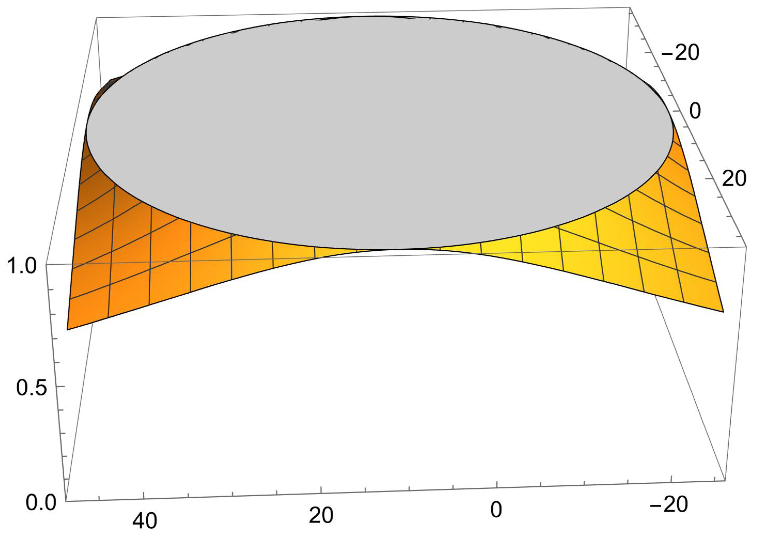
Figure 2.
Stability regions of and , in the complex plane.
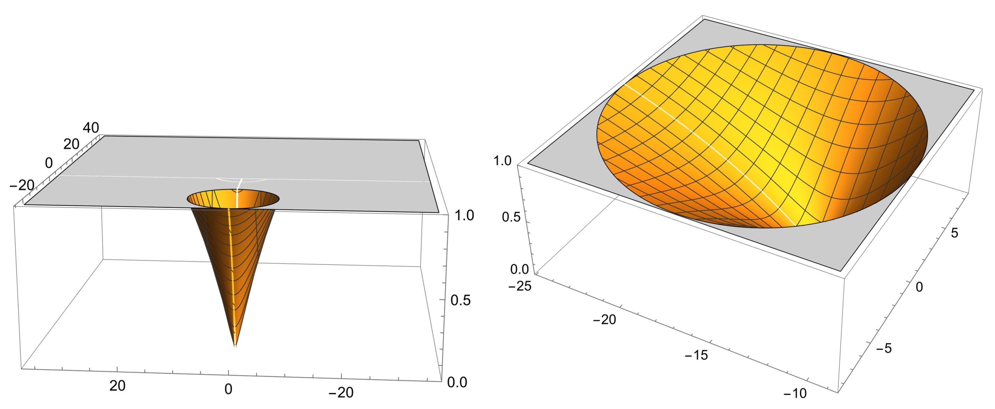
Figure 3.
Stability regions of for , in the complex plane.
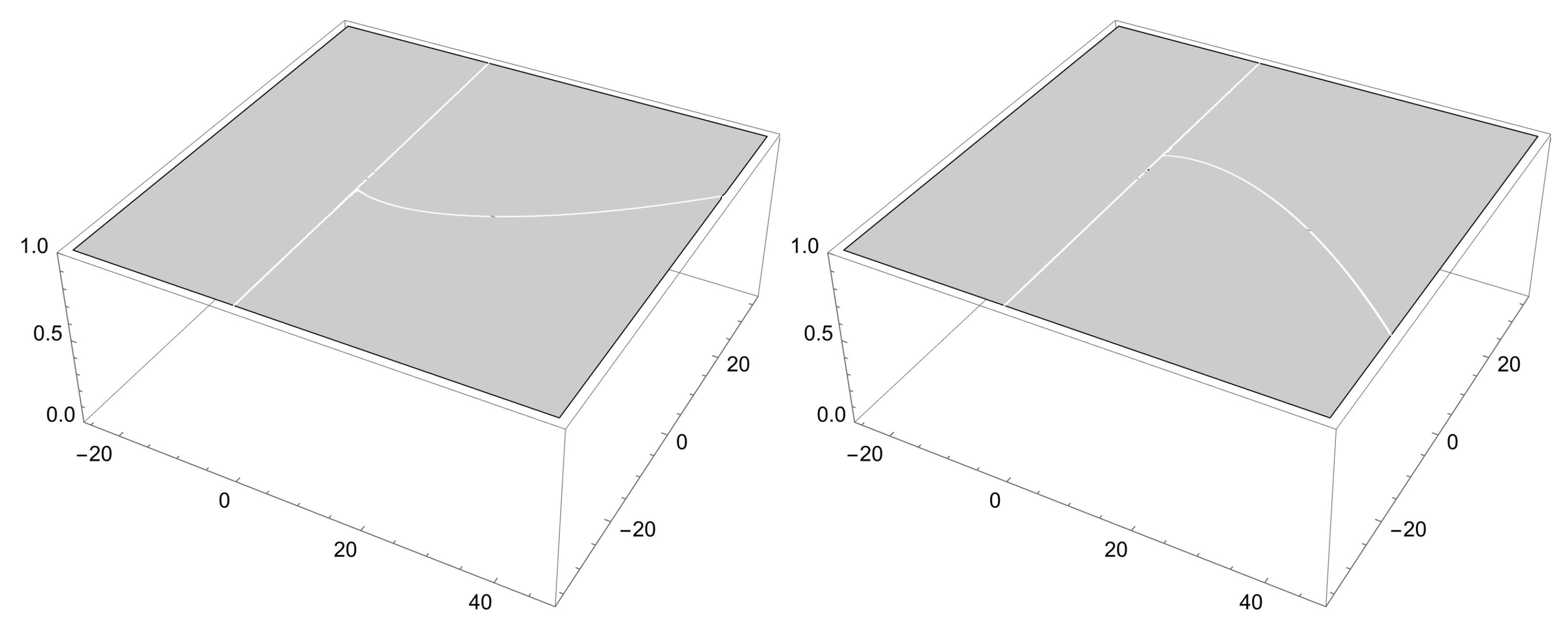
Figure 4.
Parameter planes corresponding to critical points , .
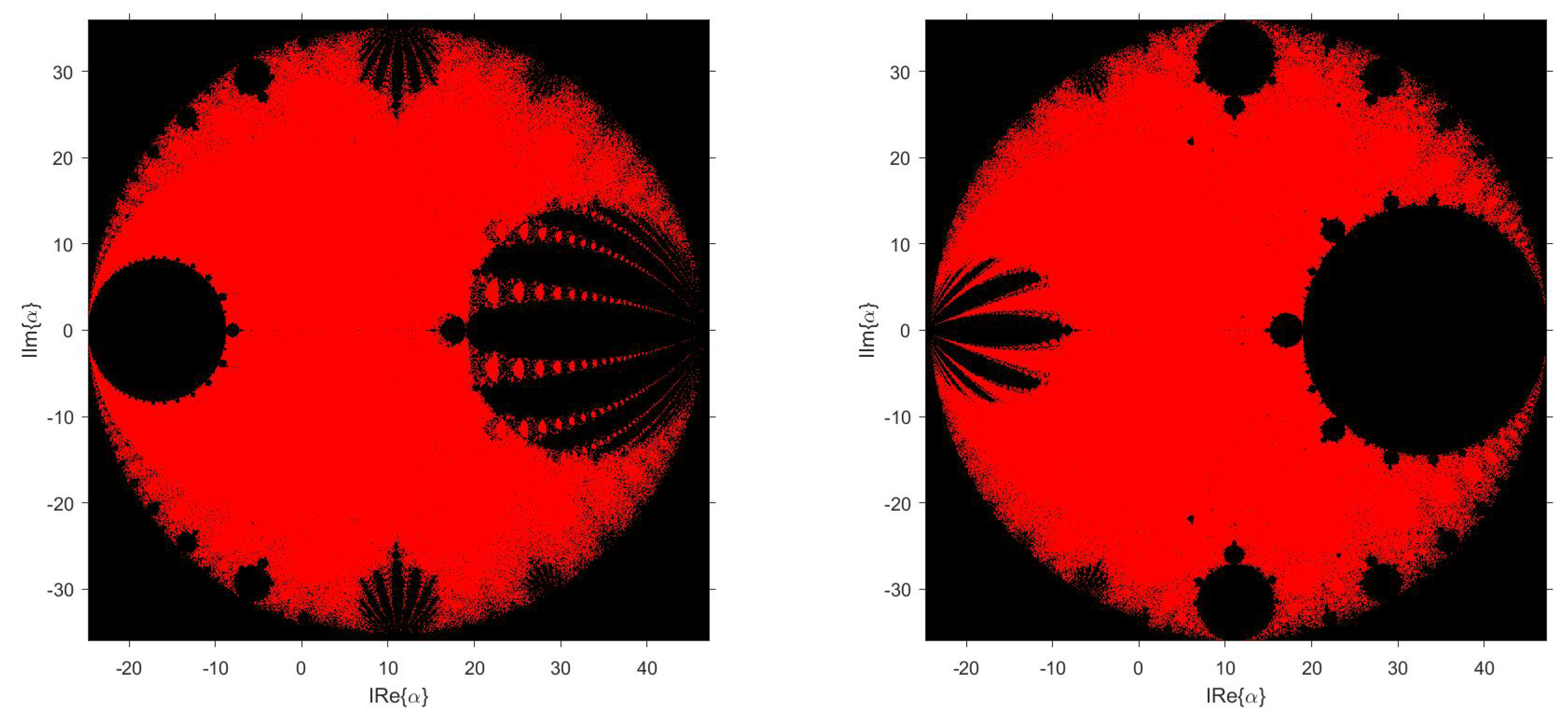
Figure 5.
Unified parameter plane.
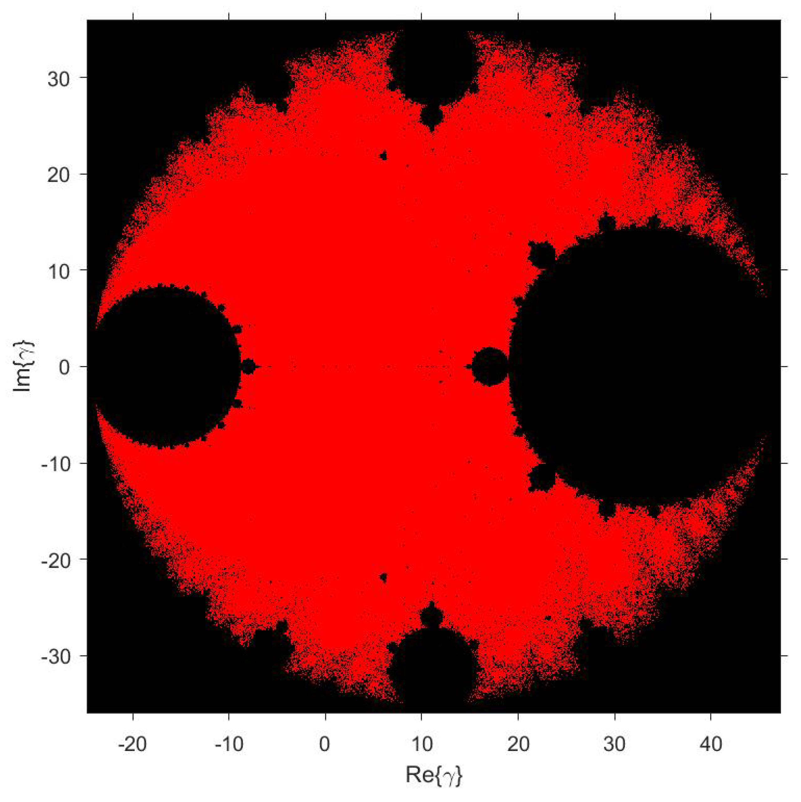
Figure 6.
Dynamical planes for stable and unstable values.
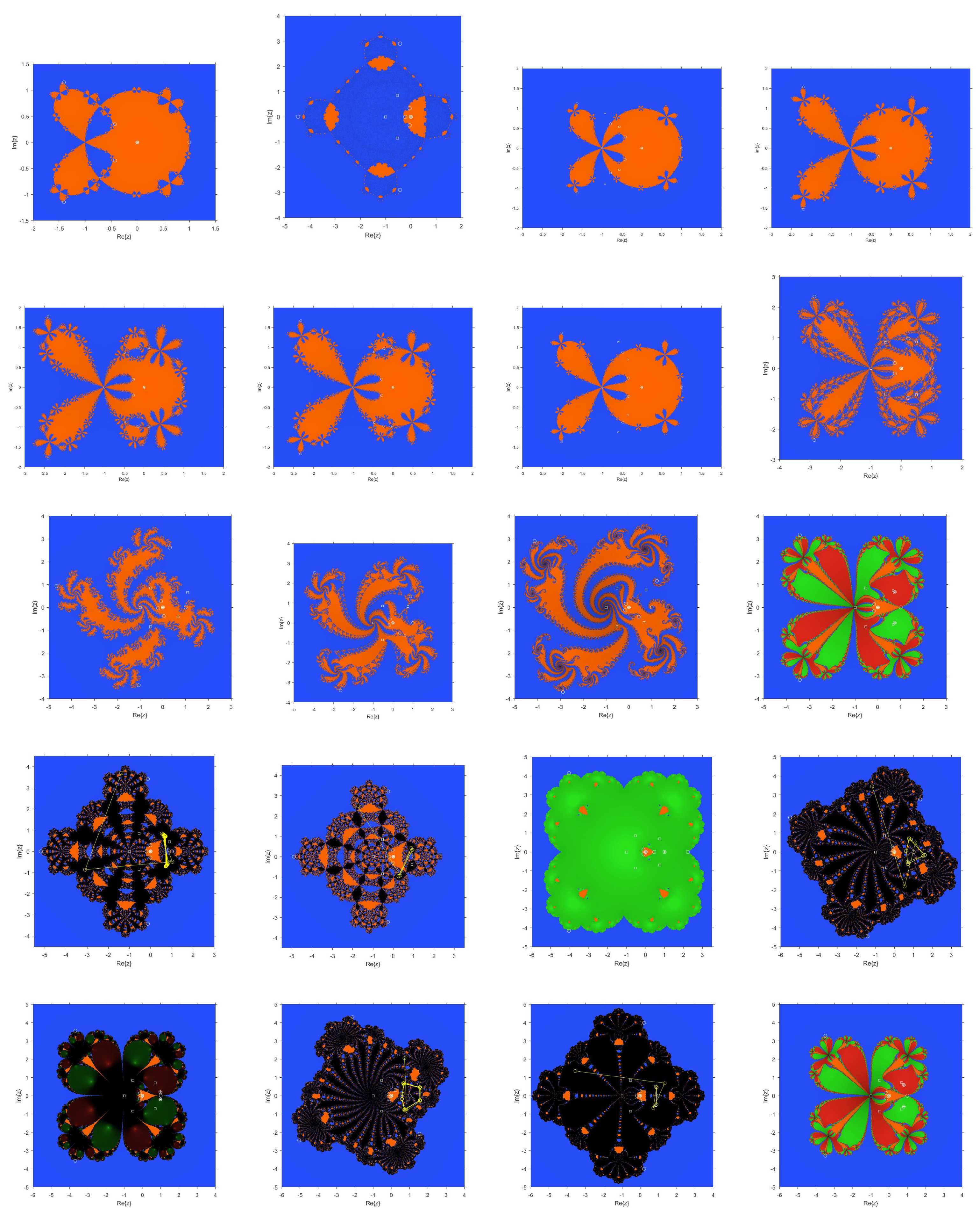

Table 1.
Degree of the polynomials whose zeros are free critical points of .
| Degree | Number of Families |
|---|---|
| 18 | 36 |
| 16 | 56 |
| 14 | 63 |
| 12 | 60 |
| 10 | 50 |
| 8 | 30 |
| 6 | 26 |
| 4 | 8 |
| 2 | 1 |
Table 2.
Values of related to parametric families where the degree (D) of the polynomial whose zeros are free critical points of the associated rational operator does not exceed 4 and their radius (r).
Table 2.
Values of related to parametric families where the degree (D) of the polynomial whose zeros are free critical points of the associated rational operator does not exceed 4 and their radius (r).
| r | D | ||
| 4 | |||
| 16 | 4 | ||
| 18 | 4 | ||
| 24 | 4 | ||
| 4 | |||
| 36 | 4 | ||
| 4 | |||
| 54 | 2 | ||
| 81 | 4 |
Table 3.
Stable and unstable values of .
| # RFP (∘) | # CP (□) | # AFP (∗) | Period | Stability | |
| 7 | 4 | 2 | 1 | Stable | |
| 8 | 5 | 2 | 1 | Stable | |
| 9 | 7 | 2 | 1 | Stable | |
| 7 | 3 | 2 | 1 | Stable | |
| 9 | 7 | 2 | 1 | Stable | |
| 9 | 7 | 2 | 1 | Stable | |
| 9 | 7 | 2 | 1 | Stable | |
| 9 | 7 | 2 | 1 | Stable | |
| 9 | 7 | 2 | 1 | Stable | |
| 9 | 7 | 2 | 1 | Stable | |
| 9 | 7 | 2 | 1 | Stable | |
| 9 | 7 | 4 | 1 | Unstable | |
| 9 | 7 | 2 | 2 | Unstable | |
| 9 | 7 | 2 | 2 | Unstable | |
| 9 | 7 | 3 | 1 | Unstable | |
| 9 | 7 | 2 | 4 | Unstable | |
| 9 | 7 | 4 | 1 | Unstable | |
| 9 | 7 | 2 | 4 | Unstable | |
| 9 | 7 | 2 | 2 | Unstable | |
| 9 | 7 | 4 | 1 | Unstable |
Table 4.
Number of iterations on test functions.
| Parameter Values | Stability | ||||
| 4 | 5 | 4 | 7 | Stable | |
| 4 | 100 | 4 | 100 | Stable | |
| 4 | 5 | 4 | 6 | Stable | |
| 4 | 5 | 4 | 6 | Stable | |
| 4 | 5 | 4 | 5 | Stable | |
| 4 | 4 | 4 | 5 | Stable | |
| 4 | 5 | 4 | 6 | Stable | |
| 4 | 6 | 4 | 6 | Stable | |
| 4 | 100 | 4 | 100 | Stable | |
| 4 | 64 | 4 | 100 | Stable | |
| 4 | 37 | 4 | 100 | Stable | |
| 4 | 100 | 4 | 100 | Unstable | |
| 4 | 100 | 4 | 100 | Unstable | |
| 4 | 100 | 4 | 100 | Unstable | |
| 4 | 59 | 5 | 100 | Unstable | |
| 4 | 100 | 4 | 100 | Unstable | |
| 4 | 100 | 4 | 31 | Unstable | |
| 4 | 100 | 4 | 44 | Unstable | |
| 4 | 100 | 4 | 100 | Unstable | |
| 4 | 100 | 4 | 11 | Unstable |
Table 5.
Comparative analysis on .
| Function | Method | Iter | Time | |||
|
|
Newton | 5 | 0.0713269 | 2 | ||
| Chun | 5 | 0.0927903 | 2 | |||
| Ostrowski | 5 | 0.0995647 | 2 | |||
| Kung-Traub | 5 | 0.1000585 | 2 | |||
| Jarratt | 4 | 0.0862121 | 4 | |||
| 4 | 0.0957585 | 4 | ||||
| 4 | 0.1063336 | 4 | ||||
| 4 | 0.0842142 | 4 | ||||
| 4 | 0.0909392 | 4 | ||||
| 4 | 0.0864402 | 4 | ||||
| 4 | 0.0856559 | 4 | ||||
| 4 | 0.0971327 | 4 |
Table 6.
Comparative analysis on .
| Function | Method | Iter | Time | |||
|
|
Newton | 7 | 0.0590956 | 2 | ||
| Chun | 6 | 0.0674999 | 2 | |||
| Ostrowski | 8 | 0.1065735 | 2 | |||
| Kung-Traub | 7 | 0.079534 | 2 | |||
| Jarratt | 5 | 0.0657351 | 4 | |||
| 5 | 0.0744865 | 4 | ||||
| 5 | 0.0720414 | 4 | ||||
| 5 | 0.071041 | 4 | ||||
| 5 | 0.069821 | 4 | ||||
| 4 | 0.0596417 | 4 | ||||
| 5 | 0.0698009 | 4 | ||||
| 6 | 0.1015708 | 4 |
Table 7.
Comparative analysis on .
| Function | Method | Iter | Time | |||
|
|
Newton | 5 | 0.0536364 | 2 | ||
| Chun | 6 | 0.0789598 | 2 | |||
| Ostrowski | 5 | 0.1089681 | 2 | |||
| Kung-Traub | 6 | 0.0912986 | 2 | |||
| Jarratt | 4 | 0.0626825 | 4 | |||
| 4 | 0.0754623 | 4 | ||||
| 4 | 0.0704758 | 4 | ||||
| 4 | 0.0670903 | 4 | ||||
| 4 | 0.0725264 | 4 | ||||
| 4 | 0.0794614 | 4 | ||||
| 4 | 0.0924925 | 4 | ||||
| 4 | 0.0739391 | 4 |
Table 8.
Comparative analysis on .
| Function | Method | Iter | Time | |||
|
|
Newton | 9 | 0.0776262 | 2 | ||
| Chun | 7 | 0.1032848 | 2 | |||
| Ostrowski | 7 | 0.1054047 | 2 | |||
| Kung-Traub | 7 | 0.1014812 | 2 | |||
| Jarratt | 5 | 0.0895486 | 4 | |||
| 7 | 0.1140201 | 4 | ||||
| 6 | 0.0925447 | 4 | ||||
| 6 | 0.1102584 | 4 | ||||
| 5 | 0.0844069 | 4 | ||||
| 5 | 0.0966304 | 4 | ||||
| 6 | 0.1174171 | 4 | ||||
| 6 | 0.1047413 | 4 |
Disclaimer/Publisher’s Note: The statements, opinions and data contained in all publications are solely those of the individual author(s) and contributor(s) and not of MDPI and/or the editor(s). MDPI and/or the editor(s) disclaim responsibility for any injury to people or property resulting from any ideas, methods, instructions or products referred to in the content. |
© 2023 by the authors. Licensee MDPI, Basel, Switzerland. This article is an open access article distributed under the terms and conditions of the Creative Commons Attribution (CC BY) license (http://creativecommons.org/licenses/by/4.0/).
Copyright: This open access article is published under a Creative Commons CC BY 4.0 license, which permit the free download, distribution, and reuse, provided that the author and preprint are cited in any reuse.


