Submitted:
11 December 2023
Posted:
12 December 2023
You are already at the latest version
Abstract
X-band marine radar captures signal reflected from the sea surface. Theoretical studies indicate that the initial unfiltered signal contains meaningful information including parameters related to wind waves. Traditional methods for estimating significant wave height (SWH) rely on the physical laws describing signal reflection from rough surfaces. However, recent studies suggest the feasibility of employing artificial neural networks (ANNs) for SWH approximation. Both classical and ANN-based approaches necessitate costly in situ data. In this study, we propose generating synthetic radar images with specified wind wave parameters using Fourier-based approach and Pierson–Moskowitz wave spectrum as a viable alternative. We generate synthetic images and use them for unsupervised learning approach to train a convolutional component of an ANN. After that, we train a regression ANN based on the previous convolutional component to obtain SWH back from synthetic images. Then, we apply preliminary trained weights for the same regression model to train SWH approximation on the dataset of real sea clutter images. In this study, we demonstrate the increase in the accuracy of SWH estimation from radar images with the preliminary training on synthetic data.
Keywords:
wind wave
; X-band marine radar
; significant wave height
; Pierson-Moskowitz spectrum
; synthetic radar images
; preliminary training
; artificial neural networks
; machine learning
; deep learning
; convolutional neural networks
; unsupervised pre-training
1. Introduction
The comprehensive examination of climate change involves the delineation of physical processes and interactions within the atmosphere-ocean system. Notably, the sea-wave interactions are strongly linked to surface wind speed and wind waves. Long-term climate reconstructions, such as the Global Atlas of the Ocean Waves [1], extensively utilize ocean wave parameters.
Marine X-band radars play an essential role in ship navigation and safety through the detection of obstacles. Besides their primary function, raw radar images capturing sea clutter contain substantive information. Analysis of the spatial distribution of the reflected signal facilitates the derivation of parameters associated with wind waves and swell. Additionally, these radar images allow estimating one of the vital sea surface characteristics – significant wave height (SWH).
The classical approach includes Fourier analysis and a linear dispersion relationship to recognize wave signals within the temporal series of radar data. The method necessitates the incorporation of modulation transfer functions and calibration coefficients specific to individual radar antennas [2], thereby constraining its generalizability. Despite this limitation, the classical methodology remains extensively applied for real-time estimation of ocean wave parameters, processing the back-scatter spectrum derived from radar images [3].
In addition to classical approach, radar data processing includes methodologies that are potentially faster and highly independent of radar antenna specifications. Notably, certain publications show superior significant wave height (SWH) estimation quality through contemporary artificial intelligence (AI)-based techniques [4], in comparison to classical methodologies. Within the machine-learning paradigm, the functional relationships, such as artificial neural networks (ANNs), between radar images and corresponding SWH values are approximated through training on extensive datasets. Consequently, the efficacy of the regression quality is correlated with the size and the distribution of the training dataset.
The authors in [5] address the challenge of limited data by employing an algorithm for generating synthetic radar images with arbitrary SWH value. This methodology uses technique of generating realistic ocean surfaces, as detailed in [6]. While the methodology in [5] does not incorporate image synthesis within a machine-learning framework, we hypothesize that the ANN model and synthetic datasets could potentially enhance the overall SWH estimation from real X-band real images.
Convolutional neural networks (CNNs) show their efficacy in image recognition and feature extraction across various scientific domains, including geosciences. A notable instance is illustrated in [7], where CNNs are employed for real-time SWH estimation utilizing a series of X-band radar images.
In summary, the recent progress in ANN and the emergence of modern machine-learning techniques have substantially diversified radar image processing methods. Nonetheless, the findings in this research domain present conflicting outcomes, and numerous questions persist. Consequently, evaluating current methodologies for radar image generation and SWH estimation remains a subject of ongoing scientific interest.
In this paper, we demonstrate the utilization of a preliminarily trained CNN for real marine X-band radar images of sea clutter for to estimate SWH. Initially, we elaborate the methodology of realistic radar images and generate a synthetic dataset. We train a model that reconstructs synthetic images in unsupervised learning approach. After that, we use preliminarily trained part of the reconstruction model to construct and train a regression model that approximates SWH from the synthetic image. Further, the pre-trained regression architecture is trained on a dataset of real radar images. We then compare the results of the pre-trained model with the quality of the simple SWH regression model.
The paper is organized as follows. In Section 2, we provide the details of the real radar image dataset, the methodology of the artificial radar image synthesis. and the architectures of the applied ANNs, quality metrics and training and evaluation procedures. In Section 3, we provide the results of the elaborated model training. In Section 4, we analyze how SWH estimation quality increases with pre-training on synthetic dataset. Concluding remarks are made in Section 5.
2. Materials and Methods
2.1. Initial Data
For this research, we adopt the data collection methodology outlined in [3]. Our dataset comprises samples obtained during four research expeditions conducted in the Atlantic and Arctic oceans. These expeditions were undertaken by the Shirshov Institute of Oceanology of the Russian Academy of Sciences within the governmental program of regular ocean observations.
The routes of the expeditions encompass points with SeaVision radar images and/or Spotter buoys measurements [8]. Comprehensive details about the research expeditions can be found in Table 1. The selection of locations for sea wave observation was based on local weather conditions and temporal constraints. As Table 1 illustrates, there are points without available Spotter buoy data. Consequently, for further study, we only utilize specific locations where simultaneous wind wave Spotter observations and SeaVision images were conducted. We denote such selected points by <<stations>>.
Spotter wave buoy provides highly accurate measurements of wind wave characteristics collecting the training dataset of SWH. SeaVision radar creates one sea clutter image every two seconds.
The center of the resulting sea clutter images coincides with the location of the radar antenna. Raw images with the spatial resolution of 1.875 m cover >7 km radius around the ship. The image exhibits a signal with diverse structures and intensities attributed to local wind direction, ship rotation, and reflections of electromagnetic signals from the rough ocean surface (e.g., [9]).
We suppose that each radar image includes an area with the most meaningful signal information about wave field. Additionally, there is a "blind" zone near the center due to signal reflection from the ship. To mitigate this effect, we exclude the part of the image within a 300-meter radius around the ship. Given that the reflected signal becomes less distinct with increasing distance from the radar antenna, we assume that a radius of ≈2000 meters ensures the highest significant variability observed in radar data. Consequently, first, we restrict our analysis to the 300–2000 meter range for further processing.
The important step of the data pre-processing is a choice of the optimal 180° sector containing the most informative wave signal. The technique used in this research extracts the most contrasting area from the entire radar image to provide the most clearly identified wind waves. For every station, the sector with the largest temporal standard deviation is the optimal sector. In this study, considering spatial resolution of 1.875 m, we choose the outer radius of the meaningful area as ≈1920 m (1024 px). Hence, we work with pre-processed images in contradistinction to in [3].
We linearly transform the values of the back-scattered radar signal image so that for every specific image, the minimum value is 0 and the maximum is 255. For further purposes, we use only masked real images. Namely, we replace the pixels outside 300–1920 meter radius area with zeros. The example of the pre-processed radar image is shown in Figure 1.
2.2. Synthesis of Realistic Sea Surface
We develop the methodology of generating realistic synthetic radar images [5] based on realistic ocean scenes [6]. The authors of [6] elaborated a technique that presents fully developed sea with an empirical modified Pierson-Moskowitz sea power spectrum [10].
As proposed in [6], we first generate a array with noise values uniformly distributed from to . We choose the image size that is bigger than 2048 to further exclude possible edge effects. The result of this step is a white-noise image (see Figure 2a).
We also assume that the spatial resolution is 1.875 m, equal to that of the real radar images. This parameter allows us to perform a two-dimensional forward Fourier transform of the white-noise image to generate an array of complex numbers. The magnitude of these complex Fourier components is shown in Figure 2b. The coordinate axes in Figure 2b are spatial frequencies and [].
In this research, we consider a simple case of fully developed wind waves, characterized by a wave power spectrum constant in time. Under these assumption, W. Pierson and L. Moskowitz [10] empirically approximated the mathematical form of the downwind power spectrum :
where f is the temporal frequency [Hz], is the peak temporal frequency [Hz], is the Phillips constant, and g is the mean gravitational acceleration [m/].
The form of the fully-developed wind spectrum (1) depends solely on a single parameter that indicates the frequency of the spectrum maximum. It was also discovered in [10] that is a function of 10 m surface wind speed :
SWH is usually defined as an average measurement of the largest 33% of waves [11]: , where N is the total number of measured waves, is a height of the j-th wave from the largest 33%. For a given power spectrum , we can equivalently calculate significant wave height [12]: . Thus, from (2), for Pierson-Moskowitz spectrum (1), we obtain:
Hence, we completely determine the shape of the one-dimensional downwind fully developed wave spectrum (1) with either or SWH (3).
The two-dimensional wave power spectrum was proposed in [13] as an extension of (1) taking the wind direction into account:
where is one-dimensional Pierson-Moskowitz spectrum from (1) and is a normalized directional multiplier at angle from the downwind direction. The empirical parameters in (5) are and that is equal to 4.06 for and –2.34 for .
The example of the normalized filter for =15 m/s for the frequency domain of Figure 2b is shown in Figure 3a. To transform the white-noise spectrum into the two-dimensional Pierson-Moskowitz spectrum (4), we multiply the magnitudes of the Fourier components of the initial white-noise image by (1) and (5).
The resulting spectrum creates a narrower profile near (2) in the downwind direction, forms a bimodal spectrum shape for from the downwind direction, and suppresses the long-crested peak frequency components, while retaining non-peak frequencies [6]. The filtered magnitudes of the white-noise Fourier components from Figure 2b are shown in Figure 3b.
Subsequently, we combine the filtered magnitudes with the original phase of the white-noise complex Fourier components, and apply the inverse Fourier transform, as described in [6]. The result of this procedure is a array of complex numbers. The desired synthetic sea surface is ar eal part of this array. We illustrate the full-domain realistic sea surface and its central part in Figure 4.
2.3. Synthesis of Radar Images
Here we describe transformation of the synthetic sea surfaces obtained in SubSection 2.2 into synthetic X-band radar images.
Two main geometrical effects that influence the X-band signal reflected from the sea surface are (1) shadowing and (2) tilt modulation [5]. We further follow the transformation technique proposed by [14] with the subsequent modifications [5].
Briefly, in this study, the shadowing effect refers to the geometrical optics approximation. In certain areas, the sea surface obstructs the reflection of radar rays from adjacent areas, leading to the shadowing of nearby waves. Consequently, the radar antenna receives no meaningful signal from the shadowed parts of the sea surface [5]. Obviously, this phenomenon depends on the grazing angle that is determined by the relationship between the radar antenna height and the distance to the antenna x (Figure 5).
For tilt modulation, the steepness of the observed surface slope affects the power amplitude received by the radar antenna [5]. Thus, for non-shadowed areas the received back-scattered signal is proportional to , where is the angle between the radar ray and the vector normal to the wave surface (Figure 5).
Summarizing, we present the following algorithm that transforms the synthetic sea surface into the realistic X-band radar image, For every synthetic sea surface:
- Distance mask: we determine the masked points – the points with the distance to the radar more than 1920 m or less than 300 m;
- Shadowing: we determine the points that are not available for a radar ray;
- Tilt modulation: for every non-shadowed point we determine the angle between the radar ray and the vector normal to the wave surface;
- For every non-shadowed point the amplitude of the back-scattered signal is ;
- We compute the minimum and the maximum values of the back-scattered amplitude among the non-shadowed points;
- Normalization: we linearly transform the amplitude values so that the new minimum value is 0 and the maximum value is 255;
- Noise: for shadowed and masked points we set the amplitude values as random numbers distributed uniformly from 0 to 255.
- We choose the half of the array that corresponds to the downwind direction.
The resulting synthetic X-band radar image with size is shown in Figure 6.
2.4. Dataset of Synthetic Images
To generate a set of synthetic images, we first generate 60,000 values of speed distributed uniformly in the range from 3 m/s to 20 m/s. We include extremely low and extremely high wind speed values to provide proper learning quality in comparison with the real wind wave conditions. For fully-developed sea, SWH value is a quadratic function of (3) leading to a bigger share of lower SWH values. The distributions of and SWH are shown in Figure 7.
After that, for every wind speed value we generate a corresponding sea surface, as described in SubSection 2.2, and then convert it to a synthetic radar image, according to SubSection 2.3. We compute the grazing angles assuming that the radar antenna height m. This procedure results in 60,000 samples of synthetic radar images. Illustrative cases for various values of wind speed are presented in Figure 6.
2.5. Data Pre-Processing
In this research, we apply convolutional neural networks (CNNs). Consistent with standard practice, we linearly normalized both input data and the target SWH values, adjusting them to approximately have a zero mean and a variance equal to one. Namely, for every pixel x of the real and synthetic radar images, the normalized radar image pixel . Nevertheless, after normalization, for the masked areas of the image (white areas in Figure 6a), we set the zero value. The normalized target value is .
CNNs lack inherent rotation invariance, necessitating diverse training data with varied spatial feature orientations to achieve rotation invariance. In this study, we assume that the orientation of spatial features may not exhibit high diversity. Consequently, we employ two-dimensional data augmentation fir the real SeaVision and synthetic radar semicircles, namely, random rotation with an angle ranging from -5° to 5°. This approach encourages the CNN-based model to acquire rotation invariance through training on augmented data, thereby enhancing the generalization ability of the CNN.
2.6. ANN Models
In this study, we apply convolutional neural networks (CNNs), i.e., parametric mappings where the model parameters are optimized through sequential application of a fixed-size convolutional kernel to two-dimensional input data [15].
The high depth of CNNs is anticipated to enhance the predictive output quality. However, the large number of layers introduces training instability in the back-propagation algorithm, leading to learning inefficiency due to the <<vanishing gradients>> effect. This effect results from the accumulation of excessively small gradients for model parameters. Consequently, the product of the gradient vector and the learning rate coefficient tends toward zero, causing the parameters to remain constant during each optimization step.
An effective approach to address the issue of learning instability involves the incorporation of connections that bypass the intermediate layers of the model. These skip connections serve to diminish the likelihood of accumulating small gradients. A notable example is the implementation of residual connections, wherein the output of an intermediate layer is added to the output of a subsequent level.
In this paper, we build two CNN architectures based on the model for processing SeaVision radar images as it is described in [16]. The basic architecture is the modified ResNet50 combining the advantages of deep CNNs and residual connections.
The convolutional core of the modification adheres to the original ResNet architecture, with the addition of sinusoidal positional encoding of various wavelengths to enable the CNN to capture the wavelengths peculiar to real SeaVision images [16]. Two-dimensional positional encoding introduces additional channels with generated harmonic maps featuring various wavelengths and directions. Specifically, there are cosine- and sine-based positional encoding channels that vary in both horizontal and vertical directions. These maps are concatenated with the output of the ResNet blocks so that the subsequent ResNet block processes activation maps from the previous layers along with the positional encoding channels. It is worth noting that for modified ResNet50, positional encoding maps are injected into the activation maps after each ResNet building block.
2.6.1. Unsupervised Reconstruction Model
The first architecture elaborated for this research is the reconstruction CNN model with the structure similar to U-Net [17]. U-Net is based on a typical contracting network augmented with consecutive upsampling blocks. Hence, U-Net architecture consists of two parts: the contracting path from the input to the bottleneck, and the expansive path from the bottleneck to the output. The upsampling blocks of the model contain a large number of feature channels to effectively propagate context information to higher resolution layers.
The main distinction and the principal concept of U-Net is the presence of the specific skip connections that transmit activation maps from the intermediate layers of the contracting path to the intermediate layers of the expansive path. In other words, the high-resolution features from the contracting path are added to the upsampled output on the expansive path to facilitate localization. Subsequently, a consecutive convolution layer is capable of learning to generate a more precise output based on this information [17].
For this research, we develop a U-Net architecture with the contracting path based on the convolutional core of modified ResNet50 (the upper half of Figure 9). The input of the model is supposed to be a two-dimensional array with size. Four skip connections and a bottleneck pass the multilevel features into the expansive path of the model (the lower half of Figure 9). It leads to the output with the input size. With the equal size of the input and the output, the model architecture is aimed at unsupervised reconstruction of the input array.
As Figure 9 shows, the expansive part of the model consists of ResNet pr upsampling ResNet blocks with the additional upsampling layers if necessary. On the expansive path, we coordinate the spatial size of the block outputs with the outputs of the skip connections to properly concatenate the tensors before the subsequent ResNet block or layer. The number of channels for the concatenated activation maps and the output size of the skip connections are shown in Figure 9.
2.6.2. Regression Model
The second architecture built for this study is the regression CNN model designed to approximate the scalar target SWH value through processing radar images. Unlike the regression model from [16] with the same input and output objects, we base our model on the reconstruction architecture described in Section 2.6.1 including the skip connections (see Figure 10).
As Figure 10 shows, our regression model consists of four fundamental parts. The first part is the convolutional core of modified ResNet50. We preserve four contracting paths to pass the outputs of the intermediate layers to the downsampling blocks. Every parallel downsampling block consists of a pooling layer, a convolutional layer, a pixel unshuffling layer and two consecutive convolutions. The task of the downscaling part of the model is to bring four activation maps of the skip connections to the same size. In the third part of the architecture, the features from the previous block are aggregated through channel concatenation. The aggregated activation map is passed to the downsampling block resulting in vector of size 64. The fully-connected subnet following the aggregation part contains two sequential fully-connected layers of the widths 64 and 8. The terminating layer is of the width 1 since in this study, we approximate SWH scalar.
2.7. Quality Metrics
Various quality metrics are employed to assess and monitor the learning process of the models. For the unsupervised reconstruction model, the simplest quality metric utilized is the root mean-squared error, denoted as . This form of reconstruction error quantifies the disparity between the input data and the data obtained after the U-Net compresses and decompresses the input. The metric provides an evaluation of the noise introduced to the input as it passes through the bottleneck and the skip connections.
If we denote our reconstruction model as R and a batch of input images as y, then an output batch is . We compute summarizing only by unmasked points to exclude non-meaningful areas of radar images. The number of points in the input batch is N, and the result is:
In (6), and are the identical elements of the input and the output tensors. We summarize the difference between the input and the output point-by-point. The indices i, j and k are in ranges of respective spatial dimensions and a batch size, taking into account distance mask.
The inadequacy of RMSE in detecting visually altered defective regions in images with consistent intensity values has been demonstrated [18]. In this research, we adopt a perceptual quality metric grounded in structural similarity, which assesses the inter-dependencies among local image regions. Unlike RMSE, which compares pixel values, structural similarity takes into account contrast and structural information. The computation of the structural similarity index measure (SSIM) is outlined as follows:
where is the pixel sample mean of y, is the pixel sample mean of , is the variance of y, is the variance of , is the cross-correlation of y and . and are constant values equal to and , respectively.
In this paper, we compute the Structural Similarity Index (SSIM) between two windows, each sized 128 px × 128 px, applied to both the input and the output images. The SSIM values range between and 1, where a higher SSIM signifies greater similarity.
In case of the regression model, only root mean-squared error is utilized since the output of this CNN is a vector containing significant wave height values with a length equal to the batch size :
where is a target value measured by Spotter buoy (see Section 2.1) or determined by the synthetic ocean surface (see Section 2.2), and is the output value of the regression model.
2.8. Training and Evaluation
The training process of artificial neural networks is known for its sensitivity to various details, and the selection of a training algorithm and hyperparameters plays a critical role in determining the quality of the resulting model. Currently, the Adam optimizer [19] stands out as the most stable and widely employed training algorithm, utilizing a momentum approach to estimate lower-order moments of the loss function gradients. In our study, we leverage the Adam optimization procedure.
In the optimization algorithms, the batch size and the learning rate hold particular significance. Due to the substantial dimensions of SeaVision radar images, substantial variations in batch size were impractical. Instead, we selected the largest feasible batch size for our computer hardware (batch_size=2) to mitigate noise in CNN gradient estimates. Adhering to best practices, we fine-tuned the learning rate schedule not only to attain high quality in SWH regression but also to enhance robust generalization skills. Generalization is evaluated by scrutinizing the disparity between the quality estimated on the training and validation subsets, where a small gap signifies good generalization and a large gap indicates poor generalization.
Aligned with recent research findings, we implemented the specialized learning rate schedule. This cyclical schedule encompasses a cosine-shaped decrease in the learning rate throughout the training process. We incorporate a multiplicative form of increase in the simulated annealing period with each cosine cycle. We also employ exponential decay of the simulated annealing magnitude with each cosine cycle, utilizing the multiplicative form.
In this research, training consists of three principal consecutive steps. For all the steps, we use normalized values as it was described in Section 2.3.
On step One, we train the reconstruction model using the dataset of synthetic images described in Section 2.4. The dataset comprising 60,000 synthetic radar images is randomly divided into two segments: a training dataset (50,000 images) and a validation dataset (10,000 images).
In machine learning, it is customary to assess the performance of a model by computing quality metrics on a validation subset obtained through random sampling from the original set of labeled examples. This methodology presupposes that the examples are independent and identically distributed (i.i.d.). The random partition ensures a uniform distribution of modeled surface wind wave conditions across the datasets. Moreover, the distribution of SWH values are similar for both datasets.
We train the reconstruction model using the mean-squared error between an input and an output images summing only over unmasked points. The length of training is 80 epochs. The learning rate schedule for the reconstruction model is in Figure 11. We change the first cosine cycle from learning_rate to learning_rate.
On step Two, we train the regression model using the same dataset of synthetic images described in Section 2.4. The number of images for training and evaluation is the same as for step One. Nevertheless, we change the random split of the dataset to prevent overfitting.
Step Two consists of two stages: and . For both stages of step Two, the input of the model is the masked radar image. We train the regression model using the mean-squared error between an output value and a target SWH.
For stage , we initialize the weights of the convolutional modified ResNet50 core and the skip connections with the weights from the pre-trained reconstruction model as described for step One. After that, we train only downsampling block, feature aggregation and fully-connected layers. The covolutional core weights are frozen. After 20 epochs, we start stage , training the full regression model. Epoch 1 of stage is inintialized with the weights of the full regression model after epoch 20 of stage . The length of stage training is 40 epochs. The learning rate schedule for step Two is in Figure 12. We change the cosine cycles from learning_rate to learning_rate.
In investigations concerning the application of statistical models, particularly ANNs, for the analysis of remote sensing data, it is crucial to account for the autocorrelation inherent in the observational time series dataset. Owing to the inherent evolution of underlying physical phenomena, consecutive observations may demonstrate substantial autocorrelation, thereby influencing the accuracy of the model [16].
On step Three, we train the regression model using the dataset of real SeaVision synthetic images described in Section 2.1.
It is imperative to refrain from systematically incorporating consecutive examples into the training and testing sets. In this research, we tackle the challenge of strongly correlated successive examples by adopting station-wise random sampling, a strategy akin to the one employed in [16]. This approach avoids the systematic sampling of successive examples into the training and validation subsets, ensuring a reliable assessment of our model’s quality.
Step Two consists of three stages: , and . The input of the model is the masked radar image. We train the regression model using the mean-squared error between an output value and a target Spotter buoy SWH.
For stage , we initialize the weights of the full model with the weights from the pre-trained regression model after stage . Then, we train only fully-connected block for 10 epochs. After that, on stage we start training fully-connected block, feature aggregation and downsampling block while the covolutional core weights are frozen. After 40 epochs of stage , we start stage , training the full regression model. The length of stage training is 20 epochs. The learning rate schedule for step Two is in Figure 13. We change the cosine cycles from learning_rate to learning_rate for stages and , and from learning_rate to learning_rate for stage .
3. Results
In this section, we present the results of three steps of estimating SWH from SeaVision radar imagery including pre-training in synthetic radar images.
The unsupervised reconstruction training shows relatively high (i.e., relatively good) Structural Similarity Index value on validation dataset. This result means that the reconstruction model is able to extract the multi-level features from the synthetic radar images. The convolutional core passes the extracted and processed features through the skip connection. This detail of the architecture allows subsequent use of step One weights for step Two.
The regression model trained on the synthetic dataset (step Two) demonstrates root mean-squared values m after stage and m after stage on validation dataset. The monotonous decrease in RMSE value proves the necessity for gradual unfreezing of pre-trained weights for smooth transition from the previous step. These values of are too good to be true in case of real-world data, however, one may consider them as the measure of success in case of synthetic dataset. These low (i.e., good) values of indicate that the neural network is capable of handling the variety of imagery similar to radar-captured sea clutter images.
The regression model trained on the synthetic dataset (step Three) show root mean-squared values m after stage , m after stage and m after stage on validation dataset.
We compare the final results in our study with the simple modified ResNet50 without pre-training [16]. As one may see, pre-training with synthetic data and architecture modifications proposed in our study significantly improves he quality of SWH approximation in terms of root mean-squared error: from m reported in [16] to m.
4. Discussion
This study initially proposes the efficacy of neural-network regression methods for determining SWH from sea clutter imagery acquired by a navigation X-band radar. However, in situ data collection is both costly and limited in its ability to offer a diverse range of ocean wave conditions.
The synthesis of radar images effectively addresses the issue of insufficient data. Moreover, the generation of diverse synthetic sea surface conditions allows for simulating radar images with specific hyperparameters essential for the research. Synthetic images contribute to the expansion of the dataset, rendering it in a more uniform manner.
We present an enhanced approach for generating a synthetic sea surface and synthetic radar images under the condition of a fully-developed sea. We suppose this method promising as it allows for the utilization of various power spectra of wind waves. The resulting images exhibit realism for visual perception.
Recent studies demonstrate proficiency in the task of SWH approximation, particularly in cases of low wind speed. To enhance CNN generalization capabilities, we developed two different architectures capable of proper preliminary training to conduct experiments involving the unsupervised reconstruction and the regression model on an elaborated synthetic dataset.
The results of the unsupervised reconstruction illustrate that the U-net-like model with skip connections and ResNet blocks is capable of capturing the harmonic structure of wind waves.
Our findings indicate that the autoencoder struggles in reconstructing fine structure of ocean wind waves. In the light of this circumstance, we suggest that the Mean Squared Error (MSE) training loss, which is sensitive to point-by-point distortions, tends to smooth images and eliminate small-scale features. At the same time, it is precisely the small-scale structure of an imagery that encompasses crucial information about wave lengths and heights. Consequently, the pre-trained ResNet-50, which loses wave information, exhibits a regression quality inferior to the initial expectations.
5. Conclusions and Outlook
In this study, we demonstrate the capability of a convolutional neural network (CNN) we propose in this paper of approximating significant wave height (SWH) with the quality superior to the one reported in recent studies exploiting CNNs in this task [16]. The superiority is achieved through the preliminary training of our CNN within the subsequent stages of (a) unsupervised autoencoder-like training and (b) further supervised pre-training with a synthetic target of the sense similar to the real SWH. We demonstrate significant improvement of the SWH estimation quality in terms of root mean squared error, compared to the results reported recently in a similar CNN-involving setting [16].
Synthetic dataset simulating radar-acquired sea clutter imagery with corresponding SWH values that we used in our pre-training may provide additional improvements for an utilized artificial neural network due to the control over the distribution of both wind speed values and corresponding SWH values.
Author Contributions
Conceptualization, Mikhail Krinitskiy and Natalia Tilinina; Data curation, Alexander Gavrikov and Alexander Suslov; Formal analysis, Alexander Gavrikov; Funding acquisition, Natalia Tilinina; Methodology, Mikhail Krinitskiy and Viktor Golikov; Project administration, Mikhail Krinitskiy and Natalia Tilinina; Resources, Mikhail Krinitskiy; Software, Vadim Rezvov, Viktor Golikov and Mikhail Borisov; Supervision, Mikhail Krinitskiy; Validation, Alexander Gavrikov and Mikhail Borisov; Visualization, Vadim Rezvov, Viktor Golikov and Alexander Suslov; Writing – original draft, Vadim Rezvov; Writing – review & editing, Mikhail Krinitskiy. All authors have read and agreed to the published version of the manuscript.
Funding
This research was funded by the program PRIORITY 2030 of Moscow institute of Physics and Technology.
Data Availability Statement
The data presented in this study are openly available in through the PANGAEA repository at https://doi.org/10.1594/PANGAEA.939620.
Conflicts of Interest
The authors declare no conflict of interest.
Abbreviations
The following abbreviations are used in this manuscript:
| MDPI | Multidisciplinary Digital Publishing Institute |
| DOAJ | Directory of open access journals |
| TLA | Three letter acronym |
| LD | Linear dichroism |
References
- Global Atlas of Ocean Waves. Available online: http://www.sail.msk.ru/atlas/ (accessed on 6 December 2023).
- Nieto-Borge, J.C.; Hessner, K.; Reichert, K. Estimation of the significant wave height with X-band nautical radars. In Proc. 18th Int. Conf. Offshore Mechanics and Arctic Engineering (OMAE), 1999.
- Tilinina, N.; Ivonin, D.; Gavrikov, A.; Sharmar, V.; Gulev, S.; Suslov, A.; Fadeev, V.; Trofimov, B.; Bargman, S.; Salavatova, L.; Koshkina, V.; Shishkova, P.; Ezhova, E.; Krinitsky, M.; Razorenova, O.; Koltermann, K.P.; Tereschenkov, V.; Sokov, A. Wind waves in the North Atlantic from ship navigational radar: SeaVision development and its validation with the Spotter wave buoy and WaveWatch III. Earth Syst. Sci. Data 2022, 14, 3615–3633. [Google Scholar] [CrossRef]
- Vicen-Bueno, R.; Lido-Muela, C.; Nieto-Borge, J.C. Estimate of significant wave height from non-coherent marine radar images by multilayer perceptrons. EURASIP J. Adv. Signal Process. 2012, 84. [Google Scholar] [CrossRef]
- Ludeno, G.; Serafino, F. Estimation of the Significant Wave Height from Marine Radar Images without External Reference. J. Mar. Sci. Eng. 2019, 7, 432–443. [Google Scholar] [CrossRef]
- Mastin, G.A.; Watterberg, P.A.; Mareda, J.F. Fourier Synthesis of Ocean Scenes. IEEE Comput. Graphics Appl. 1987, 3, 16–23. [Google Scholar] [CrossRef]
- Choi, H; Park, M.; Son, G.; Jeong, J.; Park, J.; Mo, K.; Kang, P. Real-time significant wave height estimation from raw ocean images based on 2D and 3D deep neural networks. Ocean Engineering 2020, 201. [Google Scholar] [CrossRef]
- Spotter Buoy by Sofar. Available online: https://www.sofarocean.com/products/spotter (accessed on 7 December 2023).
- Lyzenga, D.R.; Walker, D.T. A Simple Model for Marine Radar Images of the Ocean Surface. IEEE Geoscience and Remote Sensing Letters 2015, 12, 2389–2392. [Google Scholar] [CrossRef]
- Pierson, W.; Moskowitz, L. A proposed spectral form for fully developed wind seas based on the similarity theory of S. A. Kitaigorodskii. J. Geophys. Res. 1964, 69, 5181–5190. [Google Scholar] [CrossRef]
- Significant Wave Height. Available online: https://www.weather.gov/mfl/waves (accessed on 8 December 2023).
- NDBC – How are significant wave height, dominant period, average period, and wave steepness calculated? In Available online:. Available online: https://www.ndbc.noaa.gov/faq/wavecalc.shtml (accessed on 8 December 2023).
- Hasselmann, D.E.; Dunckel, M.; Ewing, J.A. Directional Wave Spectra Observed during JONSWAP 1973. J. Phys. Oceanogr. 1980, 10, 1264–1280. [Google Scholar] [CrossRef]
- Nieto Borge, J.; RodrÍguez, G.R.; Hessner, K.; González, P.I. Inversion of Marine Radar Images for Surface Wave Analysis. Journal of Atmospheric and Oceanic Technology 2004, 21, 1291–1300. [Google Scholar] [CrossRef]
- Rezvov, V.; Krinitskiy, M.; Gulev, S. Approximation of high-resolution surface wind speed in the North Atlantic using discriminative and generative neural models based on RAS-NAAD 40-year hindcast. In The 6th Int. Workshop on Deep Learning in Computational Physics, Russia, 2022; p. 429.
- Krinitskiy, M.A.; Golikov, V.A.; Anikin, N.N.; Suslov, A.I.; Gavrikov, A.V.; Tilinina, N.D. Estimating Significant Wave Height from X-Band Navigation Radar Using Convolutional Neural Networks. Moscow University Physics Bulletin 2023, accepted. [Google Scholar] [CrossRef]
- Ronneberger, O.; Fischer, P.; Brox, T. U-net: Convolutional networks for biomedical image segmentation. In Medical Image Computing and Computer-Assisted Intervention–MICCAI 2015: 18th International Conference, Munich, Germany, 5–9 October 2015; pp. 234–241.
- Bergmann, P.; Löwe, S.; Fauser, M.; Sattlegger, D.; Steger, C. (2018). Improving unsupervised defect segmentation by applying structural similarity to autoencoders. arXiv 2018, arXiv:1807.02011. [Google Scholar]
- Kingma, D.P.; Ba, J. Adam: A method for stochastic optimization. arXiv 2014, arXiv:1412.6980. [Google Scholar]
Figure 1.
The example of the pre-processed radar image from AI57 marine research mission of Institute of Oceanology of Russian Academy of Sciences.The position of a radar antenna is in point.
Figure 1.
The example of the pre-processed radar image from AI57 marine research mission of Institute of Oceanology of Russian Academy of Sciences.The position of a radar antenna is in point.
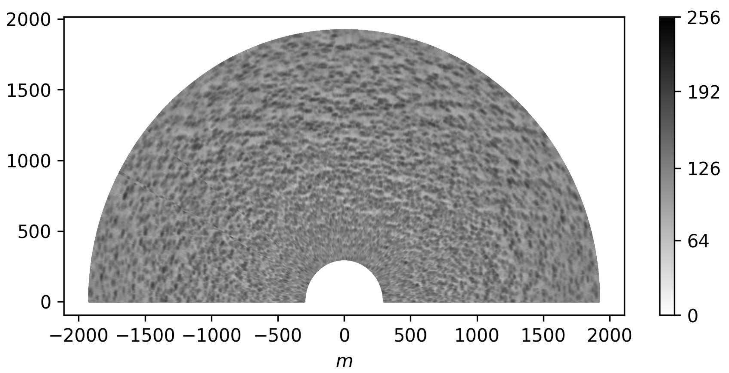
Figure 2.
The first stage of the sea surface synthesis: (a) White noise; (b) Fourier-transformed white noise
Figure 2.
The first stage of the sea surface synthesis: (a) White noise; (b) Fourier-transformed white noise
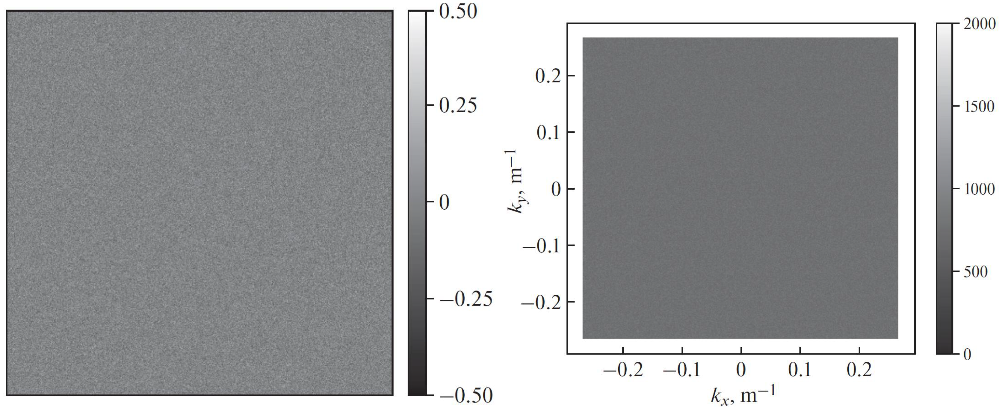
Figure 3.
The second stage of the sea surface synthesis: (a) Two-dimensional spectral filter (=15 m/s) for white-noise Fourier components; (b) Filtered magnitudes of white-noise Fourier components
Figure 3.
The second stage of the sea surface synthesis: (a) Two-dimensional spectral filter (=15 m/s) for white-noise Fourier components; (b) Filtered magnitudes of white-noise Fourier components
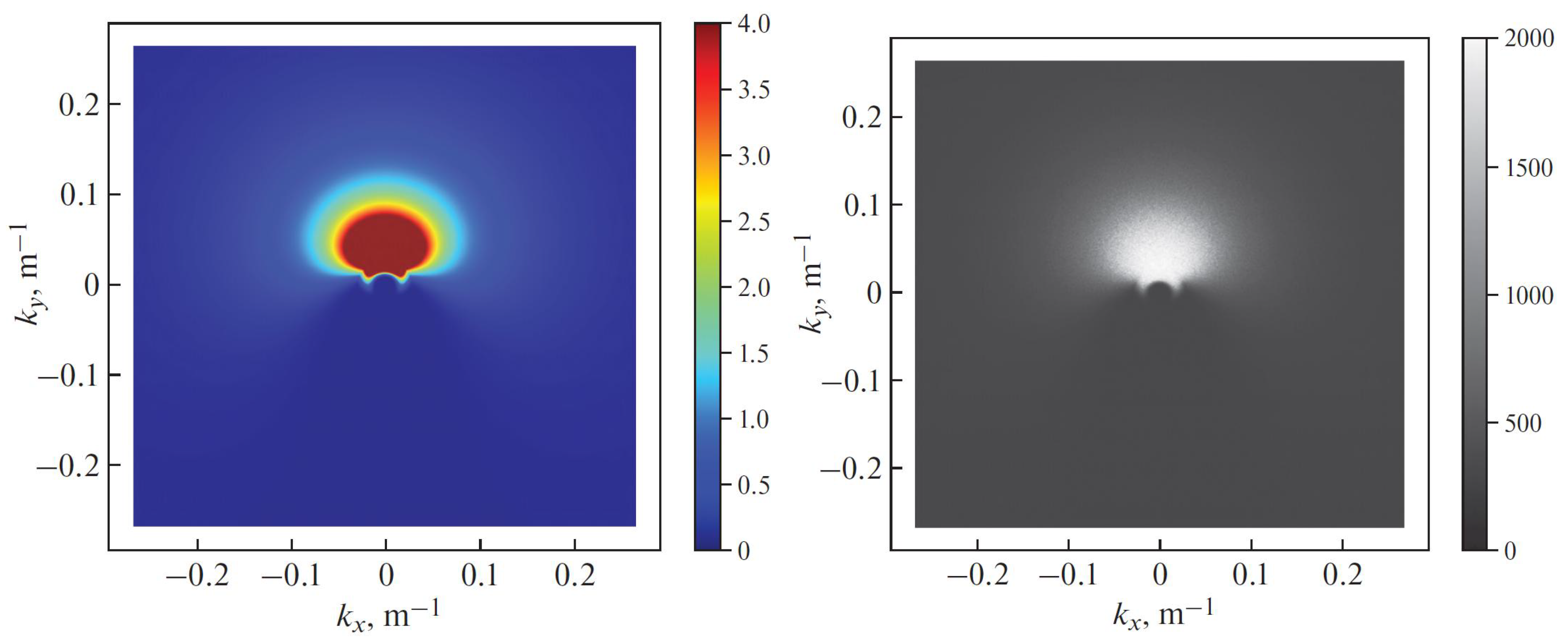
Figure 4.
The synthetic sea surface created by processing the white-noise image from Figure 2a: (a) Full image; (b) 200 m × 200 m area
Figure 4.
The synthetic sea surface created by processing the white-noise image from Figure 2a: (a) Full image; (b) 200 m × 200 m area
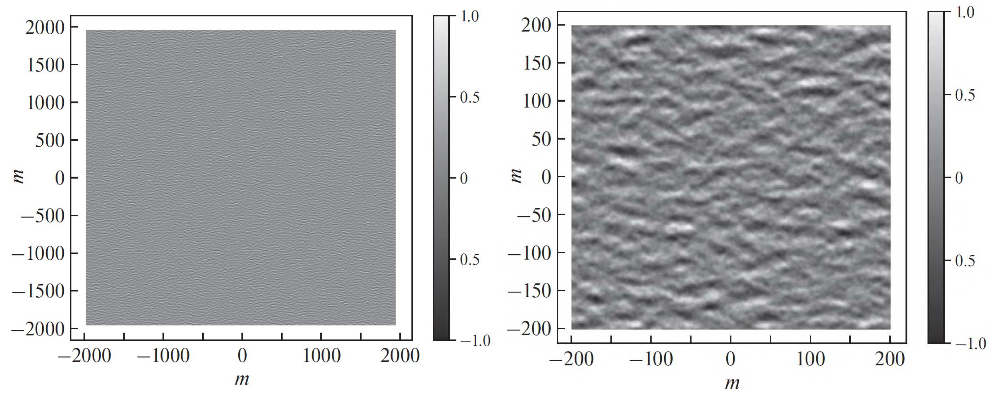
Figure 5.
Geometrical scheme of shadowing and tilt modulation effects [5].
Figure 5.
Geometrical scheme of shadowing and tilt modulation effects [5].
Figure 6.
The synthetic X-band radar image: (a) without the mask; (b) masked
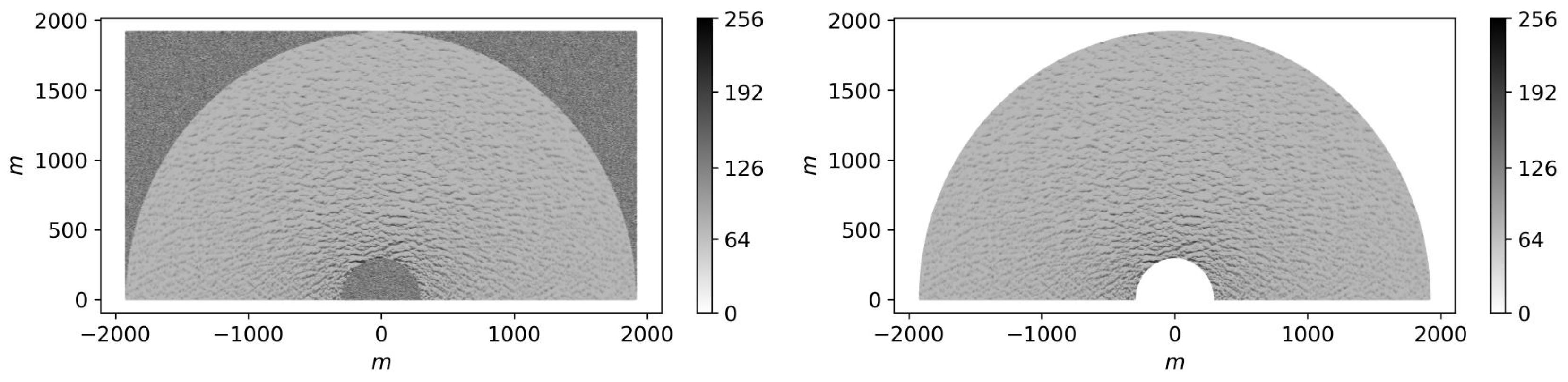
Figure 7.
The statistical distribution of the synthetic radar dataset: (a) wind speed; (b) SWH
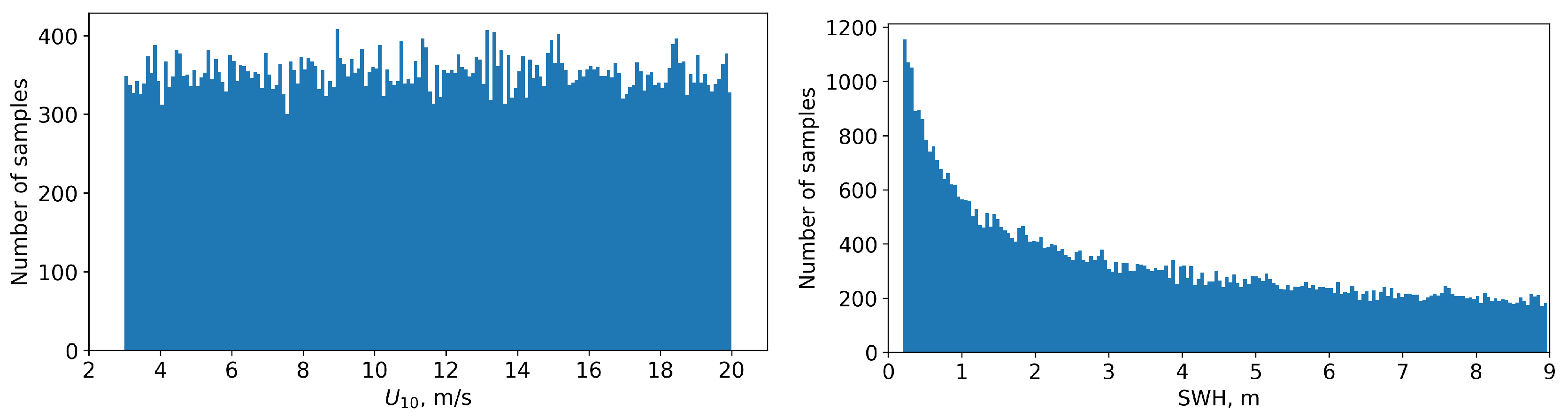
Figure 8.
The examples of synthetic radar images with different wind speed: (a) 4 m/s; (b) 12 m/s; (c) 20 m/s.
Figure 8.
The examples of synthetic radar images with different wind speed: (a) 4 m/s; (b) 12 m/s; (c) 20 m/s.
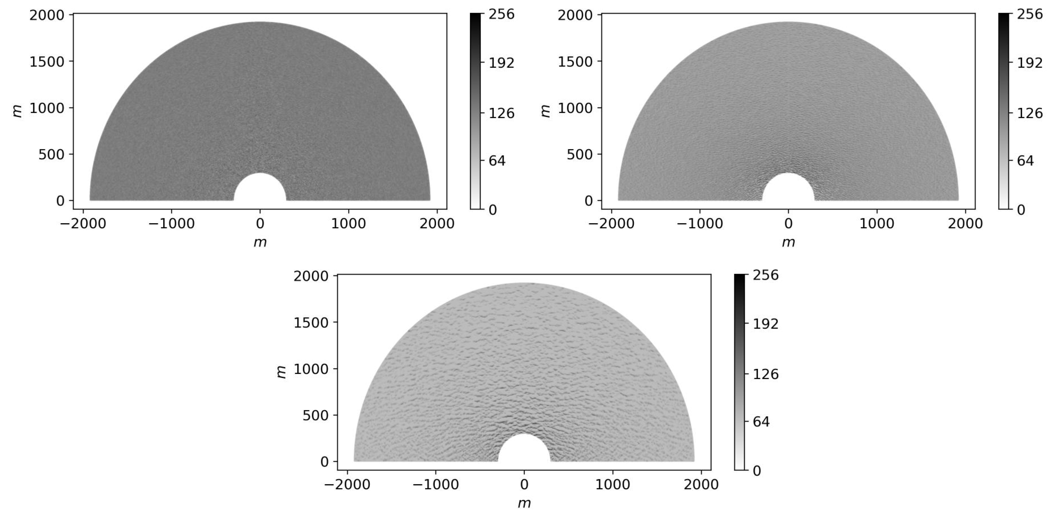
Figure 9.
High-level architecture of the reconstruction CNN model based on modified ResNet50.
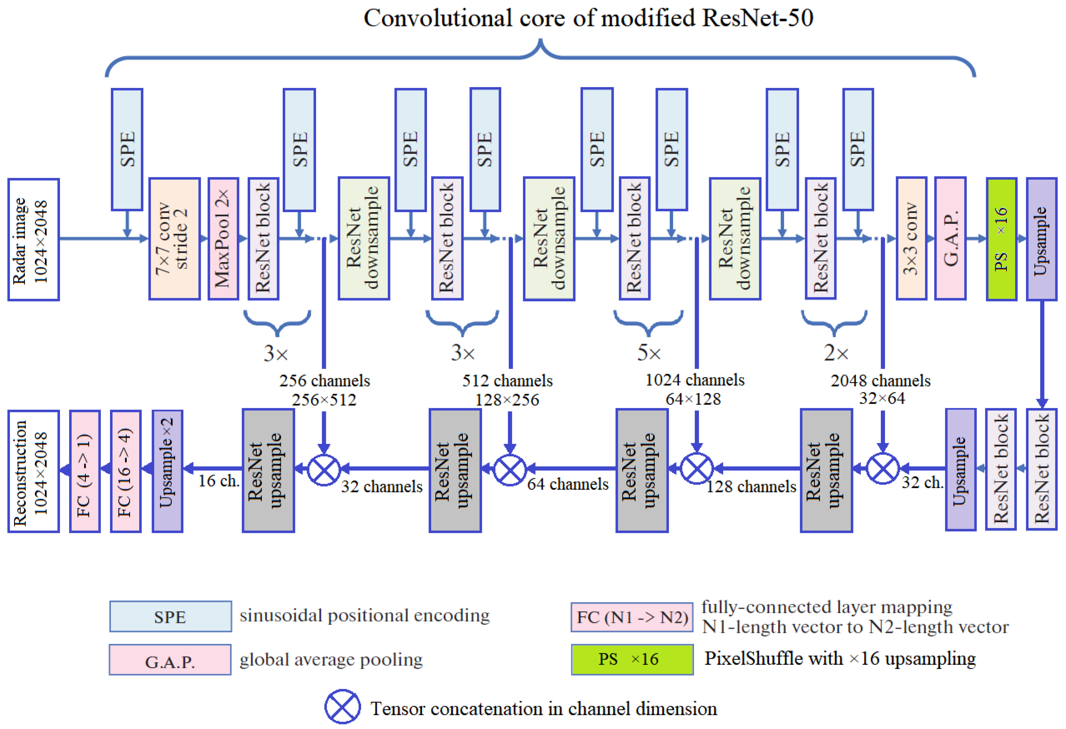
Figure 10.
High-level architecture of the regression CNN model based on modified ResNet50 and feature aggregation.
Figure 10.
High-level architecture of the regression CNN model based on modified ResNet50 and feature aggregation.
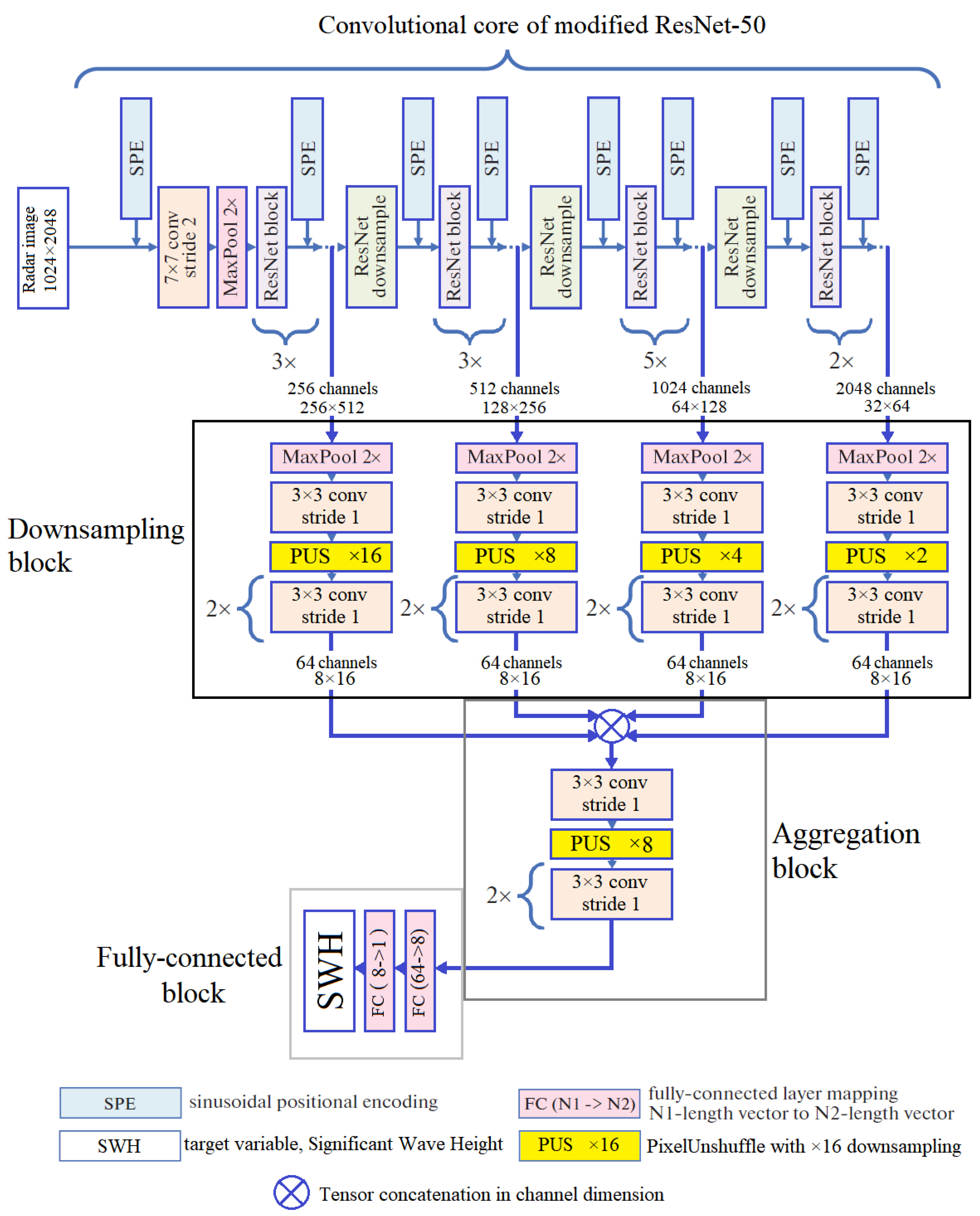
Figure 11.
Learning rate schedule used while training the reconstruction model.
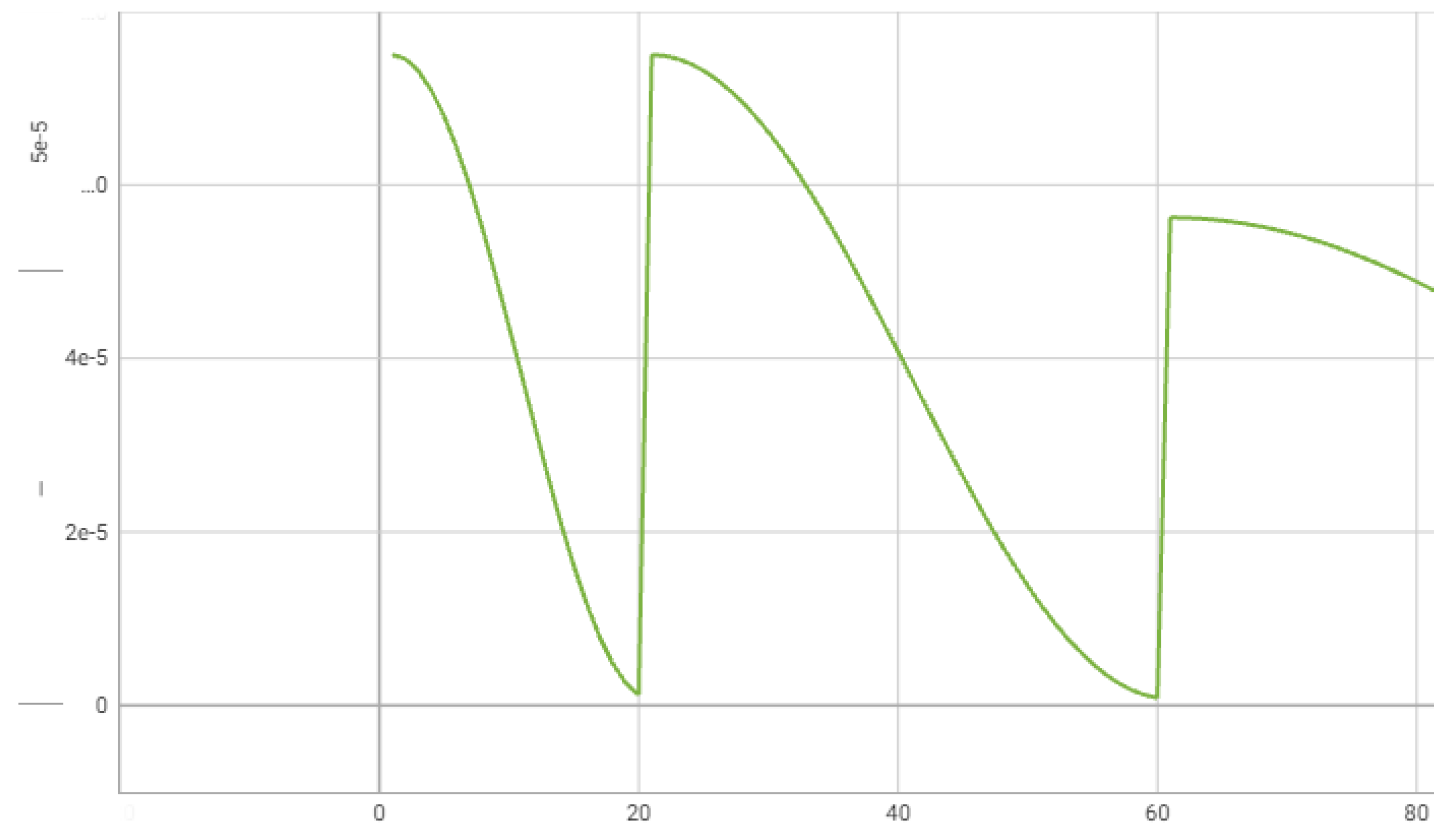
Figure 12.
Learning rate schedule used while training the reconstruction model on step Two: (a) stage ; (b) stage .
Figure 12.
Learning rate schedule used while training the reconstruction model on step Two: (a) stage ; (b) stage .
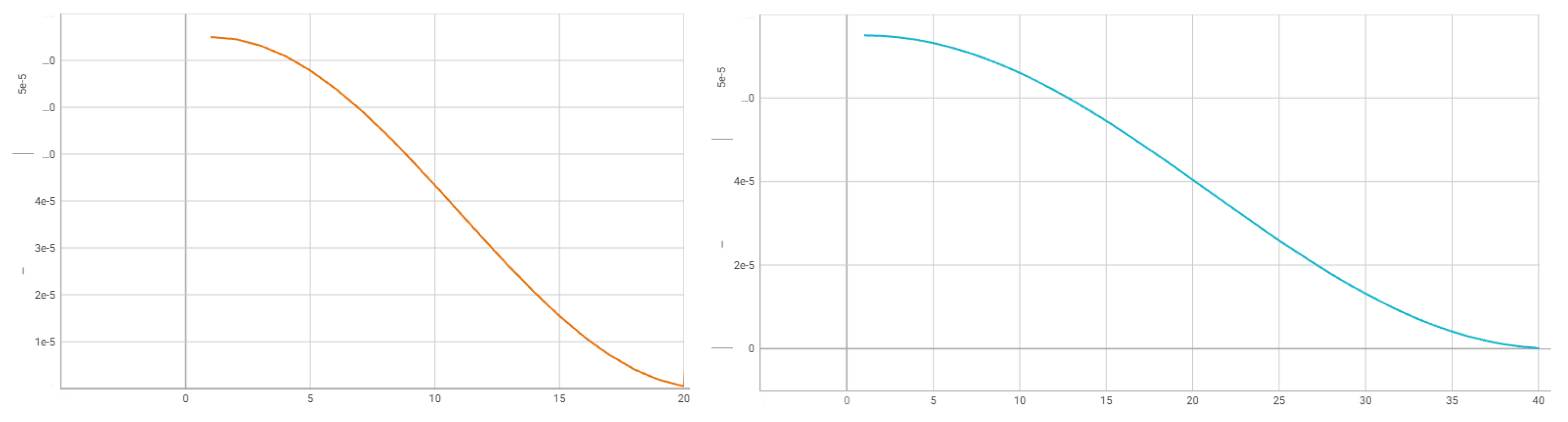
Figure 13.
Learning rate schedule used while training the reconstruction model on step Three: (a) stage ; (b) stage ; (c) stage .
Figure 13.
Learning rate schedule used while training the reconstruction model on step Three: (a) stage ; (b) stage ; (c) stage .
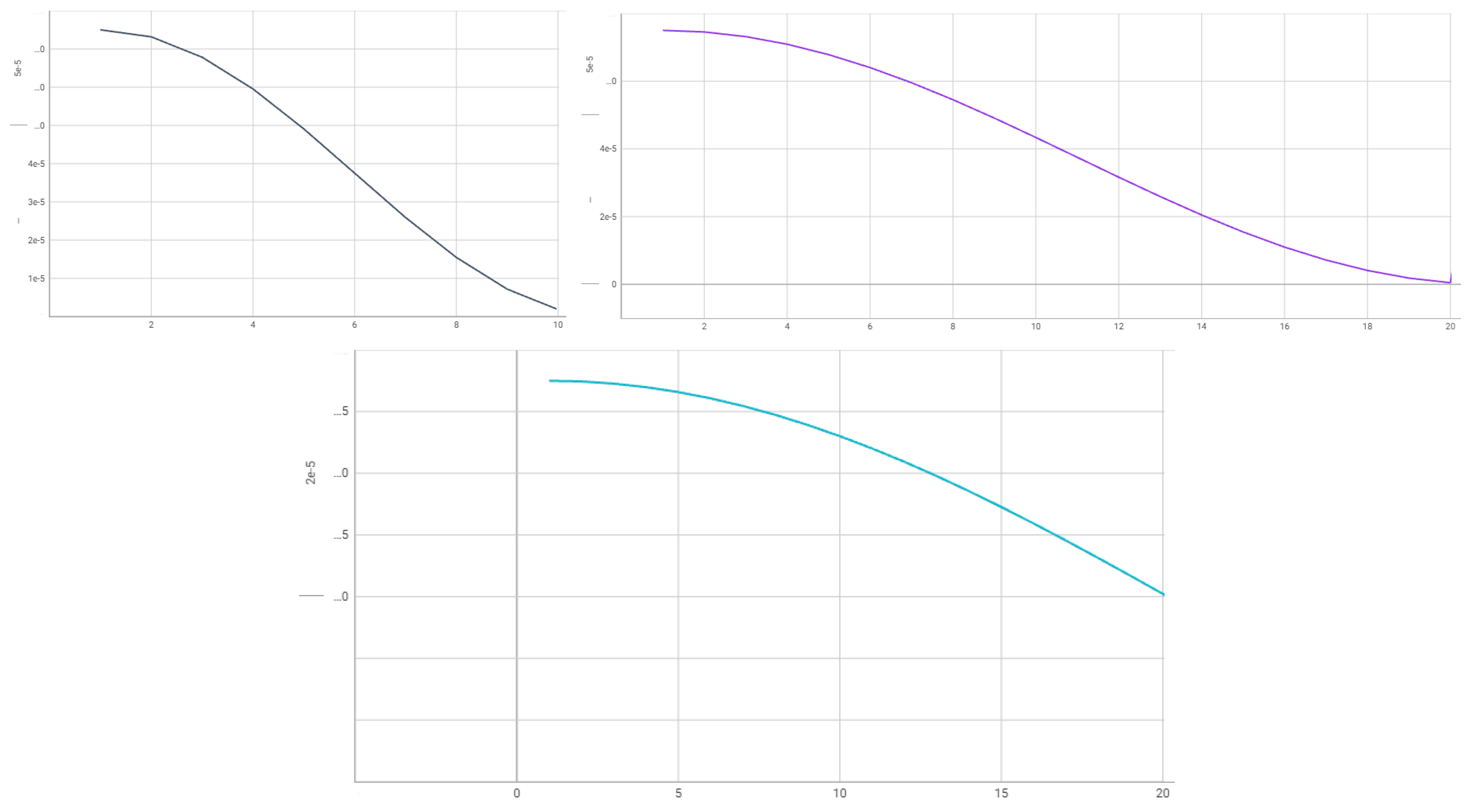

Table 1.
Research expeditions.
| Expedition | Departure | Arrival | No. of Spotter buoy locations | No. of SeaVision locations |
|---|---|---|---|---|
| ASV50 | Kaliningrad, Russia, 7 Aug 2020 | Arkhangelsk, Russia, 13 Sep 2020 | 24 | 157 |
| AI57 | Kaliningrad, Russia, 25 Jun 2021 | Arkhangelsk, Russia, 21 Jul 2021 | 12 | 76 |
| AI58 | Kaliningrad, Russia, 10 Aug 2021 | Kaliningrad, Russia, 9 Sep 2021 | 16 | 55 |
| AI63 | Arkhangelsk, Russia, 29 Sep 2022 | Arkhangelsk, Russia, 7 Dec 2022 | 30 | 209 |
| Total | 82 | 497 |
Disclaimer/Publisher’s Note: The statements, opinions and data contained in all publications are solely those of the individual author(s) and contributor(s) and not of MDPI and/or the editor(s). MDPI and/or the editor(s) disclaim responsibility for any injury to people or property resulting from any ideas, methods, instructions or products referred to in the content. |
© 2023 by the authors. Licensee MDPI, Basel, Switzerland. This article is an open access article distributed under the terms and conditions of the Creative Commons Attribution (CC BY) license (http://creativecommons.org/licenses/by/4.0/).
Copyright: This open access article is published under a Creative Commons CC BY 4.0 license, which permit the free download, distribution, and reuse, provided that the author and preprint are cited in any reuse.


