Application of the Polynomial Chaos Expansion to the Uncertainty Propagation in Fault Transients in Nuclear Fusion Reactors: DTT TF fast current discharge

Preprint

Article

Application of the Polynomial Chaos Expansion to the Uncertainty Propagation in Fault Transients in Nuclear Fusion Reactors: DTT TF fast current discharge

Altmetrics

Downloads

Views

Comments

A peer-reviewed article of this preprint also exists.

This version is not peer-reviewed

Submitted:

11 December 2023

Posted:

12 December 2023

You are already at the latest version

Alerts

Abstract

Nuclear fusion reactors are composed by several complex components whose behaviour may be not certain a priori. This uncertainty may have a significant importance in the evolution of fault transients in the machine, causing unexpected damages to its components. For this reason a suitable method for the uncertainty propagation during those transient is required. The Monte Carlo method would be the reference option, but it is, in most of the cases, not applicable due to the large amount of required simulations to be repeated. In this context the Polynomial Chaos Expansion has been considered as a valuable alternative. It allows to create a surrogate model of the original one in terms of orthogonal polynomials. Then, the uncertainty quantification is performed repeatedly calling this much simpler and faster model. Using the fast current discharge in the Divertor Tokamak Test Toroidal Field (DTT TF) coils as a reference scenario, this method has been applied: the uncertainty on the parameters of the Fast Discharge Unit (FDU) varistor disks is propagated to the simulated electrical and electro-magnetic relevant effects. Eventually two worst case scenarios have been analyzed from the thermal-hydraulic point of view with the 4C code, simulating a fast current discharge as a consequence of a coil quench. Eventually it has been demonstrated that the uncertainty on the inputs (varistor parameters) strongly propagates obtaining a wide range of possible scenarios in case of accidental transients. This result underlines the necessity to take into account and propagate all possible uncertainties in the design of a fusion reactor, according to the Best Estimate Plus Uncertainty approach.

Keywords:

Subject: Engineering - Energy and Fuel Technology

1. Introduction

Nuclear facilities, like fission reactors and, in the future, fusion reactors, are extremely complex systems both from the physical and technological point of view. For example, in fusion reactors, many components are first-of-a-kind. The widespread of fusion reactors in the future will be possible if these technologies will reach the maturity in terms of industrial production. At the same time, the construction of the first fusion reactors will help to achieve this maturity. However, currently the behaviour of these components is characterized by intrinsic uncertainties. When simulating a transient, the latter propagate from the single components to the overall system behavior, possibly leading to foresee serious damages to the reactor. For this reason it is relevant to estimate the impact of the uncertainty of the data used as inputs to the model on the final results of the simulations, already from the design phase. This will allow to set proper thresholds to the uncertainties requested to the supplier of the different components, to avoid damages to the reactor. The reference option for the non-intrusive (i.e. not requiring modifications of the model) uncertainty propagation (UP) analysis is the Monte Carlo (MC) method. This approach is based on the definition and the random sampling of a set of uncertain inputs, then deterministic calculations with these inputs are performed and the final results can be aggregated to obtain statistical information about the output.

However, the use of this method is often not feasible due to the very large amount of simulations required to reach the convergence, in view of the computational time required to perform each single simulation with complex high-fidelity codes. To face this problem several different methods have been proposed in the literature. An option is to reduce the number of simulations for the error quantification approximating the input distribution rather than the model, like in the Unscented Transform (UT) technique [1,2]. Another possibility is to build a surrogate model and use it instead of the real model to perform the uncertainty quantification, like in the Gaussian process modeling [3] and the Polynomial Chaos Expansion (PCE) [4,5]. The main advantage of this alternative is that the surrogate model is orders of magnitude faster than the corresponding real model.

The PCE has been employed in this work, using the python module chaospy [6], to analyze the uncertainty propagation during a Fast current Discharge (FD) in the Divertor Tokamak Test (DTT) facility Torioidal Field (TF) magnet system.

The uncertainty is given by the parameters of the characteristic of the Fast Discharge Unit (FDU) varistor, influencing the evolution of the coil current during FD. This causes both electrical (e.g. modification of coil peak voltage, variation of deposited energy in the FDU, etc.) and electro-magnetic (EM) drawbacks. Indeed, varying the evolution of the coil currents means varying the magnetic field time derivative which translate into a modification of the eddy currents induced within the TF coil casing, and, as consequence, a modification of the Joule power deposited. In this work, the uncertainties on the above mentioned results have been assessed using PCE. The electrical results have been obtained by an object oriented model developed using the Modelica language in the open source environment OpenModelica [7]. The uncertainty obtained with PCE has been benchmarked against the MC method, since computational time was still reasonable. On the other hand the EM results have been computed with 3D-FOX [8]. In this case the benchmark of the PCE outcomes with those of MC was impossible due to the excessive computational time required by the EM simulations. For this reason a benchmark of the results obtained with PCE against the UT method is proposed.

Eventually, from the statistical distribution of EM results two worst case scenarios have been identified and used as input to the thermal-hydraulic (TH) model, developed with the 4C code [9]. A fast discharge triggered by a quench initiated at the minimum temperature margin location in the coil has been analyzed. These analyses allowed to demonstrate that the uncertainty on the input data (varistor parameters) will lead to a wide range of possible accidental transients which must be carefully considered not to overlook some scenario pontentially dangerous for the machine integrity.

2. Methodology

The analysis of the TF FD transient described in this work can be divided in three consecutive sub-blocks related to the three pieces of physics considered in the analysis:

Electrical (EL) simulation of the magnet power supply system;
Electro-Magnetic (EM) modeling of the TF coil casing to evaluate the Joule power generated by eddy currents induced in it during the transient;
Thermal-hydraulic (TH) analysis of the magnet to assess the effect of the Joule power deposition in the casing and AC losses in the superconducting (SC) cables on the coil performance.

The logical connections between the three physics analyzed in the sub-blocks, as well as their main outcomes are schematically represented in Figure 1.

2.1. Electrical model

The power supply circuit of the DTT TF coils and its FDUs have been simulated by means of an object oriented model developed in OpenModelica [10]. The structure of the electrical circuit is taken from [11]: the eighteen TF coils are splitted in three groups of six coils each, connected in series; and the three groups are in turn connected in series among them and with the three FDUs, alternating one FDU and one group of coils. Each TF coil is modelled considering the self inductance and the mutual inductances of the other TF coils, based on the inductance matrix of the DTT TF system [12], solving the following equation:

Δ V_{i} = \sum_{j = 1}^{N} L_{i, j} \cdot \frac{d I_{j}}{d t} i \in [1, N],

(1)

where L is the inductance matrix and N is the number of TF coils in the tokamak (18 in DTT). The inductance matrix L is square and has the coils self inductances on the main diagonal and the mutual inductances out of the main diagonal.

The FDU is modelled as the parallel of the dumper and an ideal switch normally closed; when the fast discharge is triggered, the switch is opened forcing the current to flow through the dumper. In the meanwhile the power supply, modelled as an ideal current generator (forcing the nominal current of

42.5

kA in DTT [13]) taken from the Modelica Standard Library [7], is disconnected from the circuit so that the current in the loop decreases. The FDU dumper is composed of a collection of varistor disks [12], modelled here as an equivalent single disk whose characteristic is described by the following equation.

Δ V = K \cdot I^{β} .

(2)

The two parameters describing the varistor behaviour (K and

β

) are affected by epistemic uncertainty (i.e. there is a lack of knowledge of their values due to fabrication processes). Indeed, they can be assumed as uniformly distributed in the following ranges:

K \in [8.134, 13.05],

(3)

β \in [0.562, 0.595]

(4)

and have been considered here as statistically independent. When trying to numerically predict the behavior of the TF coil system during a FD, the uncertainty of these parameters is then propagated through the analysis of all the model sub-blocks, requiring an uncertainty propagation analysis.

2.2. Electro-Magnetic model

The EM model for the evaluation of the eddy currents induced in the coil casing during the FD is developed within the 3D-FOX, a finite element electromagnetic code developed at Politecnico di Torino [8]. The model solves Faraday’s and Ampère’s laws using the A-formulation. The eddy currents distribution is then used to evaluate the power distribution in the TF coil casing by means of the Ohm’s law. The Joule power deposition is suitably averaged before providing it as input to the TH model, as explained in [8].

The simulation setup is the same presented in [8], adding cyclic periodic boundary conditions to the model of a single TF coil to exploit the periodicity of the tokamak to simulate the effect of the simultaneous discharge of all the TF coils.

2.3. Thermal-hydraulic model

The model of the DTT TF coils developed within the 4C code [9], presented in [14] and used for the simulation of several transients, is adopted for the TH analysis. The TH simulation setup are taken from [15], while the logical connection between the EM module (3D-FOX) and the TH one (4C code) is reported in detail in [8].

2.4. Uncertainty propagation analysis

One of the aims of the uncertainty propagation is to evaluate the impact of the uncertainties of the inputs on the outputs of a generic model and to asses how they affect the performance of the system represented by the computational model. Usually, UP is a demanding activity requiring a large amount of expensive simulations. At the same time, UP is mandatory since uncertainties can have a dramatic impact on the performance of nuclear systems. In fact, one of the most recent methodologies for the licensing of nuclear system is the so called Best Estimate Plus Uncertainty method [16,17], where the output is provided together with its uncertainty. This approach is progressively substituting the more traditional conservative approach.

To reduce the computational burden of the UQ, several methods have been proposed in the literature. In this work, the Polynomial Chaos Expansion has been used, together with the Unscented Transform for verification purposes, benchmarking the two methods. Only in the case of the EL model, the Monte Carlo approach has also been used as a further reference benchmark, thanks to the sufficiently short computational time of the detailed model.

2.4.1. Polynomial Chaos Expansion

The Polynomial Chaos Expansion approximates a stochastic model

M (X)

, where the stochastic nature comes from the uncertainty of the inputs

(X)

, through a series of orthogonal polynomials. The random vector

X

is represented by a joint probability distribution which, in the case of independent variables (as in this work), is simply the product of the single marginal probability density functions associated with each input. It is possible to express the model

M

in terms of an expansion of orthogonal polynomials

Ψ

selected according to the joint distribution of the input:

M (X) = \sum_{c = 0}^{\infty} a_{c} Ψ_{c} (X) \approx \sum_{c = 0}^{C} a_{c} Ψ_{c} (X),

(5)

where

a_{c}

are the coefficients of the multivariate orthogonal polynomials. The infinite sum in Equation (5) must be truncated at the first C terms due to practical reasons. The total number of terms C in the polynomial expansion depends on the polynomial order p and on the dimension of the input d and, according to the total degree truncation scheme, it is:

C = \frac{(p + d)!}{p! d!} .

(6)

There are several techniques for the evaluation of the polynomial coefficients, which are the unknowns of the PCE method. Some of these techniques are intrusive, requiring the modification of the model equations (e.g. stochastic Galerkin method [18]), others are non-intrusive, where the computational model is treated as a black-box (e.g. pseudo-spectral projection, point collocation [19] and stochastic testing [20]). In this work, the pseudo-spectral projection method implemented in chaospy has been used.

In the pseudo-spectral projection method, the coefficient of Equation (5) are computed through a quadrature integration scheme as:

a_{c} = \int_{- \infty}^{+ \infty} d X M (X) Ψ_{c} (X) w (X) \approx \sum_{i = 1}^{I} M (X_{i}) Ψ_{c} (X_{i}) w (X_{i});

(7)

where

X = X_{1}, X_{2}, . . ., X_{I}

is the vector of quadrature nodes generated according to the chosen quadrature rule,

w (X_{i})

are the corresponding weights and

M (X_{i})

are the exact model evaluations at node

X_{i}

. Thus, knowing the values of

M (X_{i})

for all the nodes and the appropriate expansion of orthogonal polynomials, it is possible to compute the coefficients

a_{c}

and a surrogate model of

M (X)

according to Equation (5). Hermite and Legendre polynomials are typically used as orthogonal polynomials for Gaussian and uniform distributions, respectively; see [5] for a more detailed description about the relation between the type of distribution and the most appropriate orthogonal polynomial set. Once the Is exact model simulations have been performed, the polynomial metamodel can be used to evaluate the first moments of the output distributions (i.e. mean and variance), but also the complete distributions and other quantities like Sobol’ sensitivity indices, which allow to rank the input parameters based on how much they affect the uncertainty of the output.

In principle, the surrogate model is able to reproduce the results of the exact model inside the range of validity of the input distributions, with the advantage of being much faster and simpler. It is this peculiar characteristic which justifies the use of the metamodel for uncertainty quantification purposes.

2.4.2. Unscented Transform

The intuition upon which the Unscented Transform technique is based is that it is simpler to approximate the distribution of the inputs rather than approximate the model used to generate the output distribution. The approximation of the input distribution is obtained generating a set of sigma points that represent the probability distribution of the input and which are used to feed the exact model. According to the literature [21], 2d+1 sigma points are sufficient to get a good representation of the input and of the mean and variance of the output, where d represents the dimension of the input perturbed data. The UT generally requires less simulations than the PCE, but it gives a limited amount of information (namely the first two moments of the output distribution), assuming a Gaussian distribution for the output. However, in some cases, it could be sufficient to know the mean and the variance of an output distribution, making the UT an interesting technique for preliminary evaluations.

Among the several algorithms presented in literature, here the so called Generalized Unscented Transformation [22] has been employed, since it allows to deal with constrained sigma points like those generated starting from the uniform distributions in Equation (3) and Equation (4) for the DTT FDU input parameters at hand, avoiding to have non-physical sigma points outside of the prescribed distributions.

In this work, the UT has been employed to check that at least the first two moments calculated with the PCE are correct, to add an additional benchmark also in the EM model in which the comparison to the MC was not viable due to excessive computational time of the detailed model.

3. Results

In this section the results of the three modules are summarized, including the statistical analysis of the uncertainty propagation, from the inputs to the outputs of both EL and EM models. The generation ans simulation of a TH worst case scenario, selected according to the uncertainty quantification analysis, is also presented.

3.1. Results of the Electrical model

The EL model is sufficiently fast to allow the analysis of its uncertainty propagation on the results by a Monte Carlo approach. For this reason a MC analysis has been developed exploiting the interoperability of Python and Modelica assured by OMPython [7] and DyMat packages. The MC method simply consists of sampling a large number N of random points from the input distribution and performing a simulation for each of these points giving a result

ξ_{i}

. In the MC algorithm the average results

\bar{ξ_{N}}

are computed as:

\bar{ξ_{N}} = \sum_{i = 1}^{N} \frac{ξ_{i}}{N} .

(8)

Together with the average value both standard deviation (STD) and relative standard deviation (RSD) are computed, according to the following equations:

S T D (ξ_{N}) = \sqrt{\frac{1}{N} \sum_{i = 1}^{N} {(ξ_{i} - \bar{ξ_{N}})}^{2}},

(9)

R S D (ξ_{N}) = \frac{S T D (ξ_{N})}{\bar{ξ_{N}} \cdot \sqrt{N}} .

(10)

The RSD is used as indicator to stop the sampling of random points once the required tolerance is reached. In this case, the required tollerance for the RSD was

0.1 %

, and was reached after

\approx 28500

simulations. The Equation (10) underlines one of the main drawbacks of MC, namely its slow convergence (as

1 / \sqrt{N}

), asking for a large number of simulations.

The statistical distributions of the following four relevant results have been obtained from the MC run and are reported in Figure 2:

$τ \to$ time required for the current to decrease from nominal value to $0.1 A$ ;
$I^{2} \cdot t = \int_{0}^{t} I^{2} (t^{'}) d t^{'}$ , considering its asymptotic value, which is proportional to the energy extracted from the TF coils during the FD;
$Δ V_{F D U} \to$ peak voltage on the FDU during the discharge;
$Δ V_{T F} \to$ peak voltage on the TF coil during the discharge.

The resulting mean values of the monitored variables and their standard deviations are reported in Table 1.

The same model has been analyzed using the PCE to reduce the required number of simulations to obtain the same statistical information. Quadrature and polynomial orders from 1 to 3 have been tested and the results have been compared to those of the MC method, obtaining extremely good agreement for all the monitored variables using order 3, as it is shown in Figure 3. Indeed the norm 2 of the relative difference between the MC and PCE order 3 distribution results in a maximum discrepancy of 0.05 % between the two.

This allows performing only sixteen simulation of the detailed model as training set. In fact, in the case of the pseudo-spectral projection method, the number of simulations required is given by

{(p + 1)}^{d}

, where p is the polynomial degree at which the truncation occurs (3 in this case) and d the dimension of the input space (2 in the case at hand). This choice results in a polynomial with 10

a_{c}

coefficients, according to Equation (6). Here, the quadrature nodes and the weights have been obtained using the Gaussian quadrature rule.

To better highlight the accuracy of the PCE results the comparison between the mean values and their standard deviation obtained with MC and PCE is reported in Table 1. Using the PCE it has been possible to evaluate also the current and

I^{2} \cdot t

evolution. Knowing the statistical distribution of each point in the evolution, it has been possible to evaluate an average evolution and a

1 - 99 %

confidence interval, for both variables, reported in Figure 4.

Eventually, the UT method has been applied as well. In the framework of the EL model its application is not particularly relevant since the reduction of the required number of simulation is limited (five simulation instead of sixteen) and the amount of statistical information is limited to the average and the standard deviation, without providing effective information on the distribution. However this method has been introduced as a useful benchmark for the EM model in which the MC method can not be applied due to the excessive computational cost.

The five UT sigma points have been generated according to the Generalized Unscented Transformation algorithm and the results are summarized in Table 1, showing very good agreement between the three methods. Indeed, the maximum relative error on the computed mean values is ≈ 0.06 % (smaller than the tolerance imposed to check the convergence of the MC run), while the maximum relative error on the computed variance is ≈ 0.6 %.

The results show a non-negligible variance, justifying the necessity to further propagate the uncertainties through the EM model. In particular, as the relative standard deviation on the outputs of the EL model, computed as

σ / \bar{V}

is generally larger than that on the input distributions in Equation (4) and Equation (3), the electrical model seems to amplify the uncertainties.

3.2. Results of the Electro-Magnetic model

The MC method was not applicable to the uncertainty propagation analysis in the EM model due to the increase of the computational time

(\approx 1 d a y / s i m u l a t i o n)

of the detailed model. For this reason the PCE of quadrature order 3 has been used to build a surrogate model of the detailed one, based on its results, since it proved to be accurate to replace the detailed EL model too. The 3D-FOX calculates the evolution of the power

P (t)

deposited in the TF coil casing. The monitoring variables have been extracted from this evolution, considering:

The peak of the deposited power $P_{p e a k}$ ;
The overall deposited energy $E = \int_{0}^{t_{e n d}} P (t) d t$ .

The statistical distributions of the peak of the deposited power and of the energy deposited are reported in Figure 5: they highlight how the uncertainty on the inputs translates into a huge uncertainty on the peak power and deposited energy. Neglecting this uncertainty propagation may lead to disregard the worst case scenarios connected to this transient, concerning e.g. its TH effects.

The average value and the standard deviation of the peak of the deposited power and of the deposited energy computed with the PCE have been benchmarked against those evaluated with the UT. The comparison of the results is shown in Table 2.

The benchmark shows an excellent agreement between the PCE and the UT. This does not guarantee the accuracy of the statistical distribution obtained with PCE, but suggests that the metamodel developed reproduces properly the main statistical data, namely the mean and the variance.

As already done for the evolution of the current and of

I^{2} \cdot t

in the EL model analysis, here the average power evolution and its

1 - 99 %

confidence range have been calculated using the PCE and are shown in Figure 6.

The width of the

1 - 99 %

confidence range highlights the importance of considering the uncertainty on the input data to evaluate the worst case scenario to be retained for the analysis of this transient. Moreover, the impact of the uncertainty is much larger in the first part of the transient (peak region). This is expected since the first part of the transient is driven by the large value of the time derivative of the current at the beginning of the FD, strongly affected by the K and

β

parameters of the varistors. On the contrary, the last part of the transient is less affected by the uncertainty of the inputs, as the time derivative of the current is reduced, reducing consequently the power deposited.

A further benchmark of the metamodel based on PCE is performed applying it to the inputs represented by the sigma points generated for the UT computations and comparing the results to those obtained in those points with the detailed EM model (3D-FOX). To ensure a fair benchmark, the UT sigma points used do not belong to the PCE model training set.

The comparison is shown in Table 3 including the relative error

ε_{V}

on variable V obtained as:

ε_{V} = \frac{V_{P C E} - V_{3 D - F O X}}{V_{3 D - F O X}} .

(11)

The larger relative discrepancy is smaller than

0.5 %

, which is considered a satisfactory accuracy. This benchmark does not guarantee the level of accuracy for the entire parameter space

(K, β)

, but demonstrates that the model is able to reproduce properly the detailed model results in the entire parameter space, covered by the UT sigma points. In fact, by definition, the sigma points are constructed by the UT algorithm to cover in the best possible way the input space, with the smallest number of points.

3.3. Identification of the worst case scenarios

The relevant worst case scenarios (WCSs) to be used as input to the TH model must now be identified. In the WCS selection both EL and EM aspects must be considered. Indeed, a fast current discharge is fundamental to promptly protect the magnet from the quench, but at the same time deposits a lot of energy in the coil casing, contributing to the coil temperature increase. For this reason it is relevant to evaluate the

(K, β)

couples which cause the slowest discharge (WCS1) and that lead to the highest energy deposition in the coil casing (WCS2), and perform their TH analysis. The two scenarios are clearly distinct, as the slower is the discharge, the smaller is the energy deposited in the casing (driven by the time derivative of the current). Thus they will be generated by points standing at the opposite boundaries of the

(K, β)

plane. This statement is confirmed by Figure 7 in which the

τ

and deposited energy values have been mapped, using the PCE model, on the

(K, β)

plane. The specific values of K and

β

generating the two WCSs are (

K = 8.134

β = 0.562

) for WCS1 and (

K = 13.05

β = 0.595

) for WCS2.

Using these values of K and

β

, the inputs to the TH model have been computed.

The first required input is the evolution of the coil current, evaluated with the EL model and it is reported in Figure 8(a). As expected, the two evolutions are very different and this will strongly influence the quench evolution.

The second required input is the power deposited in the casing, including both its evolution and distribution (to account for its non-uniformity). The PCE metamodel has been trained on a set of 3D-FOX simulations considering the evolution of the overall power deposition, to reduce the computational cost. Therefore, a dedicated run of the 3D-FOX has been performed for each of the two selected WCSs to prepare the detailed input to the 4C code, namely the spatial discretization of the power deposition in the casing [8]. The total power deposited in one TF coil casing in the two WCSs is reported in Figure 8(b), confirming that the fastest discharge is actually responsible of the larger energy deposition.

3.4. Results of the Thermal-Hydraulic model

The inputs have been adopted to simulate a FD triggered by the magnet quench. In the simulation the quench has been obtained by a local heat deposition at the location where the minimum temperature margin is computed in nominal operation, i.e. in the first turn of the two central pancakes at inboard equator. In this work, 50 kW/m of external power (e.g. a very concentrated beam of particles coming from the plasma) have been deposited in 10 cm of SC cable around the minimum margin location of pancake 6 for 0.1 s. The power deposition erodes the temperature margin leading the magnet to quench initiation and propagation. The FD is triggered by the quench detection system when the voltage computed across the coil overcomes the 100 mV threshold, waiting then for a validation time of 1.5 s [23] to reduce the spurious detections.

The evolution of the voltage computed with the 4C code in the two WCSs is reported in Figure 9. The WCS2, characterized by a faster discharge, leads to a faster response to quench protection, reducing the quench propagation (and therefore the voltage buildup) in the Winding Pack (WP). Due to the inter-pancake thermal coupling, the neighbouring pancakes (namely, 5 and 7) are also heated up, possibly quenching. However, the voltage raise in pancakes 5 and 7 is almost negligible in WCS2 due to the faster reduction of the current; on the contrary, in WCS1 the delayed current decrease causes a quench initiation and propagation also in those pancakes. Quench initiation in pancake 7 is slightly delayed with respect to pancake 5 due to the smaller magnetic field there, being if further away from the coil center.

The two scenarios also differ in term of the hot-spot (HS) temperature, that may lead to permanent damages to the coil. Indeed, as shown in Figure 10 where the HS temperature reached during the transient is plotted for each pancake, the hot spot temperature is larger, in the central pancakes, in the WCS1, featuring a larger Joule power deposition. Opposite trend is observed in side pancakes (e.g. pancake 1) in which the quench is not initiated and the heating is due to the thermal contact with the casing, where eddy current power is deposited. Given that the power deposition in the casing is larger in WCS2 (see Figure 8(b)) also the power transferred from the casing to the WP is larger and thus the conductor temperature increases more. From the bar plot in Figure 10 it is also possible to appreciate the effect of the inter-pancake heat diffusion, visible from the progressive temperature decrease moving far away from the quenched (central) pancakes.

The importance of reducing the current in the fastest possible way is clear comparing the hot spot temperature in the two scenarios. Indeed, HS temperature is much larger in WCS1, due to the faster current decrease in WCS2. On the contrary, the temperature increase in the side pancakes, given by the eddy current power deposition in the casing, is similar in the two cases, despite the consistent difference in the casing power deposition between them, as can be seen from Figure 8(b). Actually, the timescale of the heat transfer from the casing to the WP is quite slow if compared to the current discharge duration, also in the slower WCS1.

These results show that the uncertainty on the characteristic parameters of the varistors leads, eventually, to a wide range of quench evolutions. Increasing as much as possible the precision on the varistor parameters during their manufacturing is fundamental to have reliable predictions and therefore a safe reactor operation. Moreover, the preferable direction in the refinement of the varistor characteristics is that leading to faster current discharges; this, despite the larger power deposition in the coil casing due to eddy currents, ensures a faster response to the quench and thus limits its propagation, reducing the HS temperature and therefore the risk to damage the coil.

4. Conclusions and perspective

In this paper, the Polynomial Chaos Expansion has been adopted to assess the uncertainty propagation in a transient relevant for the safe operation of a nuclear fusion plant. The uncertainty in the characteristic parameters of the varistors of the fast discharge units of the DTT TF coils have been propagated to the computed results during a fast discharge transient. The uncertainty has an impact on the actual current evolution during the discharge which influences both the eddy currents induced in the coil casing and the TH behaviour of the coil during the quench propagation.

The current evolution during the discharge has been computed, as a function of the varistor parameters, with an object oriented electrical model developed using the Modelica language. The uncertainty propagation from the varistor parameters to the effective current evolution has been assessed using a surrogate model based on the PCE, which has been successfully benchmarked against the Monte Carlo approach. The obtained statistical distribution of the current evolution has been used as input to the electro-magnetic model developed using the 3D-FOX tool to computing, again with a PCE surrogate model, the statistical distribution of the power (and energy) deposition in the coil casing due eddy currents.

Eventually, both these results (current and power evolution) have been used to identify two possible worst case scenarios to be simulated with the thermal-hydraulic model, developed with the 4C code. The two cases are the slowest current dump and the highest power deposition in the casing.

The comparison of the results of the thermal-hydraulic model shows that the considered uncertainty on the varistor parameters leads to a wide range of different results. For what concerns the quench protection, the reduction of the current discharge time, reducing the hot spot temperature, is preferable to the reduction of the power deposited in the casing due to eddy currents.

The effect of the latter is however important, especially on the hydraulic circuit pressurization and He venting. In perspective, more detailed models, including also the hydraulic circuits, will be used to assess this effect.

The application of the statistical methods also to the TH model will in future allow to identify other worst case scenarios between the two extreme ones analyzed in this work. Moreover, a reverse analysis will be performed with the aim of suggesting the maximum limits of uncertainty which are acceptable on the varistor parameters.

Author Contributions

Conceptualization, A.A. and M.D.B.; methodology, A.A. and M.D.B.;original draft preparation, A.A. and M.D.B.; supervision, R.B. and S.D; review and editing, R.B. and S.D. All authors have read and agreed to the published version of the manuscript.

Conflicts of Interest

The authors declare no conflict of interest.

References

Julier, S.J.; Uhlmann, J.K. New extension of the Kalman filter to nonlinear systems. Signal Processing, Sensor Fusion, and Target Recognition VI; Kadar, I., Ed. International Society for Optics and Photonics, SPIE, 1997, Vol. 3068, pp. 182 – 193. [CrossRef]
Julier, S.J. The scaled unscented transformation. Proceedings of the 2002 American Control Conference (IEEE Cat. No.CH37301), 2002, Vol. 6, pp. 4555–4559 vol.6. [CrossRef]
Rasmussen, C.E.; Williams, C.K.; others. Gaussian processes for machine learning; Vol. 1, Springer, 2006.
Wiener, N. The homogeneous chaos. American Journal of Mathematics 1938, 60, 897–936. [CrossRef]
Xiu, D.; Karniadakis, G.E. The Wiener–Askey polynomial chaos for stochastic differential equations. SIAM journal on scientific computing 2002, 24, 619–644. [CrossRef]
Feinberg, J.; Langtangen, H.P. Chaospy: An open source tool for designing methods of uncertainty quantification. Journal of Computational Science 2015, 11, 46–57. [CrossRef]
OpenModelica online documentation, 2023. Last accessed 27 June 2023.
Bonifetto, R.; De Bastiani, M.; Zanino, R.; Zappatore, A. 3D-FOX—A 3D Transient Electromagnetic Code for Eddy Currents Computation in Superconducting Magnet Structures: DTT TF Fast Current Discharge Analysis. IEEE Access 2022, 10, 129552–129563. [CrossRef]
Richard Savoldi, L.; Casella, F.; Fiori, B.; Zanino, R. The 4C code for the cryogenic circuit conductor and coil modeling in ITER. Cryogenics 2010, 50, 167–176. [CrossRef]
Fritzson, P.; Pop, A.; Abdelhak, K.; Ashgar, A.; Bachmann, B.; Braun, W.; Bouskela, D.; Braun, R.; Buffoni, L.; Casella, F.; Castro, R.; Franke, R.; Fritzson, D.; Gebremedhin, M.; Heuermann, A.; Lie, B.; Mengist, A.; Mikelsons, L.; Moudgalya, K.; Ochel, L.; Palanisamy, A.; Ruge, V.; Schamai, W.; Sjölund, M.; Thiele, B.; Tinnerholm, J.; Östlund, P. The OpenModelica Integrated Environment for Modeling, Simulation, and Model-Based Development. Modeling, Identification and Control 2020, 41, 241–295. [CrossRef]
Messina, G.; Lopes, C.R.; Zito, P.; Di Zenobio, A.; Zignani, C.F.; Lampasi, A.; Morici, L.; Ramogida, G.; Tomassetti, G.; Ala, G.; others. Transient Electrical Behavior of the TF Superconducting Coils of Divertor Tokamak Test Facility During a Fast Discharge. IEEE Transactions on Applied Superconductivity 2022, 32, 1–10. [CrossRef]
Lampasi, A. Private Comunication. 2023.
Zito, P.; Manganelli, M.; Lampasi, A.; Pipolo, S.; Lopes, R. Final design of the DTT Toroidal power supply circuit. Fusion Engineering and Design 2023, 192, 113595. [CrossRef]
Bonifetto, R.; Di Zenobio, A.; Muzzi, L.; Turtù, S.; Zanino, R.; Zappatore, A. Thermal-Hydraulic Analysis of the DTT Toroidal Field Magnets in DC Operation. IEEE Transactions on Applied Superconductivity 2020, 30, 1–5. [CrossRef]
Bonifetto, R.; De Bastiani, M.; Di Zenobio, A.; Muzzi, L.; Turtu, S.; Zanino, R.; Zappatore, A. Analysis of the thermal-hydraulic effects of a plasma disruption on the DTT TF magnets. IEEE Transactions on Applied Superconductivity 2022, 32, 1–7. [CrossRef]
Bucalossi, A.; Petruzzi, A.; Kristof, M.; D’Auria, F. Comparison between Best-Estimate–Plus–Uncertainty Methods and Conservative Tools for Nuclear Power Plant Licensing. Nuclear Technology 2010, 172, 29–47. [CrossRef]
D’Auria, F.; Camargo, C.; Mazzantini, O. The Best Estimate Plus Uncertainty (BEPU) approach in licensing of current nuclear reactors. Nuclear Engineering and Design 2012, 248, 317 – 328. [CrossRef]
Acharjee, S.; Zabaras, N. Uncertainty propagation in finite deformations––A spectral stochastic Lagrangian approach. Computer Methods in Applied Mechanics and Engineering 2006, 195, 2289–2312. [CrossRef]
Xiu, D. Fast numerical methods for stochastic computations: a review. Communications in computational physics 2009, 5, 242–272.
Zhang, Z.; El-Moselhy, T.A.; Elfadel, I.M.; Daniel, L. Stochastic Testing Method for Transistor-Level Uncertainty Quantification Based on Generalized Polynomial Chaos. IEEE Transactions on Computer-Aided Design of Integrated Circuits and Systems 2013, 32, 1533–1545. [CrossRef]
Julier, S.J.; Uhlmann, J.K. New extension of the Kalman filter to nonlinear systems. Signal Processing, Sensor Fusion, and Target Recognition VI; Kadar, I., Ed. International Society for Optics and Photonics, SPIE, 1997, Vol. 3068, pp. 182 – 193. [CrossRef]
Ebeigbe, D.; Berry, T.; Norton, M.M.; Whalen, A.J.; Simon, D.; Sauer, T.; Schiff, S.J. A Generalized Unscented Transformation for Probability Distributions, 2021, [arXiv:stat.ME/2104.01958].
Lopes, C.R.; Zito, P.; Lampasi, A.; Ala, G.; Zizzo, G.; Sanseverino, E.R. Conceptual Design and Modeling of Fast Discharge Unit for Quench Protection of Superconducting Toroidal Field Magnets of DTT. 2020 IEEE 20th Mediterranean Electrotechnical Conference ( MELECON), 2020, pp. 623–628. [CrossRef]

Figure 1. Logical connections between the three physics (and sub-blocks), and related results.

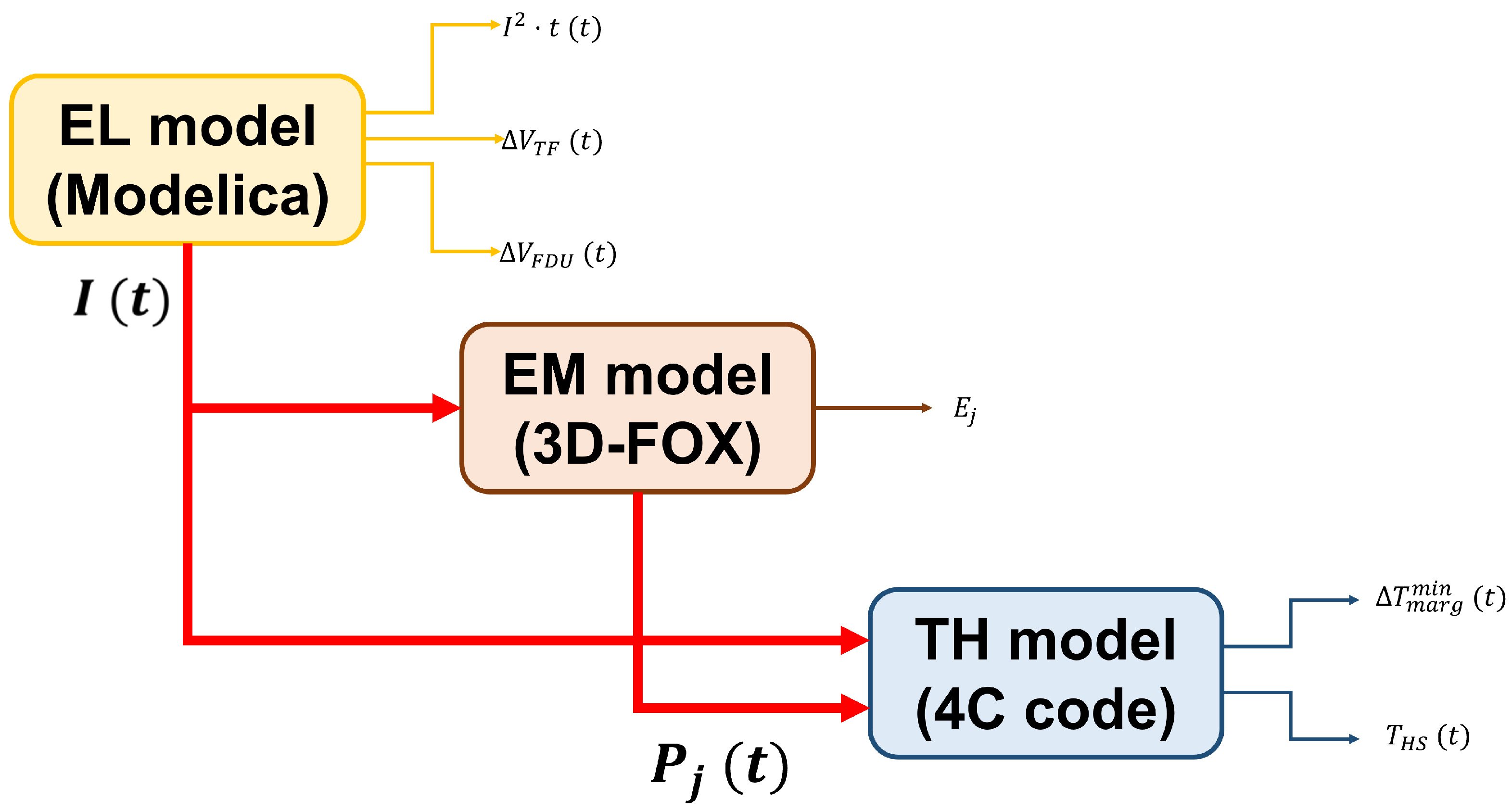
Figure 2. Statistical distribution of (a)

τ

, (b)

I^{2} \cdot t

, (c)

Δ V_{F D U}

and (d)

Δ V_{T F}

obtained with the MC method.

Figure 2. Statistical distribution of (a)

τ

, (b)

I^{2} \cdot t

, (c)

Δ V_{F D U}

and (d)

Δ V_{T F}

obtained with the MC method.

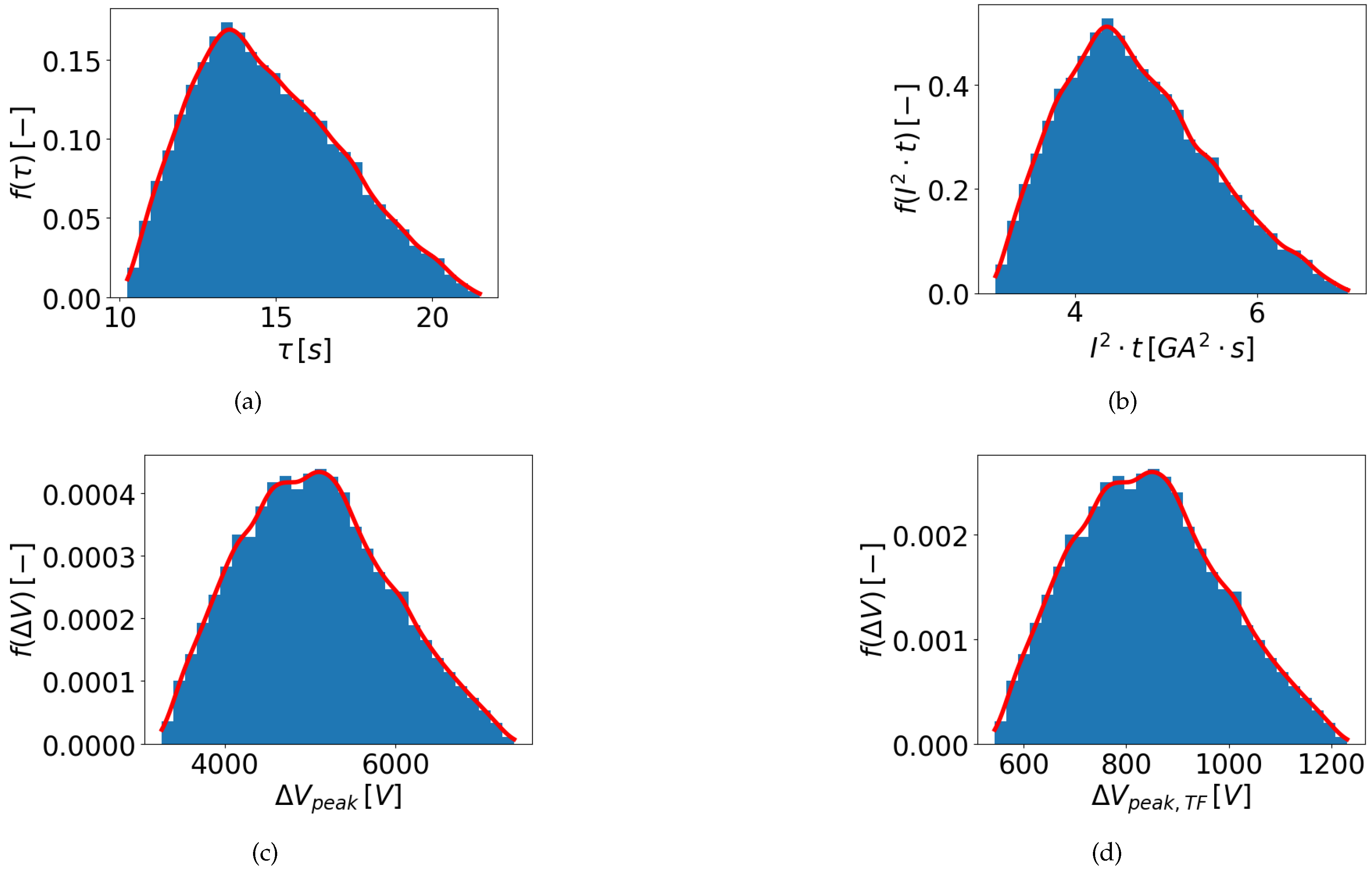
Figure 3. Statistical distribution of (a)

τ

, (b)

I^{2} \cdot t

, (c)

Δ V_{F D U}

and (d)

Δ V_{T F}

obtained with the PCE method. Comparison between performances of different PCE quadrature orders are shown for each distribution.

Figure 3. Statistical distribution of (a)

τ

, (b)

I^{2} \cdot t

, (c)

Δ V_{F D U}

and (d)

Δ V_{T F}

obtained with the PCE method. Comparison between performances of different PCE quadrature orders are shown for each distribution.

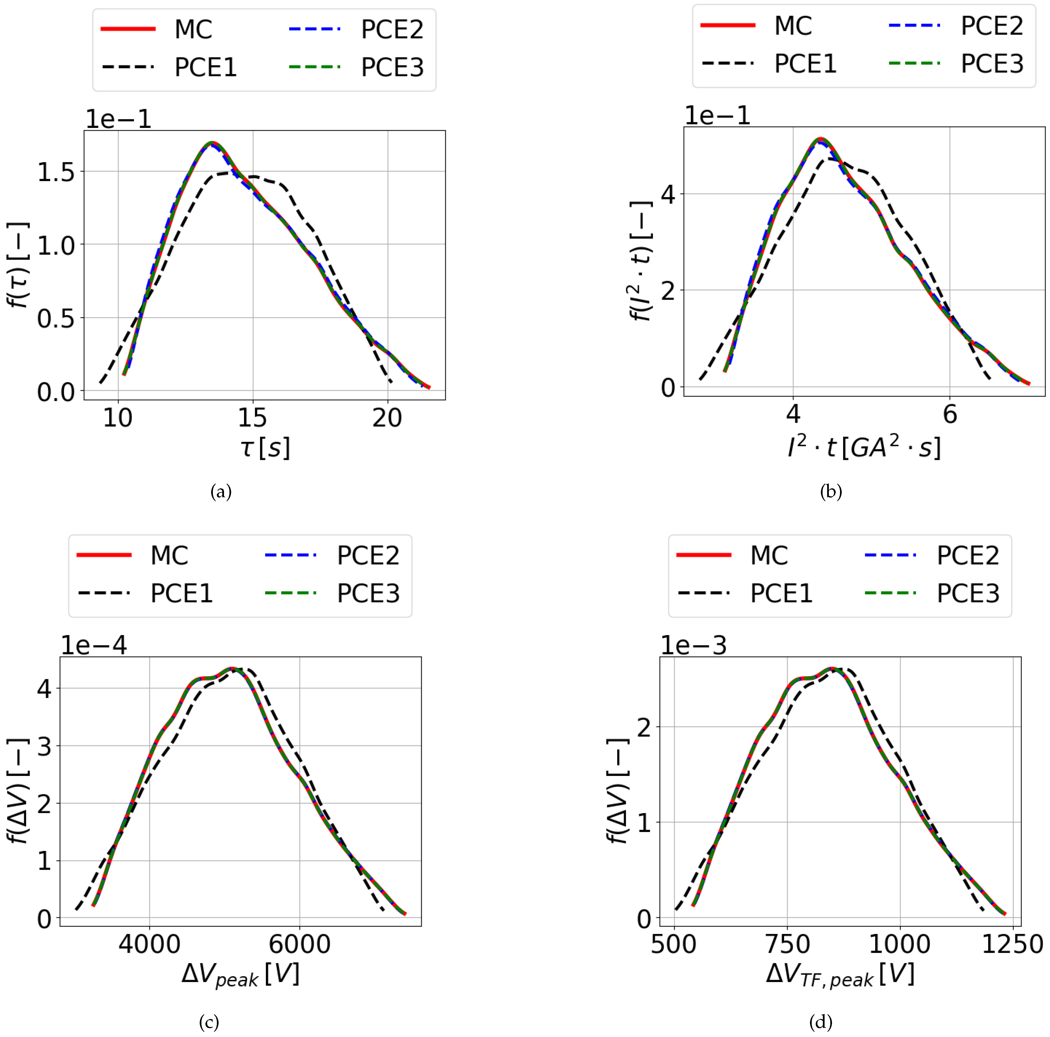
Figure 4. Average evolution of (a) current and (b)

I^{2} \cdot t

with respective

1 - 99 %

confidence range evaluated with PCE.

Figure 4. Average evolution of (a) current and (b)

I^{2} \cdot t

with respective

1 - 99 %

confidence range evaluated with PCE.

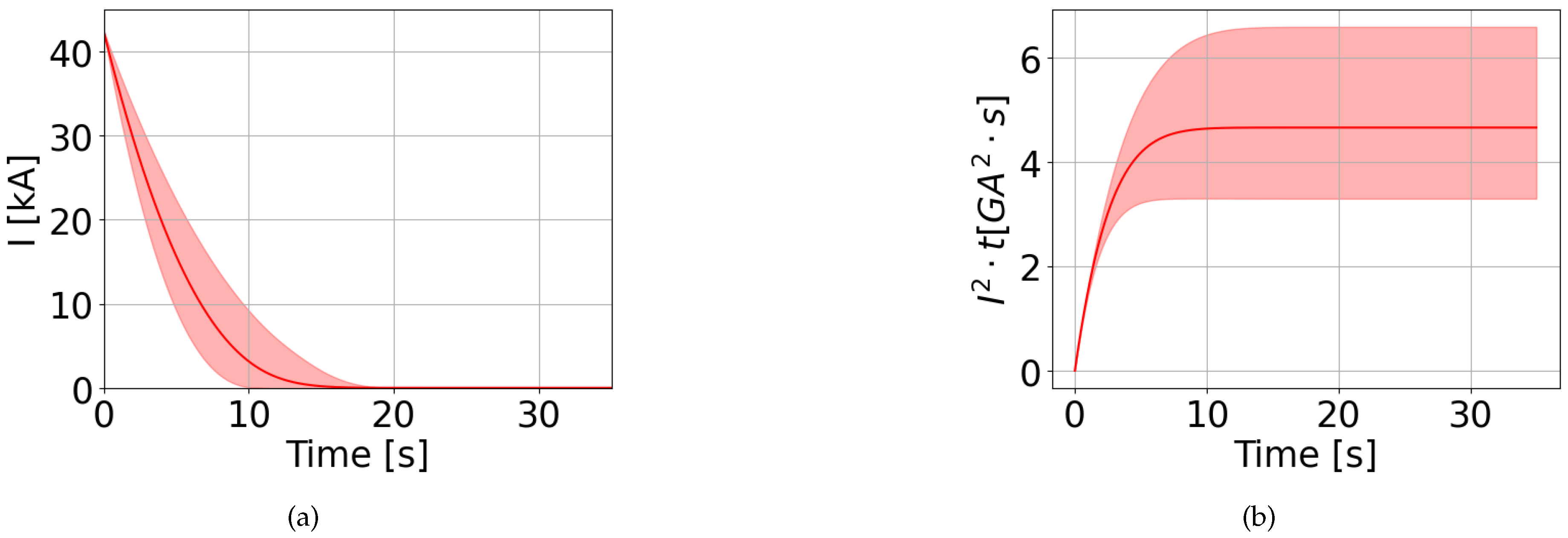
Figure 5. Statistical distribution of (a) peak of the power deposition and of (b) deposited energy, obtained using PCE with quadrature order 3.

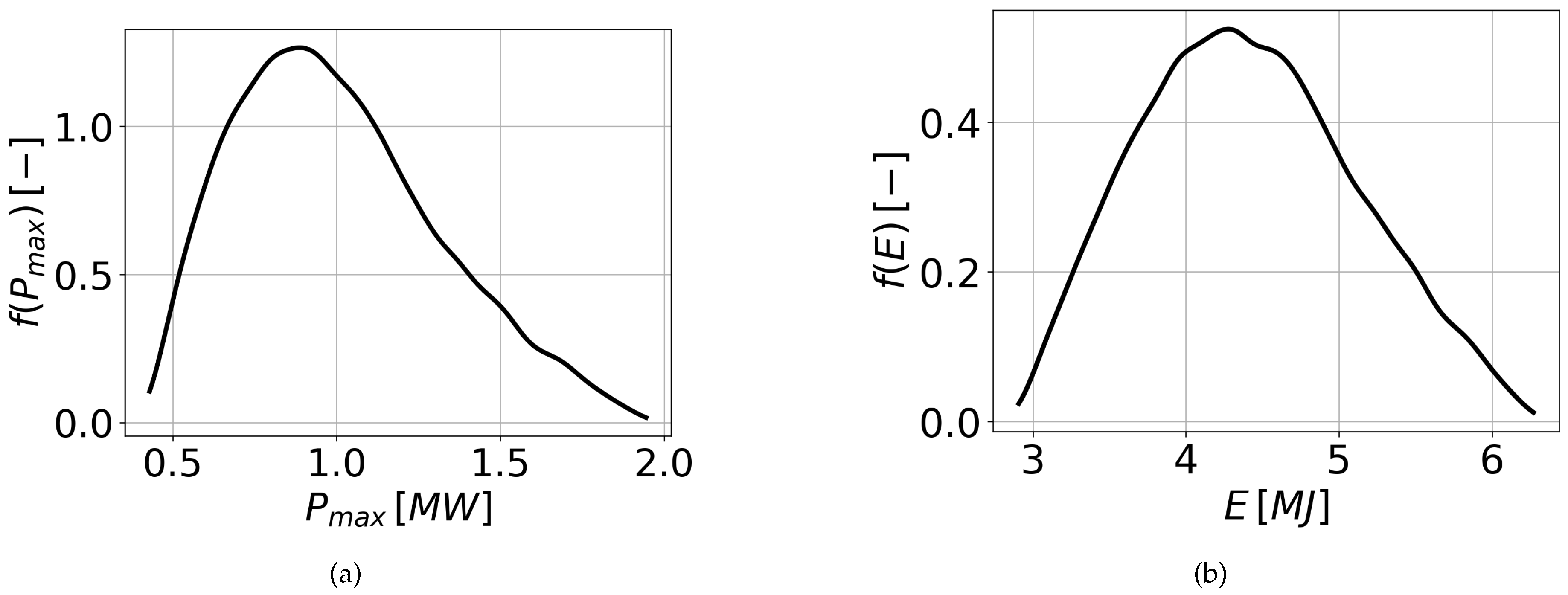
Figure 6. Average evolution of the power deposited within the TF coil casing with its

1 - 99 %

confidence range evaluated with PCE.

Figure 6. Average evolution of the power deposited within the TF coil casing with its

1 - 99 %

confidence range evaluated with PCE.

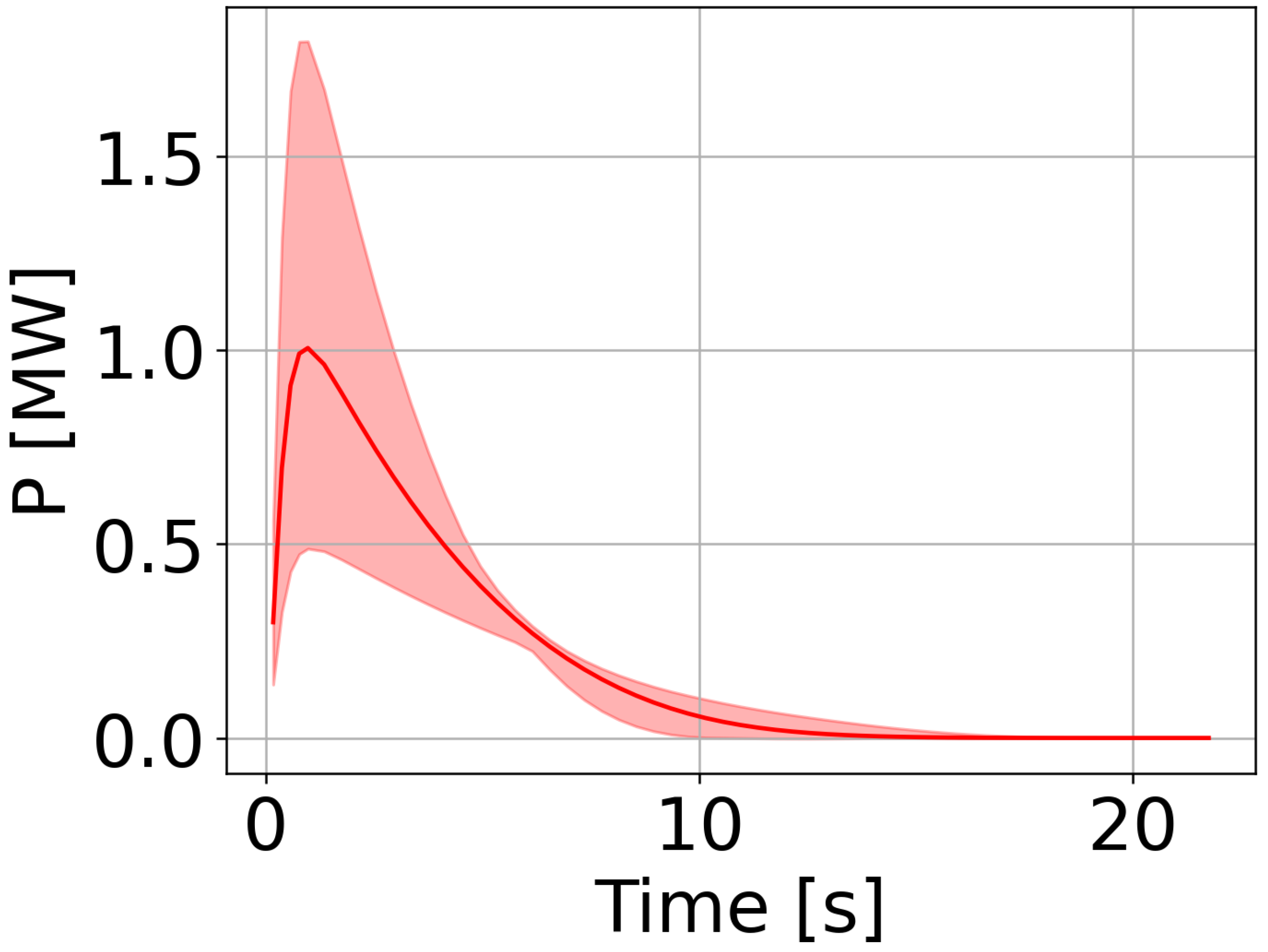
Figure 7. Map of (a)

τ

and (b) energy deposited in the coil casing in the

K, β

plane.

Figure 7. Map of (a)

τ

and (b) energy deposited in the coil casing in the

K, β

plane.

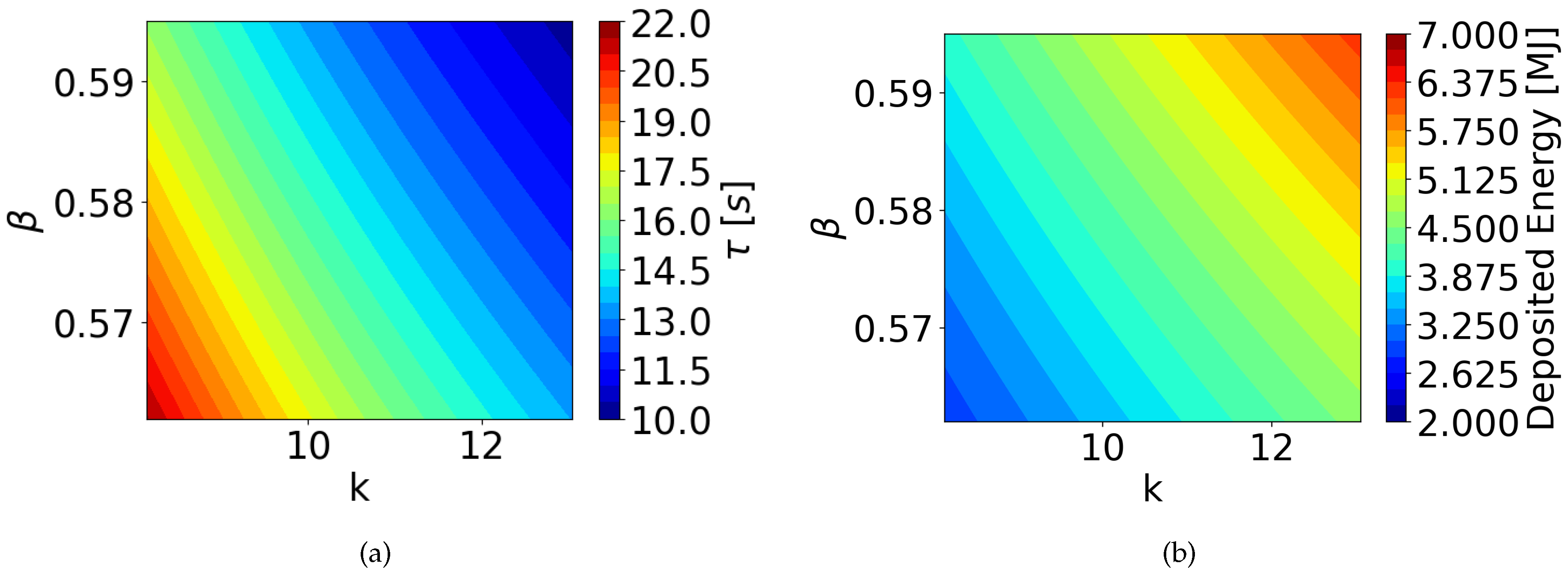
Figure 8. Evolution of (a) current and (b) total power deposited in the coil casing during the two WCSs.

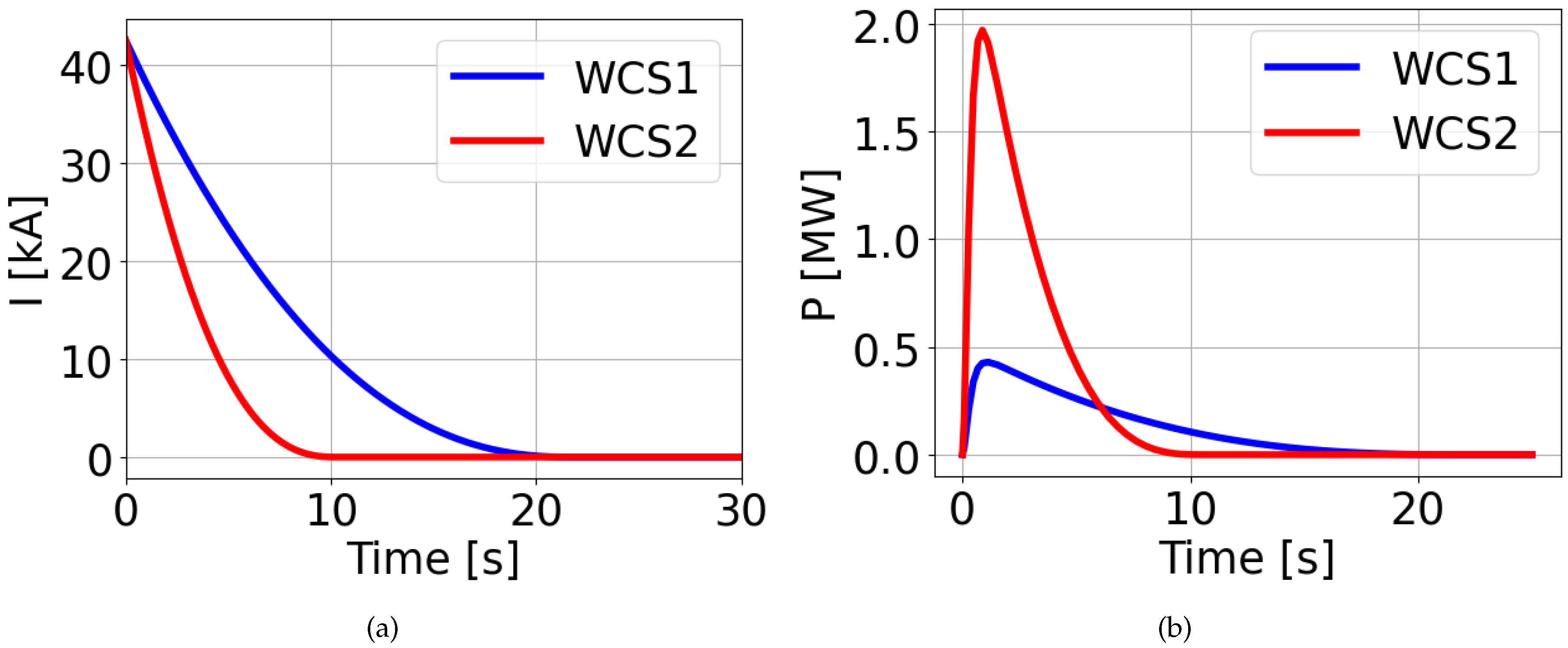
Figure 9. Voltage evolution computed in pancakes 5, 6 and 7 in both WCS1 and WCS2. The current evolution for WCS1 (solid) and WCS2 (dashed) is also plotted, to be read on the right axis.

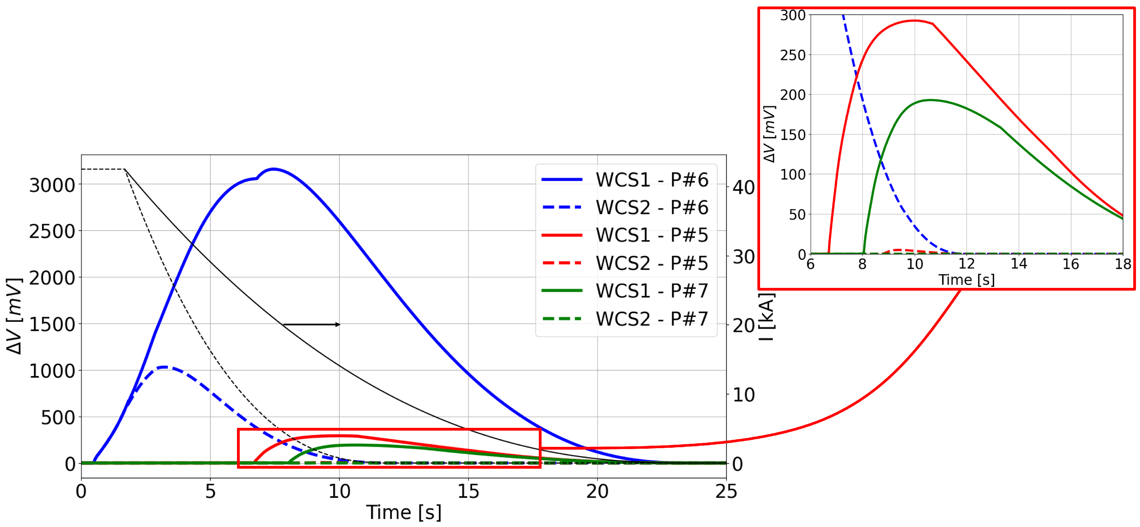
Figure 10. Maximum hot spot temperature reached in each pancake during the transient, for both WCS1 and WCS2.

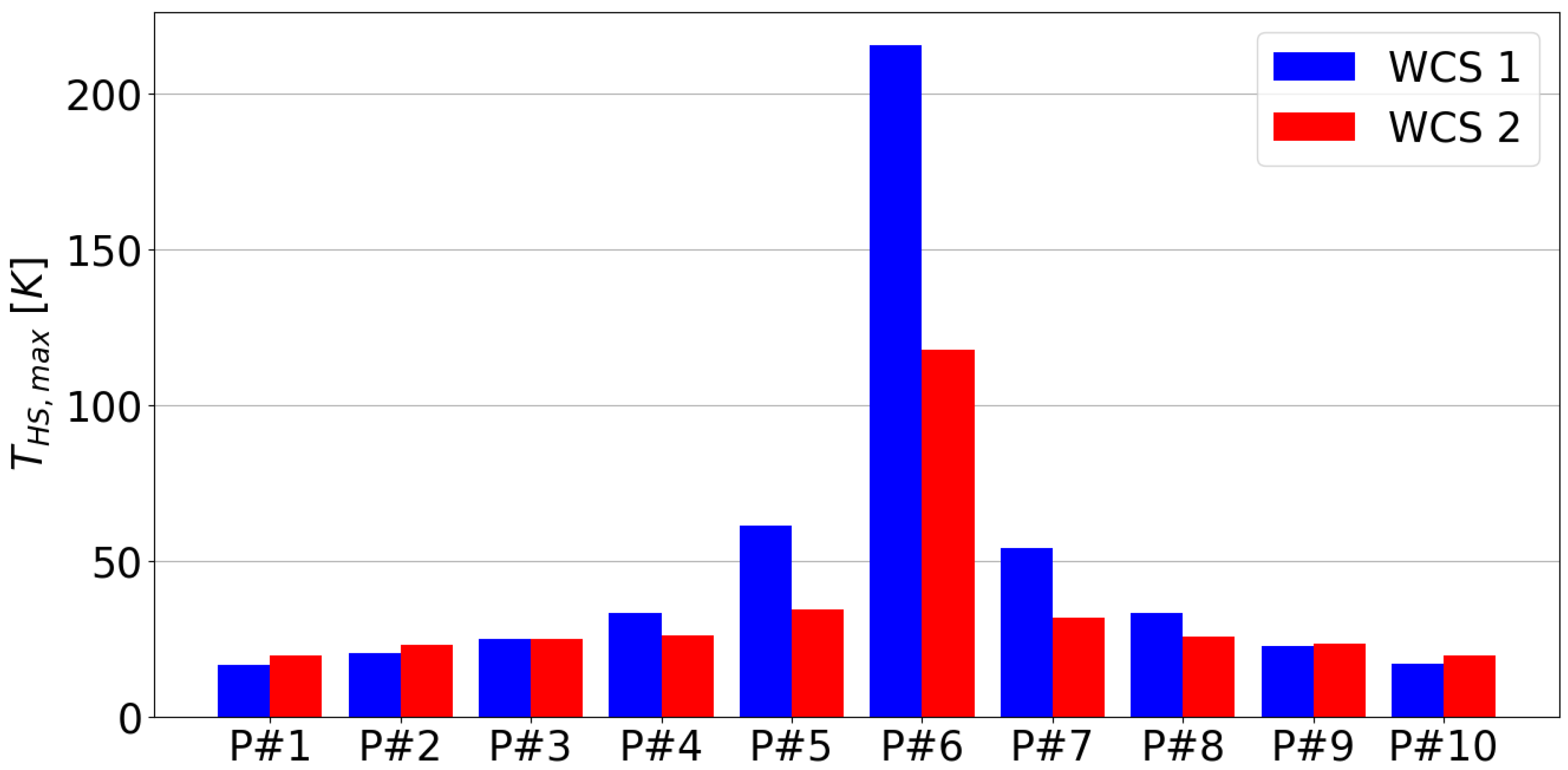
Table 1. Comparison between the mean value and standard deviation of the monitored variables using the MC, PCE and UT methods.

Variable	$\bar{V} \pm 2 \cdot σ$
	MC	PCE	UT
$τ [s]$	$14.77 \pm 4.70$	$14.76 \pm 4.69$	$14.77 \pm 4.69$
$Δ V_{F D U} [V]$	$5065.85 \pm 1708.03$	$5067.26 \pm 1708.40$	$5067.27 \pm 1698.46$
$Δ V_{T F} [V]$	$843.98 \pm 284.56$	$844.21 \pm 284.62$	$844.22 \pm 282.97$
$I^{2} \cdot t [G A^{2} \cdot s]$	$4.67 \pm 1.58$	$4.67 \pm 1.57$	$4.67 \pm 1.57$

Table 2. Comparison between the mean value and standard deviation of the peak power and the deposited energy evaluated with PCE and UT.

Variable	$\bar{V} \pm 2 \cdot σ$
	PCE	UT
$P_{m a x} [M W]$	$1.01 \pm 0.62$	$1.00 \pm 0.61$
$E [M J]$	$4.42 \pm 1.40$	$4.42 \pm 1.40$

Table 3. Comparison between the peak power obtained using the 3D-FOX and the PCE metamodel using as input the UT sigma points (

σ

) as input parameters.

Table 3. Comparison between the peak power obtained using the 3D-FOX and the PCE metamodel using as input the UT sigma points (

σ

) as input parameters.

	$P_{m a x, 3 D - F O X}$ [MW]	$P_{m a x, P C E}$ [MW]	Relative Error - $ε_{P_{p e a k}}$	$E_{3 D - F O X}$ [MJ]	$E_{P C E}$ [MJ]	Relative Error - $ε_{E}$
$σ_{1}$	$0.975$	$0.977$	$+ 0.28 %$	$4.40$	$4.40$	$- 0.03 %$
$σ_{2}$	$0.628$	$0.625$	$- 0.45 %$	$3.51$	$3.51$	$- 0.11 %$
$σ_{3}$	$0.726$	$0.728$	$+ 0.31 %$	$3.82$	$3.82$	$+ 0.01 %$
$σ_{4}$	$1.39$	$1.39$	$+ 0.28 %$	$5.28$	$5.28$	$+ 0.02 %$
$σ_{5}$	$1.30$	$1.30$	$+ 0.05 %$	$5.08$	$5.07$	$- 0.06 %$

Disclaimer/Publisher’s Note: The statements, opinions and data contained in all publications are solely those of the individual author(s) and contributor(s) and not of MDPI and/or the editor(s). MDPI and/or the editor(s) disclaim responsibility for any injury to people or property resulting from any ideas, methods, instructions or products referred to in the content.

© 2023 by the authors. Licensee MDPI, Basel, Switzerland. This article is an open access article distributed under the terms and conditions of the Creative Commons Attribution (CC BY) license (http://creativecommons.org/licenses/by/4.0/).

Copyright: This open access article is published under a Creative Commons CC BY 4.0 license, which permit the free download, distribution, and reuse, provided that the author and preprint are cited in any reuse.

MDPI Initiatives

Important Links

Choose an area of interest and we will send you notifications of new preprints at your preferred frequency.

Disclaimer

Application of the Polynomial Chaos Expansion to the Uncertainty Propagation in Fault Transients in Nuclear Fusion Reactors: DTT TF fast current discharge

Abstract

1. Introduction

2. Methodology

2.1. Electrical model

2.2. Electro-Magnetic model

2.3. Thermal-hydraulic model

2.4. Uncertainty propagation analysis

2.4.1. Polynomial Chaos Expansion

2.4.2. Unscented Transform

3. Results

3.1. Results of the Electrical model

3.2. Results of the Electro-Magnetic model

3.3. Identification of the worst case scenarios

3.4. Results of the Thermal-Hydraulic model

4. Conclusions and perspective

Author Contributions

Conflicts of Interest

References

MDPI Initiatives

Important Links

Subscribe