Submitted:
06 January 2024
Posted:
18 January 2024
Read the latest preprint version here
Abstract
Permafrost thaw is an important aspect of Earth's carbon cycles. Initial estimates suggest that permafrost thaw could contribute anywhere between 20 to 500 Gt of CO2-eq by 2100. These estimates are all fundamentally centered around one number: active layer thickness (ALT). The deeper the ALT, the more emissions. Unfortunately, ALT is a highly spatially heterogeneous number and determined by numerous thermal, soil hydrology, and geomorphological effects. The remotely sensed active layer thickness (ReSALT) algorithm was introduced in 2010 to provide scientists with a way to model ALT heterogeneously at meter-scale resolution. However, upon inspection, this work shows that ReSALT's modeling approach is self-inconsistent. This work then introduces SCReSALT (Self-Consistent ReSALT) to solve that problem. Experimental comparisons to a past study in Utqiagvik (formerly Barrow), Alaska show significant improvement and suggest that SCReSALT should replace ReSALT. Code to reproduce all results can be found at https://github.com/jmathur25/permafrost-prediction.
Keywords:
synthetic aperture radar
; interferometric synthetic aperture radar
; permafrost thaw
; climate change
1. Introduction
Climate forecasting studies estimate that permafrost thaw could contribute anywhere between 20 to 500 Gt of CO2-eq by 2100 ([1,2,3,4]). These estimates varied in the phenomenon they modeled, how that phenomenon was modeled, and assumptions of warming trends, therefore explaining the wide range of predictions. Regardless of these differences, a crucial variable in all forecasts is the active layer thickness (ALT), which describes the topmost layer of permafrost subject to annual freeze and thaw. Warmer temperatures lead to deeper active layers. Organic carbon is distributed throughout the soil column, meaning deeper active layers permit microbacteria to process more carbon and emit more greenhouse gases. Hence, there is a strong interest in developing modeling and forecasting algorithms for ALT. For more background on permafrost carbon cycles, the reader is referred to [5].
2. Background
2.1. ReSALT Description
The remotely sensed active layer thickness (ReSALT) algorithm was introduced to model ALT with broad spatial coverage while preserving heterogeneous predictive power [6]. Without remote sensing, our understanding of permafrost thaw is constrained to sparse in-situ observations. Given the vast extent of permafrost, it would be incredibly useful if remote sensing could accurately monitor ALT. ReSALT leverages a technique known as interferometric synthetic aperture radar (InSAR) to create its predictions. For background information on InSAR, the reader is referred to [7]. For the purpose of analysis in this paper, an InSAR measurement should be thought of as having three properties: i) the date of the reference SAR acquisition, ii) the date of the secondary SAR acquisition, and iii) a geocoded image containing ground subsidence1 per pixel. Specifically, if the ground position is measured as in an unchanging, earth-centered reference frame and the positive direction points towards the Earth’s center, then the image will consist of per pixel.
ReSALT has been used in several studies since its conception, such as in [6,8,9,10]. While it has demonstrated promising results, there is room for improvement. For example, the Permafrost Dynamics Observatory project reported a root mean square error (RMSE) of 15.18 cm in ReSALT predicted vs in-situ ALTs [10]. The in-situ data had an average ALT between 50 and 60 cm, making the RMSE significantly large with respect to the unit of measure. This large error served as motivation for this paper.
ReSALT is based on two main phenomena. The first is that thaw depth is proportional to , where stands for Accumulated Degree Days of Thaw. This is the well-known Stefan Equation and is shown in (1).
where N is a proportionality factor. This is derived in Appendix A. The second phenomenon is that the soil is fully saturated, meaning all pore space is filled with water. Consequently, when ice thaws into liquid water, the amount of volume reduces, which leads to ground subsidence. This is shown visually in Figure 1 and mathematically in (2).
where is the density of water, is the density of ice, P is the soil porosity, and S is the soil saturation. The integral captures the volumetric water content. The ratio describes the difference in volume height when the ice phase transitions to liquid water per unit volume of ice.2 The ground subsidence can be computed by multiplying the two quantities, therefore arriving at (2). f is introduced as a convenience to compute subsidence from thaw depth.
Any particular InSAR image contains subsidence difference . Temperature is typically known at a coarse resolution. Hence, ReSALT strives to find a way to relate these two quantities, and ultimately retrieve . It does so by posing the following least-squares inversion problem:
where is the measured subsidence difference in the ith interferogram, and describe the times of the two SAR acquisitions that were used to create the ith interferogram, and and describe the ’s for and . Note that all refer to the same geographic location, but may differ in pixel location from image to image. R and E are the unknown variables and are solved for. R captures a long-term subsidence trend. More information can be found in [6,11]. E captures the relationship between and subsidence difference, which can then be used to identify subsidence at any arbitrary time t via:
Then, (2) can be inverted to obtain . More details on ReSALT’s derivation are shown in Appendix B.
2.2. ReSALT Inconsistency Description
In (4), subsidence is modeled as proportional to . Using (1) and (2), it becomes evident that this only happens when P is constant with depth. Hence, any application of ReSALT that uses a non-constant porosity model is self-inconsistent. Examples of self-inconsistent applications of ReSALT are [8] and [9], which use the “mixed soil model” shown later in this paper.
3. Method
Observe that if R is ignored, the correct inversion LHS (left-hand side) for (3) is thaw depth difference:
However, only subsidence difference and are measured. To see if subsidence difference can be related to thaw depth difference, (1) is analyzed as a ratio:
For convenience, is introduced. Next, a list of candidate on some large interval of possible thaw depths is generated, and corresponding is computed using (7). The subsidence for each candidate and can be computed using (2). A plot of candidate thaw depth differences and corresponding subsidence differences can then be constructed. See Figure 2 for examples of this plot for two soil porosity models. Each of these models is explained in [8]. As shown in the bottom two figures, a particular subsidence difference can unambiguously be mapped to a thaw depth difference. Intuitively, this is because (7) enables multiplicative growth of with respect to . Consequently, the hope is that (2) enables subsidence difference to grow strictly monotonically. Put another way, for each interferogram, Q (which is known) acts as a constraint parameter that helps search the space of possible thaw depth pairs and . Corresponding subsidences can be computed and a graph can depict whether subsidence difference can be related to thaw depth difference. Of course, there is no guarantee this will work for all soil porosity models. A counterexample is discussed in Section 3.1. Lastly, note that in Figure 2 the bottom images demonstrate the effect of Q on the method’s robustness. For the constant porosity model, there is no effect because the thaw depth difference is linearly related to the subsidence difference. For the “mixed soil model,” the slope is higher in the bottom-left image, making it easier to identify a particular thaw depth difference from a given subsidence difference. This is expected because larger Q ratios make the thaw depth pair have smaller values for the same thaw depth difference. Smaller thaw values exhibit larger subsidence gradients, as the top-right plot shows.
This method is summarized in Algorithm 1. (3) can be rewritten as:
| Algorithm 1 Self-Consistent ReSALT LHS Retrieval |
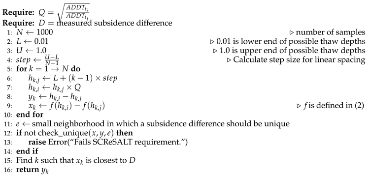 |
where is the best-matching thaw depth difference reported for each via Algorithm 1. This now forms a self-consistent modeling of thaw, temperature, and ground subsidence. Hence, this new method is called SCReSALT (Self-Consistent ReSALT). Least-squares inversion gives the best N. This is the same N as in (1), which can then be used to find the thaw depth at any point in the thaw season.
To extend the formulation to multiple years, the long-term trend R must be discounted from before following the above approach. ReSALT jointly inverts for R and E, but a self-consistent model cannot do that. So, R must be estimated independently of and prior to N. This work does not explore R estimation with SCReSALT experimentally. Here are some possible solutions, but exploring them is left to future work:
- Form interferograms across multiple years at the start of the thaw season, ideally when . Any observed subsidence can be attributed to R. Compute the best-fit R that solves all .
- Compute an initial estimate of N by solving (8). N could be solved either per thaw season (which makes ) or overall. Then, like the previous bullet point, form interferograms across multiple years at the start of the thaw season and remove the subsidence contribution due to any initial thaw. This is known because the subsidence contribution due to initial thaw can be written as: . Note denotes N for the thaw season in the 2nd SAR image in the ith interferogram. means the same for the 1st SAR image. Compute the best-fit R that solves all .
Once R is known, the multi-year problem can be solved using (8) but instead of giving Algorithm 1 the observed subsidence difference , give it .
For completeness, it is worth noting that both ReSALT and SCReSALT do not need both SAR acquisitions to be during the thaw season. One acquisition could be before the thaw season, in which case can be assumed for that acquisition. Hence, any measured subsidence difference can be modeled as the true subsidence at that point. ReSALT can directly use (3). SCReSALT would need a slight modification because it operates using ratios. Algorithm 1 could be modified such that if , simply report . Similarly, if , report . The negative sign is because is the subsidence underwent when going from to . That is expected to be positive if and negative vice-versa.
3.1. SCReSALT Counterexample Discussion
In Appendix C, a counterexample that does not meet the SCReSALT requirement is derived. Some possible solutions are described below, but exploring them is left to future work.
- From multiple interferograms per year and obtain time-series measurements of subsidence difference. Attempt to interpolate the measurements onto a subsidence difference vs thaw depth difference graph and determine which thaw depth differences best explain the data.
- Make sure to get a SAR acquisition before the thaw season starts. This allows one to treat the subsidence difference as the true subsidence. Handling this is easy and was described earlier in this paper.
- Using a prior on thaw depth difference might isolate a thaw depth difference as the most likely candidate.
Importantly, any soil porosity model can be tested to see if it meets the SCReSALT requirement using Algorithm 1. Only then would exploring these options be necessary.
4. Experiments
To assess the practical improvement of SCReSALT, it is benchmarked against the results reported in [9]. [9] applies ReSALT to Utqiagvik (formerly Barrow), Alaska and uses the “mixed soil model” to predict ALT from 2006 to 2010. Metrics are extracted from the paper and the data product they release, which can be found at https://daac.ornl.gov/ABOVE/guides/ReSALT_InSAR_Barrow.html. [9] uses data from the U1 CALM3 plot. It uses ALOS-PALSAR L-band data and generates interferograms using the ISCE2 framework4. The paper defines the metric:
where e is the uncertainty in the measurement. In [9], cm. If , it is called a “great match.” If the is within the uncertainty of , it is called a “good match." Otherwise, it is called a “bad match.” Uncertainty analysis is not described in this paper, but in brief, it could be computed by assigning an uncertainty distribution to each ReSALT/SCReSALT parameter and either analytically propagating that into an uncertainty in the prediction or more practically using numerical simulation. This work uses the fact that [9] stated that the ReSALT uncertainty is roughly twice that of the measurement uncertainty. Hence, cm. Other experimental details are described in Appendix D. With those details explained, results are shown in Table 1.
5. Results
The metrics reported in [9] closely match the results computed from the data product. The “good match” category is a little worse because is not precisely known. That then influences the “bad match” category. Otherwise, the alignment is high, meaning there is high confidence in the derived Pearson R, mean absolute error (MAE), and RMSE values. The author also attempted to reproduce ReSALT results but generally had worse numbers. It is difficult to get precise replication without source code, which is not available for [9]. Regardless, SCReSALT is shown to outperform ReSALT on virtually all metrics and handles outliers better given its reduced RMSE and . If compared to the reproduced ReSALT, SCReSALT’s improvement is even stronger. It is also worth discussing the ReSALT data product’s low Pearson R. It is not clear why, but given the high value of , it is possible to have many “great matches” despite no correlation between predicted and ground-truth ALTs.
6. Conclusion
This work presents SCReSALT, a modification to ReSALT that enables consistent modeling of thaw, temperature, and ground subsidence. It describes the conditions where SCReSALT can be used and shows its applicability to previously developed soil models. A counterexample to SCReSALT is also derived. Possible solutions are discussed, but exploring them is left to future work. Experimentally, SCReSALT demonstrates significant improvement in estimating ALTs in Utqiagvik, Alaska. The author recommends that SCReSALT become a standard tool in permafrost thaw modeling.
Conflicts of Interest
The author declares no conflicts of interest.
Appendix A. Stefan’s Equation Derivation
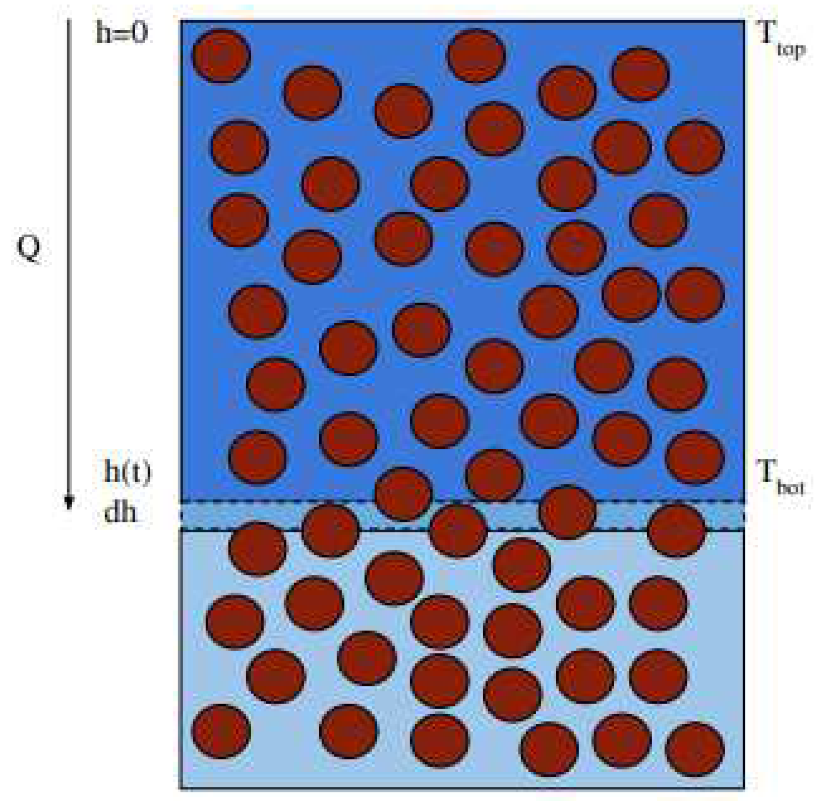
First, Stefan’s Equation is derived to understand the relationship between temperature history and ground ice thaw. Figure 3 is provided to help visualize the relevant processes.
Figure 3.
A diagram of a thawing soil column. h denotes the position of the thaw front. Q is the (uniform) heat flux induced by and . is the same as the temperature of the air. Brown circles denote soil particles. Anything that is not a soil particle is pore space. Note that any real soil would have a far more dense concentration of soil particles. Dark blue denotes liquid (thawed) water. Light blue denotes frozen (unthawed) water. If this is being viewed without color, the thawed water is above the middle small dashed rectangle, while the frozen water is below it. In this diagram, it is assumed that all pore space is filled with water. This does not have to be the case for Stefan’s equation to apply. A different bulk density and latent heat of thaw L can capture the thaw dynamics of a variety of soil hydrology models.
The derivation begins with Fourier’s Law:
where Q is the heat per unit area per unit time, is the thermal conductivity, T is temperature, and h defines the position of the thaw front. Note that both T and h are functions of time t. Assuming the temperature gradient is uniform throughout the column:
Next, it is assumed that all heat is absorbed as latent heat to facilitate phase change from ice to liquid water. Consequently, an infinitesimal change in thaw depth can be related to the amount of heat required to do so by:
where H is the amount of heat per unit area required to advance the thaw front by , is the bulk density of soil, and L is the latent heat of thawing. Differentiating with respect to time:
Since refers to the boundary of thawed/frozen soil, it is reasonable to assume 5, in which case it can removed from (16).
Practically, once the thaw season begins . Since is typically measured on a daily basis (rather than continually), the right-hand side (RHS) can be replaced with:
where stands for the Accumulated Degree Days of Thaw. It is a standard number used in permafrost literature and is calculated at any day t by summing the temperatures larger than 0 of all days preceding and including t. Now, looking at the LHS, and L are assumed to be constant with depth:
Appendix B. ReSALT Derivation
The derivation for ReSALT is now presented. First, is it assumed that thaw begins when first exceeds 0°C-days.6 So, if is the start of the thaw season, it is known that , . Recall that (21) only applies for times within the thaw season, so that is why this assumption is needed. The thaw depth at any time can then be written as:
(1) is now derived (). InSAR gives measurements of ground subsidence as determined by two SAR acquisitions at and . ReSALT models subsidence using (2). In general, P is not constant with depth. This means is not linearly proportional to . However, because only and D are measured, ReSALT strives to find a way to relate the two. To do so, it assumes proportionality:
This is the assumption, or self-inconsistency, that this paper solves. Continuing with the derivation, this is subsituted into (5):
Appendix C. SCReSALT Counterexample Analysis
A more rigorous analysis of SCReSALT is now conducted through which a counterexample is derived. The mathematical premise of SCReSALT can be stated as follows: Given an integrable7 function P for which , then for any ratio , can be uniquely identified by . This can be restated as: if , then SCReSALT requires . Note that f is strictly increasing with z. The porosity can be written as:
There are constraints on P, and hence constraints on f, but for convenience P is initially ignored. To create a convincing failure case, the following is needed:
for some arbitrary Q and . A simple way to analyze this is to consider a piecewise linear f:
This condition can certainly be constructed. A quadratic function can fit the ends of the piecewise linear function to ensure f is always differentiable. As long as i) the values and derivatives match at the intersection points, ii) f is strictly increasing, and iii) a valid P can be constructed from f, the conditions are met. An example is shown below:
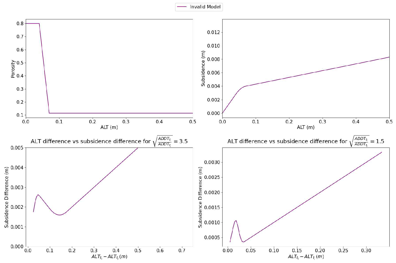
This example is scaled such that there is a valid corresponding P model, which can be computed using (27). Both f and P are visualized in Figure 4, which demonstrates a potentially realistic soil porosity model that does not meet the SCReSALT requirement.
Figure 4.
A diagram showing a physically realizable soil porosity model that fails the SCReSALT requirement. As shown in the bottom images, subsidence difference cannot necessarily be equated to an ALT difference.
Figure 4.
A diagram showing a physically realizable soil porosity model that fails the SCReSALT requirement. As shown in the bottom images, subsidence difference cannot necessarily be equated to an ALT difference.
Appendix D. Additional Experiments Info
The paper uses node 61 of the U1 CALM plot as a reference or calibration node. In general, InSAR requires a calibration pixel where subsidence is known or can be assumed to calibrate the entire subsidence image. For example, exposed bedrock and gravel are typically assumed to have 0 subsidence. In [9], no pixel had known subsidence, so they instead formulated (3) as a delta subsidence difference with respect to the calibration node. They then scaled the best-fit E (really a delta E) by the at measurement time, which is a valid operation under ReSALT formulation (but not SCReSALT). Then, they calculated the expected subsidence of the calibration node by evaluating (2) on the calibration node’s in-situ ALT. An offset is applied to make the calibration node E align with its expected subsidence. At this point, subsidence at measurement time is known per pixel. Finally, by inverting (2), ALT is estimated per pixel. SCReSALT handles the calibration node as follows:
- SCReSALT is given the seasonal ALT of the calibration node as input. This is computed from the measured in-situ ALT and scaled to the end-of-season thaw depth according to (7). Note that is known at measurement time and end-of-season time, so this scaling is possible.
- For a particular InSAR image, the seasonal ALT of the calibration node is scaled twice using (7), once using the at the time of the reference image to get and another using the at the time of the secondary image to get . Using (2), and are computed. Then, the expected subsidence difference can be computed as . This is used to apply a global offset to the InSAR image such that the calibration pixel has the expected subsidence difference.
- SCReSALT operates with the calibrated subsidence difference image.
To be clear, the steps listed above only need to be followed when the calibration node is itself subsiding according to (2). If there was an exposed bedrock or gravel pixel, then a simple procedure would suffice where a global offset is applied to make the calibration pixel have 0 subsidence difference. SCReSALT ultimately needs an image in which subsidence difference is known. This is the same as ReSALT.
There are a few final experimental details that need mentioning:
- The U2 plot was used in [9] but not in this paper. It accounted for a single pixel while U1 contributed 121 pixels (minus 6 unused pixels and 1 calibration pixel). This extra data point shouldn’t affect the analysis too much. Note that this would not affect the comparison between the ReSALT data product and SCReSALT in Table 1 because the ReSALT data product ALTs were only compared to U1 CALM ALTs.
- Some interferograms were listed incorrectly in Table A1 of [9]. For example, rows 7 and 9 have the same granules but different dates. Duplicating granules does not make any sense, so this is a typographical error. The dates were used to infer the correct granules. The modified interferogram list is part of the publicly released codebase.
- The 20th interferogram encountered a processing error with ISCE2. Given that this was just 1 interferogram out of 20, it is not expected to affect the analysis too much.
References
- Schaefer, K.; others. Amount and timing of permafrost carbon release in response to climate warming. Tellus B 2011, 63, 165–180. [Google Scholar] [CrossRef]
- Schneider von Deimling, T.; others. Observation-based modelling of permafrost carbon fluxes with accounting for deep carbon deposits and thermokarst activity. Biogeosciences 2015, 12. [Google Scholar] [CrossRef]
- Ruiz, S. $41M audacious grant will tackle permafrost thaw. Woodwell Climate, 2022. Available at: https://www.woodwellclimate.org/41-million-grant-for-permafrost-thaw-monitoring/.
- Carbon emissions from Permafrost. 50x30, 2023. Available at: https://www.50x30.net/carbon-emissions-from-permafrost.
- Miner, K.; others. Permafrost carbon emissions in a changing Arctic. Nature Reviews Earth & Environment 2022, 3. [Google Scholar] [CrossRef]
- Liu, L.; others. InSAR measurements of surface deformation over permafrost on the North Slope of Alaska. Journal of Geophysical Research: Earth Surface 2010, 115. [Google Scholar] [CrossRef]
- European Space Agency. InSAR Principles: Guidelines for SAR Interferometry Processing and Interpretation. Technical report, ESA Publications, 2007.
- Liu, L.; others. Estimating 1992–2000 average active layer thickness on the Alaskan North Slope from remotely sensed surface subsidence. Journal of Geophysical Research: Earth Surface 2012, 117. [Google Scholar] [CrossRef]
- Schaefer, K.; others. Remotely Sensed Active Layer Thickness (ReSALT) at Barrow, Alaska Using Interferometric Synthetic Aperture Radar. Remote Sensing 2015, 7. [Google Scholar] [CrossRef]
- Chen, R.; others. Permafrost Dynamics Observatory (PDO) – Part II: Joint Retrieval of Permafrost Active Layer Thickness and Soil Moisture from L-band InSAR and P-band PolSAR. Earth and Space Science 2023, 10. [Google Scholar] [CrossRef]
- Nixon, F.; Taylor, A. Regional active layer monitoring across the sporadic, discontinuous and continuous permafrost zones, Mackenzie Valley, northwestern Canada. Proceedings of the 7th International Conference on Permafrost. International Permafrost Association, 1998, pp. 815–820.
- Michaelides, R.J.; others. Permafrost Dynamics Observatory—Part I: Postprocessing and Calibration Methods of UAVSAR L-Band InSAR Data for Seasonal Subsidence Estimation. Earth and Space Science 2021, 8. [Google Scholar] [CrossRef] [PubMed]
| 1 | InSAR measures subsidence in the line-of-sight (LOS) direction. That is usually projected from the vertical direction and can be converted into vertical deformation using the incidence angle. |
| 2 | [10] argues convincingly that the ReSALT formulation only works when . If , some open pore space will be filled by freeze/thaw before the ground subsides. At a critical threshold (characterized by the densities of liquid water and ice), freeze/thaw might lead to no ground subsidence. So, this work assumes . |
| 3 | CALM is a long-running program that collects data on permafrost thaw. Data can be accessed at https://www2.gwu.edu/~calm/
|
| 4 | |
| 5 | At this point, the temperature must be in Celsius. |
| 6 | [12] proposes that this is difficult to precisely know and suggests a different approach. However, that is not addressed here. |
| 7 | It could be argued that a physically realizable P should be differentiable. That is ignored in the analysis presented in this paper, but it not hard to see that the example P given later could be made differentiable without changing the conclusion. |
Figure 1.
The left box shows the soil column during winter when all water is frozen. The right box shows the soil column during summer when water is thawed up to the ALT. Subsidence occurs because ice takes up more volume than water for the same mass. Hence, under the assumptions of no water loss and fully saturated soil, ground subsidence is observed. Note that is typically measured with respect to the ground at the time of measurement. is typically not measured.
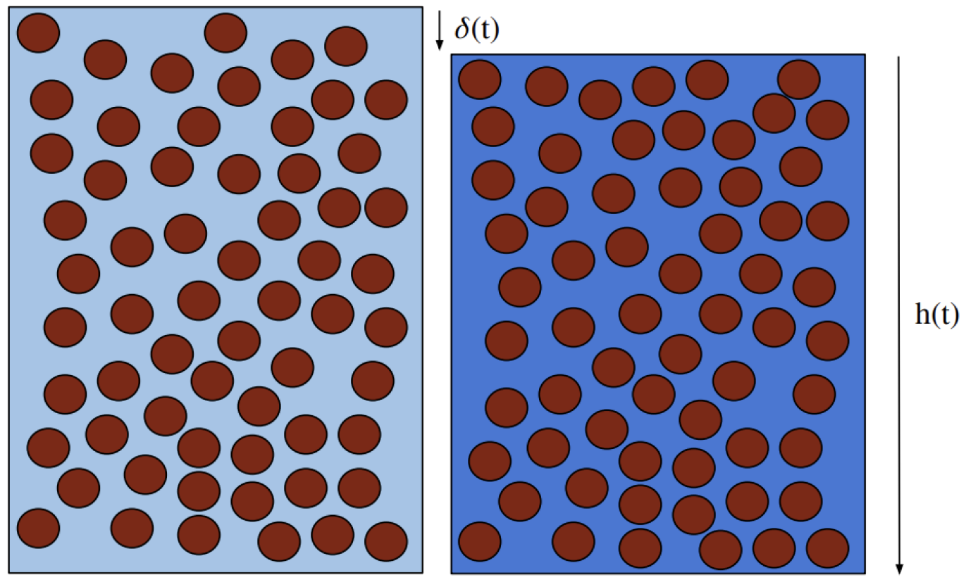
Figure 2.
Plots showing the core idea of SCReSALT.
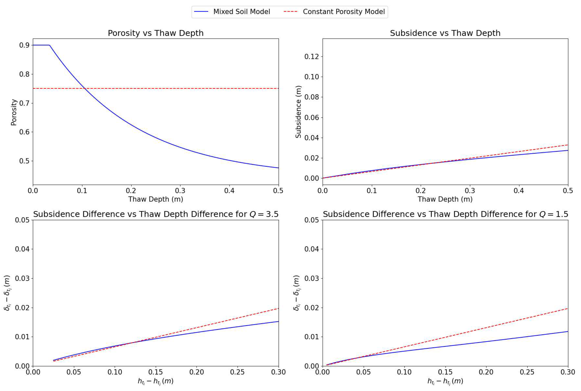

Table 1.
Comparison of ReSALT vs. SCReSALT performance. The double line separates results from [9] and those produced by the author. For each metric, the best score between ReSALT and SCReSALT is bolded. This is not done for great/good/bad match because they are codependent. Also, two nodes had invalid predictions for the reproduced ReSALT, so they were excluded. This slightly affects the comparison.
| Metric | ReSALT [9] | ReSALT (Data Product) | ReSALT (Reproduced) | SCReSALT |
|---|---|---|---|---|
| Avg | 2.5 | 2.543 | 3.039 | 1.833 |
| Great Match | 0.62 | 0.623 | 0.518 | 0.570 |
| Good Match | 0.26 | 0.228 | 0.205 | 0.290 |
| Bad Match | 0.12 | 0.1491 | 0.277 | 0.140 |
| Bias (m) | 0.008 | 0.007 | -0.067 | -0.020 |
| Pearson R | - | -0.284 | 0.324 | 0.300 |
| MAE (m) | - | 0.087 | 0.107 | 0.084 |
| RMSE (m) | - | 0.126 | 0.138 | 0.107 |
Disclaimer/Publisher’s Note: The statements, opinions and data contained in all publications are solely those of the individual author(s) and contributor(s) and not of MDPI and/or the editor(s). MDPI and/or the editor(s) disclaim responsibility for any injury to people or property resulting from any ideas, methods, instructions or products referred to in the content. |
© 2024 by the authors. Licensee MDPI, Basel, Switzerland. This article is an open access article distributed under the terms and conditions of the Creative Commons Attribution (CC BY) license (http://creativecommons.org/licenses/by/4.0/).
Copyright: This open access article is published under a Creative Commons CC BY 4.0 license, which permit the free download, distribution, and reuse, provided that the author and preprint are cited in any reuse.


