
Submitted:
05 December 2023
Posted:
06 December 2023
You are already at the latest version
Abstract
This paper elucidates the impact of uncertainty on the Markowitz asset allocation and how it performs. The findings imply that when evaluated out-of-sample, estimation errors in parameters might significantly affect how well an allocation performs. Numerous publications that address this ambiguity have been highlighted to emphasize our findings further. In our work, we compare these approaches to alternative allocation strategies and explain their performance in both expected and real out-of-sample events. We find that the Markowitz framework can be improved by using tactics that take uncertainty into account. Longer sample numbers, however, may not always translate into better outcomes. Applying a short-sale constraint can also enhance the initial portfolio. Finally, we find that even more basic approaches to asset allocation, such as equally weighted allocation, perform reasonably well.
Keywords:
Expected Events
; Equally Weighted Allocation
; Markowitz Asset Allocation
; Out-of-Sample Events
1. Introduction
According to an ancient Talmudic proverb, people should set aside three equal portions of their money: one for land, one for business, and one for storage. The concept of allocating your funds among various assets is referred to as "asset allocation". There are a wide range of professional viewpoints on the best approach to accomplish this, despite the fact that many have tried [1,2,3,4,5,6]. A scientist by the name of Markowitz made a substantial addition to this field in 1952. To determine the optimal approach to allocate your money among assets, he employed concepts such as covariances—a measure of how the returns of various assets relate to one another—and the standard deviation, which is a measure of risk. He discovered that the least risky portfolio for a given projected return is the optimal one. The estimates utilized for variances, covariances, and expected returns, however, have an impact on this approach. Stated differently, the precision of these approximations is critical; otherwise, the model may not perform as intended in practice. "Parameter uncertainty" is another term for this problem of ambiguous estimations. This raises a few crucial queries:
- How can the Markowitz framework’s uncertainty be explained?
- Does the model perform better when uncertainty is considered?
- How do these optimized allocations stack up against alternative tactics?
- Can the model do better with more data?
- Is it feasible to make a trustworthy performance prediction?
- Does performance improve when there are limitations on allocation?
In this study, I investigate different approaches to asset allocation that try to deal with this ambiguity about the parameter. I compare these options against the original model as well as alternative approaches such as the “1 over N” strategy. I consider both the real-world performance and the expected performance. I also provide a topic that has not received much attention: short-sale limits on assets. I also suggest a model extension that takes parameter uncertainty into account. To be sure the results are trustworthy, I run my analyses on two distinct sets of data.
The paper is as follows: In Section 2, the Markowitz model’s theoretical foundation and constraints are covered. Whereas Section 3 investigates model extensions for stronger allocations based on related works. The empirical analysis is covered in Section 4. I give my findings and methodologies, as well as the sources of our data in Section 5 and Section 6. I evaluate the various asset allocation approaches in both simulated and actual environments in Section 7. My study is concluded in Section 8, which discusses my analysis and their results.
2. Background: The Mean-Variance Model, Criticism and its Extensions
2.1. The Asset Allocation According to Markowitz
The classic asset allocation problem in finance involves an investor seeking to distribute their initial wealth, denoted as , among N risky assets, with returns assumed to follow a normal distribution characterized by expected rates of return () and a variance-covariance matrix (). The investor’s goal is to determine the optimal portfolio () that maximizes their expected final wealth, given their preferences quantified by a utility function, typically the Constant Absolute Risk Aversion (CARA) utility function. The CARA utility function, , reflects the investor’s profit-seeking and risk-averse nature. The CARA parameter, k, represents the investor’s risk tolerance. A positive k implies an upward-sloping utility function, becoming less steep as wealth increases, aligning with the investor’s preference for higher wealth and aversion to risky prospects. Assuming normal distribution of returns, the final wealth (W) is also normally distributed with mean and variance . The optimization problem for the rational investor involves maximizing expected satisfaction or utility, given by , leading to the mean-variance criterion:
Here, represents the investor’s risk aversion, with higher values indicating stronger aversion to variance. The optimization, known as the mean-variance criterion, is crucial for portfolio selection, considering both expected returns and risk. In a one-fund setting, where investors can only invest in risky assets, the optimization simplifies. However, in a two-fund setting, a risk-free asset is introduced, expanding the model. The investor now allocates wealth between the risky portfolio and the risk-free asset, considering the risk-return trade-off. In the mean-variance framework, the investor seeks to balance risk and return to achieve the most favorable outcome. The utility function’s exponential form reflects diminishing marginal utility of wealth, capturing the investor’s aversion to risk. The model helps investors make informed decisions on portfolio allocation, balancing risk and reward based on their risk preferences. The analysis also highlights the importance of the risk aversion parameter, , in the decision-making process. A higher implies a lower tolerance for risk, leading to a more conservative investment strategy. The mean-variance criterion provides a quantitative approach to portfolio optimization, aligning with the principles proposed by Markowitz.
2.2. Mean-Variance Efficient Portfolios in a One-Fund Setting
The mean-variance framework, introduced by Harry Markowitz in 1952, offers a solution for optimal asset allocation in the absence of a risk-free asset. At its core is the concept of the efficient frontier, a curved line on a risk-return graph that represents the optimal balance between expected portfolio return and standard deviation. This model capitalizes on the benefits of diversification by combining assets with less than perfect correlation, thereby reducing idiosyncratic risks. The goal is to determine the optimal weights for each asset in the portfolio to minimize overall risk. For a given expected return, denoted as µ¯, the mean-variance efficient portfolio aims to minimize the portfolio’s risk, subject to constraints. The Lagrange function is employed to solve the optimization problem, incorporating Lagrange multipliers. The optimal portfolio weights are determined using specific constants. These weights represent the least risky allocation among all possible portfolios with the same expected return. In essence, the mean-variance efficient portfolio provides a systematic approach to construct portfolios that offer the best risk-return trade-off. It remains a foundational concept in modern portfolio theory, guiding investors in constructing well-balanced and diversified investment portfolios.
2.3. Optimal Portfolio under CARA Utility in a One-Fund Setting
The following approach is taken to the problem of investment optimization for an investor who follows Equation (1)’s explanation of the CARA utility. First, I define the Lagrangian function.
Setting the first order conditions:
and
Simplifying the π yields:
The efficient frontier and CARA-optimized asset allocations can now be included in the risk-return as shown in Table 1. I looked at monthly results to calculate the risk and return. The analysis in Section 2 then makes use of these monthly return figures. I utilize and to symbolize them. As can be seen in the Table 1, both investors’ upper computed allocations show investments that are in line with their preferences. Since both utility functions cross the efficient frontier tangentially and further upward shifts are not possible, these allocations are regarded as optimal as shown in Table 2 and Table 3. Moreover, it is found that the individual properties of individual assets are located in the inefficient region beneath the efficient frontier. Purchasing just one asset reduces the efficiency of the investment because it does not take advantage of diversity as shown in Figure 1.
2.4. The Global Minimum Variance Portfolio
Portfolios recognized for their distinctive qualities are displayed on the efficient frontier. The minimum variance portfolio is one example of this type of portfolio, distinguished by its allocation that reduces variation in comparison to all other portfolios. The Equation (6) provides an illustration of this optimization puzzle.
The expression for is obtained by first decreasing the variability, and then substituting the expected portfolio return.
One notable characteristic of the minimal variance portfolio is its detachment from the expected return vector. Its computation is independent of expected returns because it depends only on the variance-covariance matrix. In this portfolio, assets with lower standard deviations and/or little association with other assets are more valuable than those with contrary characteristics. To determine the minimum variance allocation’s expected return and variance, the Equations (8) and (9) must be taken.
The weights obtained for the minimum variance allocation are listed in Table 4 using the parameters from Table 1. Investment in the minimal variance portfolio is not the best option for risk aversions of = 1 and = 2, as indicated by the risk-return plot, which shows an expected return of 7.02% and a portfolio standard deviation of 14.15%. Allocating within the gray zones for each individual risk aversion level will yield more utility. In a CARA utility situation, this holds true for all risk aversions as, as Figure 2 illustrates, the efficiency frontier’s magnitude at the minimal variance allocation is indefinite.
2.5. Mean-Variance Efficient Portfolios in a Two-Fund Setting
The extension of the original Markowitz approach to include a risk-free asset allows investors to optimize their portfolio allocation by considering a combination of risky assets and the risk-free security. The wealth at the end of the investment period (W) is determined by the initial wealth (), the risk-free rate (), and the allocation to the risky portfolio (). The optimal asset allocation involves determining the fraction invested in the risk-free asset and the remaining fraction in the risky portfolio. For an investor with CARA preferences, the mean-variance criterion is applied to maximize expected utility. The optimal weight () in the risky portfolio is established by considering the return () and standard deviation () of the risky portfolio, along with the risk-free rate (). The investor aims to maximize the expected utility by solving the optimization problem as shown in Equation (10).
The First-Order Condition (FOC) for this optimization yields the optimal weight in the risky portfolio, represented by Equation (11).
The Equation (11) demonstrates that the amount invested in the risky asset is inversely proportional to the investor’s risk aversion coefficient () and directly related to the excess returns of the risky assets over the risk-free return. This result is intuitive; risk-averse investors allocate less to risky assets and more to the risk-free asset, emphasizing the trade-off between risk and return in portfolio optimization. Figure 3 shows the combination of risky and risk-free assets results in multiple possible portfolios, represented by dashed lines. Each dashed line signifies a different allocation of wealth between the risky and risk-free assets. The tangent line with the highest utility, depicted by the blue curve, represents the optimal portfolio for an investor with CARA preferences. In this hypothetical scenario, the investor would invest 101% in the risky asset and borrow 1% (negative allocation) from the risk-free asset, showcasing the potential for leveraging strategies.
2.5.1. The Global Maximum Sharpe Ratio Portfolio/Tangency Portfolio
Transitioning from the restricted case, as depicted in Figure 3, to a mean-variance optimizing setting introduces a pivotal concept: the tangency portfolio. This portfolio, crucial in portfolio theory, represents the optimal allocation into risky assets when combined with the risk-free asset, maximizing utility for all investors. The fraction invested in the tangency portfolio and the risk-free asset is determined by the Equation (11), emphasizing the importance of risk aversion and excess returns in the decision-making process. A distinctive feature of the tangency portfolio is its possession of the highest Sharpe ratio among all portfolios. The Sharpe ratio, defined as the excess return of an asset per unit of risk, is a widely used metric for assessing risk-adjusted performance. In the context of the tangency portfolio, the Sharpe ratio is represented by the slope of the straight-line tangent to the efficient frontier of risky assets. Mathematically, it is given by the Equation (12).
where is the return of asset i, is the risk-free rate, and is the standard deviation of return. The weights of the tangency portfolio in risky assets can be determined using the Equation (13).
The first term in the Equation (13) is a scalar, and the second term is an N * 1 vector, accounting for the correlation structure among assets. This expression, similar to the Sharpe ratio, guides the allocation of assets in the tangency portfolio. Considering an investor with CARA preferences, the weight vector for the tangency portfolio, including risk aversion, is expressed according to Equation (14).
Equation (14) shows that the weight in the tangency portfolio is influenced by risk aversion and the correlation structure among assets. The complementary weight in the risk-free asset is 1-. Assuming a risk-free rate of 4.81%, weights for the tangency portfolio composition were obtained as shown in Table 5. For two example investors with risk aversions of 1 and 2, the optimal investment involved investing a weight of in the tangency portfolio and the remainder in the risk-free asset as shown in Table 6. The resulting efficient frontier, incorporating the risk-free asset, illustrated the highest level of utility any investor could achieve. The weights of 109.66% and 54.83% in the risky asset for risk aversions of 1 and 2, respectively, demonstrate how investors with different risk preferences allocate their wealth differently between the tangency portfolio and the risk-free asset. Comparing this figure to the previously restricted case (Figure 3), the tangency line now represents the highest level of utility achievable according to Figure 4. Furthermore, in comparison to the efficient frontier in the one-fund setting (Figure 1), the inclusion of the risk-free asset elevates the overall utility level, emphasizing the benefits of diversification and risk-free assets in portfolio optimization.
3. Related Works
The mean-variance optimization framework, pioneered by Harry Markowitz in 1952, has long been a cornerstone in modern portfolio theory. This approach, while theoretically appealing, faces challenges in practical applications due to the sensitivity of the model to input parameters, primarily the expected return vector () and the variance-covariance matrix of asset returns (). This sensitivity poses significant issues for real-world asset allocation decisions. Markowitz’s mean-variance optimization offers several advantages and features, as highlighted by [7,8]. It provides a structured framework for considering essential portfolio constraints, leverages diversification based on correlation structures, optimally uses available information, and allows for quick calculation of asset allocations, facilitating adaptability to changing market conditions. However, the classical mean-variance model assumes knowledge of true input parameters, which is practically unattainable. This limitation, coupled with the model’s sensitivity to parameter estimates, has led to its lack of acceptance among investment professionals. The out-of-sample performance of the mean-variance model has been notably poor, prompting extensive research into understanding the reasons behind its underperformance and proposing improvements. [7] coined the term "estimation-error maximizer" to describe mean-variance portfolios’ sensitivity to parameter uncertainty. [9] suggest that this could explain why the model is not widely applied in practice. Parameter uncertainty arises from the reliance on estimates for () and (), and researchers have explored the impact of such uncertainty on portfolio composition and financial outcomes. Researchers like [10] focused on the sensitivity of mean-variance portfolios to changes in the expected return vector. They found that for unconstrained portfolios, even small changes in expected returns could lead to significant shifts in portfolio weights, reducing the benefits of diversification. This sensitivity becomes more pronounced as the number of assets increases, indicating potential instability in solutions. [7,11] highlighted issues with high values in the variance-covariance matrix components, leading to instability in the inverse matrix (). A high condition number of () indicates instability, particularly problematic when historical data is limited. Researchers have proposed shrinkage estimators to mitigate this instability and provide more robust variance-covariance matrix estimates. A Monte Carlo simulation illustrates the impact of parameter uncertainty on optimal asset allocation. This simulation reveals that estimated portfolio characteristics tend to overstate expected returns and understate risk, leading investors to believe in more optimal decisions than they actually are. The discrepancy between estimated and true parameters emphasizes the importance of addressing parameter uncertainty in portfolio optimization. Research has also shown that mean-variance portfolios can underperform simpler strategies, such as equally weighted portfolios, in out-of-sample scenarios. [12,13] found that estimation errors erode the advantages of diversification, and the out-of-sample Sharpe ratio of simpler strategies can surpass that of mean-variance portfolios. [14,15] investigated the utility loss caused by suboptimal portfolios resulting from parameter estimation errors. They observed larger losses concerning expected return estimates compared to variances or covariances. [15] provided mathematical proof for utility loss, with the impact being more significant for expected return estimates. Furthermore, concerns about the assumptions underlying the mean-variance model, such as normal distribution of returns and a negative exponential utility function, contribute to its low acceptance. Traditional portfolio managers may resist adopting a quantitative investment process, contributing to the model’s limited adoption in practice. In conclusion, the mean-variance optimization model, while theoretically elegant, faces challenges in real-world applications due to its sensitivity to parameter estimates and assumptions. Researchers continue to explore ways to enhance its robustness, acknowledging the importance of addressing parameter uncertainty and considering alternative portfolio strategies that may perform better in practical scenarios.
4. Empirical Study: Improving the Mean-Variance Setting
4.1. Improving Parameter Estimation
This section discusses challenges associated with classical mean-variance optimization models and explores alternative approaches to improve parameter estimation for portfolio optimization. Despite the statistical soundness of Maximum Likelihood Estimators (MLE), their poor out-of-sample performance prompts a search for more robust methods. The traditional Bayesian approach, based on the works of [15,16], is introduced. It involves deriving expected utility through an integral over the product of utility given a return and the probability of its realization, with the probability depending on a set of parameters denoted as . The Bayesian approach assumes that investors have a prior belief about these parameters, combining this belief with historical returns to derive a conditional prior. The resulting expected utility is expressed as an integral involving both the utility given a return and the product of the conditional probability and the likelihood. The Bayesian approach combines historical data with prior beliefs to influence wealth allocation. Despite the estimation risk represented by the likelihood in Bayesian estimation, investors remain neutral to parameter uncertainty. [15] provide an analytic proof for the expected utility loss induced by parameter estimates. They introduce the expected utility loss function, or risk function, defined as the difference between the true and estimated weight vectors. The utility function allows for the comparison of losses among investors with different risk aversions. The discussion extends to mean-variance efficient portfolios in a three-fund setting, considering scenarios with only risky assets or both risky assets and a risk-free security. The challenge is highlighted where expected utility arising from an allocation may be lower than utility obtained when weights are derived based on certain parameters. [15] propose a three-fund allocation as an alternative to mitigate uncertainty issues, incorporating a global minimum variance portfolio. The allocation involves optimizing constants c and d to maximize the expected certainty equivalent return as shown in Equation (15).
Another Bayesian approach, proposed by [17], focuses on improving the estimate of the variance-covariance matrix. The simple MLE is consistent but not necessarily robust. [17] shrinkage approach, based on a structured estimator like the constant correlation model, aims to make covariance matrix estimates more robust. The approach involves a shrinkage coefficient to balance the structured estimator with the sample covariance matrix, pulling extreme values towards the central diagonal. The optimal shrinkage coefficient is determined by minimizing the expected distance between the shrinkage estimator and the true covariance matrix. The resulting shrunk matrix is a combination of the structured estimator and the sample covariance matrix.
4.2. Asset Allocation in a Downside Risk Setting
[18] research challenges the suitability of conventional risk measures, such as variance and standard deviation, in the mean-variance setting when faced with multiple constraints. The traditional reliance on variance as a risk measure is rooted in the assumption of normal distribution of returns. However, [18] highlights the limitations of these measures, emphasizing that variance may not adequately represent an investor’s view on risk, especially in the presence of constraints. In the mean-variance setting, the assumption of normal distribution implies that the only relevant dispersion measure is the variance. Nonetheless, some investors may be more concerned with the dispersion of returns around a specific target return, deviating from the mean return assumed in traditional mean-variance settings. This observation prompts the exploration of asymmetric risk measures that focus on specific portions of the return distribution, particularly the left tail in a downside-risk context. [18] introduces the concept of Lower Partial Moments (LPM) as a more suitable measure of risk in this framework. LPM are asymmetric risk measures that consider only a selected portion of the return distribution, specifically the left tail. These measures are designed to capture an investor’s perspective on risk by giving greater weight to losses than gains, aligning with behavioral finance theories. The general form of n- LPM is expressed as the sum of the probability-weighted deviations below a specified target rate . The optimization problem associated with LPM involves constructing an efficient portfolio within a downside-risk framework. The focus is on improving the risk/return tradeoff while minimizing the target semivariance. The optimization problem can be expressed mathematically as the minimization of the sum of the probability-weighted squared deviations of returns below the target as shown in Equation (16).
Here, represents the portfolio weights, denotes the returns of the portfolio, is the target rate, and is the probability of returns being below the target. The optimization problem seeks to find the optimal portfolio weights that minimize the target semivariance. It’s crucial to note that, unlike the mean-variance setting, there is no closed-form solution to this optimization problem. Therefore, numerical solvers are employed to determine the optimal portfolio weights .
4.3. Introducing Ambiguity Aversion into Mean-Variance Setting
[16] propose an extension to the traditional Mean-Variance model to address the challenge of incorporating investor aversion to parameter uncertainty, specifically focusing on the estimation of expected returns. This extension introduces the concept of ambiguity aversion, where an investor expresses a preference for knowing the probability distribution of an outcome over remaining uncertain. The distinction between ambiguity aversion and risk aversion is crucial, with the former representing aversion to unknown distribution and the latter to the actual risk associated with a decision. The theoretical foundation of ambiguity aversion is laid out, drawing on [19] work, which demonstrates that individuals tend to prefer situations where they can calculate probabilities rather than guessing them, even when facing uncertainty about the probability distribution. Ambiguity aversion in the context of [16] is interpreted as the aversion an investor has toward uncertain parameter estimates, particularly in expected returns. The authors introduce a new optimization problem that accounts for ambiguity aversion. In addition to the standard Mean-Variance criterion for asset allocation, two new elements are included: a constraint on the estimated expected return to lie within a confidence interval, reflecting the possibility of estimation error, and the maximization of the Mean-Variance criterion. The optimization problem is formulated as a max-min problem, balancing the trade-off between maximizing expected utility and minimizing ambiguity. Two representations about the uncertainty of expected returns are provided: separate representation and joint representation. In the separate representation, ambiguity aversion is assumed to be common across all assets, while ambiguity itself is considered asset specific. This approach enables the expression of a probabilistic statement regarding the probability of all returns falling within the given confidence intervals. The joint representation, on the other hand, considers the non-independence of returns and formulates the confidence intervals for all assets jointly. The optimization problem is solved analytically under both representations. The results demonstrate a shrinkage behavior in asset allocation towards the minimum variance portfolio as the ambiguity aversion parameter increases. The shrinkage factor is expressed as a combination of the weight vectors of the minimum variance and mean-variance portfolios. An additional extension is proposed, considering the investor’s belief in the Capital Asset Pricing Model (CAPM). The uncertainty aversion is tied to the degree of divergence of the regression constant () from zero. This introduces a sensitivity parameter () that allows the model to account for the investor’s varying trust in historical data over time.
5. Methodology
I follow a deductive methodology according to the definition provided by [20], this approach entails taking into account the knowledge that has already been obtained from earlier studies and drawing conclusions for empirical testing from that data. Our empirical analysis’s overall goal is to evaluate the effectiveness of previously announced asset allocations under ambiguous circumstances. This evaluation is based on a quantitative study that is divided into two primary categories. The first part includes an assessment of the performance that is anticipated. It aims to evaluate a strategy’s predicted performance based on standard assumptions made during portfolio creation. I undertake a Monte Carlo simulation to examine this expected performance. The second part entails analyzing the asset allocations’ out-of-sample performance using real market return data. Three basic criteria what I am trying to follow here are: validity, reproducibility, and dependability [20].The repetition of study findings is a component of reliability. In order to test the concept of reliability, the same analysis and consistency checks are made using a control dataset. The question of replication deals with the ability of other researchers to repeat one another’s experiments. The results’ veracity may come under scrutiny if they are not repeatable. Finding out if the selected measure appropriately reflects the desired notion for analysis is the main goal of validity. This feature makes sure that the selected measure and the idea under study are in line with each other.
5.1. Hypothesis
As a foundation for reasoning, argumentation, or as a presumption for drawing conclusions, a hypothesis is a claim or principle that is put forth or asserted without being directly verified against factual data. I investigate and test the following theories in our analysis:
- The original tangency portfolio is outperformed by models that incorporate parameter uncertainty.
- Portfolios designed for utilities perform better than benchmark allocations.
- More accurate parameter estimations are produced by larger estimation windows, which lower uncertainty and improve performance.
- The performance of the out-of-sample analysis is consistent with the expected results (CER: Consistent with Expected Results).
- Compared to asset allocations without such restrictions, portfolios with short-sale restrictions show better performance under uncertainty.
5.2. Benchmark Portfolios
The investment portfolio evaluation involves considering benchmark allocations that were not optimized in a utility setting. These benchmarks include the minimum-variance allocation, 1/N, risk parity, and lower partial moments allocation. In this section, the 1/N and risk parity allocations are established as benchmark strategies. The equal weight strategy, also known as the Talmudian investment strategy, is introduced as the first benchmark strategy outside the Markowitz setting. The motivation for including the equal weight strategy as a benchmark comes from research by [13,21]. [13] compare the naïve equal-weight (1/N) asset allocation strategy with various extensions of the classic mean-variance setting, using it as a benchmark to evaluate optimized portfolios. [21] found that the 1/N portfolio is not only a hypothetical application but is also applied in practice, as some individuals evenly spread their contributions among assets without considering historical measures for risk or return. The 1/N portfolio allocates equal weights to each asset, with the portfolio weights determined by the formula for all i, where N is the number of assets. As it does not consider historical measures for risk or return, its performance depends on the choice of assets and their correlation structure. Risk parity, or equally weighted risk contribution allocation, is introduced as a benchmark strategy that focuses solely on the risk associated with adding an asset to the portfolio, without considering expected returns. The portfolio weights are determined to ensure that the risk contribution of each asset is equal. The concepts of Marginal Risk Contribution (MRC) and Total Risk Contribution (TRC) are defined, where MRC represents the marginal risk added to the portfolio risk when increasing the weight of an asset, and TRC shows the contribution of an asset towards the portfolio risk. To achieve an equally weighted risk contribution portfolio, the TRC of each asset must be equal. This condition is expressed as for all i, j, where is a constant depending on the final allocation of weights. The optimization problem for risk parity involves minimizing the squared difference in TRC between assets subject to the "sum-to-one" weight constraint. Before optimization, the final composition of the portfolio is unknown, and the total portfolio risk is also unknown. Unlike the closed form solution in the mean-variance setting, the risk parity solution usually requires numerical optimization methods. The optimization problem is expressed as the minimization of the squared difference in TRC between assets subject to the "sum-to-one" weight constraint.
5.3. Short Sale Constraint
In the past, there were no restrictions for selling high-risk investments short. Not every investor, though, has access to this approach. Furthermore, depending on the input parameters, the model can produce substantial negative positions that are not feasible. Therefore, it’s interesting to look at the expected performance in such constrained situations. I will examine the restricted scenario in both studies, wherein an extra requirement is placed: every portfolio weight () needs to be non-negative, denoted by for every i. Except for the 1/N strategy, none of the optimization problems for each approach have closed-form solutions, hence numerical methods are needed to solve them. Because it is difficult to apply under constraints, [15] three-fund strategy is not included in the analyses that forbid short sells.
6. Preliminary Analysis
6.1. Dataset Description
The Monte Carlo simulation and out-of-sample performance analysis are conducted using a set of asset returns based on the selection of [16], allowing for a comparison of results. In addition to the assets chosen by [16], an index for the market is included, extending the time period of return series from July 2001 to February 2018, resulting in 577 months of data instead of 379 as shown in Table 7. To enable comparisons, all indices are quoted in the local currency, and the values are converted to USD using exchange rates on the day of the return observation. A risk-free rate, representing an investment with no risk of bankruptcy and no reinvestment risk, is chosen based on the 3-month US T-Bill. The market rate serves as a proxy for the risk-free rate during the period from 01/01/1970 to 01/02/2018, and its fluctuation is highlighted over the 48 years as shown in Figure 5. The choice of return frequency for the Monte Carlo simulation and out-of-sample analysis is crucial. Monthly returns are selected for comparability with previous studies, including [13,15,16,17]. The discussion also touches on the frequency considerations, emphasizing that the chosen frequency should align with the investment strategy and readjustment frequency. The estimation of beta coefficients and other parameters involves selecting an appropriate estimation window length. [22] and others acknowledge the complexity of this choice, as too short a period may lead to biased estimates due to extreme values, while too long a period may not reflect changing asset risk profiles. Scholars such as [12] recommend a time frame of 48 to 84 months, while [16] use an estimation window of 120 months. The analysis examines different window lengths from 48 to 120 months to assess their impact on expected and out-of-sample performance. Summary statistics of the return series, including mean returns, skewness, and kurtosis, reveal variations among indices is shown in Table 8. Notably, skewness is negative for most indices, indicating more frequent small positive movements and less frequent large downward movements. The kurtosis values suggest fatter tails in the return distributions, with extreme returns more likely than implied by a normal distribution. A Shapiro-Wilk test for normality is performed as shown in Table 9, and the results indicate that the assumption of normally distributed returns does not hold for all single index return series and the combined dataset with a high confidence level.
6.2. Empirical Analysis of Expected Certainty Equivalent Return (CER)
The analysis of expected performance in portfolio allocations involves the consideration of investor preferences represented by a utility function. Each asset allocation strategy results in an uncertain future wealth value, and the level of expected utility serves as a measure of preference. However, utility functions are of ordinal character, making direct comparisons in cardinal terms challenging. To address this, the focus is placed on the CER, which represents the risk-free return making an investor indifferent to investing in the risky alternative, allowing for cross-comparability among different levels of risk aversion. A Monte Carlo simulation is employed to incorporate randomness into the model and determine statistical values where analytical solutions may be unavailable. The simulation involves choosing a set of expected return, variance, and covariance parameters for the eight assets and the market as shown in Table 10. These parameters are calculated as sample mean and variance-covariance estimators from the previously introduced assets. The CER is then calculated based on these parameters. The optimal asset allocation maximizing the utility of a CARA investor is determined, consisting of an investment in the tangency portfolio and the risk-free asset. Returns for all assets and the market are simulated using a multivariate normal distribution, covering various time spans corresponding to the desired estimation window length. Portfolio weights for each asset allocation are determined, considering the optimal weight in the risky assets when a risk-free asset is included. Using hypothetical knowledge of certain parameters, the expected portfolio return, and standard deviation are calculated for each strategy. The CER is then calculated for the optimal asset allocation based on true return parameters, as well as for all portfolios with expected return and standard deviation as defined above. The CER is derived in the CARA utility setting, representing the risk-free wealth for which the investor is indifferent between investing in the asset offering a terminal wealth equal to the CE or the risky allocation. To capture the uncertainty induced by estimation, the process is repeated 10,000 times in the Monte Carlo simulation. The expected CER results from the simulations’ sample mean, allowing for the evaluation of the expected performance of an allocation under uncertainty.
6.3. Empirical Analysis of Out-of-Sample Performance
Out-of-sample performance evaluation involves actively trading the previously proposed investment strategies using the same allocations. The estimation of parameters is done within chosen windows and return data from those windows is utilized to estimate input parameters for calculating portfolio weights. The same estimation window lengths (48, 60, 72, 96, 120 months) considered in the previous analysis are applied. The trading period spans from January 1980 to January 2018, and portfolios are readjusted monthly. The updated portfolio weights are determined based on the estimation window ahead of the readjustment date until the strategy is implemented for the last time and sold at t = E as shown in Figure 6. The expected performance is initially assessed using the CER, calculated based on the mean and standard deviation of returns resulting from the implementation of each strategy. This measure provides insight into the average performance of each strategy. Additional performance measures are introduced for a comprehensive evaluation:
- Sharpe Ratio (SR): The Sharpe ratio is a common tool for evaluating risk-adjusted return. It assesses whether returns are generated due to excessive risk or smart investment decisions. The excess returns of asset i in period are calculated as the difference between the asset return and the risk-free rate . The Sharpe ratio for asset is then the ratio of the mean excess return to the standard deviation of excess returns.
- Turnover (TO): Turnover measures the amount of assets that need to be traded on average while implementing a trading strategy. It includes all rebalancing done to the portfolio over the considered period. The TO is calculated as the average sum of the absolute values of trades across all assets. It serves as an indicator for trading costs, which are proportional to the wealth traded.
These performance measures provide a comprehensive assessment of the strategies’ out-of-sample performance. The Sharpe ratio indicates risk-adjusted returns, allowing for comparisons between strategies, while turnover reflects the trading activity and associated costs. These measures collectively contribute to a thorough understanding of the strategies’ effectiveness and efficiency in real-world trading scenarios.
7. Result Analysis
The results of the two empirical analyses are presented below. Both analyses consider scenarios with and without a short-sale restriction on risky assets, as well as risk aversion of . In addition, I compare the CER across different values (with T held constant) and make use of a control dataset. This comprehensive approach enables us to verify the robustness and strength of our findings. Firstly, I evaluate the expected performance in terms of CER. Secondly, I turn our attention to assessing the out-of-sample performance of different strategies.
7.1. Expected CER Analysis
The results of the Monte Carlo analysis evaluating the expected certainty equivalent return are shown below.
7.1.1. Expected CER Short Sale Allowed
The portfolio weights of the certain allocation, allowing for short sales, imply an expected monthly return of 1.32% and a monthly portfolio standard deviation of 9.64%, resulting in a certain CER of 0.855%. Since this certain allocation maximizes the expected utility, any other allocation will imply a lower CER. The Monte Carlo analysis, which allows for short sales, yields results depicted in Table 11 and Figure 7. The analysis aims to test several hypotheses:
- Hypothesis 1: Models that account for parameter uncertainty outperform the original tangency portfolio. The results support this hypothesis as the tangency portfolio performs notably lower under uncertainty (ranging between -14.60% and -3.33% depending on the observation length). In contrast, the LW-tangency, GUW, and the three-fund allocation outperform the tangency allocation under uncertainty. The GUW allocation shows a significant improvement, even though its intention is not to optimize performance. The positive effect decreases with increasing estimation window length.
- Hypothesis 2: Utility-optimized portfolios perform better relative to benchmark allocations. Contradictory findings emerge regarding this hypothesis. Among the utility-optimized models, GUW and the three-fund portfolios show the best performance, while the tangency, LW-tangency, and mean-variance allocation perform more modestly. Benchmark portfolios, including the minimum variance portfolio, show positive expected CER, with the minimum variance portfolio comparable to the GUW allocations.
- Hypothesis 3: Larger estimation windows lead to more accurate parameter estimates (less uncertainty) and, therefore, better performance. This pattern is confirmed for all utility-optimized portfolios and the minimum-variance portfolio. However, this trend is not observed for other portfolios, such as in the Lower Partial Moments (LPM) setting, where longer estimation windows do not consistently impact performance positively. The positive effect of longer estimation windows on performance improvement decreases as the estimation window length increases. This converging behavior suggests that further increasing the estimation length has a decreasing positive impact on expected performance improvement.
7.1.2. Expected CER: Short Sale Constrained
The introduction of additional constraints on the optimal asset allocation has a notable impact on the certain CER. When a short sell constraint is included, the optimal asset allocation changes considerably. In the unconstrained case, negative weights on risky assets were allowed, but with the short sell constraint, these assets are excluded from the allocation. The expected return decreases to 0.72%, the portfolio standard deviation decreases to 5.75%, and the resulting CER is reduced to 0.555%. Performing the same analysis as before with the short sell constraint yields results depicted in Table 12 and Figure 8. The analysis aims to test several hypotheses:
- Hypothesis 1: Models that account for parameter uncertainty outperform the original tangency portfolio. The GUW allocations still clearly outperform the tangency allocation for all levels of epsilon, although the advantage decreased notably compared to the unconstrained case. The positive impact of the shrunk covariance matrix fades out due to the constraint, leading to the tangency and LW-tangency performing equally well.
- Hypothesis 2: Utility-optimized portfolios perform better relative to benchmark allocations. Contrary to the hypothesis, there is no clear evidence of better performance for utility-optimized allocations. The minimum variance portfolio, which is not dependent on , shows good performance, challenging the expectation that utility-optimized portfolios should outperform.
- Hypothesis 3: Larger estimation windows lead to more accurate parameter estimates (less uncertainty) and, therefore, better performance. Short-sell constrained portfolios exhibit a similar behavior regarding the length of the estimation window as in the non-constrained case. Utility-optimized portfolios and the minimum variance portfolio perform better with longer estimation windows.
- Hypothesis 4: Short-sale constrained portfolios perform better under uncertainty than non-constrained asset allocations. The short sell constraint has a dual impact. It improves the expected performance of the original tangency and mean-variance allocations, while portfolios considering uncertainty and the minimum variance portfolio perform slightly worse.
7.1.3. Different Values of γ
The analysis of different values of risk aversion () provides valuable insights into how investor preferences impact the performance of various asset allocations under uncertainty. The results, considering a fixed estimation window length of T = 60, are summarized in Table 13. Several observations can be made from the findings:
- Impact of Risk Aversion on Tangency and Mean-Variance Allocations: As risk aversion increases, the expected performance of the tangency and mean-variance allocations under uncertainty improves. This suggests that investors with higher risk aversion find these strategies more appealing. The expected performance for highly risk-averse investors is less dispersed compared to less risk-averse investors, indicating more consistency in outcomes for risk-averse individuals.
- Divergent Patterns Among Asset Allocations Considering Uncertainty: There is no common pattern among asset allocations when considering uncertainty. Different strategies exhibit varied behavior with changing risk aversion. The LW-tangency and three-fund allocation show an increasing expected CER with higher risk aversion (), suggesting that these strategies may be more suitable for risk-averse investors. The behavior of the GUW allocation is more nuanced, showing increasing expected CER for lower values of ambiguity aversion ( = 0.5) but a reversal of this trend for higher values of .
- Performance of Benchmark Portfolios: Interestingly, the minimum-variance allocation stands out as the best performer for risk aversion levels from γ = 1.5 onward, even though it decreases in performance as risk aversion decreases. This contradicts the trend observed in other benchmark portfolios.
These findings underscore the importance of considering investor-specific characteristics, such as risk aversion, when evaluating portfolio performance under uncertainty. Different investors may prefer different strategies based on their risk preferences, and there is no one-size-fits-all solution. The nuanced patterns observed highlight the complexity of decision-making in portfolio construction and the need for a tailored approach that aligns with individual investor characteristics.
7.1.4. Expected CER Using Control Data
The control data set, which utilizes a risk aversion parameter of = 1 and allows for short sales, provides additional insights into the performance of various asset allocation strategies as shown in Table 14. The findings can be summarized based on the hypotheses outlined:
- Hypothesis 1: The LW-tangency allocation demonstrates superior expected performance compared to the tangency allocation under uncertainty. This aligns with the hypothesis and reinforces the idea that incorporating parameter uncertainty can lead to improved outcomes. Similarly, the GUW and the three-fund allocation outperform the tangency portfolio, supporting the notion that considering uncertainty in parameter estimates enhances the performance of these portfolios.
- Hypothesis 2: Contrary to the hypothesis, utility-optimized portfolios do not consistently outperform benchmark allocations in the control data set. Among the utility-optimized portfolios, only those considering uncertainty show strong performance. Benchmark portfolios perform well in the control data set, challenging the idea that utility-optimized strategies consistently lead to better outcomes.
- Hypothesis 3: The control data set exhibits a similar pattern as the main data set, supporting the hypothesis. Utility-optimized portfolios and the minimum variance allocation benefit from larger estimation windows, leading to more accurate parameter estimates and better performance. The relationship does not hold for portfolios following 1/N, risk parity, and LPM, indicating that larger estimation windows may not uniformly improve the performance of all allocation strategies.
- Hypothesis 4: Consistent with the main data set, short-sale constrained portfolios in the control data set exhibit less dispersed results. Portfolios that performed modestly in the unconstrained case now show improved performance when short sales are restricted. The constrained portfolios, especially those that performed modestly without constraints, demonstrate a more consistent and favorable performance under uncertainty.
8. Conclusion
The Markowitz framework assumes certainty in input parameters. However, this assumption proves unrealistic as and cannot be estimated precisely. This paper examines various approaches that address parameter uncertainty within the Markowitz framework and compares their performance against alternative strategies. The approaches investigated include shrinkage methods in a Bayesian estimation context along with ambiguity aversion model. Additionally, the impact of altering the estimation window length and imposing constraints on portfolio weights has been evaluated. For both tangency and one-fund mean-variance allocation, the out-of-sample application resulted in highly volatile outcomes, significantly differing from expectations. However, such discrepancies were not observed in the case of short-sale constrained scenarios. Furthermore, the research indicates that accounting for uncertainty enhances the anticipated performance of the Markowitz model. The application of Ledoit-Wolf shrinkage in a tangency setting consistently improves both expected and real-life out-of-sample performance. However, concerning tangency and mean-variance allocation, expected performance does not serve as a reliable predictor. The out-of-sample performance aligns with expectations for the [16] model and the three-fund allocation, notably with the [16] model consistently performing well. Following the ambiguity aversion framework by [16], I propose an extension that considers the data’s reliability used for estimating input parameters. Evidence suggests that despite generally applying less shrinkage towards the minimum-variance allocation than in a constant ambiguity aversion setting, it can yield superior results on average. Additionally, our findings do not support the notion that increasing the estimation window necessarily enhances out-of-sample performance. Finally, it’s worth noting that benchmark portfolios demonstrate competitive performance. This raises legitimate questions about whether utilizing the Markowitz framework or its extensions represents a viable direction to pursue.
Funding
This research received no external funding.
Data Availability Statement
The data will be available on a reasonable request.
Conflicts of Interest
The authors declare no conflict of interest.
References
- Marwah, N.; Singh, V.K.; Kashyap, G.S.; Wazir, S. An Analysis of the Robustness of UAV Agriculture Field Coverage Using Multi-Agent Reinforcement Learning. Int. J. Inf. Technol. 2023, 15, 2317–2327. [Google Scholar] [CrossRef]
- Wazir, S.; Kashyap, G.S.; Saxena, P. MLOps: A Review. 2023.
- Kanojia, M.; Kamani, P.; Kashyap, G.S.; Naz, S.; Wazir, S.; Chauhan, A. Alternative Agriculture Land-Use Transformation Pathways by Partial-Equilibrium Agricultural Sector Model: A Mathematical Approach. 2023.
- Kashyap, G.S.; Malik, K.; Wazir, S.; Khan, R. Using Machine Learning to Quantify the Multimedia Risk Due to Fuzzing. Multimed. Tools Appl. 2022, 81, 36685–36698. [Google Scholar] [CrossRef]
- Wazir, S.; Kashyap, G.S.; Malik, K.; Brownlee, A.E.I. Predicting the Infection Level of COVID-19 Virus Using Normal Distribution-Based Approximation Model and PSO. In; Springer, Cham, 2023; pp. 75–91.
- Kashyap, G.S.; Brownlee, A.E.I.; Phukan, O.C.; Malik, K.; Wazir, S. Roulette-Wheel Selection-Based PSO Algorithm for Solving the Vehicle Routing Problem with Time Windows. 2023.
- Michaud, R.O. The Markowitz Optimization Enigma: Is ‘Optimized’ Optimal? Financ. Anal. J. 1989, 45, 31–42. [Google Scholar] [CrossRef]
- Kolm, P.N.; Tütüncü, R.; Fabozzi, F.J. 60 Years of Portfolio Optimization: Practical Challenges and Current Trends. Eur. J. Oper. Res. 2014, 234, 356–371. [Google Scholar] [CrossRef]
- Fisher, K.L.; Statman, M. The Mean-Variance-Optimization Puzzle: Security Portfolios and Food Portfolios. Financ. Anal. J. 1997, 53, 41–50. [Google Scholar] [CrossRef]
- Best, M.J.; Grauer, R.R. On the Sensitivity of Mean-Variance-Efficient Portfolios to Changes in Asset Means: Some Analytical and Computational Results. Rev. Financ. Stud. 1991, 4, 315–342. [Google Scholar] [CrossRef]
- Lopez de Prado, M. Hierarchical Portfolio Construction: Dispelling Markowitz’s Curse. SSRN Electron. J. 2016. [Google Scholar] [CrossRef]
- Jobson, J.D.; Korkie, R.M. Putting Markowitz Theory to Work. J. Portf. Manag. 1981, 7, 70–74. [Google Scholar] [CrossRef]
- DeMiguel, V.; Garlappi, L.; Uppal, R. Optimal versus Naive Diversification: How Inefficient Is the 1/N Portfolio Strategy? Rev. Financ. Stud. 2009, 22, 1915–1953. [Google Scholar] [CrossRef]
- Chopra, V.K.; Ziemba, W.T. The Effect of Errors in Means, Variances, and Covariances on Optimal Portfolio Choice. In The Kelly Capital Growth Investment Criterion: Theory And Practice; 2011; pp. 249–257 ISBN 9789814293501.
- Kan, R.; Zhou, G. Optimal Portfolio Choice with Parameter Uncertainty. J. Financ. Quant. Anal. 2007, 42, 621–656. [Google Scholar] [CrossRef]
- Garlappi, L.; Uppal, R.; Wang, T. Portfolio Selection with Parameter and Model Uncertainty: A Multi-Prior Approach. Rev. Financ. Stud. 2007, 20, 41–81. [Google Scholar] [CrossRef]
- Ledoit, O.; Wolf, M.N.; Honey, I. Shrunk the Sample Covariance Matrix. SSRN Electron. J. 2005. [Google Scholar] [CrossRef]
- Harlow, W.V. Asset Allocation in a Downside-Risk Framework. Financ. Anal. J. 1991, 47, 28–40. [Google Scholar] [CrossRef]
- Ellsberg, D. Risk, Ambiguity, and the Savage Axioms. Q. J. Econ. 1961, 75, 643–669. [Google Scholar] [CrossRef]
- Donald, Cooper, R.; Schindler, Pamela, S. Business Research Methods; 2013; ISBN 0077774434, 9780077774431.
- Benartzi, S.; Thaler, R.H. Naive Diversification Strategies in Defined Contribution Saving Plans. Am. Econ. Rev. 2001, 91, 79–98. [Google Scholar] [CrossRef]
- Hjalmarsson, E.; Österholm, P. Testing for Cointegration Using the Johansen Methodology When Variables Are Near-Integrated: Size Distortions and Partial Remedies. Empir. Econ. 2010, 39, 51–76. [Google Scholar] [CrossRef]
Figure 1.
Efficient frontier and mean variance-optimized allocations for = 1, 2
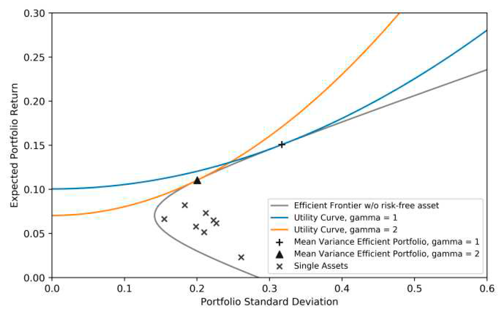
Figure 2.
Risk-return diagram depicting the minimum variance portfolio.
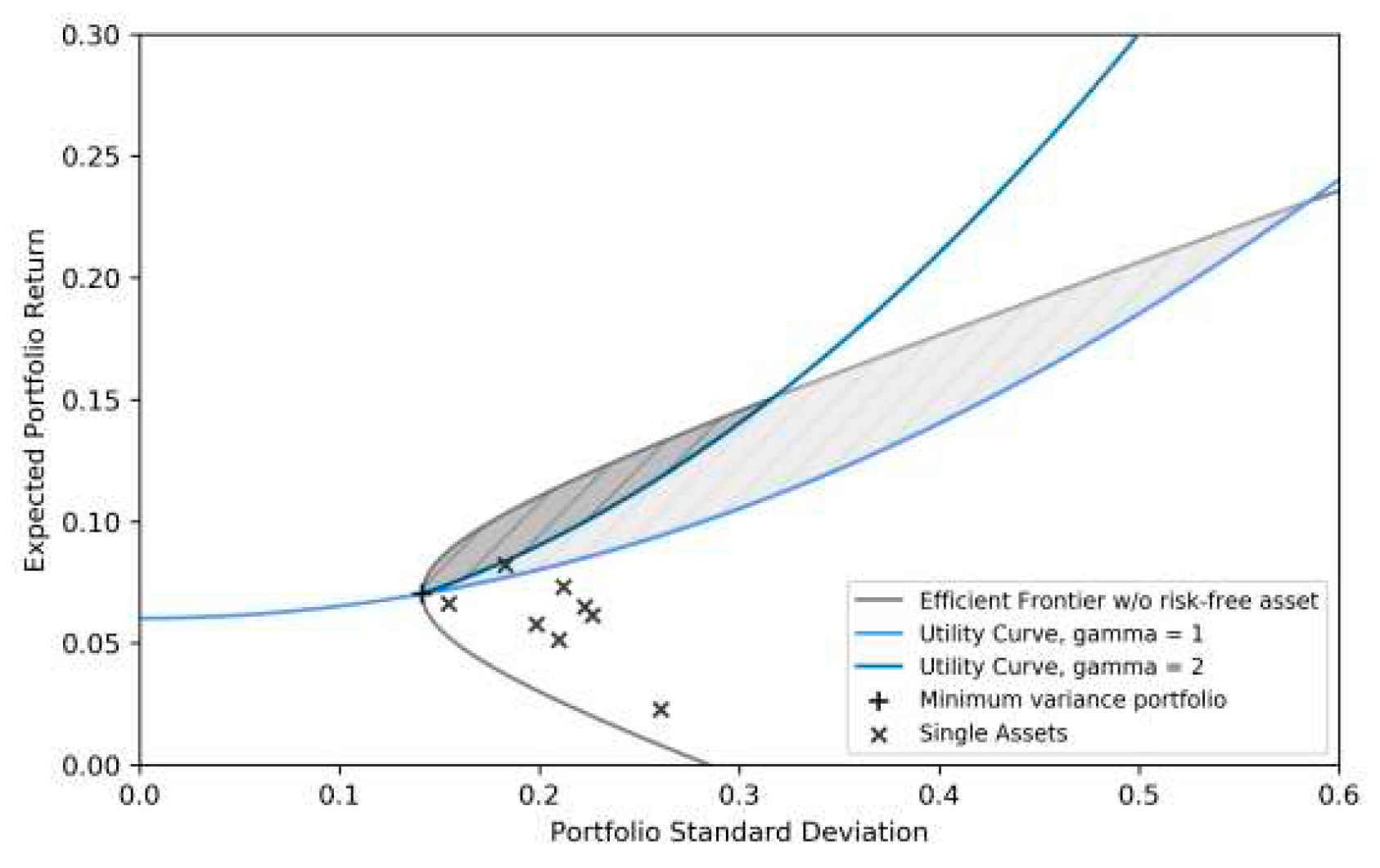
Figure 3.
Risk-return diagram of two-fund combinations.
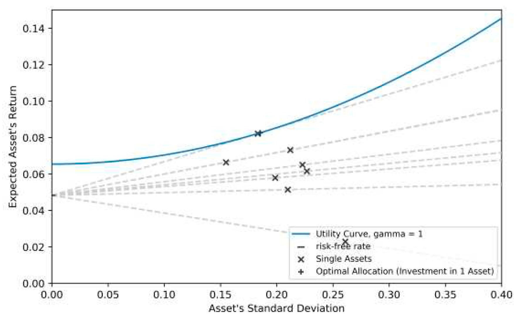
Figure 4.
Risk-return diagram including capital allocation line .
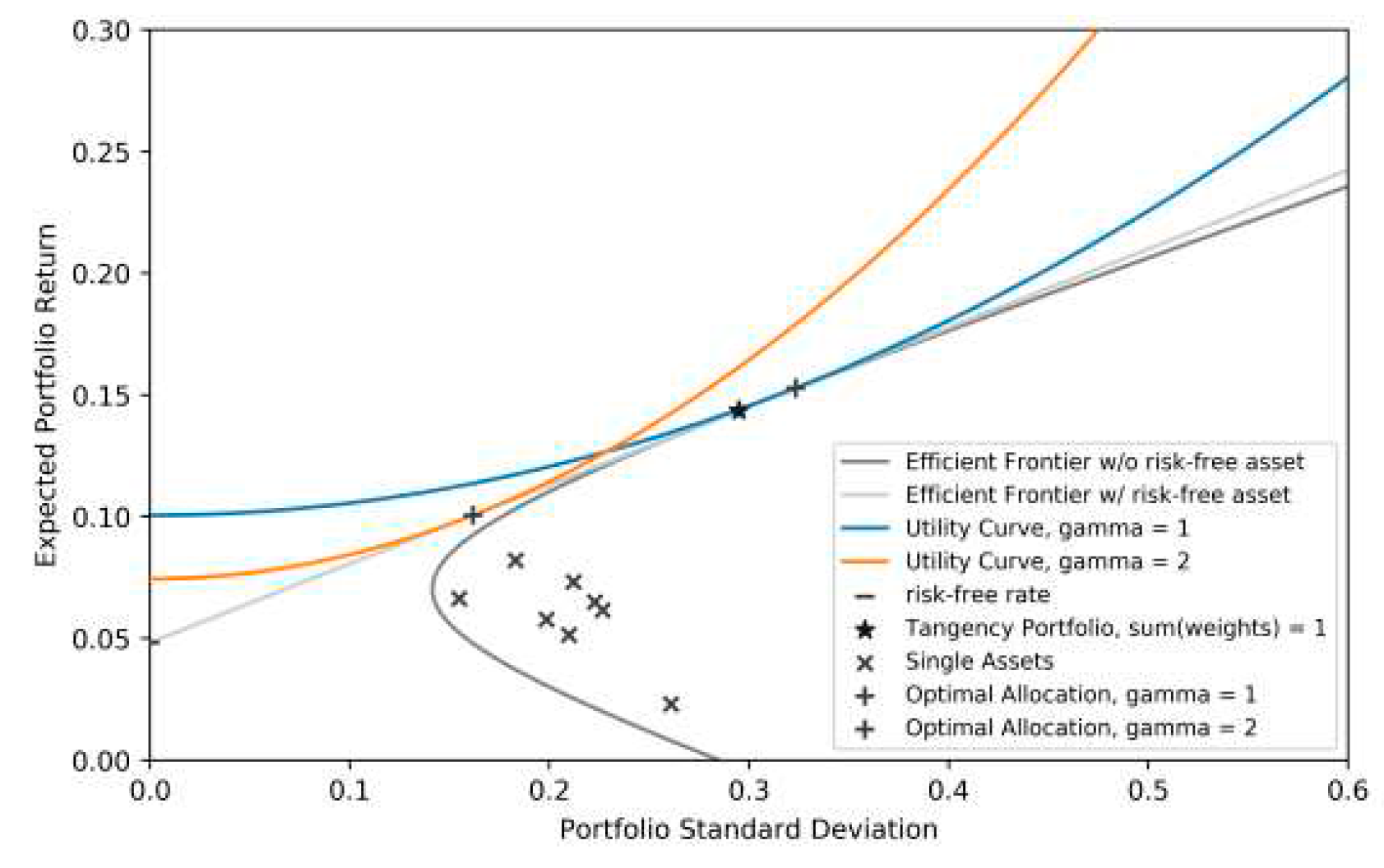
Figure 5.
Annualized risk-free yield.
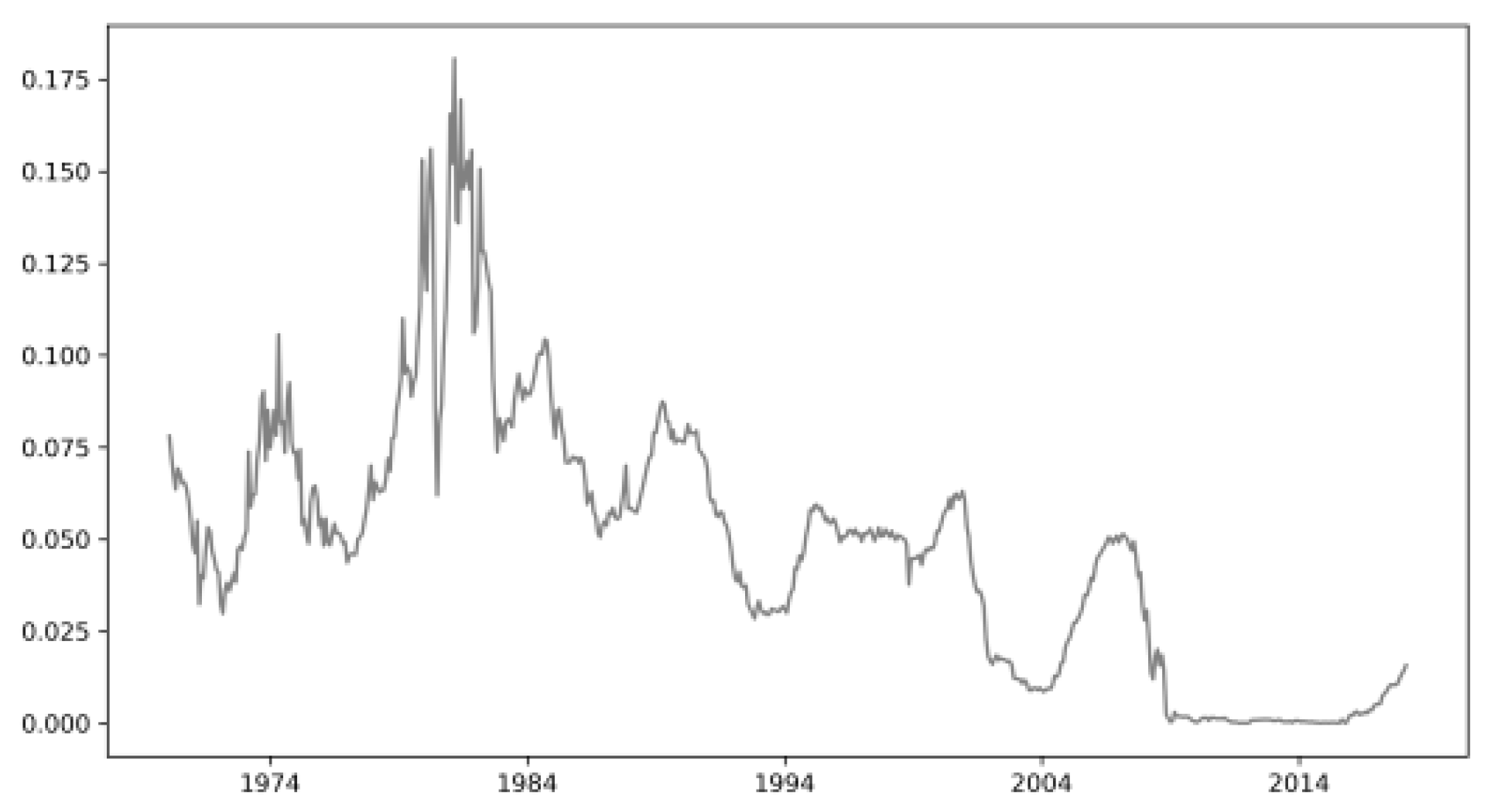
Figure 6.
Illustration of first estimation window and out-of-sample window.
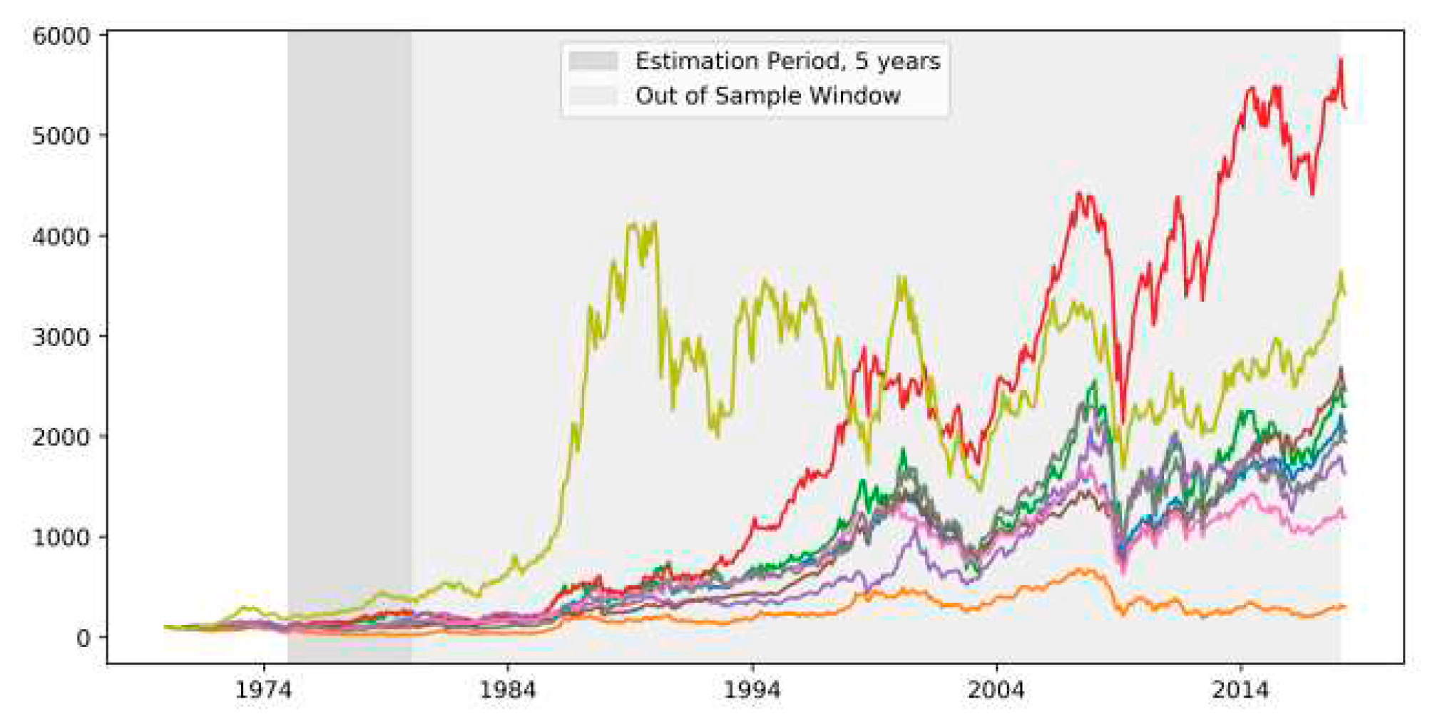
Figure 7.
Expected CER; = 1; short sale allowed
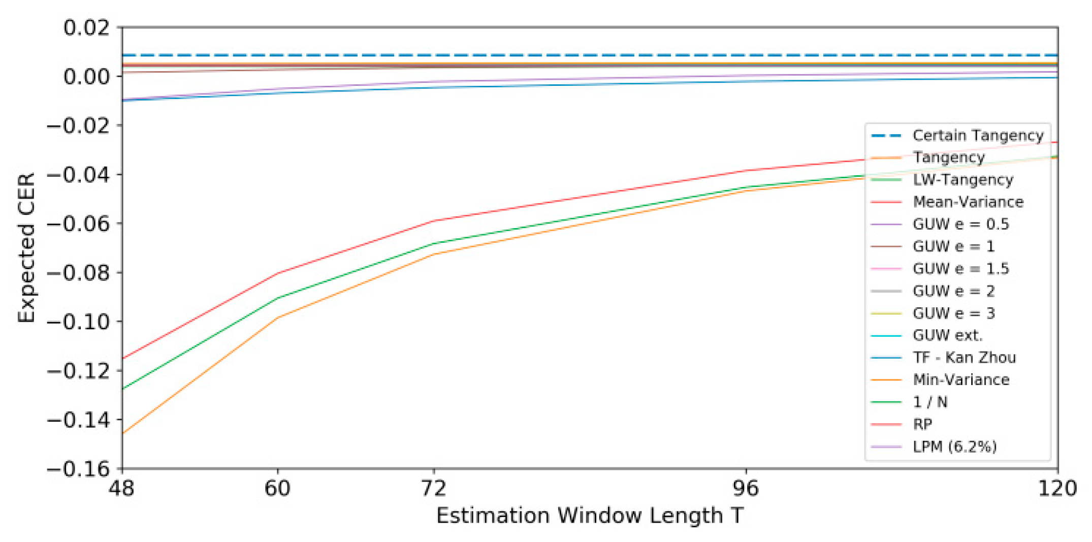
Figure 8.
Expected CER; = 1; short sale not allowed.
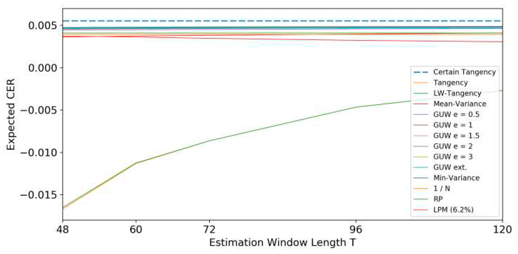

Table 1.
Annualized -vector and matrix of eight assets chosen.
|
annualized |
Variance-covariance matrix of annualized returns Σ | ||||||||
|---|---|---|---|---|---|---|---|---|---|
| Asset 1 | Asset 2 | Asset 3 | Asset 4 | Asset 5 | Asset 6 | Asset 7 | Asset 8 | ||
| Asset 1 | 2.30% | 6.81% | 3.03% | 2.36% | 2.32% | 1.79% | 2.71% | 3.60% | 2.02% |
| Asset 2 | 6.50% | 3.03% | 4.96% | 2.96% | 2.41% | 2.04% | 2.70% | 3.72% | 1.99% |
| Asset 3 | 8.22% | 2.36% | 2.96% | 3.35% | 2.01% | 1.75% | 2.44% | 2.88% | 1.85% |
| Asset 4 | 5.79% | 2.32% | 2.41% | 2.01% | 3.94% | 2.30% | 2.52% | 2.56% | 1.59% |
| Asset 5 | 6.64% | 1.79% | 2.04% | 1.75% | 2.30% | 2.40% | 2.10% | 2.10% | 1.21% |
| Asset 6 | 5.14% | 2.71% | 2.70% | 2.44% | 2.52% | 2.10% | 4.40% | 3.07% | 1.92% |
| Asset 7 | 6.15% | 3.60% | 3.72% | 2.88% | 2.56% | 2.10% | 3.07% | 5.14% | 2.13% |
| Asset 8 | 7.32% | 2.02% | 1.99% | 1.85% | 1.59% | 1.21% | 1.92% | 2.13% | 4.50% |
Table 2.
Asset allocation in a one-fund setting.
| Asset i | 1 | 2 | 3 | 4 | 5 | 6 | 7 | 8 |
|---|---|---|---|---|---|---|---|---|
| -92.35% | -27.61% | 173.13% | -32.26% | 96.97% - | 75.67% | 12.57% | 45.22% | |
| -43.50% | -15.75% | 97.92% | -17.70% | 82.01% - | -38.93% | 1.91% | 33.83% |
Table 3.
Portfolio characteristics in a one-fund setting.
| = 1 | = 2 | |
|---|---|---|
| 15.07% | 11.05% | |
| 31.71% | 20.04% |
Table 4.
Minimum variance portfolio weights.
| Asset i | 1 | 2 | 3 | 4 | 5 | 6 | 7 | 8 |
|---|---|---|---|---|---|---|---|---|
| 5.35% | -3.90% | 22.72% | -2.74% | 67.05% - | -2.19% | -8.74% | 22.74% |
Table 5.
Tangency portfolio weights .
| Asset i | 1 | 2 | 3 | 4 | 5 | 6 | 7 | 8 |
|---|---|---|---|---|---|---|---|---|
| -83.74% | -25.52% | 159.87% | -29.66% | 94.34% - | -69.19% | 10.69% | 43.22% |
Table 6.
Optimal two-fund allocation for = 1, 2.
| = 1 | = 2 | |
|---|---|---|
| 109.66% | 54.83% | |
| 15.29% | 10.06% | |
| 32.34% | 16.17% |
Table 7.
Indices considered for analysis.
| Countries | Ticker | Abbreviation | Currency |
|---|---|---|---|
| Italy | MSITALL | ITA | EUR (ITL) |
| Germany | MSGERML | GER | EUR (DEM) |
| Switzerland | MSSWITL | SWI | CHF |
| Canada | MSCNDAL | CAN | CAD |
| USA | MSUSAML | USA | USD |
| UK | MSUTDKL | UK | GBP |
| France | MSFRNCL | FRA | EUR (FF) |
| Japan | MSJPANL | JPN | JPY |
| World | MSWRLD | WRLD | USD |
Table 8.
Summary statistics of return series data used.
| Asset | Min | Max | Skew | Kurtosis | ||
|---|---|---|---|---|---|---|
| ITA | 0.191% | 7.53% | -52..91% | 26.39% | -0.68 | 4.57 |
| GER | 0.542% | 6.43% | -24.92% | 29.67% | -0.44 | 2.02 |
| SWI | 0.685% | 5.28% | -19.14% | 23.31% | -0.36 | 1.73 |
| CAN | 0.482% | 5.73% | -30.05% | 20.72% | -0.78 | 3.19 |
| USA | 0.553% | 4.47% | -24.36% | 16.17% | -0.71 | 2.95 |
| UK | 0.429% | 6.06% | -24.09% | 44.01% | 0.35 | 5.47 |
| FRA | 0.513% | 6.54% | -31.35% | 22.05% | -0.55 | 1.83 |
| JPN | 0.610% | 6.12% | -28.11% | 22.20% | -0.02 | 1.28 |
| WRLD | 0.521% | 4.37% | -20.84% | 14.14% | -0.70 | 2.29 |
Table 9.
Shapiro-Wilk test statistics and p-values; main data set.
| Asset | W | p-value | Reject |
|---|---|---|---|
| ITA | 0.96 | 1.3E-10 | YES |
| GER | 0.97 | 2.8E-09 | YES |
| SWI | 0.97 | 6.7E-09 | YES |
| CAN | 0.96 | 4.2E-12 | YES |
| USA | 0.96 | 5.8E-11 | YES |
| UK | 0.95 | 1.2E-12 | YES |
| FRA | 0.98 | 4.7E-08 | YES |
| JPN | 0.99 | 2.8E-04 | YES |
| WRLD | 0.9625 | 5.4E-11 | YES |
| All Assets | 0.9661 | 2.5E-33 | YES |
Table 10.
and ; annualized figures.
| Asset | ITA | GER | SWI | CAN | USA | UK | FRA | JPN | WRLD |
|---|---|---|---|---|---|---|---|---|---|
| ITA | 6.81% | 3.03% | 2.36% | 2.32% | 1.79% | 2.71% | 3.60% | 2.02% | 2.29% |
| GER | 3.03% | 4.96% | 2.96% | 2.41% | 2.04% | 2.70% | 3.72% | 1.99% | 2.45% |
| SWI | 2.36% | 2.96% | 3.35% | 2.01% | 1.75% | 2.44% | 2.88% | 1.85% | 2.07% |
| CAN | 2.32% | 2.41% | 2.01% | 3.94% | 2.30% | 2.52% | 2.56% | 1.59% | 2.32% |
| USA | 1.79% | 2.04% | 1.75% | 2.30% | 2.40% | 2.10% | 2.10% | 1.21% | 2.08% |
| UK | 2.71% | 2.70% | 2.44% | 2.52% | 2.10% | 4.40% | 3.07% | 1.92% | 2.44% |
| FRA | 3.60% | 3.72% | 2.88% | 2.56% | 2.10% | 3.07% | 5.14% | 2.13% | 2.54% |
| JPN | 2.02% | 1.99% | 1.85% | 1.59% | 1.21% | 1.92% | 2.13% | 4.50% | 2.14% |
| WRLD | 2.29% | 2.45% | 2.07% | 2.32% | 2.08% | 2.44% | 2.54% | 2.14% | 2.29% |
| 2.30% | 6.50% | 8.22% | 5.79% | 6.64% | 5.14% | 6.15% | 7.32% | 6.25% |
Table 11.
Expected monthly CER = 1; short sale allowed.
| Estimation window length T | |||||
|---|---|---|---|---|---|
| Utility-Optimized Portolios | 48 | 60 | 72 | 96 | 120 |
| Certain Tangency | 0.855% | 0.855% | 0.855% | 0.855% | 0.855% |
| Tangency | -14.603% | -9.856% | -7.274% | -4.690% | -3.334% |
| LW-Tangency | -12.776% | -9.056% | -6.835% | -4.540% | -3.271% |
| Mean-Variance | -11.542% | -8.047% | -5.912% | -3.863% | -2.691% |
| = 0.5 | -0.966% | -0.528% | -0.233% | 0.016% | 0.016% |
| = 1 | 0.137% | 0.251% | 0.336% | 0.401% | 0.443% |
| = 1.5 | 0.397% | 0.434% | 0.466% | 0.491% | 0.508% |
| = 2 | 0.462% | 0.482% | 0.500% | 0.515% | 0.526% |
| = 3 | 0.493% | 0.504% | 0.517% | 0.526% | 0.534% |
| GUW ext. | 0.433% | 0.438% | 0.452% | 0.457% | 0.466% |
| TF - Kan Zhou | -1.016% | -0.704% | -0.475% | -0.227% | -0.064% |
| Benchmark Portfolios | |||||
| Min-Variance | 0.492% | 0.496% | 0.500% | 0.501% | 0.502% |
| 1 / N | 0.393% | 0.393% | 0.393% | 0.393% | 0.393% |
| RP | 0.408% | 0.408% | 0.409% | 0.409% | 0.409% |
| LPM (6.2%) | 0.436% | 0.434% | 0.430% | 0.430% | 0.402% |
Table 12.
Expected monthly CER = 1; no short sale.
| . | Estimation window length T | ||||
|---|---|---|---|---|---|
| Utility-Optimized Portolios | 48 | 60 | 72 | 96 | 120 |
| Certain Tangency | 0.555% | 0.555% | 0.555% | 0.555% | 0.555% |
| Tangency | -1.670% | -1.132% | -0.865% | -0.466% | -0.271% |
| LW-Tangency | -1.652% | -1.126% | -0.864% | -0.467% | -0.271% |
| Mean-Variance | 0.361% | 0.374% | 0.381% | 0.397% | 0.410% |
| = 0.5 | 0.5 0.444% | 0.448% | 0.452% | 0.457% | 0.462% |
| = 1 | 1 0.457% | 0.460% | 0.463% | 0.469% | 0.473% |
| = 1.5 | 1.5 0.463% | 0.466% | 0.470% | 0.474% | 0.478% |
| = 2 | 2 0.466% | 0.470% | 0.473% | 0.478% | 0.482% |
| = 3 | 3 0.471% | 0.474% | 0.478% | 0.482% | 0.485% |
| GUW ext. | 0.462% | 0.464% | 0.466% | 0.469% | 0.472% |
| TF - Kan Zhou | - | - | - | - | - |
| Benchmark Portfolios | |||||
| Min-Variance | 0.474% | 0.478% | 0.481% | 0.485% | 0.487% |
| 1 / N | 0.393% | 0.393% | 0.393% | 0.393% | 0.393% |
| RP | 0.408% | 0.408% | 0.408% | 0.408% | 0.408% |
| LPM (6.2%) | 0.372% | 0.362% | 0.346% | 0.323% | 0.306% |
Table 13.
Expected monthly CER varying ; ; short sale allowed.
| Risk aversion coefficient γ | |||||
|---|---|---|---|---|---|
| Utility-Optimized Portolios | 0.5 | 1.0 | 1.5 | 2.0 | 3.0 |
| Certain Tangency | 1.320% | 0.855% | 0.700% | 0.622% | 0.545% |
| Tangency | -20.102% | -9.856% | -6.441% | -4.733% | -2.165% |
| LW-Tangency | -18.501% | -9.056% | -5.907% | -4.333% | -2.019% |
| Mean-Variance | -16.552% | -8.047% | -5.247% | -3.871% | -1.823% |
| = 0.5 | -1.339% | -0.528% | -0.307% | -0.230% | -0.074% |
| = 1 | 0.203% | 0.251% | 0.219% | 0.174% | 0.136% |
| = 1.5 | 0.518% | 0.434% | 0.361% | 0.295% | 0.213% |
| = 2 | 0.564% | 0.482% | 0.409% | 0.343% | 0.249% |
| = 3 | 0.573% | 0.504% | 0.440% | 0.378% | 0.281% |
| GUW ext. | 0.533% | 0.438% | 0.360% | 0.291% | 0.192% |
| TF - Kan Zhou | -1.798% | -0.704% | -0.340% | -0.158% | 0.025% |
| Benchmark Portfolios | |||||
| Min-Variance | 0.543% | 0.496% | 0.449% | 0.402% | 0.315% |
| 1 / N | 0.448% | 0.393% | 0.339% | 0.284% | 0.175% |
| RP | 0.461% | 0.408% | 0.356% | 0.304% | 0.199% |
| LPM (6.2%) | 0.500% | 0.434% | 0.367% | 0.300% | 0.166% |
Disclaimer/Publisher’s Note: The statements, opinions and data contained in all publications are solely those of the individual author(s) and contributor(s) and not of MDPI and/or the editor(s). MDPI and/or the editor(s) disclaim responsibility for any injury to people or property resulting from any ideas, methods, instructions or products referred to in the content. |
© 2023 by the authors. Licensee MDPI, Basel, Switzerland. This article is an open access article distributed under the terms and conditions of the Creative Commons Attribution (CC BY) license (http://creativecommons.org/licenses/by/4.0/).
Copyright: This open access article is published under a Creative Commons CC BY 4.0 license, which permit the free download, distribution, and reuse, provided that the author and preprint are cited in any reuse.


