Submitted:
28 November 2023
Posted:
29 November 2023
You are already at the latest version
Abstract
The CMT (Cold Metal Transfer) arc welding process is a convenient instrument for the assembly of thin sheets [1], [2]. More particularly, it permits the decrease of the amount of heat transferred to the parts to-be assembled, thus reducing their subsequent deformations.
The present work aims at simulating the CMT welding of thin stainless-steel sheets in order to develop an approach that allows the prediction of temperature fields, as well as final deformations induced by the welding process. For that purpose, instrumented tests and numerical simulations were set aiming at comparing the experiments with simulations.
Butt-welding of stainless-steel sheets was considered, with a thickness ranging from 1 to 1.2 mm. The weld seam samples were observed in order to set an equivalent heat source for each configuration. Moreover, the electric current and voltage were surveyed, and temperature measurements were performed using K-type thermocouples. In addition, displacement measurements were obtained using the DIC (Digital Image Correlation) technique.
Thermomechanical simulations were then carried out using an equivalent heat source approach, considering the phase changes of elements, i.e. the transitions from solid to liquid and from liquid to solid. These simulations also consider the actual geometry of seams induced by addition of a filler material.
Keywords:
CMT process
; welding automation
; sheet metal
; austenitic stainless-steel
; Numerical simulation
1. Introduction
The present study aims at limiting the weight of welded steel structures in the context of road transport. One way consists in decreasing the thickness of the sheets, and avoiding any stiffness loss, by applying other means.
Welding operations give rise to deformations and internal stresses that could compromise the durability of the structure. For the sake of balancing the probable stiffness loss, alternative techniques, including reinforcement in the manufacturing of structures, are put forward by the company Magyar. Moreover, numerical simulation of the metal structure assembling process can be conducted in order to forecast the temperature fields and deformations caused by the welding process.
As part of this project, a thermomechanical simulation was performed for the MAG (Metal Active Gas) / CMT (Cold Metal Transfer) welding process applied to structures constructed from thin-walled austenitic stainless-steel sheets. In this context, a comprehensive program of tests and numerical simulations has been outlined, which would permit comparisons between the conducted experiments and corresponding simulations. More specifically, the observation encompasses both the thermal and mechanical phenomena that occur during welding operations.
The experimental aspect of this study focuses on instrumented welding tests that involve sheets with a thickness ranging from 1 to 1.2 mm. This instrumentation primarily encompasses thermal measurements using thermocouples (TC), measurements of welding current and voltage, and acquisition of displacement data to assess sheet deformations through Digital Image Correlation (DIC) technique. Furthermore, macrograph samples of the weld seams are observed to identify and to model the equivalent heat source for welding conditions of 304L stainless-steel grade. The process for establishing these analogous sources is based on experimental measurements of the dimensions and properties of Molten Zones (MZ), followed by recalibrating the geometric and energy parameters of a pre-set heat source. The provided equivalent heat sources are then incorporated into thermomechanical calculations.
Modeling and simulation of thermal and thermomechanical behaviors were conducted using the ABAQUS commercial computation software, employing sub-programs (DFLUX) coded in FORTRAN to incorporate the thermal sources required by this approach.
For these experiments, the CMT welding process introduced by Fronius in 2004 [3] was selected. This process involves the assistance of a mechanical recoil of the wire to facilitate the detachment of the metal droplet. The welding operation is synchronized to ensure the detachment and deposition of the droplet that occurs when the current reaches almost zero (when the electrical resistance R is high), [4].
Several references highlight the advantages of the CMT process, particularly in the context of thin sheets joining [5,6]. In a study conducted by Talalaev et al. [6], the authors discuss the problem of distortion and deformation of stainless steel parts with a thickness ranging from 2 to 4 mm during welding. They have demonstrated that a welding velocity Vw in the range of 600-720 mm/min ensures low porosity and minimizes the product distortion. The authors also suggested that optimization of heat input Q between 70 and 110 J/mm, ensures adequate joint penetration while minimizing deformations.
Gas-shielded welding, particularly the CMT process, is highly valuable in industries like automotive, aeronautics, aerospace, and metal production. CMT offers an innovative arc-welding approach suitable for automation. It maintains lower temperatures, enabling the welding of thin metal sheets in an edge-to-edge configuration, but for thicknesses that are not less than 0.3 mm. Key features of the CMT process include a controlled short arc interruption and wire movement integration, resulting in uniform, spatter-free welding. At frequencies up to 70 Hz, short-circuits occur automatically, reducing current and heat. Compared to traditional MIG (Metal Inert Gas) (/MAG welding, CMT offers lower heat input and a stable arc. It is ideal for thin materials, causing minimal damages to the base metal, expanding tolerance ranges, and providing clean welding in any position or speed [7].
2. Experimental conditions
In the current study, a number of butt-welding tests have been carried out on samples with a thickness ranging from 1 to 1.5 mm. They are composed of two 100 mm x 80 mm stainless steel sheets. These configurations (including variations of the thicknesses) were selected to account for the variability of the bottom and shell thicknesses to be welded for the construction of tanks. All MIG/CMT welding experiments have been carried out with a FRONIUS CMT 4000 welding generator.
The first specimen consisted of two sheets of equal thicknesses (1 mm), while the second specimen involved two sheets with different thicknesses, specifically 1.2 mm and 1 mm. To minimize deformation, these two sheets were welded in contact with a copper lath in order to avoid any overheating of the base metal.
Welded sheets were equipped with instrumentation, allowing for the measurement of temperatures both during and after welding. Temperature measurements were performed as close as possible from the weld line, and achieved by fixing K-type thermocouples in the vicinity of the welding area. To safeguard these thermocouples from heat damage during welding, they were shielded by small metal sheets, Figure 1.
These two thermocouples (TC0 and TC1) were positioned at the center of the sheet, with a 20 mm gap regarding to the welding line, as illustrated in Figure 1. This distance ensures that the thermocouples are not exposed to burning during welding, a situation typically encountered in CMT welding, where the width of the weld seam is more substantial compared to other processes such as TIG (Tungsten Inert Gas) welding.
Clampings were positioned on both sides of the sheet, extending all the way to the ends in both the transverse and longitudinal directions of the sheet, with a 30 mm gap from the weld line. This clamping setup guarantees that both sides of the sheet remain firmly in place during the welding process.
To prevent any misalignment during CMT welding, both coupons were initially Laser spot welded each 25 mm before CMT welding. In addition, LASER technology was used to minimize distortion resulting from this pointing process.
During the CMT processing, a welding speed of 650 mm/min was selected, which is consistent with Talalaev’s suggestions [6].
Displacements and deformations caused by welding were measured using the DIC technique [8]. This measurement method involves applying a speckle pattern to the sheet surface before welding. The speckle pattern consists of a white background with random black spots of varying sizes. DIC measurements are executed using VIC3D software.
Figure 1 illustrates the welding process with a copper lath, application of the speckle pattern on metal sheets, thermocouples protected by small metal sheets, and clamping conditions employed during welding experiments. The clamping was maintained during the cooling phase.
Measuring the electric current and voltage values allows to get a more accurate estimation of the power dissipated within the primary welding circuit.
Indeed, it is important to note that the desired voltage and current parameters may not always be achieved during an arc welding experiment. Various events may transpire during the test, such as short circuits or oscillations of the bath surface, that may result in an operating point that the generator cannot attain, or a change in the transfer mode. All that can lead to alterations in voltage and/or current values.
In electric arc welding, linear welding energy is a function of welding speed, and effective arc voltage and current. It is expressed as follows:
With: U arc voltage (V); I arc current intensity (A); and Vw (mm/min) to provide (kJ/mm).
Determining the welding speed is a straightforward process. When it comes to voltage (U) and current (I), we typically rely on values obtained by averaging several measurements. These measurements can be taken directly from the welding generator if it undergoes periodic checks, or from calibrated external devices. In our studies, current clamps are used to measure I(t) and U(t), displaying the actual (effective) current and voltage (Ieff and Ueff), as demonstrated in Figure 2.
These devices allow capturing U(t) and I(t) with a high acquisition frequency, digitally multiplying the two to derive an instantaneous power value P. This value can be averaged over a specific duration, or it can be used to calculate the total energy , making the determination of welding energy quite straightforward.
The Effective Current or voltage represents the value of direct current or voltage that yields the same power dissipation due to the Joule effect in a resistive circuit.
With: Es: welding energy (kJ/mm);
P: Average power (kW);
: arc-on time (s);
L: weld length (mm);
: cumulative energy (kJ).
Voltage and current measurements were thus monitored during the welding process, and these measurements provided curves depicted in Figure 2. For voltage monitoring, a differential probe was used, specifically the MX9030 by Chauvin-Arnoux. This probe was connected to the welding circuit, with a measurement location carefully selected to be as close to the welding arc as possible. One connector was affixed to the conductor guide positioned between the torch pusher roller and the contact tube, while the other connector was attached to the generator ground cable.
A Chauvin-Arnoux PAC 21 current clamp was used to monitor the welding current. This PAC 21 clamp was positioned on the ground cable and operated based on the Hall effect principle. The acquisition of voltage and current signals was carried out using a National Instrument CompactRIO system. Our data collection encompassed a total of 60,000 measurement points, with an acquisition time of 60 seconds and a sampling period of 0.001 seconds.
The primary contributors to the induced heat cycle, are the energy effectively conveyed to the workpiece and the initial temperature, and these factors take precedence regardless of the material physical characteristics.
Nevertheless, owing to several forms of dissipation, including radiation, convection, and conduction losses, the energy furnished by the electric arc is never entirely transferred to the workpiece. Consequently, not all of the thermal energy is transferred to the workpiece during the welding process, as a portion of it is lost through conduction within the wire guides and wire sheaths.
The calculation of heat input, denoted as , can be expressed as:
: Process thermal efficiency coefficient, considered as 0.8 for the CMT process.
The use of an amperemeter for measuring current intensity and a voltmeter for voltage allowed us to determine the effective welding energy transferred to the workpiece over a specific duration, as demonstrated in the example Figure 2. Additionally, these measurements facilitated the estimation of the heat input and the actual average power absorbed by the sheets in various butt configurations, such as the 1 mm / 1 mm and 1.2 mm / 1 mm configurations, as detailed in Table 1.
Figure 3 presents the macroscopic cross-sectional views achieved through the process for butt-end configurations. It provides an overview of the macrographs for the two test cases. It is evident that both welding conditions exhibit complete penetration. Furthermore, it is noticeable that the heat input required to melt the base metal in these two tests is nearly identical. Specifically, since both tests involve a 1 mm thickness on one side, the welding parameters are consistent, ranging from 0.188 kJ/mm to 0.196 kJ/mm. This translates to a negligible relative difference of less than 3%.
However, it can also be seen that the use of almost identical welding parameters has resulted in two different seam geometries: the lower joint surfaces have a smaller radius of curvature due to the greater thermal pumping (contact with the copper lath), and the MZ surface of the 1 mm / 1 mm configuration is larger than that of the 1.2 mm / 1 mm configuration, due to the quality of the contact with the copper lath.
Figure 4 and Table 2 depict the schematic and average numerical values of the macrographic measurements for the weld seam dimensions in the context of these two tests. It is worth noting that, in addition to penetration and width, there are several other dimensions to consider in the cross-section of the joint. h, H, l, L, and e represent distinct weld seam dimensions, whereas e1 and e2 are the sheet thicknesses.
Maximum depth difference (e) of the MZ between the two configurations amounts to 0.1 mm. In the 1 mm / 1 mm case, both the upper (L) and lower (l) widths of the melted zone are slightly greater than those observed in the 1.2 mm / 1 mm configuration. This difference can be explained by a slight, non-significant difference in the average real power absorbed for the two configurations.
3. Numerical model
In order to establish a comparison between simulations and experiments, this section presents the numerical model used to simulate actual welding experiments using the Finite Element Method (FEM), and taking into account initial and boundary conditions. Corresponding thermomechanical calculations using an equivalent heat source approach were then performed.
Simulation results obtained using this approach allows determining the evolution of temperature during welding, as well as to evaluate the deformations and angles of the sheets distortion resulting from the welding operations.
The "heat source identification" and "thermomechanical calculations" sections are based on numerical simulation and experimentations. The equivalent heat sources were identified for both selected end-to-end configurations.
The calculation of deformations requires identification of a behavior law for both the base material and the molten zone. These laws were obtained from the literature, [9,10,11].
In the chosen approach, the stages of numerical simulation of welding involve, firstly, using the geometric and energy parameters to identify an equivalent heat source for each configuration. Secondly, simulated temperature fields during heating and cooling are compared to those obtained experimentally. The next step is to determine the displacements/deformations of the metal sheets from the thermomechanical calculations.
The Finite Element (FE) mesh size was chosen on the basis of literature comparable to our study [12,13,14,15]. In order to reduce calculation times, the mesh was defined including two transition zones 1 and 2 along the transverse direction. To optimize calculation time and accuracy, the size of elements is finer in and around the MZ and HAZ (Heat Affected Zone). On the other hand, elements become coarser away from the weld zone. In the direction of the weld axis, the mesh size is a constant 0.25 mm.
In the weld zone, eight elements are used across the sheet thickness, providing an element size of 0.125 mm. These eight elements become four when separated from the weld in the transverse direction, and the change is operated through a first transition zone (label 1). Similarly, the four elements go through a second transition (label 2) to become two elements.
Thus, the mesh becomes coarser between zone 1 and 2 based on the progressive refinement along the lateral lines outside the weld seam. The minimum mesh size is 0.125 mm and the maximum 0.5 mm.
The FE model, including two transition zones and a progressive refinement along the lateral lines, is shown in Figure 5, it is inspired by literature [16] and [17].
The use of these transition zones allowed reducing the number of elements, nodes and total CPU time for each configuration, as detailed in Table 3.
An isostatism condition was considered for the mechanical boundary conditions and C3D8RT elements were used as suggested in the literature review [14,18,19]. This type of element (3D bricks with eight nodes) is suitable for thermomechanical calculations.
Within ABAQUS, the steps used in the present study are divided into three groups, the first group of steps is used to apply initial conditions and clamping, and consists of two steps, the second group is used to simulate progressive activation of elements, and the number of steps corresponds to the number of elements, e.g. 25 steps for 25 elements, the last group is used for debriding and cooling, and consists of a single step. Thermomechanical properties (Poisson's ratio, Young's modulus, yield strength, density, specific heat, thermal conductivity, latent heat of fusion, solidus and liquidus temperatures) as a function of temperature, were taken from the literature [17,20,21].
Several values of the heat exchange coefficient h were applied to investigate its effect on the maximum predicted temperature. An adjustment of the heat exchange coefficient was hence done in order to provide the best fit between experimental and calculated temperatures. Finally, the selected coefficient h takes into account both convection and radiative contributions.
For this, values of h, ranging between 10 and 60 W.m-2.°C-1 were tested. The choice of welding on a copper lath was made in view of the very low thickness of the sheets to be welded. It is essential to avoid any risk that the weld pool collapses when assembling this type of sheet. Copper was also chosen because it cools the weld pool very quickly, thus avoiding oxidation problems on the reverse side of the weld seam.
A Bilinear Isotropic Strain Hardening Model was selected to set up the elastoplastic behavior. This type of model allows considering the dependence of properties (Young’s modulus 𝐸, Tangent modulus 𝐸𝑡 and Yield stress 𝜎𝑒) on temperature. The Plastic strain 𝜀𝑝𝑙 was determined from literature data [19] obtained from experimental nominal stress-nominal strain curves, Figure 6.
This type of behavior law includes three material parameters that are necessary for the calculation: 𝐸, 𝐸𝑡 and 𝜎𝑒. The strain-hardening parameter µ represents the ratio between the 𝐸𝑡 and the 𝐸.
A sensitivity study was carried out by Akbari Mousavi [9], and Brickstad [10] in order to determine the value of µ for 304L and 316L stainless steels at different temperatures , and to assess the influence of varying this value on the obtained final deformation. Finally, the µ ratio was set to 0.0133 for temperatures up to 800°C, and to 0.0001 above 800°C.
In the present work, the elastoplastic behavior model of 316L stainless-steel was assumed to be identical to that of 304L, since Young's moduli as a function of temperature are almost identical [16,17,22].
In ABAQUS software, thermal strains are determined by the following mathematical formula:
With:
: Thermal strain;
: Average coefficient of thermal expansion at a current temperature (°C-1);
: Current temperature (°C);
: Average coefficient of thermal expansion at an initial temperature (°C-1);
: Initial temperature (°C);
: Metal reference temperature (°C).
The reference temperatures for the base metal and seam metal used in our calculations are 25°C (ambient temperature) and 1450°C (melting temperature) respectively.
The ABAQUS "NLGEOM" parameter was used to activate the large deformations option since the small deformation option was found to provide non-realistic results.
Residual deformations induced by the sheet manufacturing process, e.g. rolling, were not taken into account. It was assumed that, at the melting point of the material, local plastic deformation are suppressed and new plastic deformation is prevented after melting (i.e. the transition from liquid to solid state), so that the material is reconstructed and the history of the material is assumed to be erased locally under the effect of previous treatments [23].
It was assumed that the weld seam is divided into several elements of equal length, which were activated progressively during welding.
This was simulated using the "Element Birth and Death" technique available within ABAQUS and well explained in [24,25,26]. The elements are considered inactive at the beginning of welding process, i.e. "dead" at the start of the calculation. They are then activated as the heat source progresses, i.e. “births". This technique is adopted to simulate a real welding process, as the seam is formed by a mixture of base metal and filler metal. A quantity of filler metal material is deposited evenly as the filler wire melts. The filler metal is modeled by the progressive activation of elements of a previously meshed seam. This approach assumes that the geometry of the seam is known before the calculation is carried out (geometry of the equivalent heat source, Figure 4 and Table 2).
An equivalent heat source approach was adopted, with an imposed cross-section propagated along a length Lw in the direction of the seam axis. The cross-section is made up of two disc-segments separated by an intermediate trapezoid: it is therefore a prismatic type source. The elements are progressively activated during calculations, and the source is moving linearly in time: an example is shown in Figure 7. Note that Lw represents the optimum value for element length, for which calculation results close to reality have been obtained.
This source was used to represent the distribution of absorbed energy across the thickness of the sheets. Temperature fields were calculated taking into account thermal convection effects. The initial temperature of the sheets was 25°C, and an overall heat exchange coefficient was taken into account, as elaborated earlier. Finally, the coupling between the thermal problem, and the mechanical one is weak.
This approach, which enables the shape of the molten zone to be represented, was implemented in a DFLUX subroutine coded in FORTRAN. It takes the history of elements into account, which means changes from solid to liquid state, and liquid to solid. It also takes the actual geometry of the seams into account, which varies strongly with the filler material addition, as suggested on Figure 3.
A three-dimensional thermomechanical model was developed to calculate deformations for a suitable equivalent volumetric heat source. A welding speed of 0.65 m/min was considered, as well as the average real power input provided for each configuration (homogeneously distributed in the volume of the prismatic source as shown on Figure 7.
4. Results and discussions
This section presents the FE results of the thermal and mechanical simulations, applied to experiments described previously. A comparative analysis of thermal and mechanical results computed for each configuration is performed. In addition, temperature measurements and digital image correlation results are compared to the predicted temperatures and displacement fields. Finally, the measured deformation angles are compared to the predicted ones.
Comparison between the experimental macrostructure of the weld bead, and the predicted geometry of the MZ for the two different welding cases, is shown in Figure 8.
Table 4 summarizes the maximum temperatures recorded by TC0 and TC1 thermocouples on the assembly shown in Figure 1, i.e., thermocouples placed at 20 mm from the weld seam. The maximal temperatures recorded do not exceed 260°C for the 1 mm / 1 mm configuration, and 340°C for the 1.2 m / 1 mm configuration, due to the increase of the conductive thermal resistance between the TC measurement point and the copper lath. Temperatures then drop progressively to ambient temperature.
Despite the welding parameters being almost identical for the two configurations (power, wire feed rates, and welding speeds), when linearly approximating the heating and cooling phases on the graphs shown in Figure 9 and Figure 10, it is clear that the average heating and cooling rates for the 1 mm / 1 mm configuration (11 °C/s and 0.47 °C/s, respectively) exceed those for the 1.2 mm / 1 mm configuration (8.12 °C/s and 0.39 °C/s). This might be correlated to the higher cross-sectional area of the MZ in the former configuration (17.9 mm2) in comparison with the latter one (17 mm2).
In the context of 1 mm thick sheet metal sections, the maximum temperature achieved in the first configuration (1 mm / 1 mm) is lower than that recorded in the second configuration (1.2 mm / 1 mm): 254°C for the former compared to 272°C for the latter.
In the case of the second configuration, the peak temperature reached by the 1.2 mm sheet section exceeds that measured for the 1 mm sheet section, as depicted in Table 4 and Figure 10. These phenomena are likely linked to the presence of the copper lath: the conductive thermal resistance between the TC measurement point and the copper lath increases by 20% for the 1.2 mm / 1 mm configuration.
Figure 9 shows the results of the thermal parametric study for the 1 mm / 1 mm configuration. It demonstrates the transient temperature evolution during welding and cooling at a point located 20 mm from the seam axis on the upper surface of the sheet.
The relative difference between the maximum calculated temperatures and those measured in the two parts of the sheet once assembled (thickness 1 mm) is low, which confirms the good correlation, Table 5.
The maximum temperature calculated with a heat exchange coefficient h = 30 W.m-2.°C-1 provides a smaller relative difference compared to other values of the heat exchange coefficient (this difference is lower than 3%).
Comparison between experimental results and the computed ones, according to variable heat exchange coefficients chosen beforehand: h = 10, 20 and 30 W.m-2.°C-1, provided a satisfactory comparison for h = 30 W.m-2.°C-1, and higher differences for h = 10 and 20 W.m-2.°C-1.
Figure 10 exhibits the results of the thermal parametric study for the 1.2 mm / 1 mm configuration. It spots light on the temperature evolution during welding and cooling at a point located 20 mm from the seam axis and on the upper surface of the assembly, in both the 1.2 mm and 1 mm thick sheets.
A comparison between experimental results with the computed ones is indicated, based on the application of variable values of the h (chosen beforehand among h = 30, 45 and 60 W.m-2.°C-1). Again, the comparison yields to satisfactory conclusions for h = 30 W. m-2.°C-1, and higher differences for the two other values of h.
The relative difference between the maximum calculated temperature and the measured ones in the 1 mm thick section of the assembly gives results closer to reality (the difference is less than 13% for the three different values of h), Table 6. In the 1.2 mm thick section, the difference is less than 14% for h = 30 W.m-2.°C-1, and greater than this percentage for the other values of h. This can be explained by the loss of contact between the copper lath and the sheet during welding, due to induced deformation.
Finally, the heat transfer coefficient retained for both calculations is thus h = 30 W. m-2.°C-1. This coefficient is justified by the fact that CMT is performed on metal sheets in direct metallic contact with a copper lath, and also by the fact that it also includes radiation.
Using the equivalent heat source approach for the thermo-mechanical calculation enabled to make a comparison between computed results and experiments at the deformation level.
An example of the results of calculated displacements (U2 or V) in the Y direction, normal to the sheet surface, after welding, case 1 mm / 1 mm, is shown in Figure 11. The overall deformation may be observed, and estimates of the deformation angle of the sheet after cooling may be derived. The same type of overall deformation is observed in both cases: the assembly takes on a shape of horse saddle.
In order to measure the deformation angle at the sheet ends, extraction of the vertical displacement profile (V) was performed for two lines L0 along the sheet width direction (X), see Figure 11.
Figure 12 show the comparison between experiments (DIC measurements line L0) and simulations for the vertical displacements (V) along the width (line L0). Measurements and calculations show similar concave curvatures.
Comparison of the thermomechanical calculation results with experimental ones for the two cases yielded satisfactory conclusions for the cross-sectional direction of the sheet (80 mm), i.e., for the 1 mm / 1 mm case.
The calculated deformation angle is close to the real angle, which is around 2.7°, the difference between calculation and reality being around 0.3°. For the 1.2 mm / 1 mm case, the difference between calculation and reality is 0.1° for the 1 mm thick coupon and 0.3° for the 1.2 mm thick coupon, see Table 7.
Vertical displacement amplitudes and deformation angles at the ends of the thickest coupons are greater than those of thinner sheets, Figure 12 and Figure 13 and Table 7. Increasing the thickness of the second coupon therefore increases displacements, deformations and deformation angles. On the contrary, the thinner the sheets, the smaller the deformations generated for the present conditions.
This can be explained by observation of the macrographs, where there is competition between the two dimensions L (upper dimension of weld bead width) and l (lower dimension of weld bead width), see Figure 4 and Table 2. In both cases, the L dimension is greater than the l dimension. The difference between the two dimensions (L-l) in the 1.2 mm / 1 mm case is around 2 mm, which is greater than that in the 1 mm / 1 mm case, which leads to say that the greater the difference, the greater the displacements and deformation angles. In other words, the more the weld beam is dissymmetric regarding to the thickness direction, the higher are the deformations.
5. Conclusions
The final objectives of this work, namely the comparison between experimental and calculated results for plates welded in butt configuration using the CMT process, have been achieved. By identifying and modeling an equivalent heat source, simulation of the thermal and thermomechanical behaviors of the produced assembly was achieved.
The approach used in the simulation step may help to solve a wide range of problems, such as determining the angular distortion, the displacement fields of the welded plates, and the transient evolution of the temperature close to the welding zone. In addition, calculations enabled the determination of the maximum temperatures reached on a given sheet during the welding process.
The simulation produced satisfactory outcomes, aligning with the experimental findings. Although simulation is advantageous, it falls short of completely substituting experimentation. The careful selection of experimental test cases that are easy to simulate is pivotal. Simulating a fine assembly on a copper lath is notably intricate due to the necessity of replicating the contact between the assembly and the copper lath.
The models developed in this study merit further exploration in the future and can be extended to cover materials of different thicknesses and various CMT welding configurations. In addition, these models can be used to develop a simplified approach capable of simulating the deformation of large-scale structures.
Acknowledgments
The financial support of ADEME (Agence de l'Environnement et de la Maîtrise de l'Energie) throught the LightTank project is acknowledged.
Nomenclature
| : Linear welding energy (kJ/mm); |
| U: Voltage (V); |
| I: Current (A); |
| : Welding velocity (mm/min); |
| P: Average power (kW); |
| : Arc-on time (s); |
| Lw: Weld length (mm); |
| : Cumulative energy (kJ); |
| : Heat input (kJ/mm); |
| : Process thermal efficiency coefficient; |
| : Young’s modulus (GPa); |
| : Tangent modulus (GPa); |
| σe: Yield stress (MPa); |
| µ: Strain hardening; |
| h: Heat exchange coefficient (W.m-2.°C-1); |
| : Plastic deformation; |
| : Thermal strain; |
| : Current temperature (°C); |
| : Thermal expansion coefficient (°C-1); |
| : Average coefficient of thermal expansion at a current temperature (°C-1); |
| : Average coefficient of thermal expansion at an initial temperature (°C-1); |
| : Initial temperature (°C); |
| : Metal reference temperature (°C); |
| X, Y, Z : Subscripts (Cartesian coordinates). |
References
- Furukawa, k. New CMT arc welding process – welding of steel to aluminium dissimilar metals and welding of super-thin aluminium sheets. Weld. Int. 2010, 20, 440–445. [Google Scholar] [CrossRef]
- Matusiak, J. and Pfeifer T. The research of technological and environmental conditions during low-energetic gas-shielded metal arc welding of aluminium alloys. Weld. Int. 2011, 27, 338–344. [Google Scholar] [CrossRef]
- Fronius International. [Online]. Available: http://www.fronius.com/en. [Accessed 27 July 2023].
- Wesling, V. , Schram A. and Kessler M. Low heat joining – manufacturing and fatigue strength of brazed, locally hardened structures. Adv. Mater. Res. 2010, 137, 347–374. [Google Scholar] [CrossRef]
- Nishimura, R. , Ma N., Liu Y., Li W. and Yasuki T. Measurement and analysis of welding deformation and residual stress in CMT welded lap joints of 1180 MPa steel sheets. J. Manuf. Process. 2021, 72, 515–528. [Google Scholar] [CrossRef]
- Talalaev, R. , Veinthal R., Laansoo A. and Sarkan M. Cold metal transfer (CMT) welding of thin sheet metal products. Estonian J. Eng. 2012, 18, 243–250. [Google Scholar] [CrossRef]
- CMT (Cold Metal Transfer) de FRONIUS, une nouvelle technologie de soudage à l’arc qui ouvre de nouvelles perspectives. [Online]. Available: https://www.machine-outil.com/actualites/t154/a1250-cmt-cold-metal-transfer-de-fronius-une-nouvelle-technologie-de-soudage-a-l-arc-qui-ouvre-de-nouvelles-perspectives.html. [Accessed 10 June 2023].
- Hubert, S. , Orteu J. J. and Sutton M. A. Image Correlation for Shape, Motion and Deformation Measurement. Springer Sci. 1007. [Google Scholar]
- Akbari Mousavi S. A., A. and Miresmaeili R. Experimental and numerical analyses of residual stress distributions in TIG welding process for 304L stainless steel. J. Mater. Process. Technol. 2008, 208, 383–394. [Google Scholar] [CrossRef]
- Brickstad, B. and Josefson B. L. A parametric study of residual stresses in multi-pass butt-welded stainless steel pipes. Int. J. Press. Vessels Pip. 1998, 75, 11–25. [Google Scholar] [CrossRef]
- Tchoumi, T. , Peyraut F. and Bolot R. Influence of the welding speed on the distortion of thin stainless steel plates-Numerical and experimental investigations in the framework of the food industry machines. J. Mater. Process. Technol. 2016, 229, 216–229. [Google Scholar] [CrossRef]
- Huang, H. , Wang J., Li L. and Ma N. Prediction of Laser welding induced deformation in thin sheets by efficient numerical modeling. J. Mater. Process. Technol. 2016, 227, 117–128. [Google Scholar] [CrossRef]
- Ma, N. , Li L.,Huang H., Chang S. and Murakawa H. Residual stresses in laser-arc hybrid weld-ed butt-joint with different energy ratios. J. Mater. Process. Technol. 2015, 220, 36–45. [Google Scholar] [CrossRef]
- Nagy, M. and Behúlová M. Design of welding parameters for Laser welding of thin-walled stainless steel tubes using numerical simulation. IOP Conf. Ser. Mater. Sci. Eng. 2017, 266, 012013. [Google Scholar] [CrossRef]
- Javadi, Y. , Akhlaghi M. and Najafabadi M.A. Using finite element and ultrasonic method to evaluate welding longitudinal residual stress through the thickness in austenitic stainless steel plates. Mater. Des. 2013, 45, 628–642. [Google Scholar] [CrossRef]
- Rahman Chukkan, J. , Vasudevan M., Muthukumaran S., Ravi Kumar R. and Chandrasekhar N. Simulation of Laser butt welding of AISI 316L stainless steel sheet using various heat sources and experimental validation. J. Mater. Process. Technol. 2015, 219, 48–59. [Google Scholar] [CrossRef]
- Feli, S. , Aaleagha M. E. A. and Jahanban M. R. Evaluation Effects of Modeling Parameters on the Tem- perature Fields and Residual Stresses of Butt-Welded Stain- less Steel Pipes. J. Str. Anal. 2017, 1, 25–33. [Google Scholar] [CrossRef]
- Zain-ul-Abdein, M. , Nelias D., Jullien J. F. and Deloison D. Prediction of laser beam welding-induced distortions and residual stresses by numerical simulation for aeronautic application. J. Mater. Process. Technol. 2009, 209, 2907–2917. [Google Scholar] [CrossRef]
- Li, Y. , Zhao Y., Li Q., Wu A., Zhu R. and Wang G. Effects of welding condition on weld shape and distortion in electron beam welded Ti2AlNb alloy joints. Mater. Des. 2017, 114, 226–233. [Google Scholar] [CrossRef]
- Attarha M., J. and Sattari-Far I. Study on welding temperature distribution in thin welded plates through experimental measurements and finite element simulation. J. Mater. Process. Technol. 2011, 211, 688–694. [Google Scholar] [CrossRef]
- Xu, J. , Chen J., Duan Y., Yu C., Chen J. and Lu H. Comparison of residual stress induced by TIG and LBW in girth weld of AISI 304 stainless steel pipes. J. Mater. Process. Technol. 2017, 248, 178–184. [Google Scholar] [CrossRef]
- Tchoumi Nyankam T., C. Multiphysics modeling of the welding arc and the weld beat during welding operation: Prediction of distorsions ad residual stresses. PhD thesis, University of Technology of Belfort-Montbéliard (UTBM), Belfort, 2016. [Online]. Available: https://theses.hal.science/tel-01873488. [Accessed 14 December 2022].
- Loose, T. and Klöppel T. an ls-dyna material model for the consistent simulation of welding, forming and heat treatment. in 11th International Seminar Numerical Analysis of Weldability, Seggau, Austria, September 2015.
- Capriccioli, A. and Frosi P. Multipurpose ANSYS FE procedure for welding processes simulation. Fusion Eng. Des. 2009, 84, 546–553. [Google Scholar] [CrossRef]
- Fanous I. F., Z. , Younan M. Y. A. and Wifi A. S. 3-D Finite Element Modeling of the Welding Process Using Element Birth and Element Movement Techniques. J. Press. Vessel Technol. 2003, 125, 144–150. [Google Scholar] [CrossRef]
- Lindgren L., E. Finite element modeling and simulation of welding part 1: Increased complexity. J. Therm. Stresses 2001, 24, 141–192. [Google Scholar] [CrossRef]
Figure 1.
Schematic showing the positioning of thermocouples, protection, clamping and copper lath.
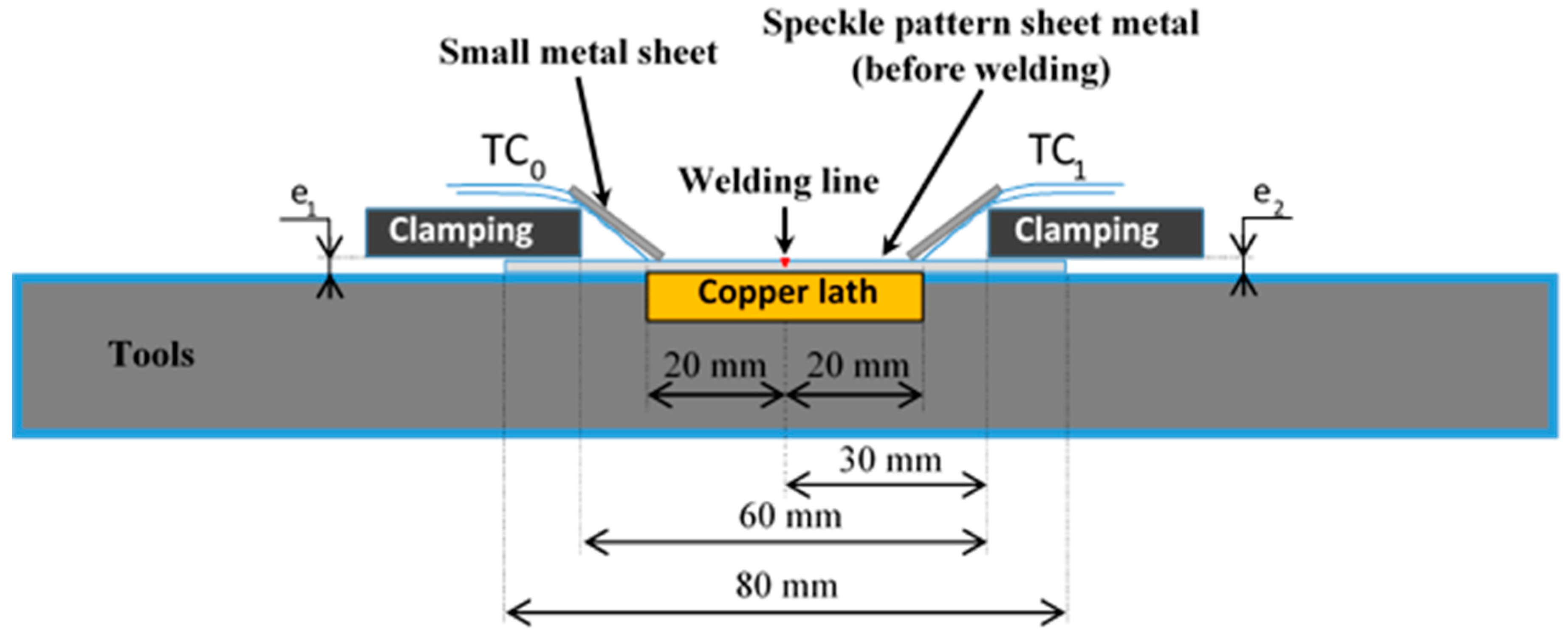
Figure 2.
Electric parameters for one welding sequence (during 0.1 s).
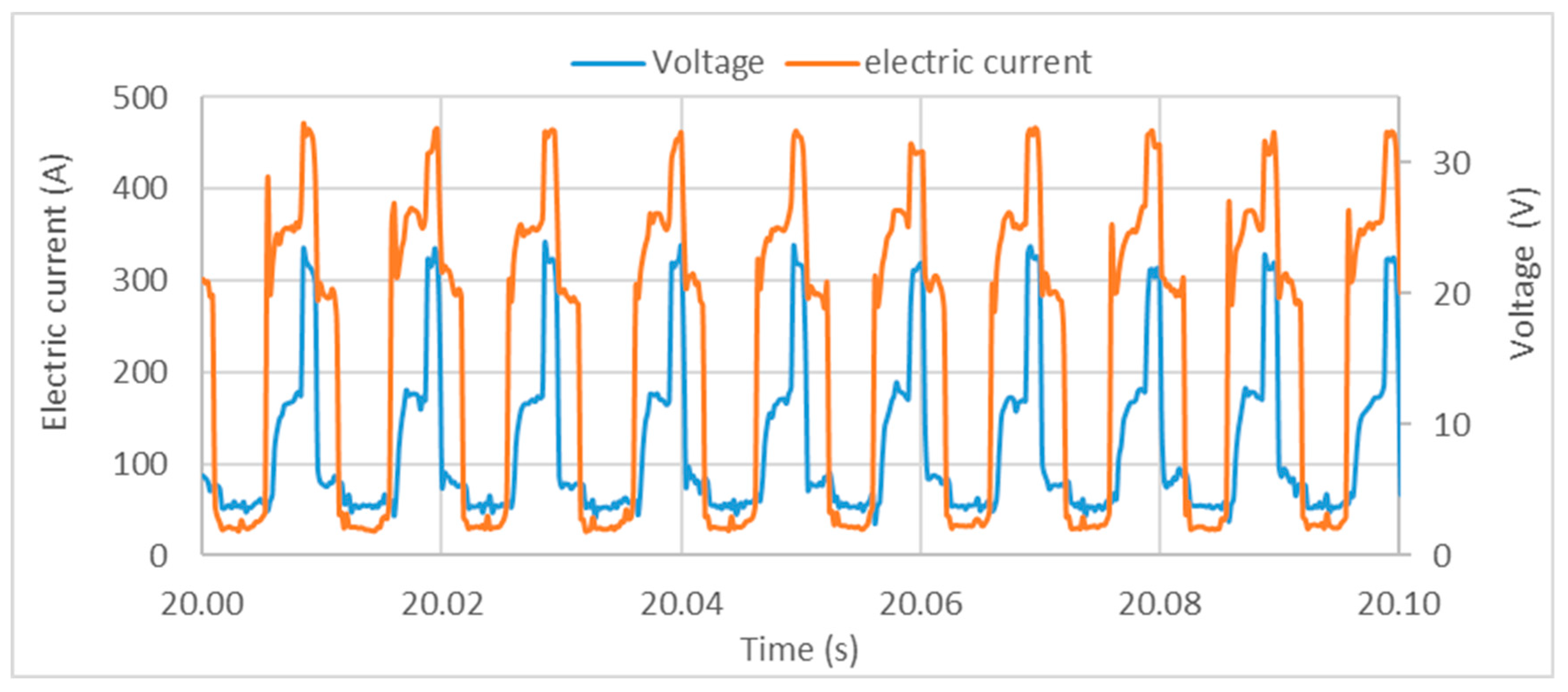
Figure 3.
Macrographic sections of the weld.
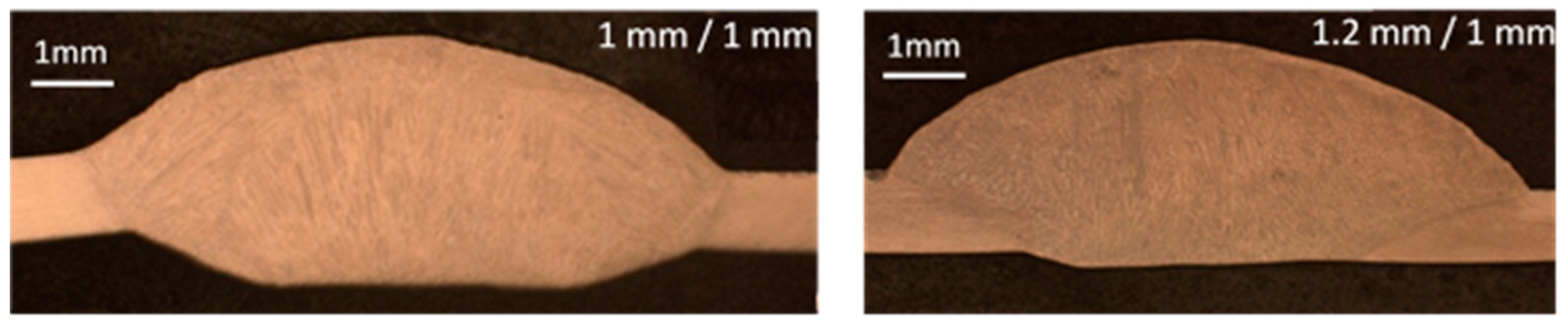
Figure 4.
Schematic of macrographic measurements (weld seam dimensions).
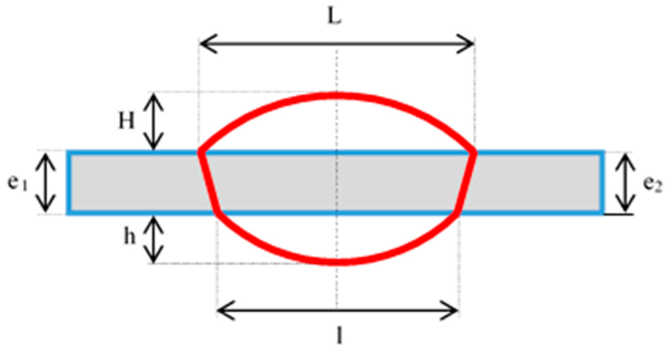
Figure 5.
Local model: mesh and welding region.
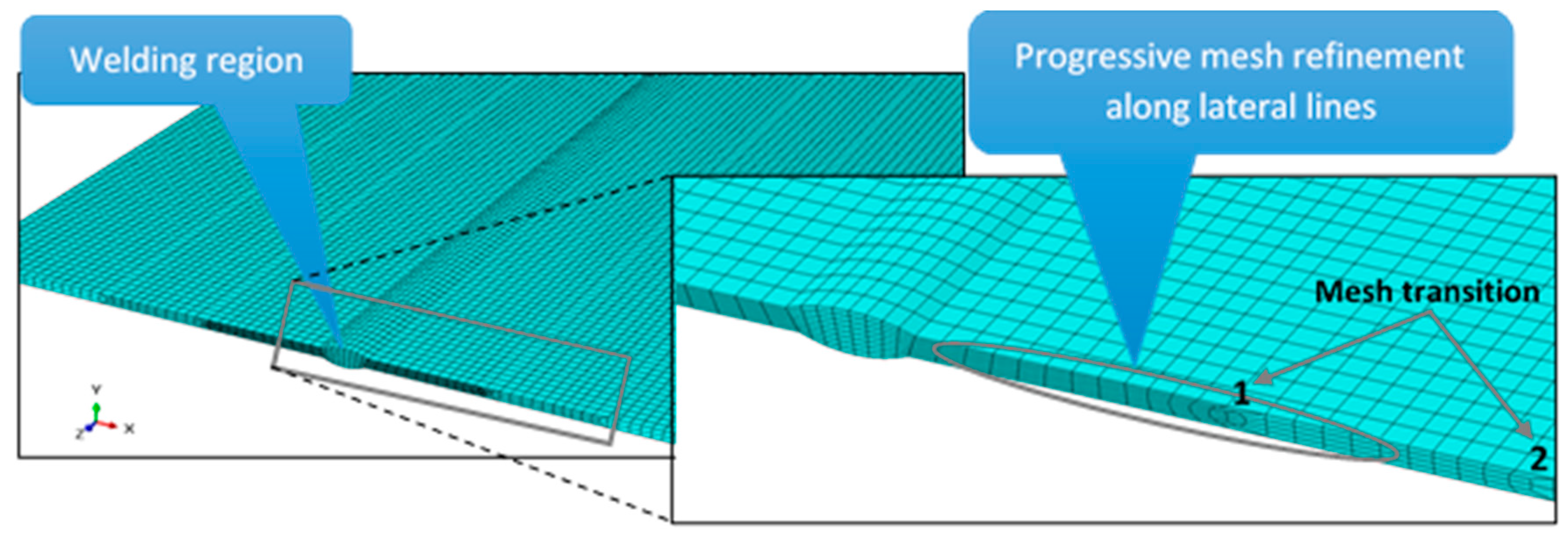
Figure 6.
Mechanical properties of 304L stainless-steel used in the bilinear isotropic strain hardening model [19].
Figure 6.
Mechanical properties of 304L stainless-steel used in the bilinear isotropic strain hardening model [19].
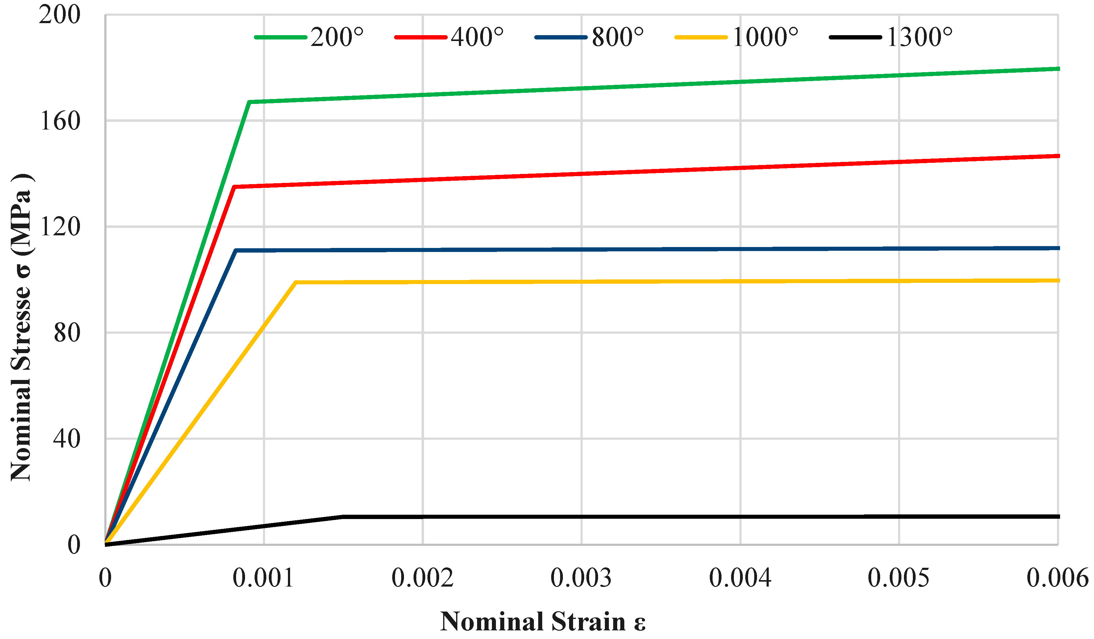
Figure 7.
Prismatic source composed of a trapezoid and two disc segments.
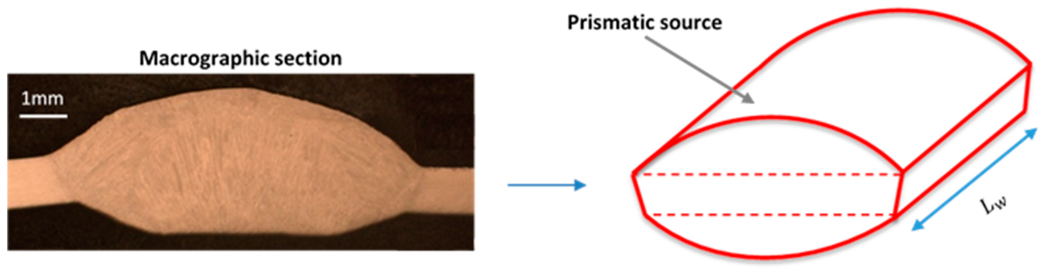
Figure 8.
Comparison between experimental macrostructure and shape of predicted molten zone MZ.
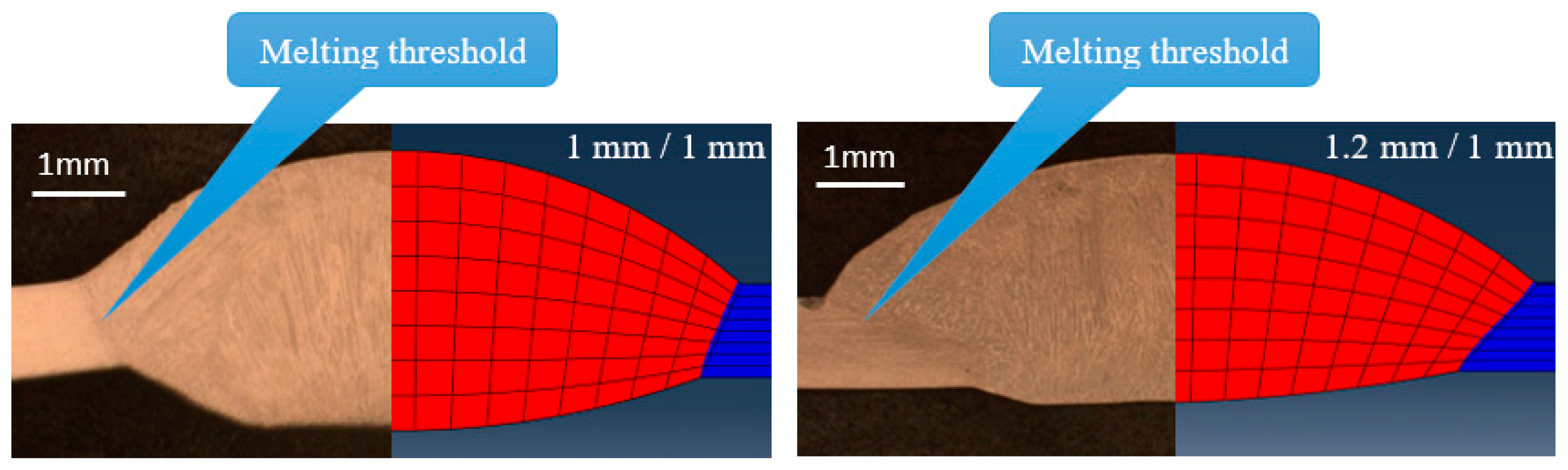
Figure 9.
Thermal parametric study: temperature at 20 mm from seam axis, for various values of h, case 1 mm / 1 mm.
Figure 9.
Thermal parametric study: temperature at 20 mm from seam axis, for various values of h, case 1 mm / 1 mm.
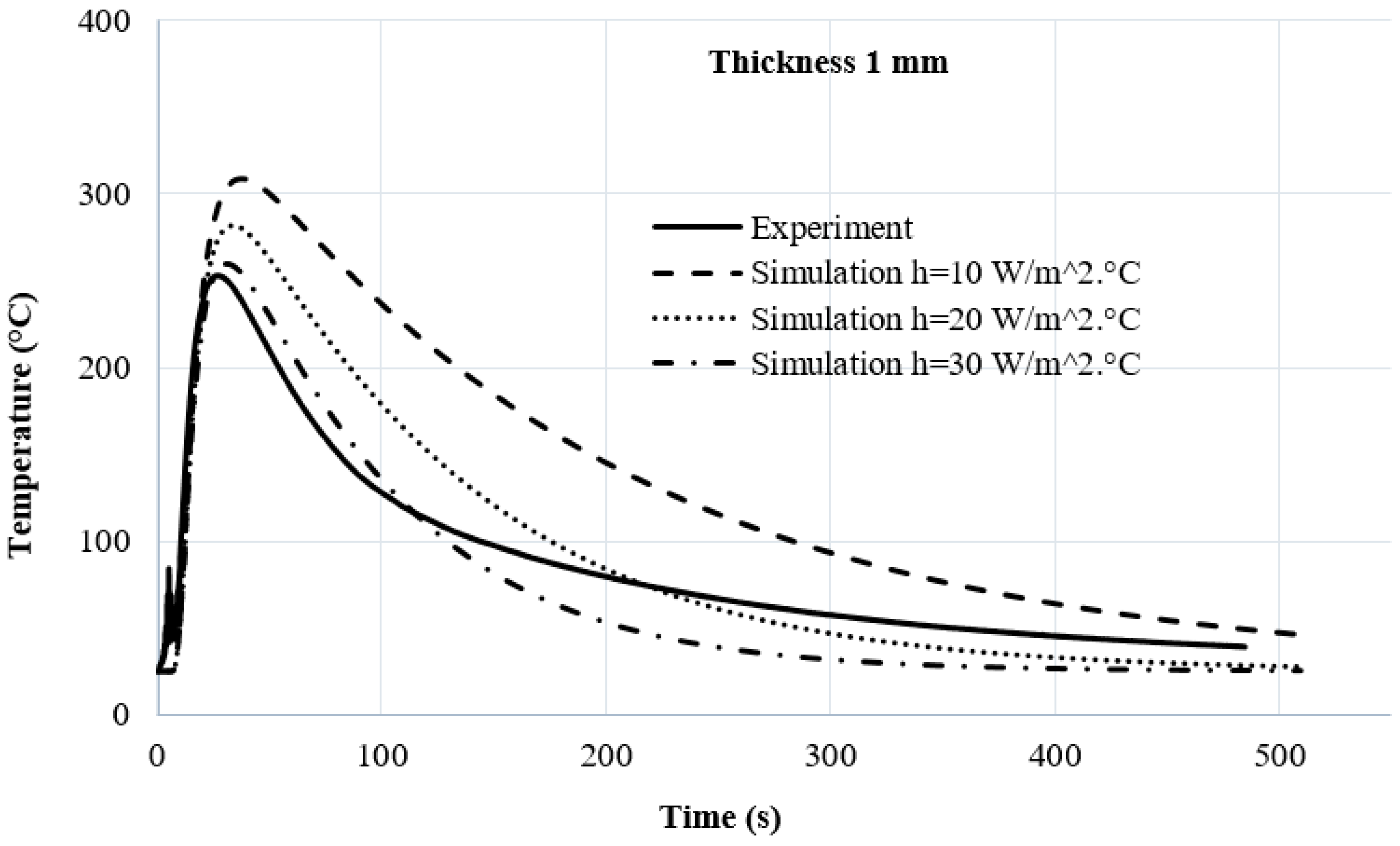
Figure 10.
Thermal parametric study: temperature at 20 mm from the seam axis, for various values of h, case 1.2 mm/1 mm.
Figure 10.
Thermal parametric study: temperature at 20 mm from the seam axis, for various values of h, case 1.2 mm/1 mm.
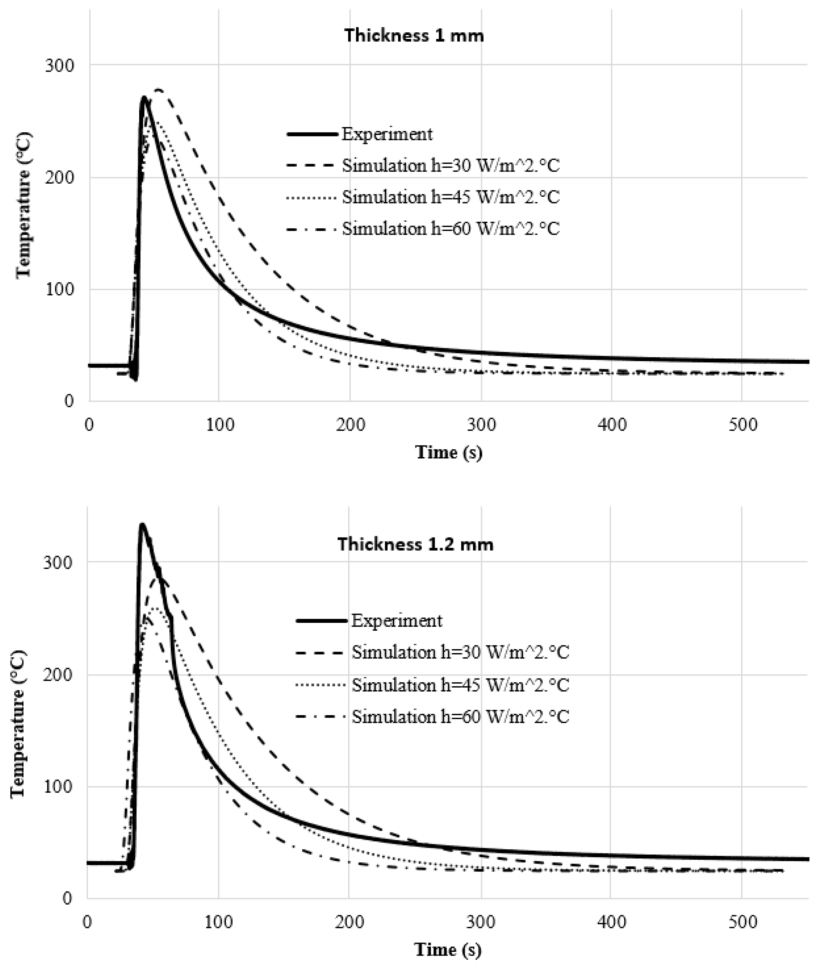
Figure 11.
Numerically calculated displacements and deformation shape.
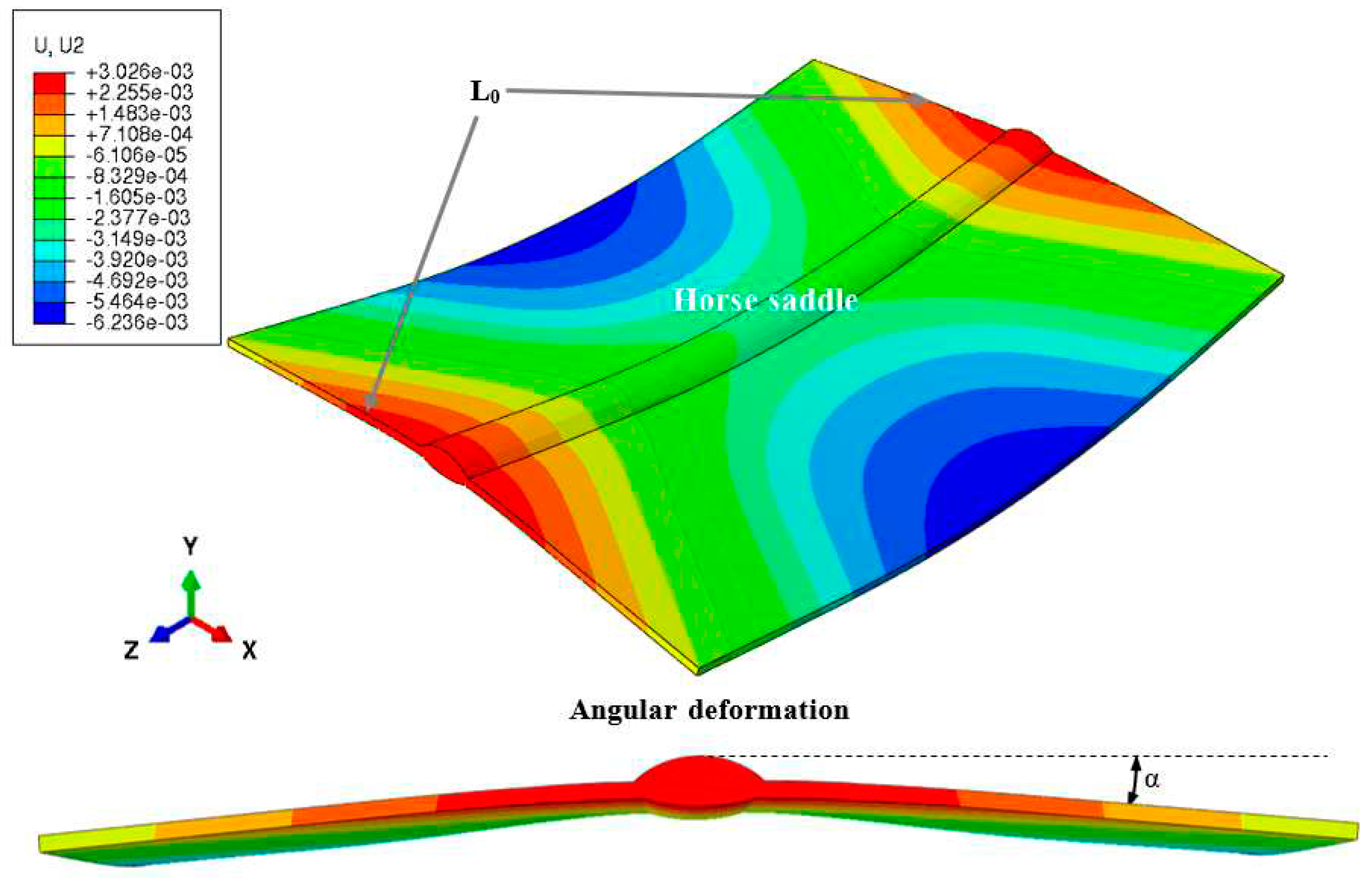
Figure 12.
Comparison between computed results and DIC displacements along line L0, case 1 mm / 1 mm.
Figure 12.
Comparison between computed results and DIC displacements along line L0, case 1 mm / 1 mm.
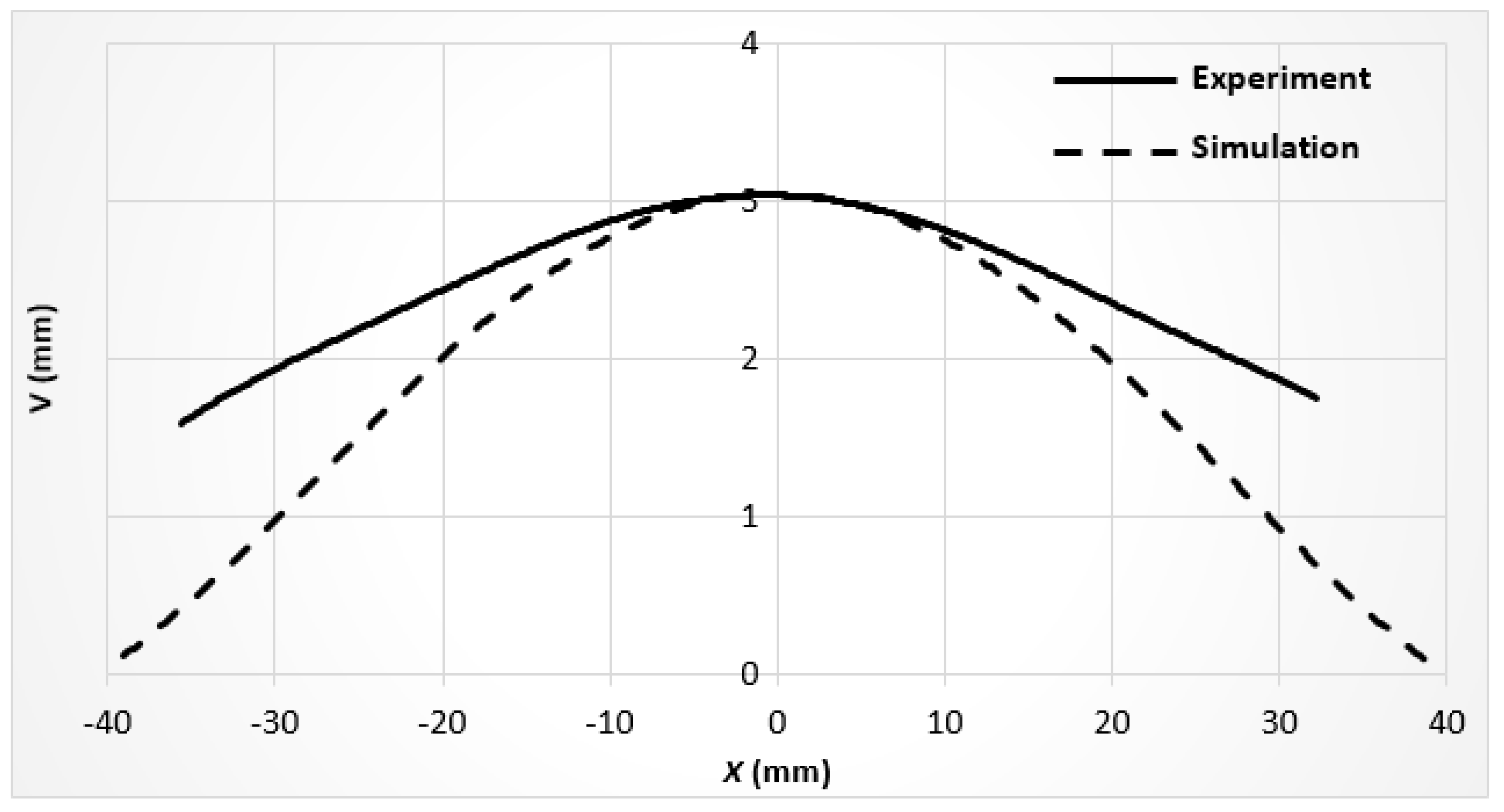
Figure 13.
Comparison between computed results and DIC displacements along line L0, case 1.2 mm / 1 mm.
Figure 13.
Comparison between computed results and DIC displacements along line L0, case 1.2 mm / 1 mm.
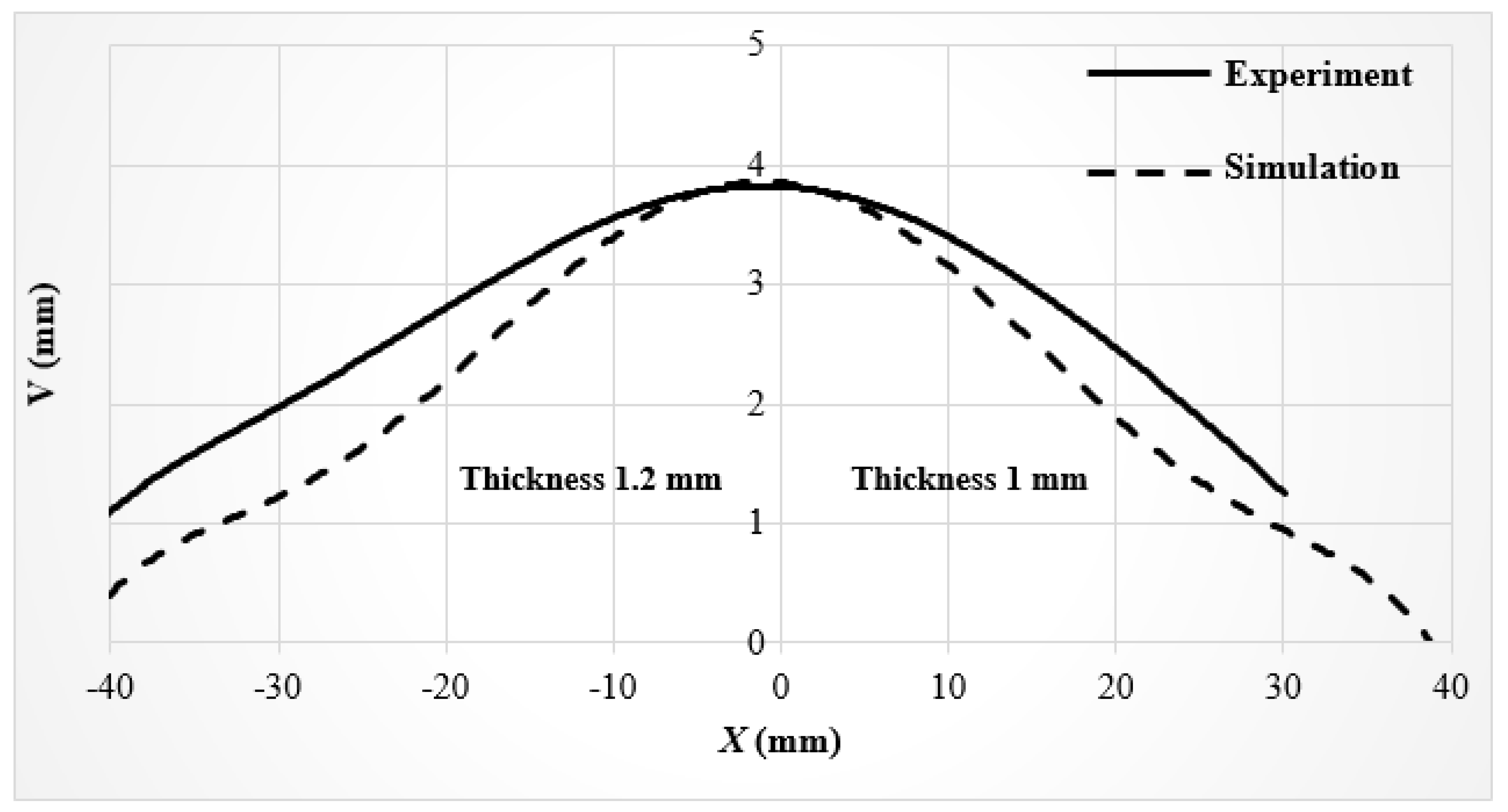

Table 1.
Heat input and welding power.
| Configuration | 1 mm / 1 mm | 1.2 mm / 1 mm |
| Welding energy (kJ/mm) | 0.242 | 0.235 |
| Average power P (kWatt) | 2.62 | 2.55 |
| 0.8 | 0.8 | |
| Heat input (kJ/mm) | 0.194 | 0.188 |
| Average real power (kWatt) | 2.1 | 2.04 |
Table 2.
Numerical values of macrographic measurements to be applied for both welds.
| Configurations | L (mm) | l (mm) | H (mm) | h (mm) | e (mm)=H+h+e1 |
|---|---|---|---|---|---|
| 1 mm / 1 mm | 8.05 | 7.08 | 1.43 | 0.57 | 3 |
| 1.2 mm / 1 mm | 7.51 | 5.83 | 1.52 | 0.36 | 3.1 |
Table 3.
Number of nodes, mesh elements and total CPU time for calculation.
| Configurations | Number of nodes | Nnumber of elements | Total CPU time (secondes) |
|---|---|---|---|
| 1 mm / 1 mm | 56762 | 47100 | 52700 |
| 1.2 mm / 1 mm | 58782 | 48800 | 61600 |
Table 4.
Maximum temperatures measured by thermocouples placed at 20 mm from the weld line.
| Configurations | Thickness (mm) | Maximum measured Temperature (°C) |
|---|---|---|
| 1 mm / 1 mm | 1 | 254 |
| 1 | ||
| 1.2 mm / 1 mm | 1.2 | 335 |
| 1 | 272 |
Table 5.
Relative difference between measured and calculated maximum temperatures for various values of the h, case 1 mm / 1 mm.
Table 5.
Relative difference between measured and calculated maximum temperatures for various values of the h, case 1 mm / 1 mm.
| Convective heat transfer coefficient h (W.m-2.°C-1 ) | Relative difference in the maximum temperatures (%) |
|---|---|
| 10 | 22 |
| 20 | 11.3 |
| 30 | 2.6 |
Table 6.
Relative differences between measured and calculated maximum temperatures for different values of h, case 1.2 mm / 1 mm.
Table 6.
Relative differences between measured and calculated maximum temperatures for different values of h, case 1.2 mm / 1 mm.
| Convective heat transfer coefficient h (Watt.m-2.°C-1) | Relative difference between the maximum temperatures (%) | |
|---|---|---|
| Thickness 1.2 mm | Thickness 1 mm | |
| 30 | 13.7 | 3.1 |
| 45 | 22.3 | 8 |
| 60 | 25.1 | 12.7 |
Table 7.
Comparison of calculated (FEM) and measured (DIC) deformation angles along line L0.
| Configurations | Experiment | Simulation | ||
|---|---|---|---|---|
| 1 mm / 1 mm | 1 mm | 1 mm | 1 mm | 1 mm |
| 2.7° | 2.8° | 3° | 3° | |
| 1.2 mm / 1 mm | 1.2 mm | 1 mm | 1.2 mm | 1 mm |
| 4.9° | 6.1° | 5° | 5.8° | |
Disclaimer/Publisher’s Note: The statements, opinions and data contained in all publications are solely those of the individual author(s) and contributor(s) and not of MDPI and/or the editor(s). MDPI and/or the editor(s) disclaim responsibility for any injury to people or property resulting from any ideas, methods, instructions or products referred to in the content. |
© 2023 by the authors. Licensee MDPI, Basel, Switzerland. This article is an open access article distributed under the terms and conditions of the Creative Commons Attribution (CC BY) license (http://creativecommons.org/licenses/by/4.0/).
Copyright: This open access article is published under a Creative Commons CC BY 4.0 license, which permit the free download, distribution, and reuse, provided that the author and preprint are cited in any reuse.


