Approach of Trajectory Generation Based on Waypoint Information for a Highly Automated Vehicle

The development and use of highly automated vehicles (HAV) in agriculture is a highly important task because of the lack of machine drivers and unsatisfactory level of their qualifications, reducing the impact of harmful factors on employees of agricultural enterprises. HAVs allow to avoid these problems: increase productivity and the efficiency of seasonal use of equipment, and reduce the impact of harmful factors on people. Modern HAVs in agriculture are based on the following methods: parallel driving according to geo coordinates without automatic turning and without obstacles tracking, and on technical vision without the use of a geographic information system (for example Cognitive AgroPilot) and a digital field map, which makes it impossible to generate the optimal path around the field.

Keywords:

Subject: Computer Science and Mathematics - Artificial Intelligence and Machine Learning

1. Introduction

The agricultural market is one of the most profitable and important, along with the fuel and energy resources extraction [1]. The need to reduce the cost of production increases as the increase of production scale. Also, is the need to reduce the number of people engaged in hard or unhealthy work. One of the most promising opportunities for increasing productivity is the development of highly automated vehicles (HAV) [2]. Processing agricultural fields with HAV has the following key advantages:

Increasing the efficiency of processing because HAVs do not require breaks and rest and do not need to stop working in the dark;
Reducing the cost of maintaining a large staff of drivers [3];
Reducing the cost of growing agriculture crops also allows to lower the price of the final product, which means get a more competitive position in the market [4];
Reducing harmful factors for drivers when processing a field with chemicals [4].

At the moment, the market for unmanned vehicles is rapidly growing in several industries:

passenger taxis and other types of passengers transporting,
transportation of cargos inside closed areas,
transportation of cargos between cities,
mining dump trucks,
vehicles for transporting cargos in areas with hard climates,
self-propelled vehicles,
agriculture, etc.

There are two approaches to creating an HAVs. The first of them is the development of a completely proprietary automotive platform, initially designed for autonomous driving [5]. This approach has the advantage that the vehicle systems are initially designed to be controlled without the participation of the driver, and there is no need to repeat the driver’s actions (pressing the pedals, turning the steering wheel, shifting the gearbox selector, etc.). But this approach has a significant problem: in most times, it is difficult and expensive to organize large-scale assembly of vehicles. The second approach is the conversion of an existing vehicle in the presence of universal methods and tools for modification [6,7].

Authors describe in this article developed models and tools for software control of vehicle systems based on the modification of the UAZ Patriot vehicle [8].

The main aim of this project is to increase the speed of development of the subsystem for path following for HAV through the automated selection of the main parameters of the algorithm for generating highly discretized oriented coordinates of the movement trajectory based on waypoints generated automatically or manually in the map editor.

Often, a HAV is forced to vary from a pre-calculated route because of the detection of static or dynamic obstacles or the vehicle operator taking over control [9]. The HAV must continue moving and return to its original trajectory after avoiding obstacles or returning control. Calculating a new trajectory is a difficult task.

To solve this problem, the authors developed the complex algorithm that combines methods of generating waypoint information and trajectory generation, considering vehicle kinematics and the possibility of optimally continuing the route after varying from it.

Using a real vehicle to test the developed algorithms generating waypoint information and trajectory generation is extremely inefficient and time-consuming. It is much more convenient to use various computer-aided design systems. The authors developed the vehicle simulator that allows to simulate the trajectory of the vehicle movement by setting the target steering angle and the vehicle speed.

The authors tested the operation of the algorithm in the developed simulator. The proposed simulator allows to visualize the trajectory of a vehicle based on waypoint information through integration with the HAV control system at the level of application software interfaces.

The article is organized as follows: Section 2 presents an analysis of the related works, Section 3 describes the proposed approach, Section 4 contains a detailed description of the HAV architecture and the circuitry used solutions, Section 5 presents the results of experiments with the Q-learning algorithm.

2. Related works

A HAV control system can be represented as an end-to-end solution [10] implemented based on machine learning tools, such as reinforcement learning. However, neural networks have low explanatory power in decision-making mechanisms, which is important when solving HAV control tasks. It is important to discover the causes when engineers analyzing road accidents. Engineers must understand the criteria for deciding in that situation. End-to-end solutions also cannot be widely used because of the low performance of the computing modules used on a vehicle board [11].

The classical approach to the design of HAV involves the creation of models, methods, and programs based on the management of data flows during the control cycle. So, it is necessary to develop and use models for processing data generated by sensors at each stage of processing [11].

One of the most important stages in the design of a HAV control system is the path following subsystem. The path following subsystem accepts a list of low-sample path coordinates (oriented waypoints), and information about the vehicle itself (dimensions, turning radius).

2.1. Algorithms for generating HAV movement waypoints

Waypoints can be got in several ways. First, they are specified manually in specialized trajectory map editors for HAV [11,12]. Second, they can be generated automatically by path planning algorithms based on the task features and information about the environment, for example, using Q-learning algorithms [13], RRT algorithms [14], or their modifications [15,16,17,18].

The relevance of this work is determined by the need to build an intelligent system for HAV control. Autonomous decision-making task to construct the optimal trajectory of movement with context of the environment arise in the absence of constant contact between the operator and the HAV.

The theoretical basis for creating intelligent HAV control systems can be reinforcement learning (RL). A detailed classification of RL algorithms is given in [19,20,21]. Reinforcement algorithms are used only for waypoint generation and not for HAV control itself. Some researchers [19] have emphasized the effectiveness of RL methods for a certain class of problems. For example, when there are a few permissible environmental states. The SARSA method and the Q-learning method are often noticed among such methods. They differ from each other in that the SARSA method uses control with a single strategy, and the Q-learning method uses control with a separate strategy, which increases the stability of the algorithm.

The works [20,22] note that the SARSA and Q-learning methods show similar results. Therefore, the Q-learning method [23,24] is used in this paper to study the possibility of applying RL methods to solve the of problem of generating a HAV trajectory based on the waypoint.

2.2. Algorithms for constructing a trajectory based on waypoints information

Various algorithms can generate the optimal HAV trajectory based on waypoints information. Such algorithms are mainly based on:

Bezier curves [25],
Dubins Curves [26],
Reeds-Shepp curves [27].

Bezier curves were proposed in 1962 and are mathematical curves defined by control points. Bezier curves are the easiest to implement. The N control points are related to the P order of the curve by the dependence

N = P + 1

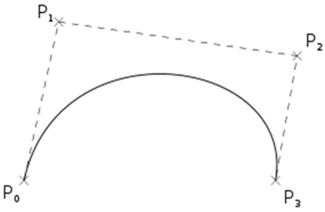
A cubic Bezier curve is suffices to connect two points that are the origins of vectors on a plane. If a cubic curve is defined by four points

P 0 - P 3

(Figure 1), then the curve can connect two control points P0 and

P 3

, feeling them toward intermediate control points

P 1

and

P 2

, respectively [25].

The advantage of moving along Bezier curves is only the relative smoothness of the trajectory. The disadvantages are much greater:

Ineffective with strong changes of direction.
The need to create algorithms capable of selecting intermediate control points optimally.
Difficulty in considering the minimum turning radius of a vehicle.
Possibility of movement in only one direction.

Dubins curves are more suitable for solving the problem. Dubins curves were proposed in 1957 [26]. Like Bezier curves, they can connect two points on a plane, each of which is given a travel direction. An important input parameter of this algorithm is the maximum curvature of the trajectory. Curvature of the trajectory is limited by the minimum turning radius of the vehicle.

Dubins curves comprise only two components: straight lines and sections of maximum curvature, which are arcs of circles. The example of Dubins curves is shown in Figure 2.

The most important advantage of generating a trajectory based on Dubins curves is the ease of considering the physical limitations of the vehicle on the minimum turning radius. In addition, Dubins curves make it possible to generate trajectories with the optimal length.

The disadvantage is the impossibility of planning a path with a change of direction during movement. Dubins curves make it difficult to use the reverse vehicle function.

Reeds-Shepp curves are also effective to achieve the shortest length of the resulting path. Reeds-Shepp curves are introduced in 1990. These curves are like Dubins curves but allow to generate of a trajectory considering the functions of a vehicle to move forward and backward.

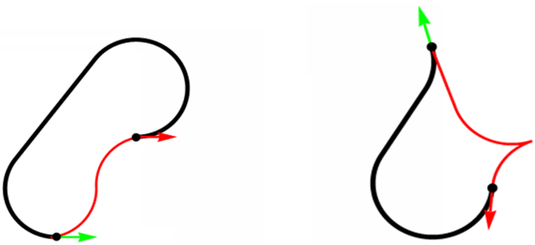
The ability of the Reeds-Shepp curves to use the both directions of movement in various cases can provide a significant reduction in the length of the resulting path. This advantage is clearly visible in Figure 3, where the red line shows the path based on the Reeds-Shepp curves, and the black line shows the path based on the Dubins curves.

Reeds-Shepp curves also have disadvantages. The main one is the probability of generating a trajectory containing an excessive number of points at which a change in the direction of movement of the HAV should occur. This leads to an increase in movement time in various cases compared to Dubins curves. This occurs because the vehicle cannot immediately stop or start moving. The presence of a gearbox on a vehicle also has a negative impact on the speed of changing direction.

A less significant disadvantage is the relative complexity of the software implementation of Reeds-Shepp curve generators.

3. Proposed approach

3.1. Q-learning algorithm for generating HAV trajectory waypoints information

Agent is a HAV model, which learns and decides about choosing the direction of movement in a discrete 2D space. Environment is an agricultural field through which the agent needs to move. Reward is a numerical value that is returned by the environment depending on a successful or not successful agent action [28].

Agent and environment interact in time and form a sequence of steps

t = 1, 2, . . ., n

. Agent receives information at each t step about the state

s_{t} \in S

(observation result) of the environment as a reaction to the performed action

a_{t} \in A

. At the next step

t + 1

, the agent receives a reward

r_{(} t + 1) \in R

and moves to the next state

s_{(} t + 1) \in S

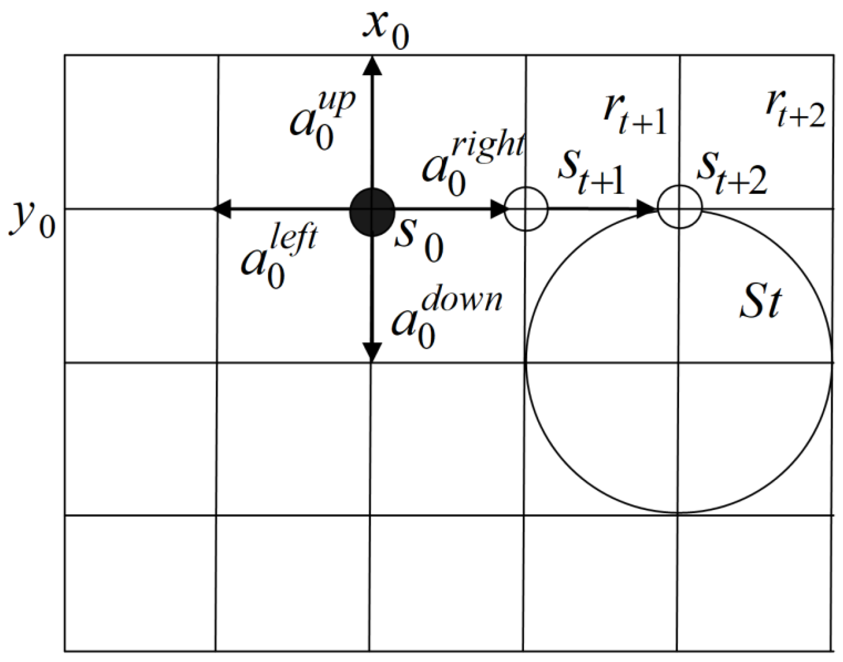
Figure 4 shows a simplified model of the environment for generating the HAV trajectory. The initial state

s_{0}

and actions of the agent

a_{t} = {a_{t}^{u p}, a_{t}^{d o w n}, a_{t}^{l e f t}, a_{t}^{r i g h t}}

available in any state of the environment are shown. If the agent is in a certain state (Figure 2) and chooses an action

a_{0}^{r i g h t}

, then the environment goes into the state

s_{(} t + 1)

and the agent receives a reward

r_{(} t + 1)

The formulation of the problem considers that the number of states of the environment is limited and is calculated based on data on the dimensions of the width and length of the geometry of an agricultural field which along the agent moves and the size of the grid. Parametrically, the state is determined by the agent coordinates at a certain step in the formation of a learning episode

s_{t} = < x_{t}, y_{t} >

(HAV movement trajectory).

The set of types of rewards R is determined as the following possible situations:

The current action takes the agent outside the boundaries $(r_{t}^{o u t} \in R)$ of the simulation environment. This reward has a negative value, because is a penalty.
Changing the HAV coordinates $(r_{t}^{s h i f t} \in R)$ .
The agent enters an area marked as an obstacle $(r_{t}^{b a r r i e r} \in R)$ . This reward is also a penalty.
The HAV arrives at the target route completion point $(r_{t}^{t} a r g e t \in R)$ .

The main aim of the proposed algorithm based on reinforcement learning is to generate the optimal trajectory of the HAV. The HAV must avoid falling into zones marked as obstacles and reach the end point of the route.

The algorithm for generating the HAV trajectory is associated with the concept of an episode. An episode is understood as a sequence of repeated interactions of the HAV with the environment. The episode is a finite Markov process:

(s_{0}, a_{0}, 0) \to (s_{1}, a_{1}, r_{1}) \to (s_{2}, a_{2}, r_{2}) \to . . . \to (s_{T}, a_{T}, r_{T}),

where T is the moment of the episode completion.

The generated episode ends in the following cases:

The trajectory of the simulated HAV crosses the area marked as an obstacle.
The HAV reached the final point of the route and the algorithm generates the optimal trajectory.
The episode length has reached its maximum..

The total income from time t to the end of the episode is calculated using the following equation:

G_{t} = r_{t + 1} + γ \cdot r_{t + 2} + γ^{2} \cdot r_{t + 3} + . . . + γ^{T - t - 1} \cdot r_{T} = \sum_{k = t + 1}^{T} γ^{k - t - 1} \cdot r_{k},

where

γ = \bar{(0, 1)}

is the discount factor for the received reward.

The Q-learning algorithm is based on the Q-table, which contains the optimal values of the action quality function

q_{*} (s, a)

, calculated using the Bellman optimality equation:

q_{*} (s, a) = \sum_{\overset{´}{s}, \overset{´}{r}} p (\overset{´}{s}, \overset{´}{r} | s, a) (\overset{´}{r} + γ \cdot m a x_{\overset{´}{a}} q_{*} (\overset{´}{s}, \overset{´}{a})),

where

\overset{´}{s}, \overset{´}{r}

is a next state and a reward received by the HAV, respectively. Expression

p (\overset{´}{s}, \overset{´}{r} | s, a)

specifies the dynamics of the environment and determines the probability of transition to state

\overset{´}{s}

and receive of reward

\overset{´}{r}

, then the HAV is in state s and chooses action a.

Table 1 shows the Q-table example.

Table 1 shows four HAV actions:

upward movement,
downward movement,
movement to the right,
movement to the left.

The number of states is determined by the number of nodes in the discrete grid environment in which the HAV exists.

Since the model of the environment is unknown according to the conditions of the current task, the information about the environment of the HAV must be reached through repeated attempts to construct trajectories (generate episodes).

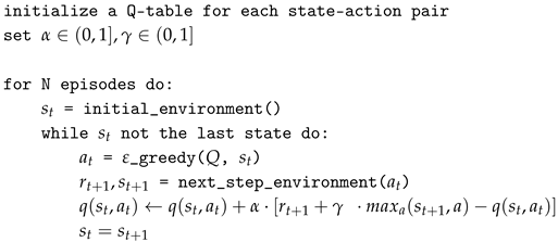
The pseudo-code of the Q-learning algorithm for generating the HAV trajectory has the following form:

The algorithm begins from initializing the Q-table with zero values. Next, values of the learning rate coefficients

α

and reward discounting coefficients

γ

received by the agent at each learning step are assigned. The for loop generates a set of episodes. The initial state is initialized for each episode. HAV always starts moving from the specified position.

The while loop of the algorithm sequentially forms a separate episode. The next action is determined using an epsilon-greedy algorithm. With some probability

ε

the action of the HAV is chosen randomly, otherwise as an argument of the function

{m a x}_{a} (s_{t}, a)

After determining the action, the simulation system performs the next step, and the environment returns the next state

s_{t + 1}

and reward

r_{t + 1}

. The behavior of the environment is deterministic in this task. The Q-table values are updated according to the function given in the algorithm pseudocode.

Q-table contains the optimal values of the action cost function after the execution of the various algorithms episodes N. So, it is possible to construct the trajectory of the HAV movement using a “greedy” strategy. Table 2 contains an example of a completed Q-table.

As you can see from Table 2:

Step 1.: Let the initial state correspond to coordinates (20,20). The grid size is 10 units. The maximum of the action quality function occurs to the ”downward movement” action for the initial state. This action leads to the state (20,30). Y coordinate increases by one step, because the origin (0,0) is in the upper left corner of the coordinate plane.
Step 2.: The maximum of the quality function corresponds to the ”movement to the right” action for the (20,30) state. There is a transition to the next state (30,30).
Step 3.: The ”downward movement” action has the maximum value for the (30,30) state. The next state is (30,40).
Step 4.: Next, the ”movement to the left” action has the maximum value for the state (30,40). The algorithm stops because the state (20,40) is a last point of the trajectory.

Thus, the waypoint information of the HAV movement across the field is formed after executing the proposed algorithm as a vector of points, each of which corresponds to a geographic coordinate.

3.2. Algorithm for trajectory generation based on waypoint information and Reeds-Shepp curves

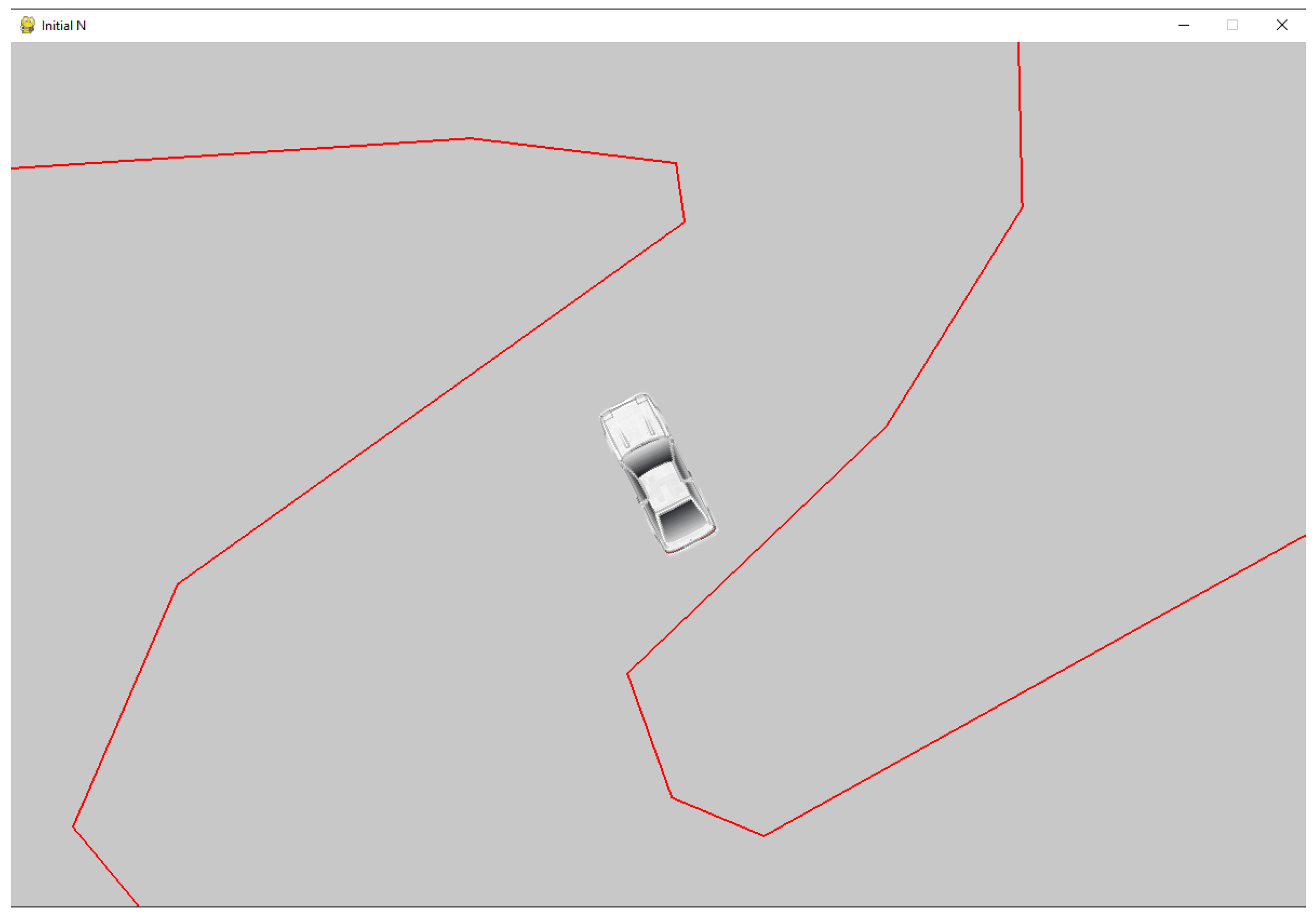
The authors develop the simulator that considering the basic parameters of the route (obstacles), road width, and vehicle parameters (dimensions and turning radius) to determine the parameters of the implemented algorithm based on Reeds-Shepp curves (rounding and sampling step).

A receiving vector of highly discretized points describing the planned trajectory can be given to the input of a route following algorithm, which is based on a method for minimizing the deviation between the actual and calculated trajectories.

Since the HAV is assumed to move on the ground, it is suffices to use only two axes for modeling. The resulting HAV model in a simplified form is described by the following five parameters: position in the plane, speed on both axes, and rotation angle. Each parameter is recalculated on each frame, and has a dependence on the previous one.

The rotation angle is calculated using the following equation:

α = α^{'} + \frac{β}{10}

where

α^{'}

is the previous angle value;

β

is the vehicle turning ratio.

The velocities relative to the axes are calculated based on the resulting angle:

x_{1}^{'} = (x_{0}^{'} - \frac{c o s (α) - v}{2}) \cdot 0, 7 \cdot \frac{c o s (α) \cdot v}{2}

y_{1}^{'} = (y_{0}^{'} - \frac{s i n (α) - v}{2}) \cdot 0, 7 \cdot \frac{s i n (α) \cdot v}{2}

where

x_{0}^{'}

and

y_{0}^{'}

are the speed in the previous calculation for x and y, respectively.

The coordinates are received by adding the previous coordinates with the speed:

x_{1} = x_{0} + x_{1}^{'}

y_{1} = y_{0} + y_{1}^{'}

Figure 5 shows an example of how the proposed simulator works:

Waypoints information is converted into a specific route at intermediate stages of data processing, considering the following HAV characteristics: turning radius, dimensions, and the ability to use reverse gear (reversing). This route comprises highly discretized waypoints determined by the algorithm parameters and vehicle maneuverability. The algorithm for constructing Dubins curves [26] is used for the route on which the use of reverse gear is not expected, and the Reeds-Shepp curves [27,29] are used for the route the movement of which requires reversing. The algorithm for constructing Reeds-Shepp curves is the main one in this work.

The proposed algorithm takes the waypoint information as input and builds vectors on the plane from the HAV to the first two unreached points in the sequence and determines the angle between the course of the vehicle and the sum of vectors on the plane to the points depending on the proportionality coefficient.

The vector on the plane is calculated using the following equation:

\bar{v} = \frac{{\bar{v}}_{1} \cdot α + {\bar{v}}_{2} \cdot (1 - α)}{2}

where

{\bar{v}}_{1}

and

{\bar{v}}_{2}

are vectors from the HAV to the first point and from the first point to the second, respectively;

α

is the proportionality coefficient.

After this, the angle between the heading and the resulting vector is calculated and multiplied by the steering coefficient to correspond to the maximum angle of rotation of the HAV wheels.

Checking to reach the nearest points is performed by calculating the vehicle distance for this point. If the point has approached the specified threshold value, then the point is marked as passed.

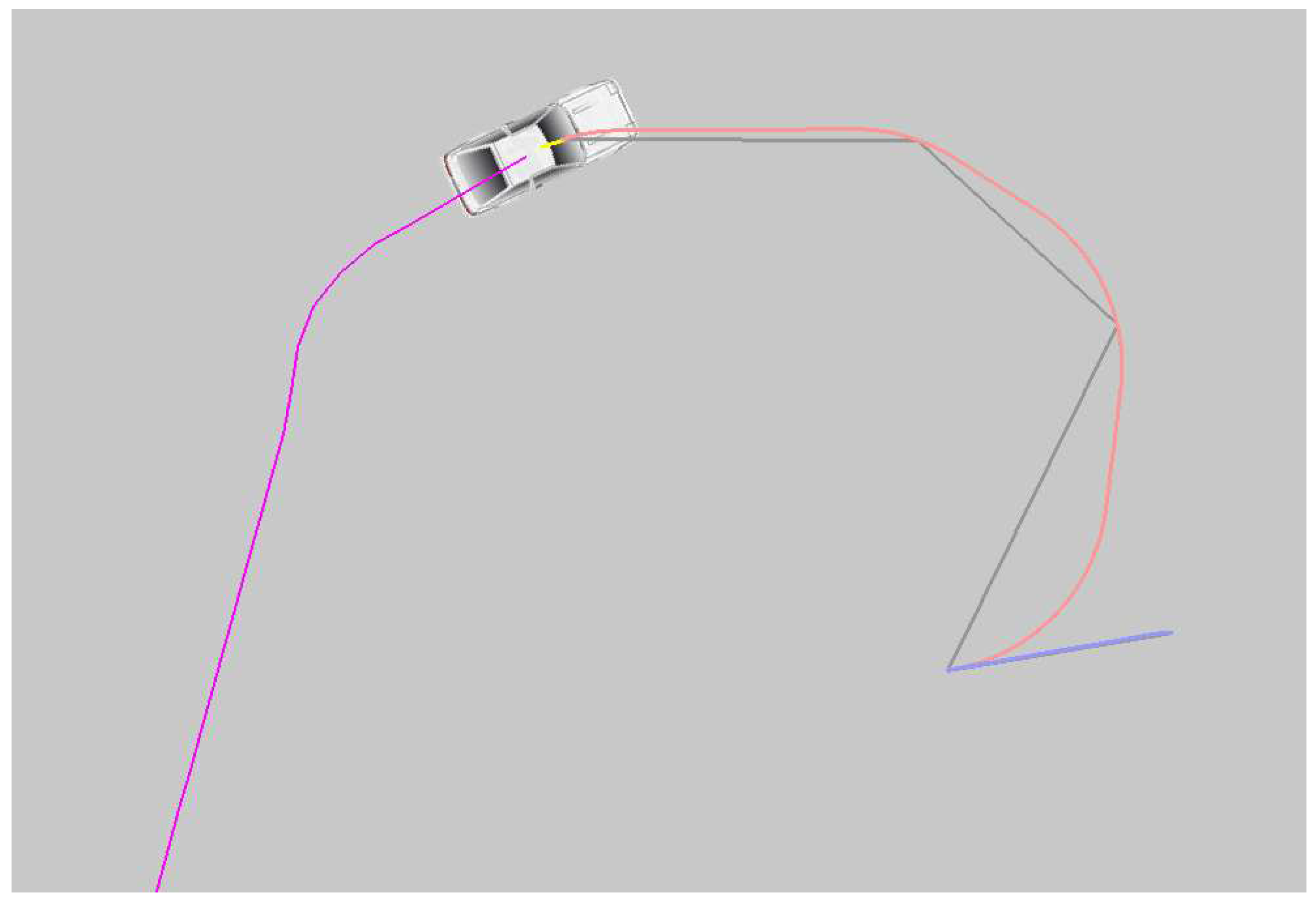
Figure 6 shows an example of how the proposed algorithm works in a simulation environment.

Purple illustrates the traveled path, red and blue illustrate the high-sample path planned using the Reeds-Shepp algorithm, and gray illustrates the low-sample path set by the proposed Q-learning algorithm.

4. System architecture and circuit solutions

SAE International classification of levels of autonomy for automotive engineers identifies five levels of autonomy [30]. This paper describes models and methods for converting a zero-level vehicle (without automation) into a third (conditional automation) or higher (high/full automation), while high reliability and safety requirements are imposed on the system [31]. But not only controllers are implemented for transmitting control actions to the vehicle but also a subsystem for centralized control of the controllers, ensuring their coordinated operation, and tool for emergency stopping the vehicle with an emergency [32]. The microcomputer centrally generates individual commands for the controllers in automatic control mode, providing control over the execution of these commands for safety [33].

Microcomputer in the developed system control signals are transmitted not to individual components, but to a specially designed hardware controller of the HAV to avoid the issues of a microcomputer freezing. This controller checks the correctness of control commands and tracks errors in the system operation, and also implements the transition to manual or remote control mode and performs various safety algorithms, including emergency stops. Thus, all important functions of the autonomous control system are implemented at a low level and remain operational, even without the participation of a computer.

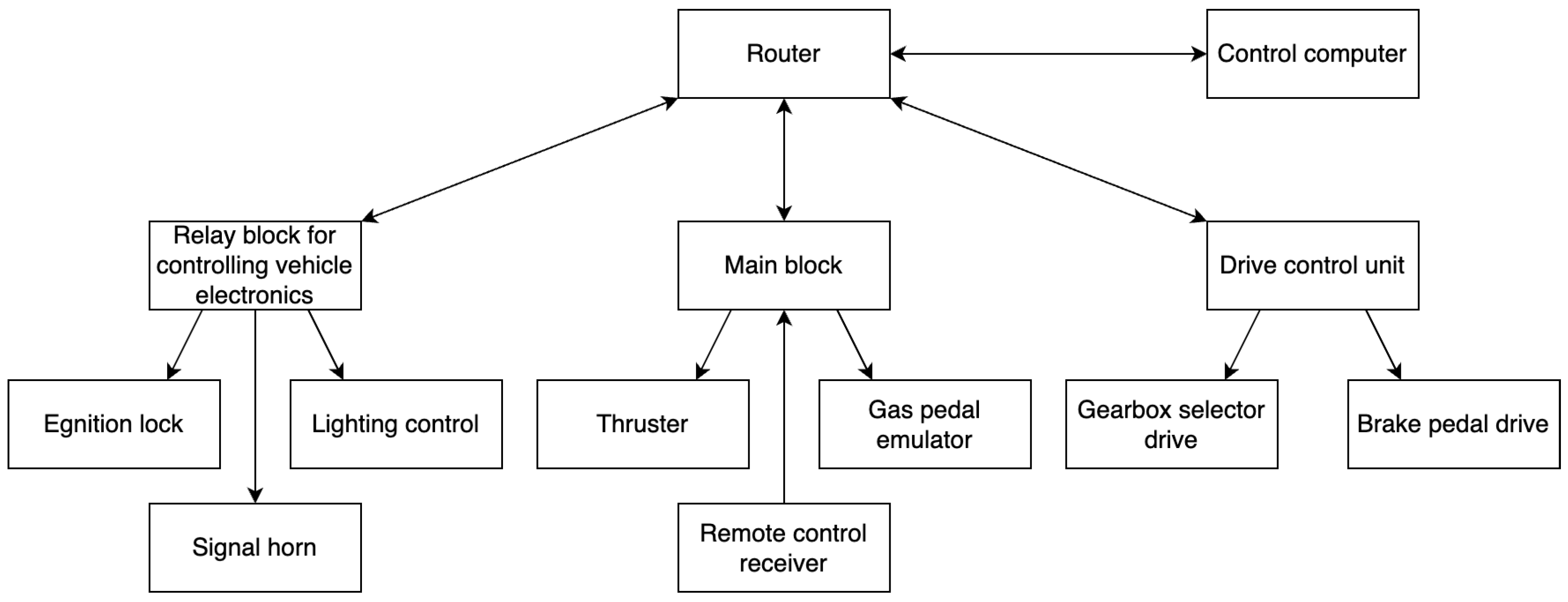
Figure 7 shows the architecture of the command execution subsystem for the HAV.

In the developed command execution subsystem, there are three most important blocks:

The main unit includes a radio receiver for communication with the control panel, connectors for communication with the thruster, and an emulator of the electronic gas pedal. The main unit receives control commands from the HAV control system and ensures coordination of the actions of other units besides controlling these modules.
The drive control unit contains drivers for regulating electric motors, which move the brake pedal and shifting the gearbox selector.
The relay box equipped with eight relay modules, ethernet and CAN interface, and GPIO controls automotive electronics, including the ignition switch, headlights, turn signals and horns.

Each unit is equipped with an ESP32 controller loaded with a specialized program. The connection between these blocks is established through a router using an Ethernet interface. A similar approach is used in popular self-driving electric vehicles from Tesla [34,35].

The drive control unit deserves special attention among all the components. Synchronous motors were chosen for the drives because they are best suited for implementing vector control.

Field-oriented control (FOC) is a method of controlling synchronous and asynchronous motors, not only generating harmonic phase currents (voltages) (scalar control), but also providing control of the rotor magnetic flux [36]. The currents, voltages, and magnetic fluxes of a vehicle are expressed as space vectors within a rotating reference frame (RRF). The operating principle of FOC is based on the machine equations in this RRF. Let us consider the stator equations of an isotropic PMSM in RRF:

\begin{matrix} U_{d s} = R_{s} I_{d s} + (d Ψ_{d s}) / d t - ω_{s} Ψ_{q s}; \\ U_{q s} = R_{s} I_{q s} + (d Ψ_{q s}) / d t - ω_{s} Ψ_{d s}; \\ Ψ_{d s} = L_{d} I_{d s} + Ψ_{P M}; \\ Ψ_{q s} = L_{q} I_{q s}; \end{matrix}

The equation for torque is:

T_{e m} = \frac{3}{2} p (Ψ_{d s} I_{q s} - Ψ_{q s} I_{d s});

Stator current control can comprise two digital PI controllers, followed by some basic math to calculate PWM duty cycles. A decoupling circuit is needed to achieve independent control of each current component since the d and q axes are coupled. PI controllers can be tuned using the optimal value criterion:

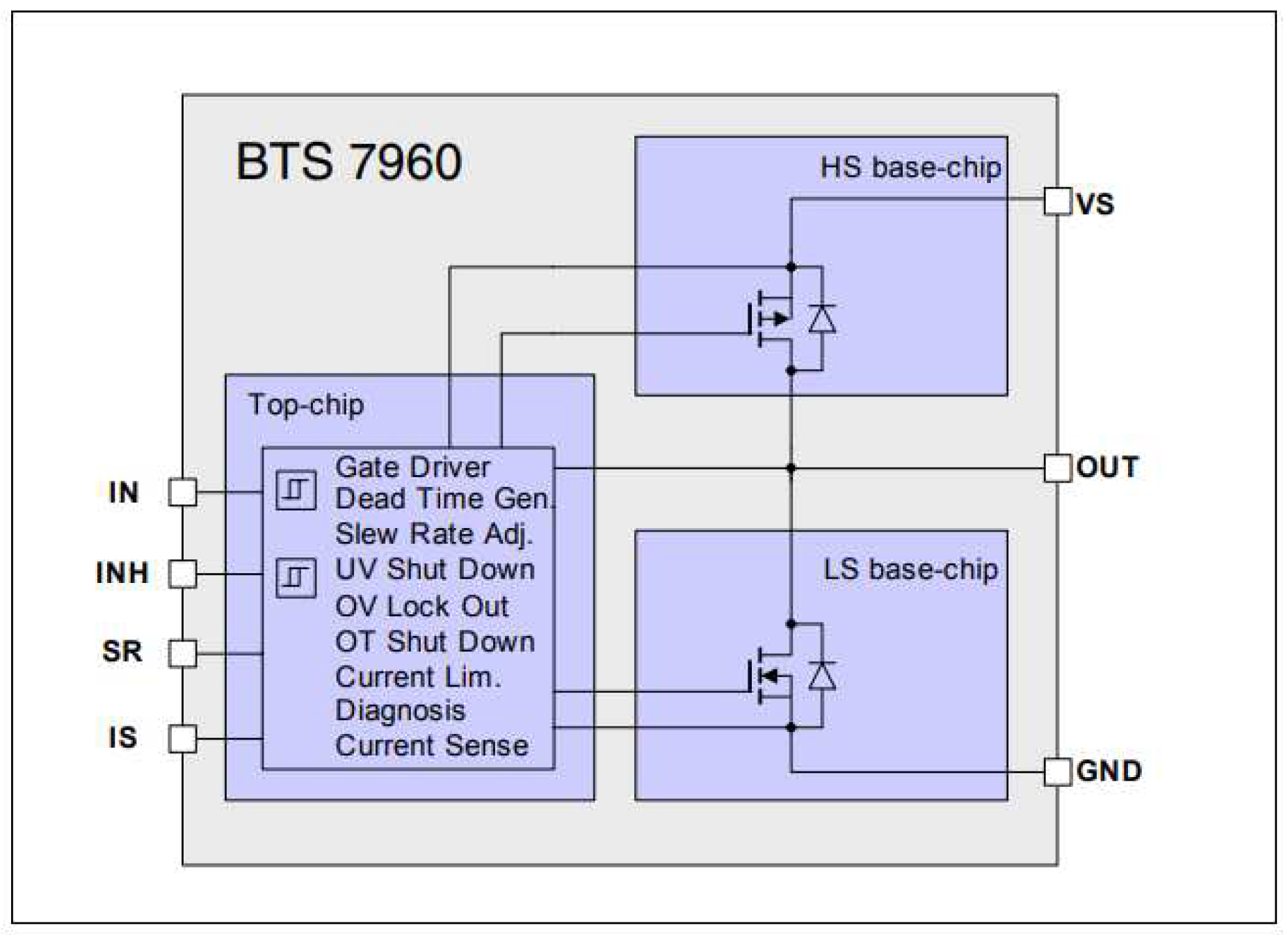
\{\begin{matrix} T_{n} = T_{1}, \\ T_{i} = 2 K_{1} T_{t o t}, \\ K_{p} = T_{n} / T_{i}, \\ T_{i} = 1 / T_{i} . \end{matrix}

To rotate the motors, it was used three BTS7960 microcircuits (Figure 8), each of which contains two MOSFET transistors forming a half-bridge, as well as the logic necessary to control it, including a built-in dead time generator, protection from overloads, short circuits, high supply voltage, which makes their integration, and also increases the reliability of the finished device. The permissible supply voltage of the microcircuits is up to 27 volts, and the switching current is up to 40 amperes.

An absolute encoder qy3806 is used for feedback to the motor interaction with it occurs via the SPI interface.

4.1. Drive systems

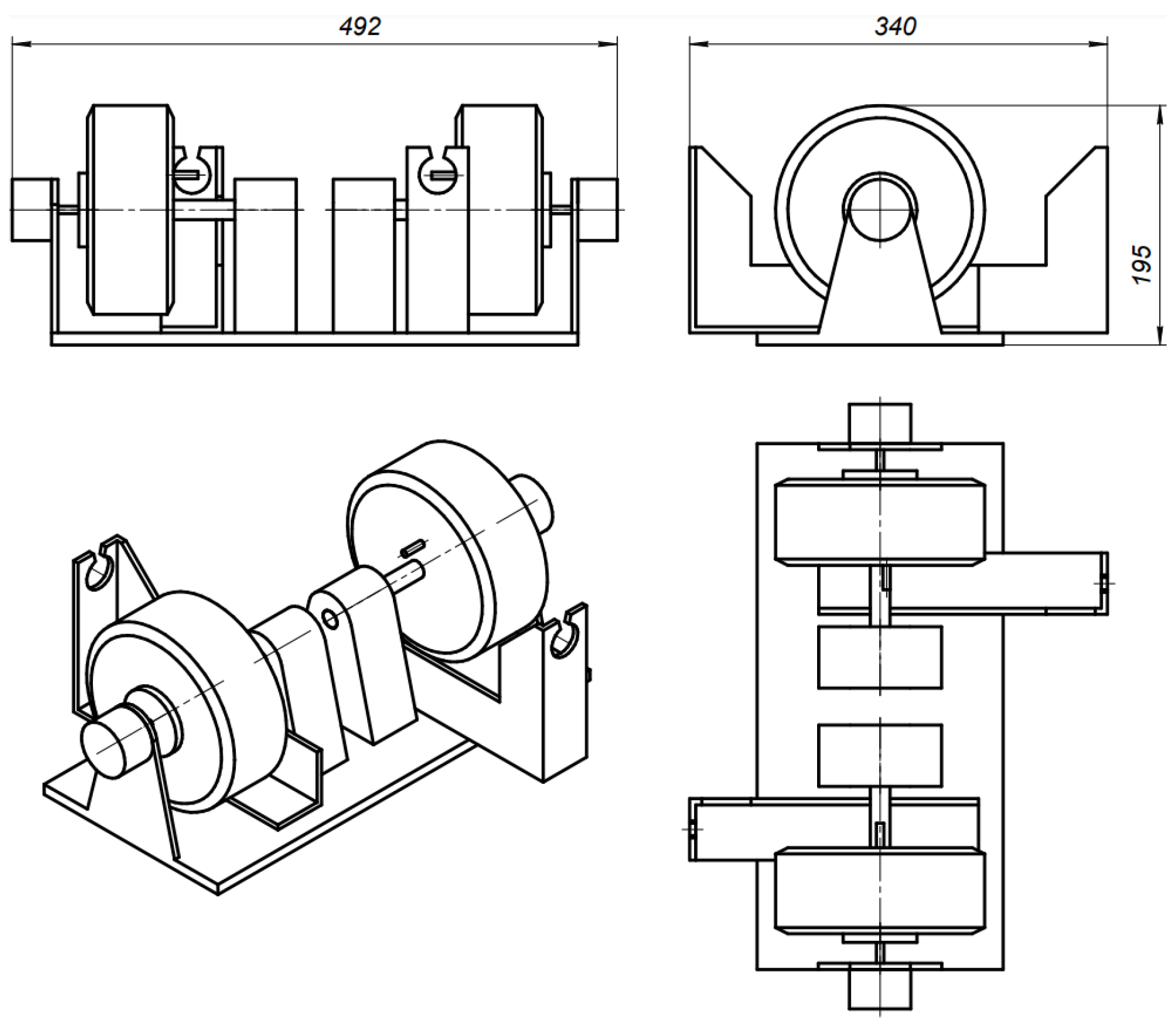
Besides electronic components, to develop an unmanned vehicle, the conversion kit must also include the drives themselves, which handle the movement of the vehicle control elements. Physical control of one brake pedal (the gas pedal is completely electronic), the gear selector, and the angle of rotation of the steering shaft are required in the HAV equipped with an automatic transmission. Thus, three drives are required, and it is convenient to combine the selector and brake drives into one remote module and place them in any convenient place in the HAV. The possibility of free placement of drives appears because of the use of special automotive cables: a regular one is sufficient for the brake pedal, but a pusher is required for the gearbox selector.

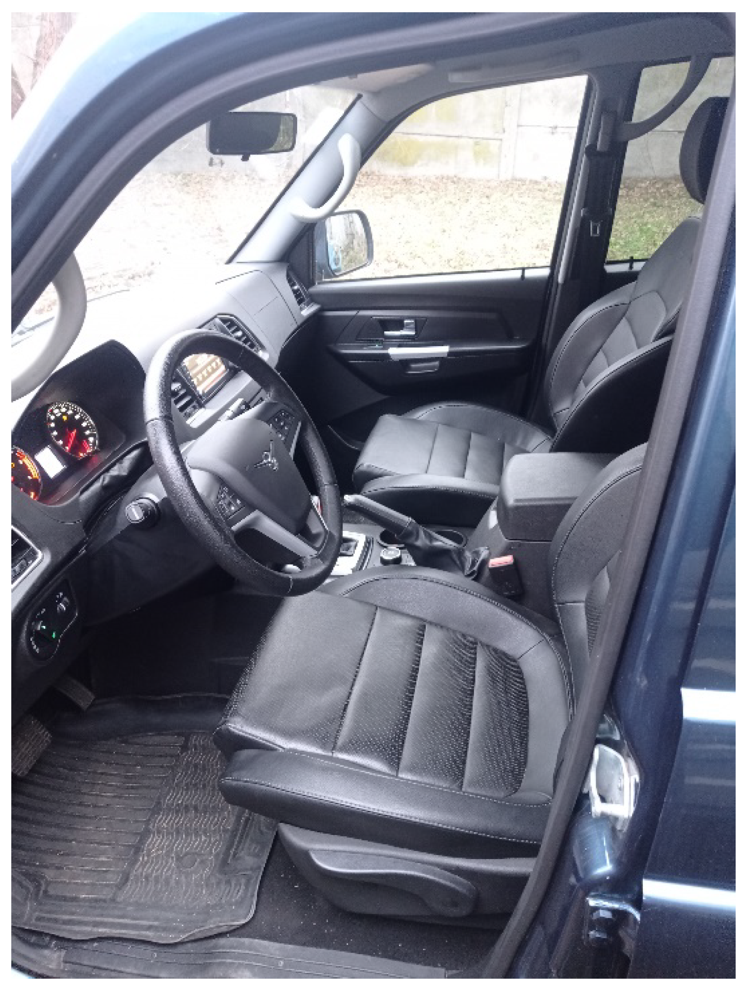
The possibility of unimpeded interception of control by the operator should be left in place when developing control systems for vehicle controls. Synchronous motors were used as motors instead of actuators for this purpose. A specific module was developed to control the brake and gearbox of a vehicle (Figure 9). Its peculiarity is the ability to install the device itself not only directly next to the controls, but for example under the seat or inside the trunk of the HAV, and because of the use of thin cables. It remains possible to close all the standard interior covers of the HAV, preserving the original condition of the HAV as much as possible (Figure 10).

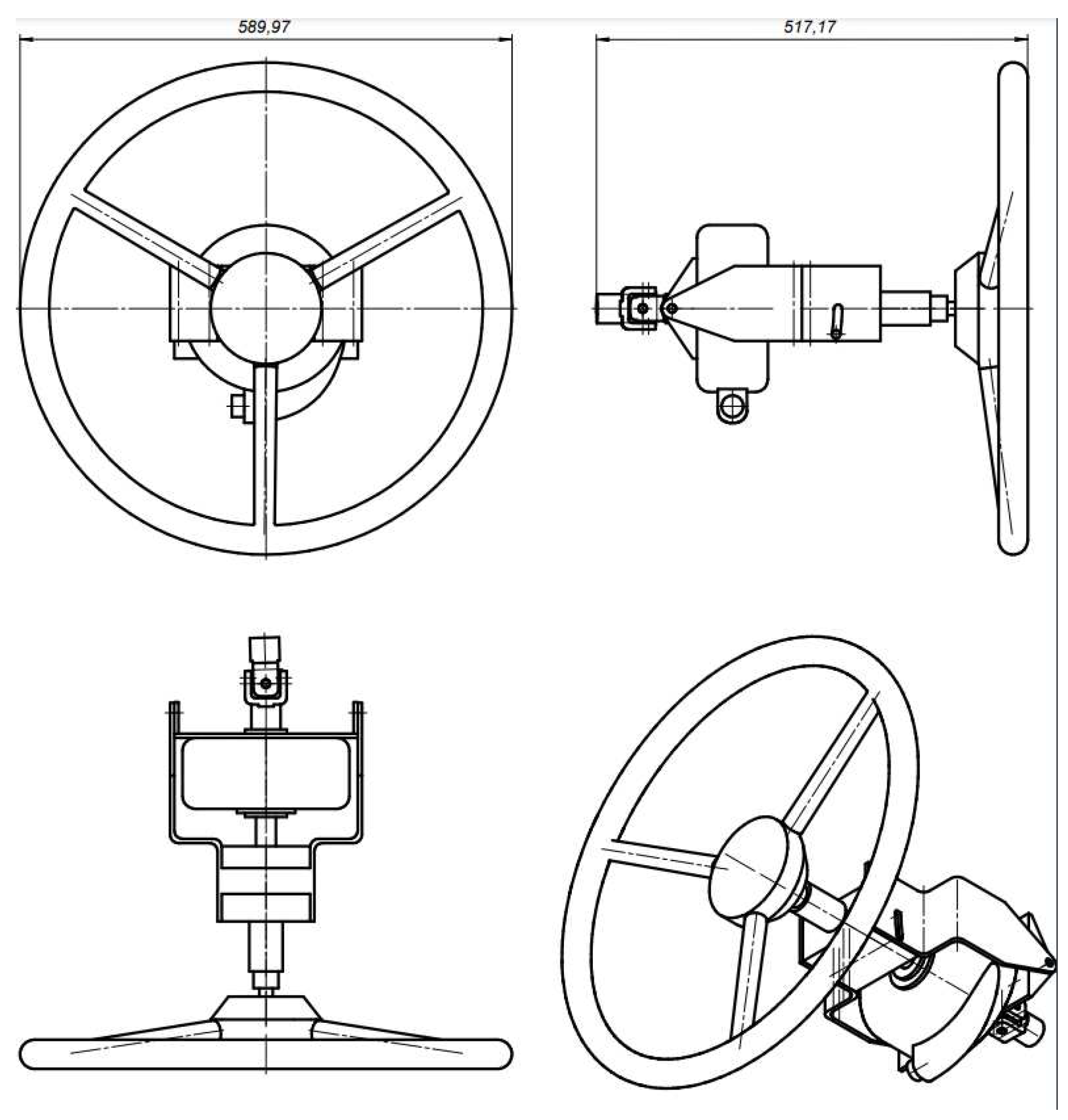
The steering of the HAV undercast significant modifications by integrating an additional motor that rotates the steering shaft, since most trucks and work vehicles are not equipped with factory electronic power steering. Module with a serial EMS2 drive to rotate the steering shaft was developed based on the standard UAZ Patriot steering column. The standard ability to adjust the steering wheel in height and reach is kept (see Figure 11).

5. Results of computational experiments

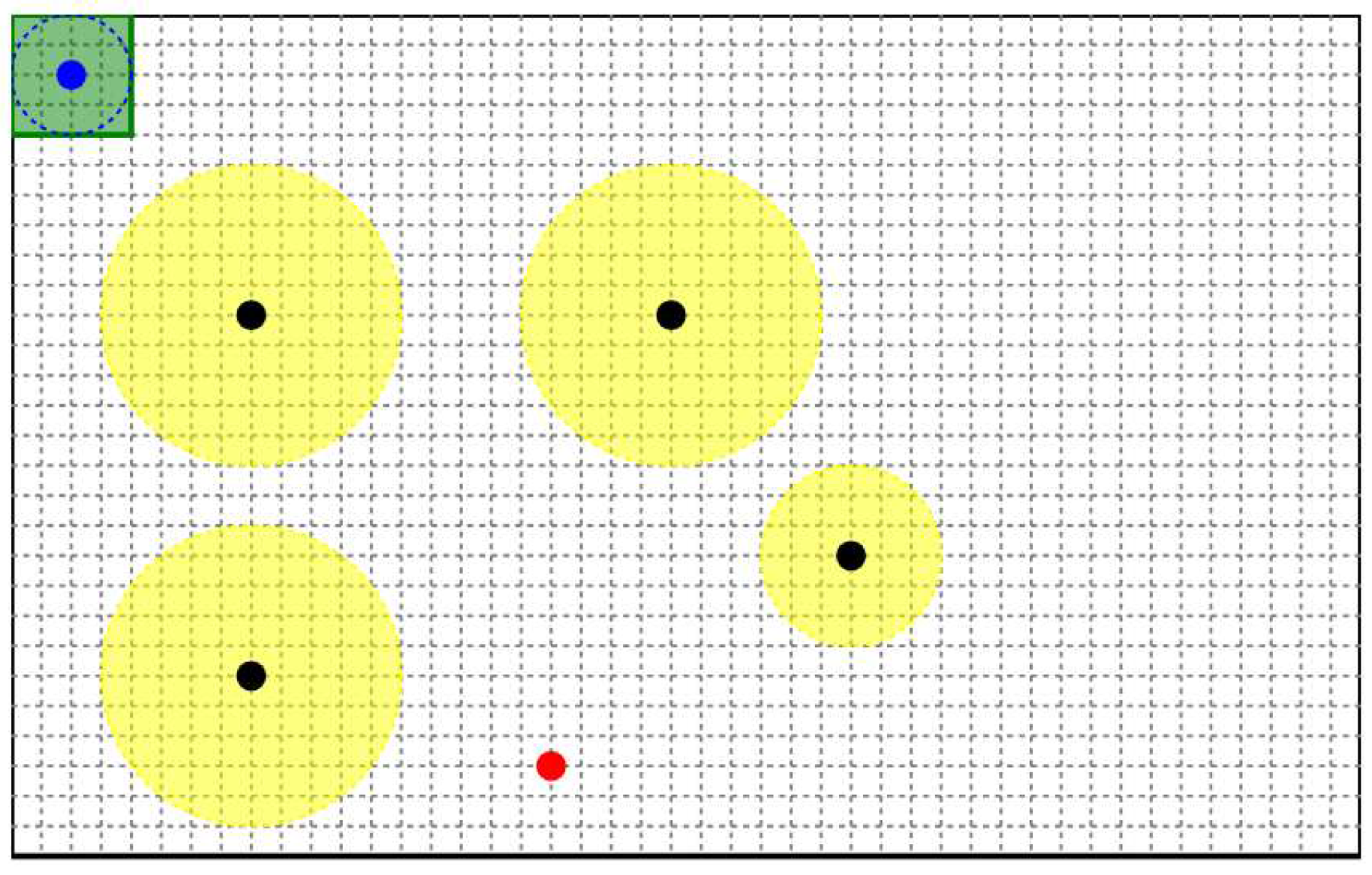
A modeling system has been developed to conduct computational experiments with proposed Q-learning algorithm as a web application in Python language [37] using the Flask framework. Matrix calculations were performed using the NumPy library. Figure 12 shows the main simulation window.

As you can see in Figure 1, a HAV model has initial coordinates (20,20). There are four obstacles in the simulated environment: three of them have a radius of 50 units, and one has a radius of 30 units. The grid size is 10 units. The dot at the bottom of the simulation window illustrates the final point of route that the HAV must reach. Modeling window size is 450 x 280 unit.

The results of all experiments which are presented in this article were conducted with the following algorithm parameters:

Learning rate is 0.1.
Reward discount factor is 0.9.
Penalty for going out of bounds is -10.
Penalty for enters an area marked as an obstacle is -100.
Penalty for passing the simulation environment field is -1.
Reward for finding the target is 100.
Probability of choosing a random action is 10%.

5.1. Experiment 1 (100 episodes)

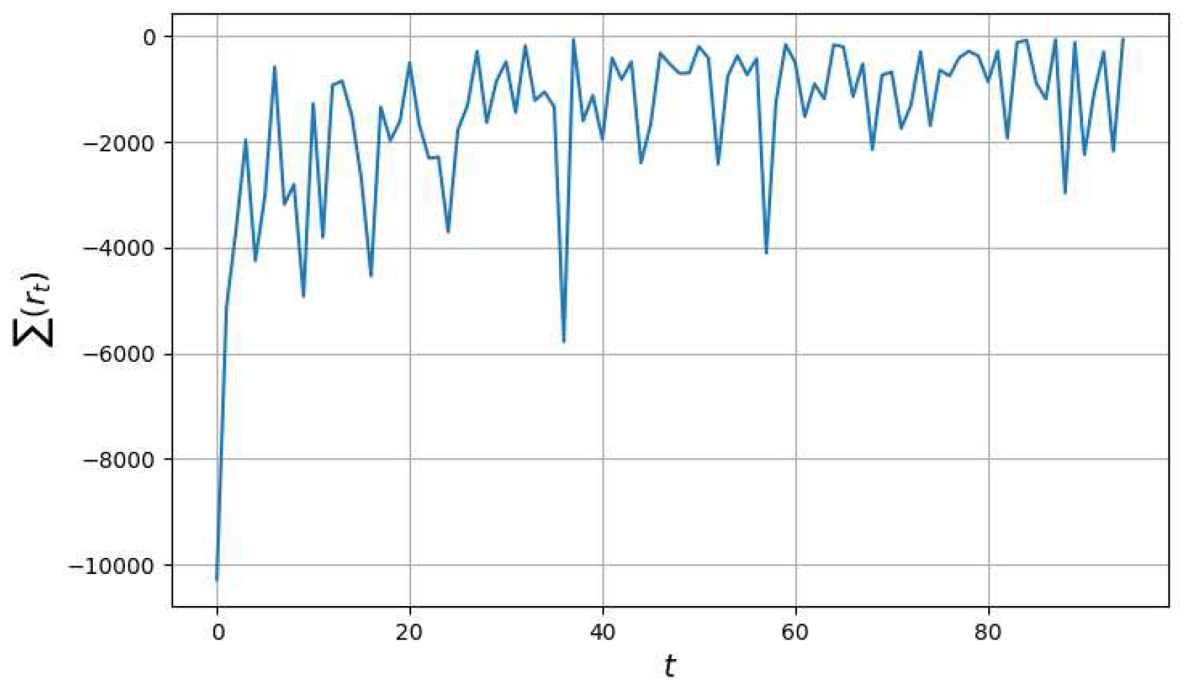
Figure 13 shows the graph of changes in the total reward when modeling the HAV trajectory for 100 episode. As you can see that the agent is undertrained and the trajectory contains random movements, which are often exploratory.

5.2. Experiment 2 (500 episodes)

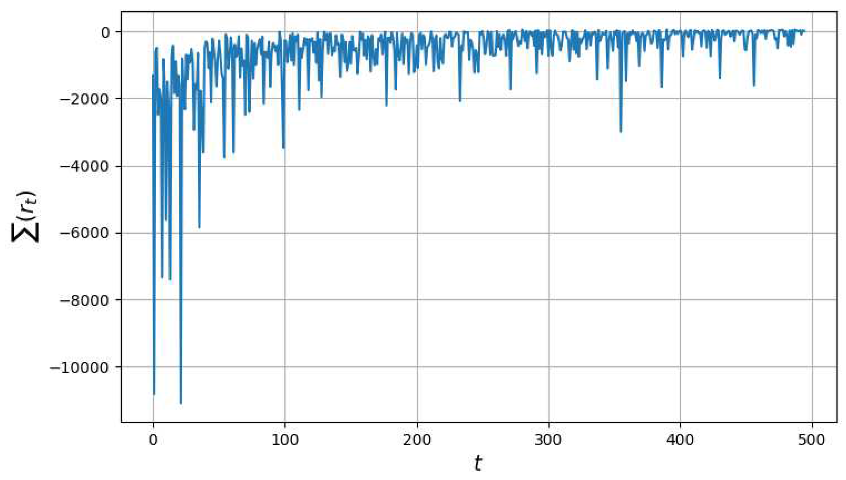
Figure 14 shows the graph of changes in the total reward when modeling the HAV trajectory for 500 episode. The trajectory of the HAV is more stable compared with the previous experiment, with few random movements.

As you can see in Figure 14, there is a convergence to the positive values of the total agent reward. However, there are still significant deviations from the optimal value.

5.3. Experiment 3 (1000 episodes)

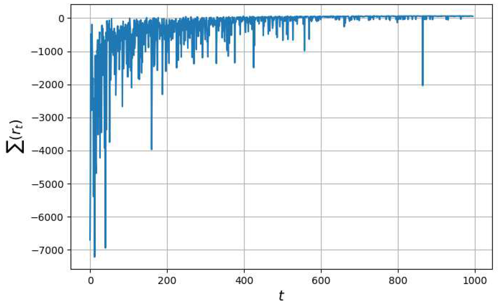
This experiment shows that training the algorithm on 1000 episodes is quite suffices to reach satisfactory results for a current task (Figure 15).

As you can see from Figure 15, there is a convergence to the positive values of the total agent reward with minimal deviations. The spike in the value of the total reward at approximately at episode 850 is associated with the random choice of the agent actions in 10% of decision-making.

6. Conclusions

This paper describes methods and tools for designing a HAV control system for movement along waypoints. The waypoint information of the HAV movement across the field is formed after executing the proposed Q-learning algorithm as a vector of points, each of which corresponds to a geographic coordinate.

The main advantage of the proposed approach is that the intelligent agent learns without having previously known information about the environment in which it is placed. It is shown that with a few number of states of the environment, convergence of the learning algorithm is observed.

The developed tools were tested in a simulation environment and in a real UAZ Patriot vehicle.

As the future work, authors will plan to develop path planning tools based on maps and a model of the surrounding scene.

Author Contributions

These authors contributed equally to this work. All authors have read and agreed to the published version of the manuscript.

Funding

This study was funded by Russian Science Foundation grant No. 23-11-00265, https://rscf.ru/project/23-11-00265/.

Data Availability Statement

Not applicable.

Acknowledgments

Authors are grateful for a GAZ, UAZ, SimbirSoft, Avion, ”Precision farming systems” and RITG companies.

Conflicts of Interest

The authors declare no conflict of interest. The founding sponsors had no role in the design of the study; in the collection, analyses or interpretation of data; in the writing of the manuscript, or in the decision to publish the results.

References

Xu, Jiaqi, Shengxiang She, Pengpeng Gao, and Yunpeng Sun. "Role of green finance in resource efficiency and green economic growth." Resources Policy 81 (2023): 103349. [CrossRef]
Liu, Liangkai, Sidi Lu, Ren Zhong, Baofu Wu, Yongtao Yao, Qingyang Zhang, and Weisong Shi. "Computing systems for autonomous driving: State of the art and challenges." IEEE Internet of Things Journal 8, no. 8 (2020): 6469-6486. [CrossRef]
Mier, Gonzalo, João Valente, and Sytze de Bruin. "Fields2Cover: An open-source coverage path planning library for unmanned agricultural vehicles." IEEE Robotics and Automation Letters 8, no. 4 (2023): 2166-2172. [CrossRef]
Christiaensen, Luc, Zachariah Rutledge, and J. Edward Taylor. "The future of work in agriculture: Some reflections." World Bank Policy Research Working Paper 9193 (2020). [CrossRef]
EvoCargo official site. — URL: https://evocargo.com/ (accesed: 28.11.2023).
Komatsu, Tomohiro, Yota Konno, Seiga Kiribayashi, Keiji Nagatani, Takahiro Suzuki, Kazunori Ohno, Taro Suzuki, Naoto Miyamoto, Yukinori Shibata, and Kimitaka Asano. "Autonomous driving of six-wheeled dump truck with a retrofitted robot." In Field and Service Robotics: Results of the 12th International Conference, pp. 59-72. Springer Singapore, 2021. [CrossRef]
Flämig H. Autonomous Vehicles and Autonomous Driving in Freight Transport // Autonomous Driving / Maurer M., Gerdes J., Lenz B., Winner H. (eds). — Springer, Berlin, Heidelberg, 2016. [CrossRef]
Sviatov, Kirill, Nadejda Yarushkina, Daniil Kanin, Ivan Rubtcov, Roman Jitkov, Vladislav Mikhailov, and Pavel Kanin. "Functional Model of a Self-Driving Car Control System." Technologies 9, no. 4 (2021): 100. [CrossRef]
Omeiza, Daniel, Helena Webb, Marina Jirotka, and Lars Kunze. "Explanations in autonomous driving: A survey." IEEE Transactions on Intelligent Transportation Systems 23, no. 8 (2021): 10142-10162. [CrossRef]
Montanaro, Umberto, Shilp Dixit, Saber Fallah, Mehrdad Dianati, Alan Stevens, David Oxtoby, and Alexandros Mouzakitis. "Towards connected autonomous driving: review of use-cases." Vehicle system dynamics 57, no. 6 (2019): 779-814. [CrossRef]
Sviatov, Kirill, Nadejda Yarushkina, Daniil Kanin, Ivan Rubtcov, Roman Jitkov, Vladislav Mikhailov, and Pavel Kanin. "Functional Model of a Self-Driving Car Control System." Technologies 9, no. 4 (2021): 100. [CrossRef]
OpenStreetMap Homepage. URL: http://openstreetmap.ru (acessed: 28.11.2023).
Hildebrandt, Florentin D., Barrett W. Thomas, and Marlin W. Ulmer. "Opportunities for reinforcement learning in stochastic dynamic vehicle routing." Computers & operations research 150 (2023): 106071. [CrossRef]
LaValle, Steven. "Rapidly-exploring random trees: A new tool for path planning." Research Report 9811 (1998).
Zhao, Jiuxia, Minjia Mao, Xi Zhao, and Jianhua Zou. "A hybrid of deep reinforcement learning and local search for the vehicle routing problems." IEEE Transactions on Intelligent Transportation Systems 22, no. 11 (2020): 7208-7218.
Peng, Bo, Jiahai Wang, and Zizhen Zhang. "A deep reinforcement learning algorithm using dynamic attention model for vehicle routing problems." In Artificial Intelligence Algorithms and Applications: 11th International Symposium, ISICA 2019, Guangzhou, China, November 16–17, 2019, Revised Selected Papers 11, pp. 636-650. Springer Singapore, 2020. [CrossRef]
Zheng, Shi. "Research on the Bias Sampling RRT Algorithm for Supermarket Chain Distribution Routes under the O2O Model." Frontiers in Computing and Intelligent Systems 5, no. 2 (2023): 52-55.
Ramadhan, Fadillah, and Arif Imran. "An adaptation of the record-to-record travel algorithm for the cumulative capacitated vehicle routing problem." In 2019 IEEE International Conference on Industrial Engineering and Engineering Management (IEEM), pp. 238-242. IEEE, 2019. [CrossRef]
Sutton, Richard S., Marlos C. Machado, G. Zacharias Holland, David Szepesvari, Finbarr Timbers, Brian Tanner, and Adam White. "Reward-respecting subtasks for model-based reinforcement learning." Artificial Intelligence 324 (2023): 104001. [CrossRef]
Graesser, Laura, and Wah Loon Keng. Foundations of deep reinforcement learning. Addison-Wesley Professional, 2019.
Busoniu, Lucian, Robert Babuska, and Bart De Schutter. "A comprehensive survey of multiagent reinforcement learning." IEEE Transactions on Systems, Man, and Cybernetics, Part C (Applications and Reviews) 38, no. 2 (2008): 156-172. [CrossRef]
Yang, Lin, and Mengdi Wang. "Reinforcement learning in feature space: Matrix bandit, kernels, and regret bound." In International Conference on Machine Learning, pp. 10746-10756. PMLR, 2020.
Watkins, Christopher JCH, and Peter Dayan. "Q-learning." Machine learning 8 (1992): 279-292. [CrossRef]
Millán-Arias, Cristian, Ruben Contreras, Francisco Cruz, and Bruno Fernandes. "Reinforcement Learning for UAV control with Policy and Reward Shaping." In 2022 41st International Conference of the Chilean Computer Science Society (SCCC), pp. 1-8. IEEE, 2022. [CrossRef]
Choi, Ji-wung, Renwick Curry, and Gabriel Elkaim. "Path planning based on bézier curve for autonomous ground vehicles." In Advances in Electrical and Electronics Engineering-IAENG Special Edition of the World Congress on Engineering and Computer Science 2008, pp. 158-166. IEEE, 2008.
Dubins, Lester E. "On curves of minimal length with a constraint on average curvature, and with prescribed initial and terminal positions and tangents." American Journal of mathematics 79, no. 3 (1957): 497-516. [CrossRef]
Reeds, James, and Lawrence Shepp. "Optimal paths for a car that goes both forwards and backwards." Pacific journal of mathematics 145, no. 2 (1990): 367-393. [CrossRef]
Sutton, Richard S., David McAllester, Satinder Singh, and Yishay Mansour. "Policy gradient methods for reinforcement learning with function approximation." Advances in neural information processing systems 12 (1999). [CrossRef]
Kim, Jong Min, Kyung Il Lim, and Jung Ha Kim. "Auto parking path planning system using modified Reeds-Shepp curve algorithm." In 2014 11th International Conference on Ubiquitous Robots and Ambient Intelligence (URAI), pp. 311-315. IEEE, 2014. [CrossRef]
SAE Levels of Driving Automation. URL: https://www.sae.org/blog/sae-j3016-update (acessed: 28.11.2023).
Betz, Johannes, Tobias Betz, Felix Fent, Maximilian Geisslinger, Alexander Heilmeier, Leonhard Hermansdorfer, Thomas Herrmann et al. "TUM autonomous motorsport: An autonomous racing software for the Indy Autonomous Challenge." Journal of Field Robotics 40, no. 4 (2023): 783-809. [CrossRef]
Balaji, Bharathan, Sunil Mallya, Sahika Genc, Saurabh Gupta, Leo Dirac, Vineet Khare, Gourav Roy et al. "Deepracer: Autonomous racing platform for experimentation with sim2real reinforcement learning." In 2020 IEEE International Conference on Robotics and Automation (ICRA), pp. 2746-2754. IEEE, 2020.
Buehler, Martin, Karl Iagnemma, and Sanjiv Singh, eds. The 2005 DARPA grand challenge: the great robot race. Vol. 36. springer, 2007. [CrossRef]
Imran, Hamza Ali, Usama Mujahid, Saad Wazir, Usama Latif, and Kiran Mehmood. "Embedded development boards for edge-ai: A comprehensive report." arXiv preprint arXiv:2009.00803 (2020).
Automotive Ethernet: A Crossroads for the Connected Car. URL: https://embeddedcomputing.com/application/automotive/vehicle-networking/automotive-ethernet-a-crossroads-for-the-connected-car (accesed: 28.11.2023).
Strobl, Simon. "Field Oriented Control (FOC) of Permanent Magnet Synchronous Machine (PMSM)." imperix power electronics (2021): 1-9.
Ravichandiran, Sudharsan. Hands-On Deep Learning Algorithms with Python: Master deep learning algorithms with extensive math by implementing them using TensorFlow. Packt Publishing Ltd, 2019.

Figure 1. Example of the cubic Bezier curve.

Figure 2. Example of the Dubins curve.

Figure 3. Example of paths based on the Reeds-Shepp and Dubins curves.

Figure 4. Basic elements of an simulation environment:

s_{0}

is an agent initial state;

S t

is an obstacle.

Figure 4. Basic elements of an simulation environment:

s_{0}

is an agent initial state;

S t

is an obstacle.

Figure 5. Example of proposed simulator work.

Figure 6. Example of the proposed algorithm work.

Figure 7. Architecture of the HAV command execution subsystem.

Figure 8. Block diagram of BTS7960.

Figure 9. Drawing of a device with drives for the gearbox and brake pedal.

Figure 10. Refurbished interior of a UAZ Patriot.

Figure 11. Drawing of a modified steering column with thruster.

Figure 12. Main simulation window.

Figure 13. Changes in total reward value over 100 episodes.

Figure 14. Changes in total reward value over 500 episodes.

Figure 15. Changes in total reward value over 1000 episodes.

Table 1. Q-table example.

	$a_{1}$	$a_{2}$	$a_{3}$	$a_{4}$
$s_{1}$	$q_{*} (s_{1}, a_{1})$	$q_{*} (s_{1}, a_{2})$	$q_{*} (s_{1}, a_{3})$	$q_{*} (s_{1}, a_{4})$
$s_{2}$	$q_{*} (s_{2}, a_{1})$	$q_{*} (s_{2}, a_{2})$	$q_{*} (s_{2}, a_{3})$	$q_{*} (s_{2}, a_{4})$
$s_{3}$	$q_{*} (s_{3}, a_{1})$	$q_{*} (s_{3}, a_{2})$	$q_{*} (s_{3}, a_{3})$	$q_{*} (s_{3}, a_{4})$
$s_{n}$	...	...	...	...

Table 2. Example of a completed Q-table.

	down	up	left	right
(20,20)	9,8	-1,4	7	4,3
(20,30)	1,6	4,1	0	4,8
(30,30)	7,7	5,2	7	3,3
(30,40)	6,3	5,6	8	1,1

Disclaimer/Publisher’s Note: The statements, opinions and data contained in all publications are solely those of the individual author(s) and contributor(s) and not of MDPI and/or the editor(s). MDPI and/or the editor(s) disclaim responsibility for any injury to people or property resulting from any ideas, methods, instructions or products referred to in the content.

© 2023 by the authors. Licensee MDPI, Basel, Switzerland. This article is an open access article distributed under the terms and conditions of the Creative Commons Attribution (CC BY) license (http://creativecommons.org/licenses/by/4.0/).

Copyright: This open access article is published under a Creative Commons CC BY 4.0 license, which permit the free download, distribution, and reuse, provided that the author and preprint are cited in any reuse.

MDPI Initiatives

Important Links

Choose an area of interest and we will send you notifications of new preprints at your preferred frequency.

Disclaimer

Approach of Trajectory Generation Based on Waypoint Information for a Highly Automated Vehicle

Abstract

1. Introduction

2. Related works

2.1. Algorithms for generating HAV movement waypoints

2.2. Algorithms for constructing a trajectory based on waypoints information

3. Proposed approach

3.1. Q-learning algorithm for generating HAV trajectory waypoints information

3.2. Algorithm for trajectory generation based on waypoint information and Reeds-Shepp curves

4. System architecture and circuit solutions

4.1. Drive systems

5. Results of computational experiments

5.1. Experiment 1 (100 episodes)

5.2. Experiment 2 (500 episodes)

5.3. Experiment 3 (1000 episodes)

6. Conclusions

Author Contributions

Funding

Data Availability Statement

Acknowledgments

Conflicts of Interest

References

MDPI Initiatives

Important Links

Subscribe