
Submitted:
29 November 2023
Posted:
29 November 2023
You are already at the latest version
Abstract
Two pre-pulses focused at different positions and at different time moments were used to enhance THz emission generated by the main pulse. The emission of THz radiation from air breakdown regions of focused ultrashort fs-laser pulses (800 nm/35 fs) at shockwave front prepared by pre-pulses was investigated, and a 3D spatio-temporal control was established for the most intense emission. The laser pulse-induced air breakdown forms a ~120 micrometers-long focal volume and generates a shockwave that delivers denser air into the focal region of the main pulse for enhanced generation of THz radiation at 0.1-2.5 THz spectral window. The intensity of pre- and main-pulses was at the tunneling ionisation intensities (1-3)x1016 W/cm2 and corresponded to sub-critical (transparent) plasma in air. Polarisation analysis revealed that the orientation of the air density gradients generated by pre-pulses and their time-space placement defined the ellipticity of the generated THz electrical field. The rotational electric current is the origin of THz radiation. The current is created by non-parallel gradients of electron density and temperature. Scaling dependencies of THz emission control are established.
Keywords:
THz radiation
; femtosecond laser-induced breakdown
; air breakdown
; spatiotemporal control
; coupling of temperature
; density gradients in plasma
; tunnelling ionisation
1. Introduction
High-intensity ultra-short laser pulses become inseparable from the future development of industrial applications in 3D nano-/micro-machining/printing due to Moore’s law-like increase of their average power over the last years from 2000 [1]. Deterministic energy deposition via highly nonlinear multi-photon and avalanche ionisation is key to 3D CNC machining metals and dielectrics from TW/cm2 to PW/cm2 intensity window [2]. The laser ablation thresholds in the case of ultra-short 10 - 50 fs pulses attracted interest due to better control of laser machining depth and removed volume as observed in dielectrics [3], however absent in metals [4]. For example, in fused silica SiO2, the ablation threshold was 1.3 J/cm2, i.e., 1.5 times smaller than for longer fs-pulses, and the most efficient rate of ablated volume per pulse was at 4 J/cm2 fluence or 0.57 PW/cm2 intensity for 7 fs pulses [3]. Formation of an over-critical (reflective) plasma mirror at the central part of the Gaussian intensity profile defined energy deposition efficiency and high precision ablation depth control with tens-of-nm per pulse. The ablated volume per energy saturates at the 30 fs pulse duration. Plasma mirror is proposed for compression of ultra-short laser pulses to reach the exawatt intensity scale [5]; 1 EW = W.
A 3D printing/polymerisation at ∼TW/cm2 becomes ionisation controlled, and absorption defines polymerisation rather than the chemical composition of photo-initiators and two-photon absorbers. Deterministic energy deposition occurs at higher intensities corresponding to the tunnelling ionisation of molecules and atoms at PW/cm2 [6]. In ambient air, focusing ultra-short pulses of a few tens of fs into spots of a few micrometres in diameter is possible by reflective optical elements, which deliver intensities sufficient for the tunnelling ionisation [7]. Such conditions were explored in this study for THz radiation using instantaneous air breakdown along pulse propagation throughout the focus, which was sub-wavelength for emitted THz radiation.
THz spectral range THz (3 mm - 10 m in wavelength) has fundamental importance for material science due to characteristic lattice vibrations of phonon modes. Among established semiconductor-based THz emitters/receivers working on photo-activated optically gated currents (Auston switch), a new emerging direction is using nano-thin topological insulators [8]. Another emerging direction is the use of dielectric breakdown as a tool to create short-lived ( ps) and micro-localized (sub-wavelength at THz frequencies) currents for THz emission [9]. Coherent directional emitters at far-IR wavelengths can be realised using Wolf’s effect, where surface sub-wavelength structures of period m for far-IR black body radiation are defined to extract emission of the surface phonon polariton (SPP) mode at an angle from the normal to the crystal surface according to the phase matching condition for wavevectors along the surface: [10]. In this way, acoustic/optical photon THz frequencies are extracted into free-space radiation, which is, additionally, coherent due to the sub-wavelength character of the grating.
The single-cycle high-intensity of electrical THz field of 1 MV/cm was demonstrated with fs tilted-front pulses using optical rectification in LiNbO3 crystal [11]. Periodically polled lithium niobate was used to produce THz emission via walk-off of optical pump and THz wave [12]. High THz pulse energy of 10 J at a peak field strength of 0.25 MV/cm, was produced by optical rectification when phonon-polariton phase velocity was matched with the group velocity of driving fs-laser pulse and reached high visible-to-THz photon conversion of 45% [13]. Tunable 10-70 THz emitters were realised via difference-frequency mixing of two parametrically amplified pulse trains from a single white-light seed in GaSe or AgGaS2 crystals and reached 100 MV/cm peak field at W peak power (19 J energy) using table-top laser system [14]. Such high powers are usually produced by free electron lasers (FELs). The THz radiation is related to fast electrical current as per the Fourier transform, i.e., 1 ps current generates 1 THz radiation. Spin-Hall currents in tri-layers of 5.8-nm-thick W/Co40Fe40B20/Pt were used as THz broadband 1-30 THz emitters generating field strength of several 0.1 MV/cm and outperformed ZnTe emitters [15]. An electrical conductivity induced via the Zenner tunneling can be harnessed to induce electrical transients in semiconductors and dielectrics by strong optical fields. When an optical field of 170 MV/cm was applied to the Auston switch with a 50 nm gap on SiO2 by sub-4 fs pulse of 1.7 eV light, the currents were detected due to induced electron conductivity of 5 m−1, which is 18 orders of magnitude higher than the static d.c. conductivity of amorphous silica [16]. Optical control of phonon modes and Zenner tunneling can be operated without the dielectric breakdown maintaining solid-state material. High-intensity ultra-short irradiation of gasses, liquids, and solids at higher intensities, when the dielectric breakdown occurs, can also be used for producing high-intensity THz fields [17]. By co-propagation of the first and second harmonics beams focused with mm lens into long filaments in air plasma, the AC-bias conditions, THz emitters were realised delivering peak intensities up to 10 kV/cm [18,19,20]. Polarisation of the emitted THz radiation can be set circular by introducing non-colinearity between the filaments [21]. Irradiation of He-jet in vacuum was shown to produce coherent THz emission via the transition radiation of ultra-short electron bunches produced by the laser wakefield, which, in turn, was produced by 8 TW peak power pulses of 800 nm/50 fs [22]. The short length of the electron bunch was responsible for the coherent emission. The field of THz sources has become an active research frontier [23,24,25].
Here, we used a focused fs-laser pulse for air breakdown from sub-wavelength volumes, which can potentially lead to the engineering of high-intensity THz emitters due to the coherent addition of THz electrical fields and ultra-short duration of a few optical periods. Two pre-pulses used in this study revealed a position dependence on the THz emission and its polarisation, extending from the previous study where one pre-pulse was used [26]. Experimental conditions of focusing and THz detection were kept the same [26], and only two pre-pulses were introduced using a holographic beam shaping technique based on a spatial light modulator (LC- SLM) [27]. For consistency, the same pulse energies were used for pre- and main-pulses: 0.2 and 0.4 mJ (13 GW/pulse), respectively [26]. The range of THz emission was THz [26]. The experimental results were interpreted with a theoretical model accounting for the air ionisation and free electron heating, generation and propagation of a shockwave, and spontaneous generation of the magnetic field due to coupled thermal and density gradients at the shock front. Interestingly, two- or three-pulse irradiation with air breakdown and shock formation is approaching the frequencies THz of 5G network GHz (Technical Specification Group Radio Access Network TS 38.104).
2. Experimental results
Two-pulse experiment with pre- and main pulses [26] revealed the required timing and spatial separation for the shocked-compressed air by the pre-pulse to be pushed into the position of the main pulse at for the maximum emission of THz radiation. Pre-pulse had to arrive 9.7 ns earlier to the focus of the main pulse from the position m away for the maximum THz emission. Polarisation of THz radiation was found aligned along the direction of focal positions of pre-pulse and main pulse [26]. Here, we add a second pre-pulse of the same 0.2 mJ energy with the possibility of placing it freely in 3D space . Figure 1 shows the scheme of the experiment and the diagnostics. Details of the experimental setup and the measurement methodology are described in 6. The effect of placement of the second pre-pulse on polarisation and intensity of THz radiation was systematically studied. Due to short 35 fs pulse (m in length) and z-position (along the beam propagation) change only tens-of-micrometers. Hence, the timing of both pre-pulses can be considered simultaneous, regardless of the actual z-coordinate of the pre-pulse 2 within an error of nm, which is by an order of magnitude smaller than the shockwave thickness.
2.1. Y-position of pre-pulse 2
Figure 2 shows the emission of THz radiation ( component) for the situation when the pre-pulse 1 is focused at m. At the same time, the second pre-pulse is focused at other position with respect to the main-pulse focus at ; see Figure 1. Change of field orientation was observed over the measured range of THz frequencies as shown by the time domain transients in Figure 2(a). When two pre-pulses were simultaneously irradiated at opposite (with respect to ) positions, the cancellation of THz components occurred. This confirms that the air density gradient induced by the shock front is more important than the air mass density, which is increased by two colliding shocks.
For two pre-pulse experiments, a dependence of THz emission on the offset of the second pre-pulse was determined. The delay of the first pre-pulse of 9.7 ns was optimised, so the THz emission was the most intense. The THz intensity is calculated from the components as peak-to-peak value (see inset in Figure 3). A pictorial diagram for each irradiation point is presented by the projection of THz E-field on -plane. The projection shows the overall temporal evolution of THz electric field orientation during emission time.
One pre-pulse produced enhancement of THz emission by 13 times, i.e., the value V2 compared to the value V2 without a pre-pulse. The component of the THz field becomes larger for offsets m compared to the enhancement produced by the first Conversely, when pre-pulse 2 was closer to the position where the main pulse is focused, the amplitude of THz field was reduced.
The second pre-pulse of four times smaller energy of 0.05 mJ, had no significant effect on the THz emission, regardless of the position at , opposite side from pre-pulse 1 with respect to the main pulse focus. A different evolution in time for such 0.05 mJ second pre-pulse was observed. It showed a ps duration of larger negative values of component (see inset in Figure 3(c) and colour asymmetric markers). This is probably due to a later arrival and shorter contribution of a shock wave triggered by a four times lower pre-pulse energy. Indeed, the radius R of a cylindrical shock wave created by the laser energy deposition on the axis increases with time t as according to the Sedov–von Neumann–Taylor model [28]. The major contribution to the THz enhancement was governed by the first pre-pulse with an energy of 0.2 mJ.
Interestingly, when pre-pulse 2 was on the same side as pre-pulse 1 at a distance from the main pulse position larger than 33 m (pre-pulse-1), the enhancement was times (see Sec. Sec. 3 for discussion). In this case, the shock-affected volume from the pre-pulse 1 was crossed by the pre-pulse 2. When a shock wave propagates through a region of rarefied density formed by the other pre-pulse, the same cylindrical explosion model predicts scaling . When pre-pulse 2 arrived at to m (the opposite side of the y-axis as compared to pre-pulse 1), it quenched the effect of THz enhancement. However, at even more negative positions of pre-pulse 2, the same enhancement was observed for arriving shocks to the position of the main pulse; see red-dashed lines drawn as eye guides in Figure 3(c).
2.2. X-position of pre-pulse 2
Next, the dependence of THz emission of the x-position of the second pre-pulse was determined, see Figure 4. The trajectories indicate the radial influence of the pre-pulse irradiation position with respect to the main pulse (the pre-pulse 1 was always at the m). The ellipticity of THz polarisation was larger for the pre-pulse 2 locations (larger ). This is explained by the optimal timing of 9.7 ns for the pre-pulse position at m from the main pulse position. This is valid along any direction perpendicular to beam propagation in the plane. When m, the shock arriving along the x-axis does not fit the perfect timing for THz enhancement and alters the effect of the pre-pulse 1 arriving along a perpendicular direction. When m, pre-pulse 2 makes a small contribution to the enhancement determined by pre-pulse 1. The pre-pulses 1 and 2 arriving at perpendicular directions define the ellipticity of the THz radiation and its handedness (see Figure 4). The duration of the most intense THz radiation lasts approximately one cycle, corresponding to rotation in the plane (see a side-view cross-section along the time axis in the inset of Figure 4).
The dependence of THz emission on the position of the pre-pulse along the Z axis is presented in B.
3. Theoretical description of light-air interaction and THz emission
3.1. Laser air ionization and electron heating
Here, a physical scenario of air breakdown by the pre-pulse and main pulse and the dynamics of the plasma formation are analysed. The laser pulse parameters, the air ionisation potentials and the main experimental results are summarised in C.
Laser focusing in our experiment was carried out with an off-axis parabolic mirror with an effective numerical aperture as determined from direct imaging of water-jet breakdown [29]. The focal spot area is estimated from the Airy disk radius m, which is close to optical observation by shadowgraphy at low pulse energies. The axial extension of the air breakdown zone in the experiment is m [26]. It is close to the depth-of-focus , where the Rayleigh length m. The focusing volume is considered as a cylinder of length , radius and volume cm3.
The energy of the pre-pulse mJ and the main-pulse mJ correspond to the intensity W/cm2 and W/cm2, respectively. Under these conditions, the laser ponderomotive potential is much larger than the ionization potential of atoms, the air is ionised in the tunnelling regime, and a plasma is created in the focusing volume.
The plasma creation is estimated for the air consisting of 20% of oxygen and 80% of nitrogen molecules. The ionization rate as a function of laser electric field and atomic charge i is taken according to the Ammosov-Delone-Krainov (ADK) theory [30]. For the sake of simplicity, we assume a consecutive ionization from unperturbed atomic levels.
Electron ionization and heating are described by the kinetic equation for the distribution function of free electrons, , where is the electron partial distribution function corresponding to the atom ionization from the level j:
where is normalized by the density of neutral atoms, , is the laser electric field, is the probability of ionization from the level j, is the delta function and is velocity. In the case of linear polarization, non-relativistic electric field, and neglecting electron collisions, the electrons are moving in the direction of the laser field, and the distribution function is one-dimensional.
This equation describes the production of free electrons and their energy increase. The energy is taken from the laser field; therefore, the laser absorption and atom ionization proceed simultaneously. Integrating kinetic equation, one obtains equations for the three moments of electron distribution function, , and :
These equations are solved numerically for each ionization level and each atom separately, and the average ionization and the average residual electron energy are evaluated as
Two examples of numerical solutions are shown in Figure 5 for (left) and for the main pulse and the nitrogen atom. The electron residual energies are on the order of ionisation potential and significantly smaller than the ponderomotive energy. This is in agreement with the theoretical analysis [31].
The total ionisation energy per atom (assuming 80% nitrogen + 20% oxygen), the number of free electrons per atom, and the residual average electron energy are: for the pre-pulse eV, , and eV; for main pulse eV, , and eV. Multiplying the total energy loss per ion, , by the ion density and the focal volume, we obtain the free electron density and the laser energy loss for ionisation and electron heating. For the pre-pulse propagating in the air at normal conditions, the electron density is cm−3 and the energy loss is J. For the main pulse, considering propagation along the shock front in air compressed by a factor , the electron density is cm−3 and the laser energy loss is J.
3.1.1. Laser collisional absorption
In addition to the ionisation energy loss, the laser pulse transfers its energy to electrons due to the electron-ion collisions. As it is a weaker effect, we account for it as an addition to ionisation using standard expressions for the electron collision frequency and Coulomb logarithm [32]:
where the is the electron density in cm−3 and electron temperature is in eV. For estimates of the collision frequency during the laser pulse, we take the electron ponderomotive energy instead of ; after the end of the laser pulse, the isotropisation is fast, and we take as the two-thirds of the residual electron energy.
For the pre-pulse, the electron collision frequency ps−1, and the fraction of laser energy lost is 0.4%, which corresponds to the electron energy gain of J. For the main pulse, assuming that air is compressed 5.4 times, the electron collision frequency ps−1, the fraction of laser energy lost is 7.2% and the electron energy gain is J.
Combining the ionisation energy, residual electron energy, and collisional heating for the pre-pulse, we estimate the total energy loss of J, electron density cm−3 and electron temperature of 26.6 eV. Collisional heating contributes about 10% to the electron temperature at the end of the laser pulse. The electron collision frequency is 72.6 ps−1, so isotropisation proceeds very rapidly after the end of the laser pulse.
For the main pulse, the total absorbed laser energy is J, the electron density is cm−3, and the electron temperature is 64.1 eV. Collisional heating contributes about 23% to the electron temperature at the end of the laser pulse. The electron collision frequency is 147.4 ps−1.
3.2. Propagation of the heat wave and shock formation
After the laser pre-pulse, the thermal energy in plasma is J. It is larger but comparable to the shock energy measured in the experiment. The plasma pressure is 9.3 kbar. It leads to plasma expansion and the formation of a cylindrical shock on a time scale of a few hundred ps. According to the measurements [26], the shock propagates a distance of m in 10 ns, and the air compression in the shock front is , which is slightly less than the maximum compression for the air adiabat .
The parameter that defines the shock formation is where cm2/s is the electron heat conductivity, and km/s is the sound velocity. (See details of derivation in D). The shock formation time is 650 ps, and the initial shock position is m. The initial shock velocity is km/s, which corresponds to the Mach number . These values are the initial conditions for the cylindrical shock that can be described by the Taylor-Sedov formula: . The Mach number decreases as a square root of time.
The thickness of the shock front is needed for further analysis of mechanisms of electromagnetic emission. A general theory of shock waves predicts the front width on the order of a few molecule mean free paths [28]. A more detailed analysis [33] of the shock in air evaluates the front thickness as mean free paths for the shock Mach number . The mean free path of a molecule in air at normal conditions is m. Consequently, we take the shock front thickness m as a reference value.
The authors of ref. [34] have reported on the studies of shock excitation in air under conditions similar to our experiment. They used a 0.5 PW/cm2, 360 fs pulses at 1030 nm wavelength focused by objective lens and showed initiation of air breakdown along m long focus. A shock wave formation started 0.1 ns after the shot. The experimentally determined threshold intensity of the air breakdown was 80 TW/cm2. Experimental results of shock wave propagation are well fitted by the equation of state of air , where is the internal energy per unit volume, which is driving explosion. Initial pressures reaching kbar level were reduced to tens of bar after propagation of a few micrometers; the Mach number and velocity of shock wave were determined from a side view imaging. This paper also shows that a tighter focusing can localise the shocked region to small volumes within cross-sections of tens-of-m [34] and are promising for sub-wavelength sources of THz radiation. These conditions are similar to our study.
3.3. Diffusion currents
Since the electromagnetic emission is produced on a time scale larger than the electron collision time, the electron inertia can be neglected, and Ohm’s law describes the current excitation after the end of the laser pulse:
where the first term on the right-hand side describes the electric resistivity due to electron collisions, , and the second term represents the source related to the gradient of the electron pressure .
The main laser pulse propagates parallel to the shock front (along the z-axis) and perpendicular to the direction of shock wave propagation (the x-axis). The density profile in the shock front is asymmetric: it has a fast rise at the front side and a slow decrease at the rear side.
The electron temperature is also inhomogeneous; it is larger on the laser axis and decreases with the radius in the plane perpendicular to the laser propagation direction. Since the electron density and temperature gradients are non-parallel, the electric current has two components: an electrostatic component in the direction of the pressure gradient and a rotational component, which generates a magnetic field perpendicular to the density and temperature gradient. These currents are considered in the next two sections.
3.3.1. Electrostatic diffusion current.
The electrostatic current is associated with the charge density perturbation described by the continuity equation . Inserting in this equation expression for the current from Eq. (5) and using the Poisson equation for the electric field, , we obtain the following equation for the electron density:
where is the electron diffusion coefficient and is the electron plasma frequency. This equation describes the generation of an electrostatic field due to the diffusion of electrons heated by the laser pulse, which is similar to the photo-Dember effect in semiconductors [35,36]. Before the laser pulse arrival, the air is neutral. The laser pulse creates free electrons and heats them. Under the pressure gradient, the electrons start moving, while the ions are left behind because of their large mass. Therefore, the electron mobility creates an electric current, which induces the charge separation and electric field. Eventually, the electron diffusion stops when the pressure gradient is compensated by the electrostatic field.
We neglected in Eq. (6) excitation of plasma oscillations assuming that the time of electron heating equal to the laser pulse duration (about 30 fs) is much longer than the plasma wave period, , which is about 3 fs. The value of the charge separation, , is estimated by comparing the second term on the left-hand side, with the term on the right-hand side. The value of charge separation is , where is the electron Debye length. Since the Debye length in the experiment is on the order of 1 nm, about two orders of magnitude smaller than the shock front thickness, the charge separation of very small, about four orders of magnitude smaller than the plasma density. Therefore, Eq. (6) can be linearized and written for :
The second term on the right-hand side drives the charge separation because the diffusion coefficient increases with time during the laser heating. The first term on the right-hand side accounts for the charge relaxation due to collisions. This time is much shorter than the laser pulse duration. So, the time derivative on the left-hand side can be neglected; that is, the charge separation is almost instantaneously accommodated to the laser heating and . The strength of the saturated electric field is MV/cm is quite large, but no current is created.
This analysis confirms that electron diffusion cannot produce electromagnetic emission in the experiment.
3.3.2. Rotational diffusion current.
The mechanism of generation of the rotational component of electric current is illustrated in Figure 6. It is called the Biermann battery effect [37,38] in plasma physics. The crossed gradients of temperature and density induce a rotational electric current, which is not related to the charge separation and evolves on a longer time scale. The current is related to the magnetic field by Ampere’s equation, . The equation for the magnetic field is obtained by taking the curl of Ohm’s equation (5) and using Faraday’s equation for the curl of the electric field:
(We assume here a constant resistivity.) Since the gradients of the temperature and density on the right-hand side are in the plane, the diffusion proceeds in that plane, and only z-component of the magnetic field is generated.
The characteristic time of magnetic field generation, , is found by comparing the two terms in the left-hand side of this equation. The value of the magnetic field after the saturation is estimated by comparing the second term on the left-hand side with the term on the right-hand side: , and the estimate of the current follows from the Ampere equation: .
Equation (8) is solved numerically by considering a Gaussian distribution for the temperature, , and an exponential density profile, created at . The coordinate origin corresponds to the axis of the main pulse. The magnetic field is approximated in the polar coordinates as where describes the radial profile of magnetic field:
The left panel in Figure 7 shows the dependence of the dimensionless function on the radius and time. The magnetic field increases linearly with time for , and then it is saturated at the level . The radial profile has a maximum at . The spatial distribution of the magnetic field in the plane perpendicular to the laser propagation direction is shown in the right panel in Figure 7. It has a dipole structure with a positive lobe for and a negative lobe for . So, the average magnetic field is zero. The lines of constant magnetic field correspond to the current streamlines. The current is directed along the x direction near the axis, and the current loops are closed. An approximate analytical expression for the magnetic field is given in E.
For the parameters of the main pulse and for the air compression 5.4, we find the diffusion time ps, the maximum value of the magnetic field T and the maximum current density GA/cm2. The lifetime of that current and magnetic field is limited by heat diffusion. It is evaluated in the preceding section to be on the order of a few hundred ps. Performing integration over the focal volume for , we obtain the energy of the magnetic field after the saturation: . For our parameters, the total magnetic energy is about J. This sets the upper limit of the emitted electromagnetic energy.
3.4. Electromagnetic emission
Electromagnetic emission can be deduced from the general formula for the vector potential induced by the time-dependent current,
where is the delayed time. Considering the radiated field in the far field zone, , where is the unit vector in the emission direction, and performing the Fourier transform in time, we have then the following expression for the vector potential
where is the Fourier component of the current and is the wave number of emission. Since the emission zone is smaller than the wavelength of emission, , we develop the exponent under the integral in Taylor series, , and the terms in this series correspond to multipole expansion.
The terms and do not contribute to the radiation because and also . The first relation is evident since the current is a derivative of magnetic field: and . The second relation is obtained by integrating by parts the left-hand side and knowing that the integral of the magnetic field over y is zero. Thus, a non-zero contribution comes from the quadrupole term , which is written as:
where is the unit vector in the laser propagation direction, and is the Fourier component of magnetic field . The integral over the magnetic field at the source can be performed using the analytic approximation for the magnetic field (A6). Taking then a curl of the vector potential, we have the magnetic field in the far field zone:
where is the Fourier component of the time-dependent factor in Eq. (A6). The last factor accounts for the suppression of the emission because of a small ratio of the emission zone to the emission wavelength, .
Knowing the magnetic field in the far field, we calculate the electric field as and obtain the emission power in the solid angle :
Integrating the emission power over time, we obtain the total emitted energy. Using the theorem of Parceval, we replace the integral over time with the integral over frequency and obtain the spectrum of emission:
In the spherical coordinate system with the polar axis along the z direction and azimuthal angle in the plane with respect to the x axis, we have and , so the angular dependence of the emission power is
Since both electric and magnetic fields are proportional to , the maximum of emission is in the y direction. The polarization is in the direction; that is, the polarization is perpendicular to the observation direction in the plane defined by the observation direction and the x axis. The function under the integral represents the emission spectrum:
Divergence of the spectrum at high frequencies is due to the discontinuity in the time dependence of the magnetic field at time corresponding to the shock ionization by laser and electron heating. There are several options to introduce the switch-on time of the magnetic field generation: the laser pulse duration, the electron collision time, and the time of laser pulse propagation along the focal volume. Among the three options listed above, the longest one is the latter: ps. Since the integral over the spectrum is dominated by the cut-off frequency , corresponding to the cut-off wavelength of m and frequency of 5 THz.
Integrating the emission power over the angles and spectrum, we obtain the total emitted energy:
Comparing the radiated energy with the energy stored in the magnetic field in the focal zone, , the factor defines the emission efficiency. For the magnetic field energy of J, the radiated energy is 81 pJ, and the radiation power is about 400 W. That estimation is about four times larger than the measured emitted energy of 22 pJ, which can be considered as a reasonable agreement.
4. Discussion
The theoretical estimates for the frequency cut-off and the emitted energy are compatible with the observations. The analytical expressions for these parameters show the way of further improvements. The conversion efficiency of the magnetic field into radiation can be increased either by increasing the ratio with a tighter laser beam focusing or by creating a non-zero average magnetic field in the plasma. This will increase the conversion efficiency by a factor of . The structure of the magnetic field given by Eq. (A6) corresponds to the circular laser beam interacting with a planar shock. To produce a non-zero average magnetic field one may consider an elliptic laser beam with the ellipse axis at an angle (not equal to 0 or 90°) with respect to the x axis.
Another possibility of increasing emission consists of increasing the magnetic field energy. According to the analysis of Eq. (8), the generated magnetic field depends effectively on two plasma parameters: electron temperature and shock front width . The magnetic field energy depends on electron temperature with the fifth power. So, even a modest increase in electron temperature by a factor of 1.5 will increase the emission energy by 10 times. This can be achieved by increasing the energy of the main laser pulse.
In conclusion, the theoretical analysis of THz emission in air with two laser pulses confirms the hypothesis proposed by Huang et al. [39] that the emission is produced from a plasma created by the main pulse in the shock front. The theoretical estimates of the plasma and shock parameters are in agreement with the measurements. However, the mechanism of electromagnetic emission is different from the diffusion current in semiconductors [36]. An electrostatic current related to the charge separation cannot be excited in plasma. Instead, a rotation current is created by non-parallel gradients of electron density and temperature. This current induces a magnetic field and produces a magneto-quadrupole electromagnetic emission. The emission wavelength is controlled by the length of the laser focal region and can be varied by changing the numerical aperture.
5. Conclusions and Outlook
By using two pre-pulses with the same timing at focal spots placed at different 3D locations with respect to the focus of the main pulse, it is possible to engineer air density gradients arriving at the main irradiation site. An addition of two perpendicular air density gradients and allows one to control the ellipticity and intensity of the emitted THz radiation. A single cycle circular polarisation THz radiation can be produced. By placing m-diameter focal spots in 3D space with separations of in space and ns in time, it is possible to synchronise the arrival of shock wave fronts travelling at high Mach m/ns speeds in the air for THz emission enhancement and polarisation control at the laser pulse intensities of a fully deterministic tunnelling ionisation W/cm2.
The origin of THz emission is the current induced at the crossed plasma density and temperature gradients, called the Biermann battery effect [38]. This study clarified that the electrostatic current related to the charge separation cannot be excited in plasma. A coalescence of two shocks at the position of the main pulse produces stronger air compression than a single pulse, thus generating a stronger THz emission at a shorter wavelength. Since the electron current is proportional to the electron temperature and inversely proportional to the shock thickness, the way to increase the power of THz emission would be the increase of electron temperature and the strength of the shock.
After the collision of two shocks created by two pre-pulses, the interaction of the main laser pulse with the compressed air creates a plasma with asymmetric density distribution, which affects the intensity and polarisation of the THz emission in a two-fold way. First, the three-dimensional density asymmetry produces the anisotropy of pressure force and permits the current circulation on a picosecond time scale. Second, the shock density gradient is defined by the angle of collision of two shocks created by two pre-pulses. It is not necessarily aligned along the line connecting the pre-pulse and the main pulse, which affects the polarisation of the THz signal. The privileged direction of THz emission is in the plane perpendicular to the laser pulse propagation. This is the theoretical prediction that is verified in the experiment.
An example of a high-density micro-target for the generation of an extreme UV emission at 13.5 nm for the next generation of photolithography is realised by irradiation of 20-m diameter Sn micro-spheres by a focused 10 m wavelength CO2 laser [40]. Similarly, micro-jets of Ga produced by laser pulse showed a strong enhancement of X-ray generation [41]. In water, micro-droplets and micro-sized gradients of compressed air serve the same purpose of delivering more material into laser pulse/beam, which results in plasma with higher density and temperature [42,43].
6. Materials and Methods
All the experiments were conducted in air under atmospheric pressure (1 bar) at room temperature (RT; 296 K). The experimental setup is described in detail elsewhere [29]. A pulsed femtosecond laser (35 fs, transform-limited, nm, 1 kHz, Mantis, Legend Elite HE USP, Coherent, Inc.) was used and the output pulses were split into the pre-pulse 1 (linearly-polarized parallel to the y-axis, y-pol., 0.2 mJ), pre-pulse 2 (linearly-polarised parallel to the y-axis, y-pol., 0.2 mJ) and the main pulse (linearly-polarized parallel to the x-axis, x-pol., 0.4 mJ). THz emission is induced by tightly focussing the main pulse with an off-axis parabolic mirror (1-inch diameter, focal length mm, 47-098, Edmund Optics) into air with a time-delay, ns, between the main pulse and the pre-pulse arrivals. Under the main pulse focusing condition with effective numerical aperture , the laser focus area was estimated to be about m in diameter and m in length along the axial direction (depth-of-focus) [29].
Spatial offsets of the two pre-pulses along the x- and y-axes, and , were made possible with a Liquid Crystal on Silicon-Spatial Light Modulator (LCOS-SLM, X15213, Hamamatsu Photonics). The homemade program used computer-generated holograms (CGHs) that form multiple focal points and display them on the LCOS-SLM. CGHs were optimized by the weighted Gerchberg-Saxton (WGS) algorithm [44] for the uniform intensity of the focal points. The pre-pulse 1 was set stationary at (, , ) = (m, m, m) while the pre-pulse 2 was scanned in three dimensions along the x-, y-, or z-axis using 3D holographic focusing [45].
The detection of the THz wave emission is achieved by the standard electro-optic sampling method (see A), THz time-domain spectroscopy (THz-TDS), in the transmission direction along the z-axis with a -oriented ZnTe crystal (1-mm thick, Nippon Mining & Metals Co., Ltd.) [9,29,46]. The measurements of the THz polarisation were carried out with a set of wire grids before the detection -oriented ZnTe crystal following the standard procedure [47,48,49]. Both polarisations of the THz emission were determined from the event of laser irradiation by the main pulse via calculation of the measured fields using orientated wire-grid polarisers in respect to the x-polariser (high transmission) placed just before the polariser. The effective repetition of the laser excitation is at 0.5 kHz to restore the same air conditions for subsequent laser shots. Two laser pulses (main) were required to determine and components separately. Transient of THz emission was established from separate laser shots for the -5 to 15 ps -projections.
Acknowledgments
This research was funded by the National Science and Technology Council (NSTC, formerly known as MOST) of Taiwan 107-2112-M-001-014-MY3, 110-2112-M-001-054 (K.H. and H-H. H.) and partly funded by the Australian Research Council Linkage LP 220100153 grant (S.J.). We are grateful to Prof. Eugene G. Gamaly for the critical comments.
Appendix A. Electro-optical sampling
THz electric field strength [kV/cm] has to be measured or estimated in order to compare data between different experiments using a similar electro-optical (EO) sampling method. Two A and B channels of a balanced EO detector define the phase shift induced by the peak electric field of THz pulse in ZnTe crystal for the nm laser pulse [50,51]:
where [V] are the detector readouts (for A and B channels), is the refractive index of ZnTe at , pm/V is the electro-optical coefficient of ZnTe, and mm is the crystal length; the values listed are specific to our experiment. For calibration, the maximum amplitude of the EO-detector signal is measured [V] and corresponds to the incident optical power [W]; reflectance losses at normal incidence 12.3%. The EO-detector output in [V] is computed from optical powers [W] as , where the responsivity of the photo-detector (Model 2307) A/W at 800 nm and [V/A] (a low gain setting; for the high gain [V/A]) is the amplifiers trans-impedance gain. From Eq. (A1), [kV/cm]; here . For the main pulse of mJ, i.e., the measured average power of mW (at 1 kHz repetition rate) one finds [mW] [V]. With typical values of V (Figure 2), we find the [kV/cm] for the main pulse (in the case of two-pulse irradiation with the pre-pulse at 0.2 mJ in air and focus in -plane).
The measured voltages along -orientations using EO sampling were obtained from two measurements of the front linear polariser at orientations (see Figure 1). The while .
The maximum amplitude of was observed for a specific two-pre-pulse geometry with the placement of two pre-pulses in 3D space (Figure A2) and it was up to 4 times larger than for the one-pre-pulse case with the focal plane being -plane. With two pre-pulses of 0.2 mJ and a main pulse of 0.4 mJ it is possible to engineer polarisation and reach kV/cm at the optimised space-time localisation of the focal volumes of all three pulses.
Even 444 times larger fields can be produced by two-pulse irradiation of water micro-sheets (m) at the same experimental conditions: focusing, pulse energies and polarisations, positions of the focal regions [52]. This shows that production of MV/cm THz field strength using pure water flow is possible [42]. It is noteworthy, that the distance from the focal point of the main-pulse to the EO detector ZnTe was cm (Figure 1). The electrical field strength .
Figure A1.
Intensity of THz emission as a function of offsets along the z- and y-axes for the pre-pulse 2 (positions of the pre-pulse 1 m and main-pulse are fixed). Positive corresponds to the up-stream focal position of the pre-pulse 2 as compared with the main-pulse (and pre-pulse 1) and vice versa, the negative values are at the down-stream locations. The delay time between the pre-pulses and main pulse irradiation is 9.7 ns. The position of the first pre-pulse is at (m, m, m). Pre-pulse energies are 0.2 mJ and the main pulse is 0.4 mJ. The focal plane of main and pre-pulse 1 is marked at . See Figure A2 for the polarization projections at the same conditions as this intensity plot.
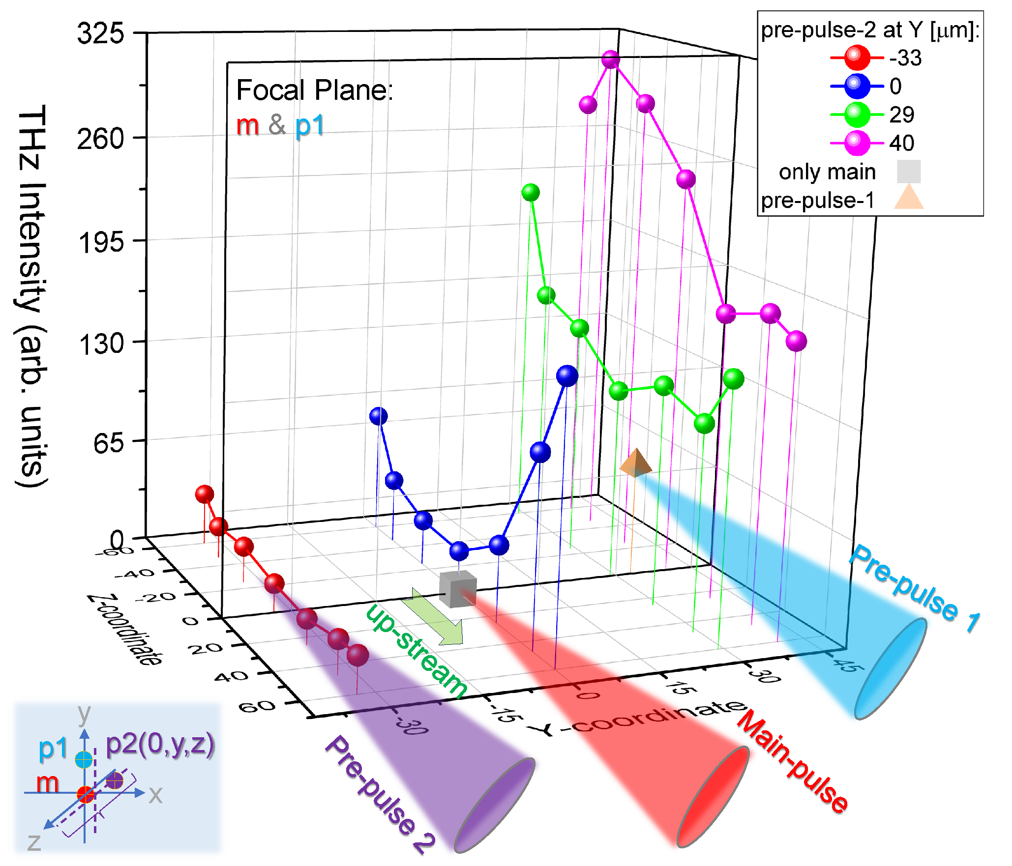
Figure A2.
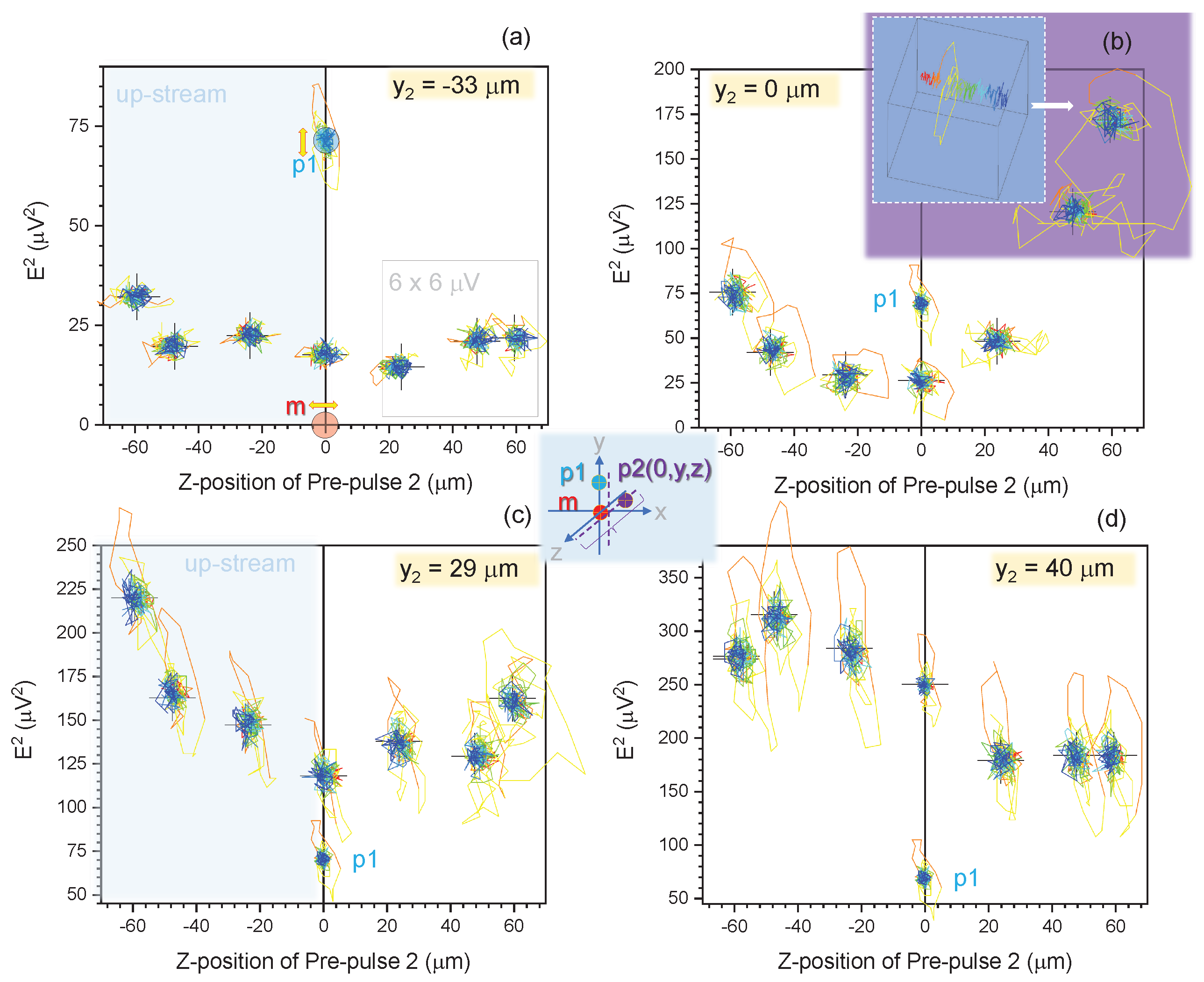
THz-polarization intensity as a function along the z-axis offset for the second pre-pulse at position m (a), 0 m (b), 29 m (c), 40 m (d) with for all cases, see the central inset for geometry of experiments. Positive corresponds to the up-stream focal position of the pre-pulse 2 as compared with the main-pulse (and pre-pulse 1) and vice versa, the negative values are at the down-stream locations. The delay time between the pre-pulses and the main pulse arrives at 9.7 ns. The spatial offset for the first pre-pulse irradiation is at (, , ) = (m, m, m). The marker p1 shows value for the 0.2 mJ pre-pulse 1 alone. The projection maps are all plotted on the same scale of V regardless of the scale of different panels (a-d) for .
Figure A2.
THz-polarization intensity as a function along the z-axis offset for the second pre-pulse at position m (a), 0 m (b), 29 m (c), 40 m (d) with for all cases, see the central inset for geometry of experiments. Positive corresponds to the up-stream focal position of the pre-pulse 2 as compared with the main-pulse (and pre-pulse 1) and vice versa, the negative values are at the down-stream locations. The delay time between the pre-pulses and the main pulse arrives at 9.7 ns. The spatial offset for the first pre-pulse irradiation is at (, , ) = (m, m, m). The marker p1 shows value for the 0.2 mJ pre-pulse 1 alone. The projection maps are all plotted on the same scale of V regardless of the scale of different panels (a-d) for .
Appendix B. Z-position of pre-pulse 2
The dependence of axial z-position of pre-pulses on THz generation is shown in Figure A1 for intensity only and for polarisation -map in Figure A2. Positive corresponds to the up-stream focal position of the pre-pulse 2 as compared with the main-pulse and pre-pulse 1; also vice versa, the negative values are at the down-stream locations. When second pre-pulse 2 is between m the location of the main pulse at m, the intensity of THz is quenched (Figure A2(a)); the pre-pulse 1 is at m (Figure 1). This is consistent with the results of Figs. Figure 2 and Figure 3, which showed that the gradient induced by shocks from pre-pulses 1 and 2 smear each other and reduce the intensity of THz radiation.
When pre-pulse 2 is focused at the position of the main pulse onto optical axis (and arrives later by 9.7 ns), there is also a reduction of the THz emission when the distance of pre-pulse 2 focus is less than m from , regardless up- or down-stream; see Figure A2(b). However, there is more than twice an enhancement in THz radiation when the focus of p2 is downstream by more than m. In this situation, ionisation of air along the optical axis acts as a back-reflector and was visualised in previous studies [26]. A single-cycle close to circularly polarised THz emission was observed for p2 focused at m see inset in (b).
When the pre-pulse 2 was irradiated at the upper -half-plane at positions m, the effect of THz emission was enhanced as compared with single pre-pulse 1 (Figure A1) as shown in Figure A2(c,d). For m, the 9.7 ns timing was close to two shock waves to reach the position of the main pulse (m) together, resulting in almost twice larger THz intensity. This addition is consistent with two gradients having major contributions along the same y-direction (c). A larger separation of p2 focus from resulted in a further increase of THz intensity (c,d).
Let us trace the polarisation changes of THz emission upon the z-position of pre-pulse 2. When two pre-pulses were on the same half of the -plane (), an elliptical polarisation of the overall THz emission was observed, and it became more linear (y-pol.) at the larger . The polarisation of the both pre-pulses is linear y-pol. (The main pulse is x-pol.). The same tendency of THz polarisation being y-linear is observed for one pre-pulse 1. For the case when both pre-pulses were on the opposite sides from to m locations, the polarisation of THz emission had a close-to-random polarisation (a). In this case, the air density gradients along the y-axis cancel each other; here are unit vectors of the Cartesian coordinates. For the case when p2 is scanned along the z-axis (propagation of the beam) at fixed position, the ellipticity of THz emission was increasing when a perpendicular contribution was added to the due to p1; also p2 was adding its own contribution. This vector nature of air density gradients was responsible for a complex polarisation of emitted THz radiation, which is discussed next.
Appendix C. Input parameters and experimental results for theoretical estimations
Here we summarise the laser input parameters and experimental results used in the theoretical analysis.
- Input parameters: laser is focused in the air at normal pressure cm−3. Nitrogen and oxygen are two-atom molecules, atomic density is .
- Laser pulse parameters: pulse duration fs, wavelength nm, repetition rate 1 kHz, focusing numerical aperture .
- Laser focusing zone: radius m, Rayleigh length m, cross-section area m2, and focal volume é cm−3.
- Pre-pulse energy 0.2 mJ: power 5.7 GW, flux 417 J/cm2, intensity W/cm2, ponderomotive energy eV.
- Main pulse energy 0.4 mJ: power 11.4 GW, flux 835 J/cm2, intensity W/cm2, ponderomotive energy 1446 eV.
- Potentials of ionisation of nitrogen: 14.6 eV, 29.6 eV, 47.5 eV, 77.45 eV, 97.9 eV.
- Potentials of ionisation of oxygen: 13.6 eV, 35.1 eV, 54.9 eV, 77.4 eV, 113.9 eV.
- For the pre-pulse, the probabilities of the ionisation of nitrogen are 1, 1, 1, 0.42, 0.007, and the residual energies are 0.95 eV, 23.9 eV, 45.0 eV, 77.5 eV, 58.4 eV. The probabilities of the ionisation of oxygen are 1, 1, 1, 0.43 and the residual electron energies are: 9.7 eV, 42.0 eV, 71.7 eV, 77.6 eV.
- For the main pulse, the probabilities of the ionisation of nitrogen are 1, 1, 1, 1, 0.93, and the residual energies are 14.2 eV, 27.3 eV, 51.2 eV, 134.8 eV, 153.0 eV. The probabilities of the ionisation of oxygen are 1, 1, 1, 1, 0.026 and residual energies are 11.3 eV, 48.2 eV, 84.2 eV, 134.5 eV, 127.3 eV.
- Experimental results. THz pulse is polarized linearly along the line connecting the two pulses. The spectrum maximum is at 1.5 THz, spectrum width is 1.5 THz. The maximum emission at the delay of 1.5 ns corresponds to m and maximum width of m; at 4.7 ns it is m and maximum width of m. Shock position is m at a time of 4.7 ns and m at 10 ns. Mach number is 19 at 1.5 ns, 9 at 4.7 ns and 6 at 9.7 ns. Sound velocity in air is 0.34 km/s. Compression is 5.6 at 4.7 ns and 5.2 at 9.7 ns. Photon number conversion efficiency is which is comparable with ZnTe crystal giving . Considering the ratio of wavelengths of laser to THz , the energy conversion efficiency is , that is, J or 22 pJ.
Appendix D. Propagation of the heat wave and shock formation
The shock is formed when the heat wave, which propagates radially from the laser-heated zone, is caught up by the acoustic wave. To characterize the shock formation, we need, therefore, to describe the propagation of the heat wave outside the focal volume. Assuming cylindrical geometry, we consider the heat wave propagating in the radial direction and described by the heat transport equation
where is the electron heat conductivity given by the Spitzer-Härm expression
This equation conserves the thermal energy released by the laser:
where is the initial temperature, is the position of the front of the heat wave, and is the radius of the heated zone.
Since the heat conductivity depends on the temperature as , the heat wave is nonlinear and, assuming a constant density, the temperature profile is described by a self-similar solution [28]:
where is the self-similar variable and the function satisfies the following differential equation:
The characteristic time of heat wave evolution is given by the relation: , where , and the solution is constrained by the condition of energy conservation
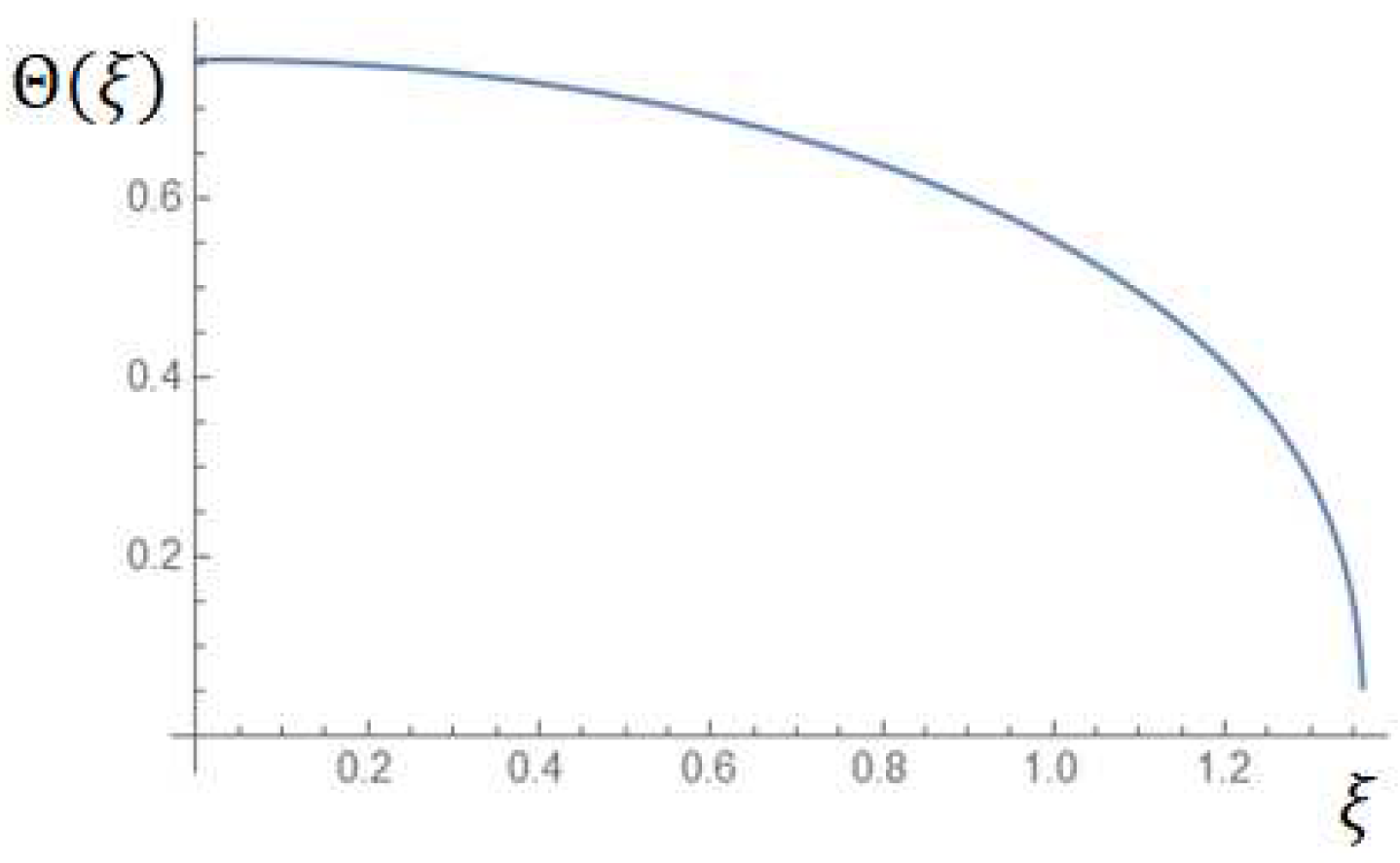
The solution of the equation for is shown in Figure A3. The value at the origin is , and the front position is . Consequently, the radius of the front is
This has to be compared to the position of the acoustic wave, which propagates with the velocity , it can also be written as , which corresponds to the adiabatic index 1, because of the plasma is quasi-isothermal. Since the temperature depends on time, the position of the acoustic wave is
It propagates faster than the thermal wave and catches it up when . This equation defines the time of shock formation, :
Using numerical values for the self-similar solution, the time of shock formation is
and the position of the shock front is
Figure A3.
Self-similar temperature profile.
Appendix E. Approximate solution for the magnetic field generated at the shock front
To simplify the calculations of THz emission, we approximate the magnetic field by separating the spatial and temporal dependence:
Figure A4.
Time (a) and radial (b) dependence of the magnetic field obtained from a numerical solution of Eq. (9) (solid lines) and the analytical approximation given by Eq. (A6).
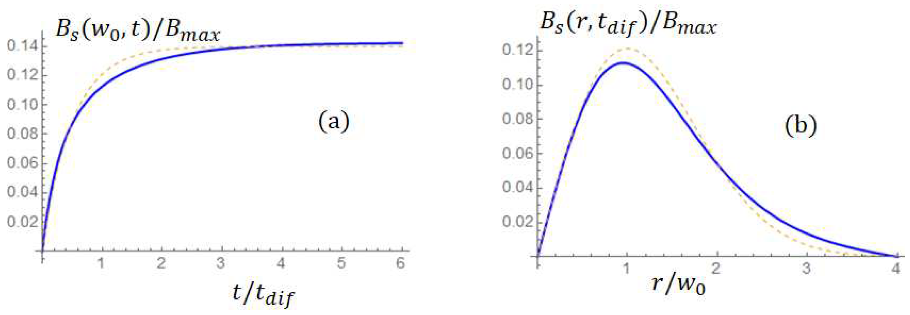
The quality of the approximation is shown in Figure A4 with two cuts at a constant r = w0 (a) and at a constant time t = tdif (b). In spite of small deviations, the approximation is in good agreement with the numerical solution.
References
- Han, M.; Smith, D.; Ng, S.; Anand, V.; Katkus, T.; Juodkazis, S. Ultra-Short-Pulse Lasers—Materials—Applications. Eng. Proc. 2021, 11, 44. [CrossRef]
- Mourou, G.; Tajima, T.; Bulanov, S. Optics in the relativistic regime. Rev. Modern Phys. 2006, 78, 309–371. [CrossRef]
- Utéza, O.; Sanner, N.; Chimier, B.; Sentis, M.; Lassonde, P.; Légaré, F.; Kieffer, J.C. Surface Ablation of Dielectrics with sub-10 fs to 300 fs Laser Pulses: Crater Depth and Diameter, and Efficiency as a Function of Laser Intensity. Journal of Laser Micro/Nanoengineering 2010, 5, 238–241. [CrossRef]
- Genieys, T.; Sentis, M.; Utéza, O. Measurement of ultrashort laser ablation of four metals (Al, Cu, Ni, W) in the single-pulse regime. Advanced Optical Technologies 2020, 9, 131–143. [CrossRef]
- Hur, M.; Ersfeld, B.; Lee, H.; Kim, H.; Roh, K.; Lee, Y.; Song, H.S.; Kumar, M.; Yoffe, S.; Jaroszynski, D.; Suk, H. Laser pulse compression by a density gradient plasma for exawatt to zettawatt lasers. Nature Photonics 2023, p. (online first). [CrossRef]
- Gibbon, P. Short Pulse Laser Interactions with Matter: an Introduction; Imperial College Press and distributed by World Scientific Publishing Co., 2005; [https://www.worldscientific.com/doi/pdf/10.1142/p116]. [CrossRef]
- Guo, L.; Han, S.S.; Liu, X.; Cheng, Y.; Xu, Z.Z.; Fan, J.; Chen, J.; Chen, S.G.; Becker, W.; Blaga, C.I.; DiChiara, A.D.; Sistrunk, E.; Agostini, P.; DiMauro, L.F. Scaling of the Low-Energy Structure in Above-Threshold Ionization in the Tunneling Regime: Theory and Experiment 2013. 110, 013001. [CrossRef]
- Kuznetsov, K.; Safronenkov, D.; Kuznetsov, P.; Kitaeva, G. Terahertz Photoconductive Antenna Based on a Topological Insulator Nanofilm. Applied Sciences 2021, 11, 5580. [CrossRef]
- Huang, H.H.; Nagashima, T.; Hsu, W.H.; Juodkazis, S.; Hatanaka, K. Dual THz Wave and X-ray Generation from a Water Film under Femtosecond Laser Excitation. Nanomaterials 2018, 8, 523. doi:10.3390/nano8070523. [CrossRef]
- Greffet, J.J.; Carminati, R.; Joulain, K.; Mulet, J.P.; Mainguy, S.; Chen, Y. Coherent emission of light by thermal sources. Nature 2002, 416, 61–64. [CrossRef]
- Hirori, H.; Doi, A.; Blanchard, F.; Tanaka, K. Single-cycle terahertz pulses with amplitudes exceeding 1 MV/cm generated by optical rectification in LiNbO3. Applied Physics Letters 2011, 98, 091106. [CrossRef]
- Lee, Y.S.; Meade, T.; Perlin, V.; Winful, H.; Norris, T.B.; Galvanauskas, A. Generation of narrow-band terahertz radiation via optical rectification of femtosecond pulses in periodically poled lithium niobate. Applied Physics Letters 2000, 76, 2505–2507. [CrossRef]
- Yeh, K.L.; Hoffmann, M.C.; Hebling, J.; Nelson, K.A. Generation of 10μJ ultrashort terahertz pulses by optical rectification. Applied Physics Letters 2007, 90, 171121. [CrossRef]
- Sell, A.; Leitenstorfer, A.; Huber, R. Phase-locked generation and field-resolved detection of widely tunable terahertz pulses with amplitudes exceeding 100 MV/cm. Opt. Lett. 2008, 33, 2767–2769. [CrossRef]
- Seifert, T.; Jaiswal, S.; Martens, U.; Hannegan, J.; Braun, L.; Maldonado, P.; Freimuth, F.; Kronenberg, A.; Henrizi, J.; Radu, I.; Beaurepaire, E.; Mokrousov, Y.; Oppeneer, P.M.; Jourdan, M.; Jakob, G.; Turchinovich, D.; Hayden, L.M.; Wolf, M.; Münzenberg, M.; Kläui, M.; Kampfrath, T. Efficient metallic spintronic emitters of ultrabroadband terahertz radiation. Applied Physics Letters 2007, 90, 171121. [CrossRef]
- Schiffrin, A.; Paasch-Colberg, T.; Karpowicz, N.; Apalkov, V.; Gerster, D.; Mühlbrandt, S.; Korbman, M.; Reichert, J.; Schultze, M.; Holzner, S.; Barth, J.; Kienberger, R.; Ernstorfer, R.; Yakovlev, V.; Stockman, M.; Krausz, F. Optical-field-induced current in dielectrics. Nature 2013, 493, 70–73. [CrossRef]
- Sprangle, P.; Peñano, J.R.; Hafizi, B.; Kapetanakos, C.A. Ultrashort laser pulses and electromagnetic pulse generation in air and on dielectric surfaces. Phys. Rev. E 2004, 69, 066415. [CrossRef]
- Roskos, H.; Thomson, M.; Kreß, M.; Löffler, T. Broadband THz emission from gas plasmas induced by femtosecond optical pulses: From fundamentals to applications. Laser Photonics Reviews, 1, 349–368. [CrossRef]
- Kasparian, J.; Wolf, J.P. Physics and applications of atmospheric nonlinear optics and filamentation. Opt. Express 2008, 16, 466–493. [CrossRef]
- Andreeva, V.A.; Kosareva, O.G.; Panov, N.A.; Shipilo, D.E.; Solyankin, P.M.; Esaulkov, M.N.; González de Alaiza Martínez, P.; Shkurinov, A.P.; Makarov, V.A.; Bergé, L.; Chin, S.L. Ultrabroad Terahertz Spectrum Generation from an Air-Based Filament Plasma. Phys. Rev. Lett. 2016, 116, 063902. [CrossRef]
- Mitryukovskiy, S.; Liu, Y.; Prade, B.; Houard, A.; Mysyrowicz, A. Coherent interaction between the terahertz radiation emitted by filaments in air. Laser Physics 2014, 24, 094009. [CrossRef]
- Leemans, W.P.; Geddes, C.G.R.; Faure, J.; Tóth, C.; van Tilborg, J.; Schroeder, C.B.; Esarey, E.; Fubiani, G.; Auerbach, D.; Marcelis, B.; Carnahan, M.A.; Kaindl, R.A.; Byrd, J.; Martin, M.C. Observation of Terahertz Emission from a Laser-Plasma Accelerated Electron Bunch Crossing a Plasma-Vacuum Boundary. Phys. Rev. Lett. 2003, 91, 074802. [CrossRef]
- Koulouklidis, A.; Gollner, C.; Shumakova, V.; Fedorov, V.; Pugžlys, A.; Baltuška, A.; Tzortzakis, S. Observation of extremely efficient terahertz generation from mid-infrared two-color laser filaments. Nature Commun. 2020, 11, 1–8. [CrossRef]
- Fulöp, J.; Tzortzakis, S.; Kampfrath, T. Laser-Driven Strong-Field Terahertz Sources. Advanced Optical Materials 2020, 8, 1900681. [CrossRef]
- Reimann, K. Table-top sources of ultrashort THz pulses. Reports on Progress in Physics 2007, 70, 1597. [CrossRef]
- Huang, H.H.; Nagashima, T.; Hatanaka, K. Shockwave-based THz emission in air. Opt. Express 2023, 31, 5650–5661. [CrossRef]
- Hayasaki, Y.; Sugimoto, T.; Takita, A.; Nishida, N. Variable holographic femtosecond laser processing by use of spatial light modulator. Applied Physics Letters 2005, 87, 031101. [CrossRef]
- Zeldovich, Y.; Raizer, Y. Physics of Shock Waves and High-Temperature Hydrodynamic Phenomena; Dover Publications: New York, 2002.
- Huang, H.H.; Juodkazis, S.; Gamaly, E.; Nagashima, T.; Yonezawa, T.; Hatanaka, K. Spatio-temporal control of THz emission. Communications Physics 2022, 5, 134. [CrossRef]
- Ammosov, M.V.; Delone, N.B.; Krainov, V.P. Tunnel ionization of complex atoms and atomic ions in electromagnetic field. Sov. Phys. JETP 1986, 64, 1191. [CrossRef]
- Mur, V.D.; Popruzhenko, S.V.; Popov, V.S. Energy and Momentum Spectra of Photoelectrons under Conditions of Ionization by Strong Laser Radiation (the Case of Elliptic Polarization). J. Exp. Theor. Phys. 2001, 92, 777. [CrossRef]
- Huba, J. NRL plasma formulary [electronic resource]; the Office of Naval Research, 2007.
- Puckett, A.; Stewart, H. The thickness of a shock wave in air. Quarterly Appl. Math. 1950, 7, 457–463. [CrossRef]
- Koritsoglou, O.; Loison, D.; Uteza, O.; Mouskeftaras, A. Characteristics of femtosecond laser-induced shockwaves in air. Optics Express 2022, 30, 37407–37415. [CrossRef]
- Dember, H. Über eine photoelektronische Kraft in Kupferoxydul-Kristallen. Phys. Z. 1931, 32, 554. [CrossRef]
- Johnston, M.B.; Whittaker, D.M.; Corchia, A.; Davies, A.G.; Linfield, E.H. Simulation of terahertz generation at semiconductor surfaces. Phys. Rev. B 2002, 65, 165301. [CrossRef]
- Biermann, L. Über den ursprung der magnetfelder auf sternen und im interstellaren Raum. Z. Naturforsch. 1950, 5a, 65. [CrossRef]
- Stamper, J. Review on spontaneous magnetic fields in laser-produced plasmas: Phenomena and measurements. Laser Part. Beams 1991, 9, 841. [CrossRef]
- Huang, H.H.; Nagashima, T.; Hatanaka, K. Shockwave-based THz emission in air. Opt. Express 2023, 31, 5650. [CrossRef]
- O’Sullivan, G.; Li, B.; D’Arcy, R.; Dunne, P.; Hayden, P.; Kilbane, D.; McCormack, T.; Ohashi, H.; O’Reilly, F.; Sheridan, P.; Sokell, E.; Suzuki, C.; Higashiguchi, T. Spectroscopy of highly charged ions and its relevance to EUV and soft x-ray source development. J. Physics B: Atomic, Molecular Optical Physics 2015, 48, 144025. [CrossRef]
- Uryupina, D.S.; Ivanov, K.A.; Brantov, A.V.; Savel’ev, A.B.; Bychenkov, V.Y.; Povarnitsyn, M.E.; Volkov, R.V.; Tikhonchuk, V.T. Femtosecond laser-plasma interaction with prepulse-generated liquid metal microjets. Physics Plasmas 2012, 19, 013104. [CrossRef]
- Huang, H.H.; Juodkazis, S.; Gamaly, E.; Tikhonchuk, V.; Hatanaka, K. Mechanism of single-cycle THz pulse generation and X-ray emission: water-flow irradiated by two ultra-short laser pulses. Nanomaterials 2023, 13, 2505. [CrossRef]
- Düsterer, S.; Schwoerer, H.; Ziegler, W.; Ziener, C.; Sauerbrey, R. Optimization of EUV radiation yield from laser-produced plasma. Appl. Phys. B 2001, 73, 693–698. [CrossRef]
- Kuzmenko, A. Weighting iterative Fourier transform algorithm of the kinoform synthesis. Opt. Lett. 2008, 33, 1147–1149. [CrossRef]
- Zhang, H.; Hasegawa, S.; Toyoda, H.; Hayasaki, Y. Three-dimensional holographic parallel focusing with feedback control for femtosecond laser processing. Optics and Lasers in Engineering 2022, 151. [CrossRef]
- Huang, H.H.; Nagashima, T.; Yonezawa, T.; Matsuo, Y.; Ng, S.H.; Juodkazis, S.; Hatanaka, K. Giant Enhancement of THz Wave Emission under Double-Pulse Excitation of Thin Water Flow. Applied Sciences 2020, 10, 2031. [CrossRef]
- Yeh, P. A new optical model for wire grid polarizers. Optics Communications 1978, 26, 289 – 292. [CrossRef]
- Miyamaru, F.; Kondo, T.; Nagashima, T.; Hangyo, M. Large polarization change in two-dimensional metallic photonic crystals in subterahertz region. Applied Physics Letters 2003, 82, 2568–2570. [CrossRef]
- Kanda, N.; Konishi, K.; Kuwata-Gonokami, M. Terahertz wave polarization rotation with double layered metal grating of complimentary chiral patterns. Opt. Express 2007, 15, 11117–11125. [CrossRef]
- Planken, P.; Nienhuys, H.K.; Bakker, H.; Wenckebach, T. Measurement and calculation of the orientation dependence of terahertz pulse detection in ZnTe. J. Opt. Soc. Am. B 2001, 18, 313–317. [CrossRef]
- Blanchard, F.; Razzari, L.; Bandulet, H.C.; Sharma, G.; Morandotti, R.; Kieffer, J.C.; Ozaki, T.; Reid, M.; Tiedje, H.F.; Haugen, H.K.; Hegmann, F.A. Generation of 1.5 μJ single-cycle terahertz pulses by optical rectification from a large aperture ZnTe crystal. Opt. Express 2007, 15, 13212–13220. [CrossRef]
- Huang, H.; Juodkazis, S.; Nagashima, T.; Hatanaka, K., Spatio-temporal Control of Intense Laser-Induced Terahertz/X-ray Emission from Water. In Terahertz Liquid Photonics; chapter 6, pp. 115–131.
Figure 1.
Schematic diagram of the experimental setup with temporal ( = 9.7 ns) and spatial offsets of the the pre-pulse 1 (, , ), and the pre-pulse 2 (, , ) irradiation positions. THz electric field amplitudes were calculated from and measurements, where is the angle of the polariser wire-grids: and (see A for details). The pre-pulse position was also tuned to place focus at the up-stream (positive ) and down-stream locations; see bottom-right inset. The standard polarised THz-TDS detection system was based on a pair of wire-grid polarisers in front of ZnTe crystal (co-illuminated with THz pulse, which is not shown for clarity of figure), a quarter-wave plate (QWP), a Wollaston prism (WP) and a balanced photo-detector (BPD). The lower-inset shows 3D positions of the focal region of both pre-pulses with shockwave fronts (geometry is based on optical shadowgraphy imaging).
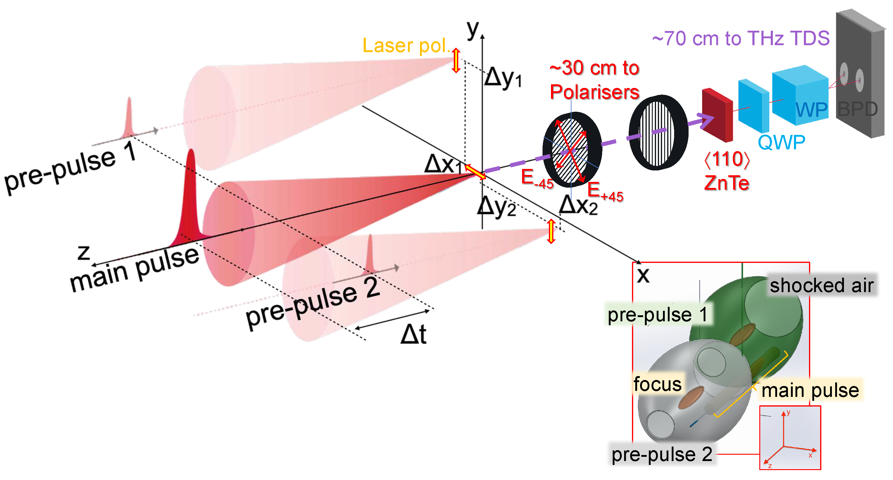
Figure 2.
The THz-TDS waveforms of (a) y-component of the single pre-pulse when the delay time between the pre-pulse and main pulse irradiation is at 9.7 ns. The spatial offset for the pre-pulse irradiation is (, ) = (m, m) for the blue solid line or (m, m) for the red dotted line. (b) The y-component of the dual pre-pulses when (, , ) = (m, m, m) and (, , ) = (m, m, m).
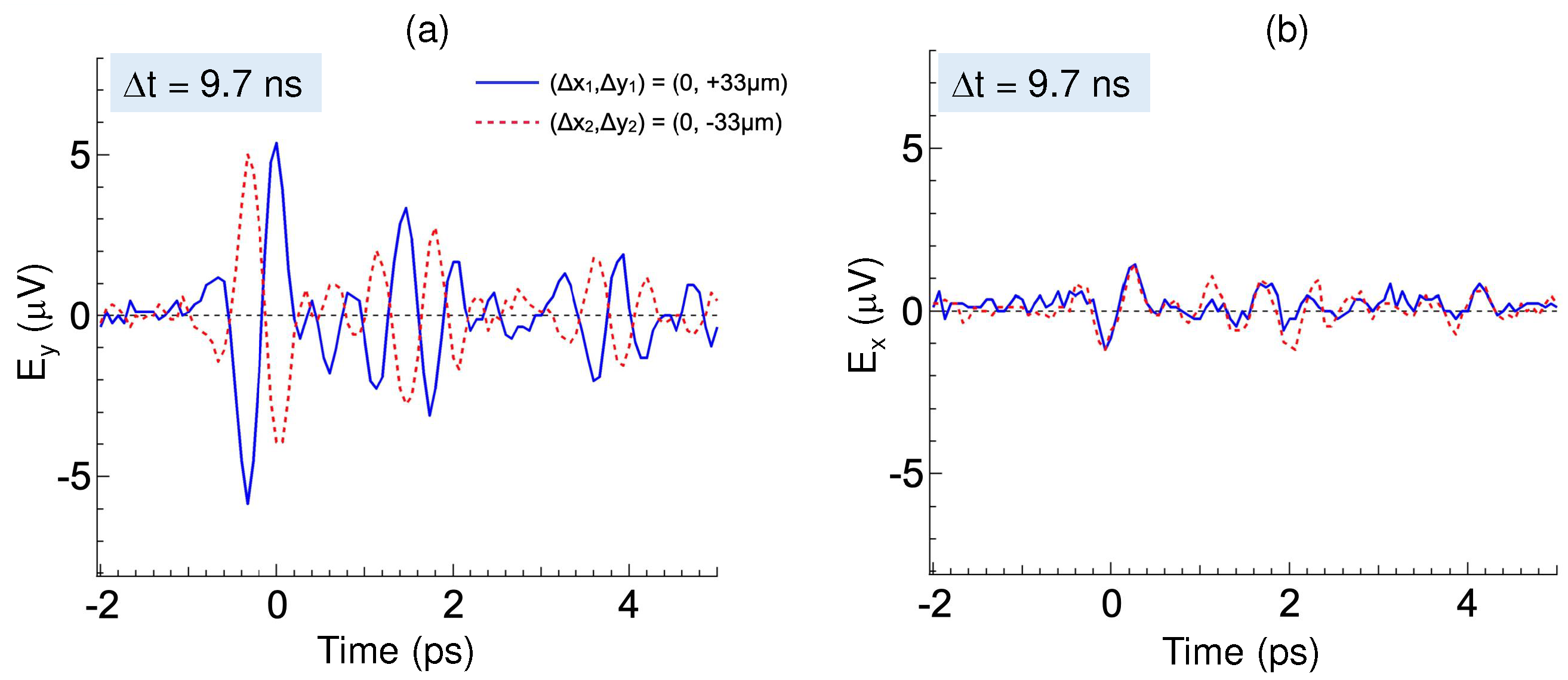
Figure 3.
(a) THz polarization evolution in time shown as a map. (b) Geometry of main pulse (m) and pre-pulses 1,2 (p1,p2). Pre-pulse 1 and the main pulse were fixed, and pre-pulse 2 was scanned along the y-axis. (c) The THz-polarisation intensity as a function of the vertical offset for the second pre-pulse, . is as shown in the inset and is equal to + . The delay time between the pre-pulse and main pulse irradiation is 9.7 ns. The spatial offset for the first pre-pulse irradiation is fixed at (, ) = (m, m) while the position of the second pre-pulse irradiation, and was varied from 0 to m. The blue THz-pol. plot indicates the results from two pre-pulse irradiation with both pre-pulses at 0.2 mJ. The black THz-pol. plot indicates the results from two pre-pulse irradiation with the pre-pulses at 0.2 mJ and the second pre-pulse at 0.05 mJ. The red THz-pol. plot indicates single pre-pulse irradiation condition with the pre-pulse at 0.2 mJ and (, ) = (m, m). The main pulse energy is 0.4 mJ. The red dotted line indicates the THz emission from a single main pulse irradiation in air.
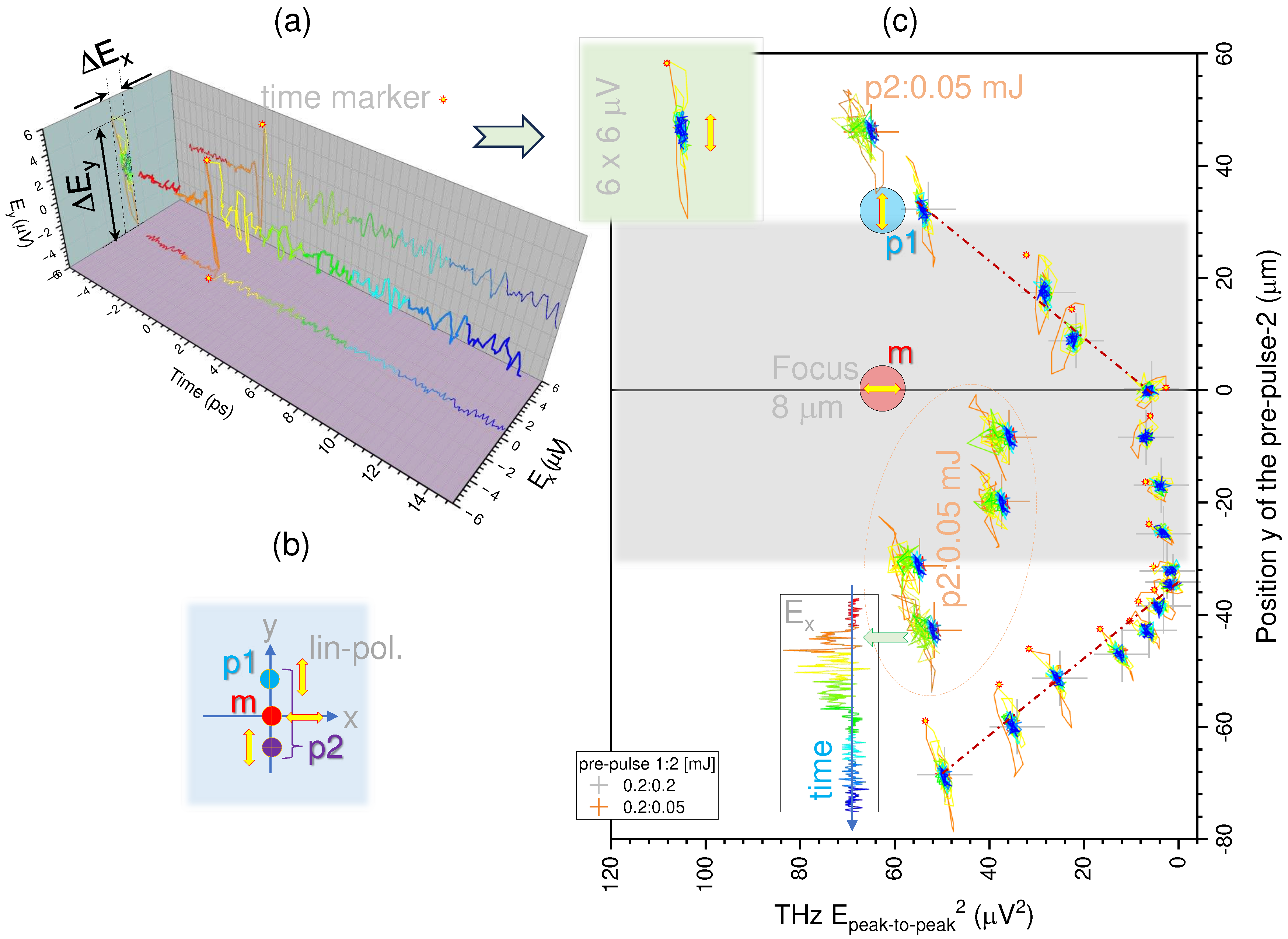
Figure 4.
The THz-polarisation [V2] intensity as a function of the horizontal offset for the second pre-pulse, . The delay time between the pre-pulse and the main pulse is 9.7 ns. The spatial offset for the first pre-pulse irradiation is (, ) = (m, m), while the second pre-pulse is focused at different position with = m (see top-right inset for geometry schematics). The RGB projections () of THz plots are from two pre-pulse irradiation with both pre-pulses at 0.2 mJ. The red THz-pol. plot indicates single pre-pulse irradiation condition with the pre-pulse at 0.2 mJ and (, ) = (m, m). The main pulse energy is 0.4 mJ. The red dotted line indicates the THz emission from single main pulse irradiation in air at V2. The boxed-area (yellow) is V for the -projection maps located at the cross-markers, at which the total intensity is plotted after power calibration. The 3D projection insets illustrate RGB time evolution over a span -5 ps to 15 ps and reveal the sense of polarisation rotation (looking into the beam or time axis); it is plotted for the closest projection RGB markers, respectively.
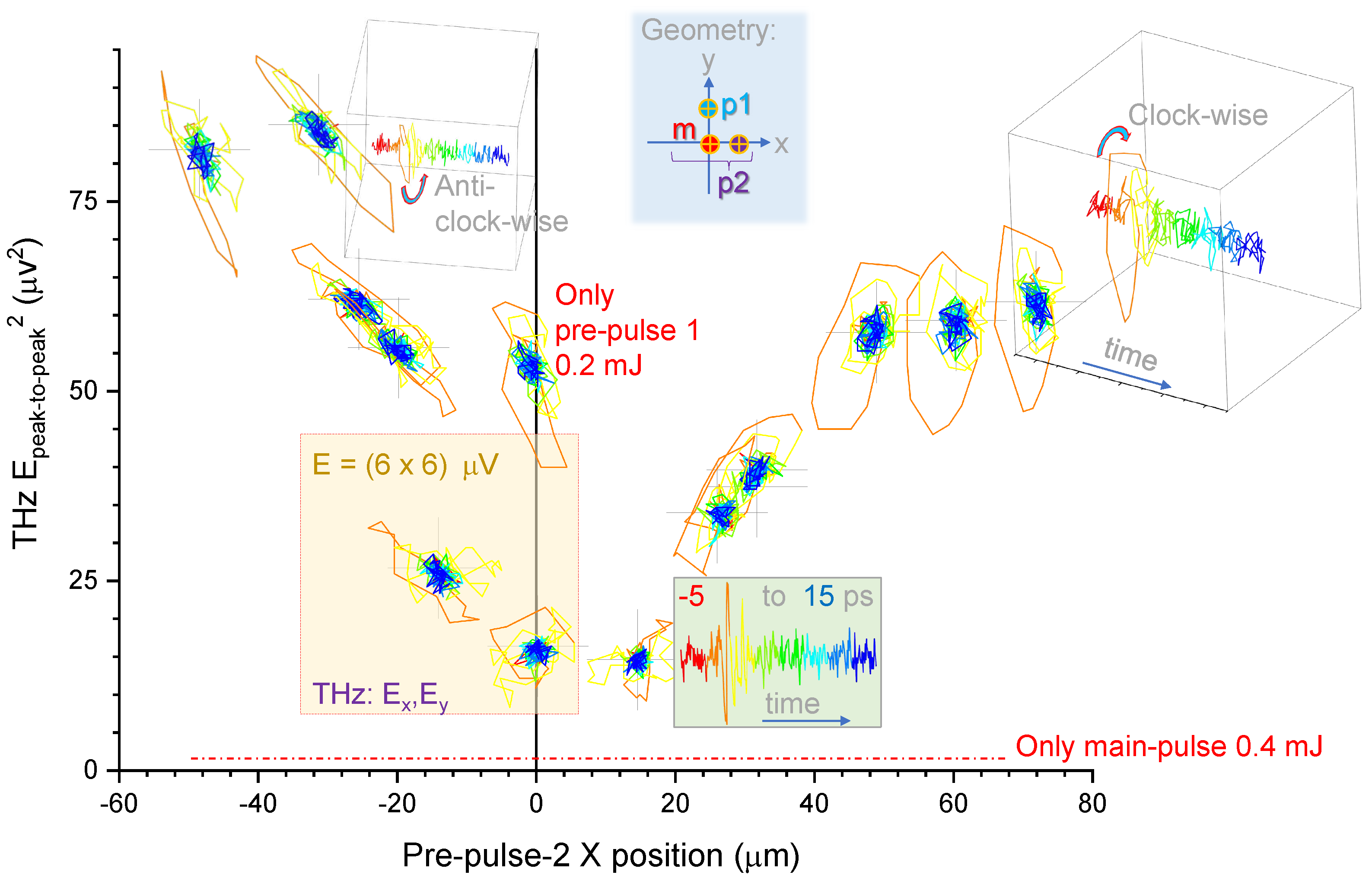
Figure 5.
Ionisation probability (red) and the electron kinetic energy for the parameters of the main pulse interacting with the nitrogen ion and liberation an electron from the level (left) and 5 (right). Pulse duration is 35 fs at FWHM.
Figure 5.
Ionisation probability (red) and the electron kinetic energy for the parameters of the main pulse interacting with the nitrogen ion and liberation an electron from the level (left) and 5 (right). Pulse duration is 35 fs at FWHM.
Figure 6.
Two-pulse enhancement of THz generation in air by the spontaneous magnetic field due to coupled non-parallel gradients of and .
Figure 6.
Two-pulse enhancement of THz generation in air by the spontaneous magnetic field due to coupled non-parallel gradients of and .
Figure 7.
(a) Time and radial dependence of the dimensionless function obtained from a numerical solution of Eq. (9). (b) Distribution of the magnetic field in the plane obtained from the solution of Eq. (8) at time . Arrows show the direction of the electric current. The origin and corresponds to the laser beam axis and the maximum of the plasma density gradient.
Disclaimer/Publisher’s Note: The statements, opinions and data contained in all publications are solely those of the individual author(s) and contributor(s) and not of MDPI and/or the editor(s). MDPI and/or the editor(s) disclaim responsibility for any injury to people or property resulting from any ideas, methods, instructions or products referred to in the content. |
© 2023 by the authors. Licensee MDPI, Basel, Switzerland. This article is an open access article distributed under the terms and conditions of the Creative Commons Attribution (CC BY) license (http://creativecommons.org/licenses/by/4.0/).
Copyright: This open access article is published under a Creative Commons CC BY 4.0 license, which permit the free download, distribution, and reuse, provided that the author and preprint are cited in any reuse.


