
Submitted:
27 November 2023
Posted:
29 November 2023
You are already at the latest version
Abstract
Crop digital twin is redefining traditional farming practices, offering unprecedented opportunities for real-time monitoring, predictive and simulation analysis, and optimization. This research embarks on an exploration of the synergy between precision agriculture, crop modeling, and regression algorithms to create a digital twin for augmenting farmers the concentration and composition prediction-based crop nutrient recovery. This captures the holistic representation of crop characteristics, considering the intricate relationships between environmental factors, nutrient concentrations, and crop compositions. However, the complexity arising from diverse soil and environmental conditions makes nutrient content analysis expensive and time-consuming. This paper presents the result of a predictive digital twin case study that employs six regression algorithms namely Elastic Net, Polynomial, Stepwise, Ridge, Lasso, and Linear Regression to predict rice nutrient content efficiently, particularly considering the coexistence and composition of multiple nutrients. Our research findings highlight the superiority of the Polynomial Regression model in predicting nutrient content, with a specific focus on accurate nitrogen percentage prediction. This insight can be used for nutrient recovery intervention by knowing the precise amount of nutrient to be added into the crop medium. The adoption of the Polynomial Regression model offers a valuable tool for nutrient management practices in the crop digital twin, potentially resulting in higher-quality rice production and a reduced environmental impact. The proposed method can be replicable in other low-resourced crop digital twin system.
Keywords:
rice nutrient level
; fertilizer optimization
; nutrient analysis
; polynomial regression
; nutrient prediction
; environmental impact reduction
1. Introduction
Digital twin technology involves the creation of a virtual duplicate of a physical object or system, enabling the simulation and analysis of diverse scenarios and outcomes [1]. When applied to crop management, a digital twin becomes a powerful tool for modeling a specific farm, considering variables such as soil quality, weather conditions, irrigation systems, and crop varieties. This collected data is then utilized to update the digital twin, facilitating predictions about upcoming crop yields, potential pest outbreaks, and other influential factors that may impact the farm's overall success.
Employing Digital Twins as a primary method for farm management facilitates the separation of physical processes from their planning and control. Consequently, farmers gain the capability to oversee operations and crop health remotely, relying on (almost) real-time digital information rather than depending solely on direct observation and on-site manual tasks [2,3]. The deficiency of vital nutrients can lead to reduced crop yields [4,5]. This empowerment enables prompt action in response to anticipated or unexpected deviations such as crop nutrient concentration and allows for the simulation of the effects of interventions such as nutrient recovery based on real-life data.
In this context, the application of machine learning (ML) offers a promising avenue for farmers. ML equips them with tools for monitoring soil quality and delivering personalized recommendations, drawing insights from both experimental and field data. Nonetheless, the prediction of rice essential nutrients remains a formidable challenge, primarily due to several factors: 1) the inherent variability in nutrient content, 2) the diversity of analytical approaches, 3) limitations in data availability, 4) genetic diversity among rice varieties, and 5) the associated cost and time constraints [7,8,9]. Consequently, it is imperative to address these multifaceted challenges to develop accurate and reliable nutrient prediction models for rice [6,7,8].
This paper report one of our low-resourced digital twin case studies on rice nutrient recovery. Regression, a supervised machine learning technique, holds promise in mitigating these challenges as the method is simple and does not require huge computational processing. This matches the data that we have collected, on the nutrient concentration of the plant across its growth period. Regression facilitates the identification of intricate relationships among essential rice nutrients, ensuring their optimal supply, thereby enhancing rice growth and nutrient content [1,2,3,4,5,6]. Among the myriad regression algorithms, Elastic Net regression, Polynomial regression, Stepwise regression, Ridge regression, Lasso regression, and Linear regression hold particular relevance for predicting nutrient concentration by considering the coexistence and composition of multiple nutrients. These algorithms offer a structured, data-driven approach to unravel the complexities of rice nutrition, providing accurate predictions and contributing to the standardization of nutrient management practices. Moreover, they play a crucial role in fostering sustainable and environmentally friendly rice cultivation practices. The selection of the most suitable regression algorithm depends on the specific characteristics of the dataset, sometimes necessitating the combination of these algorithms to achieve optimal performance.
Given the potential impact of linear and polynomial regression techniques on fertilizer optimization, essential nutrient supply, and ultimately rice quality, this study seeks to identify the most effective regression algorithm for predicting nutrient concentration percentages based on the co-existence and composition of other nutrients. The incorporation of regression algorithms in the crop digital twin is mainly because of its efficiency and effectiveness. This endeavor promises optimized nutrient management practices, culminating in enhanced rice quality and a reduced environmental footprint through the adjustment of nutrient ratios.
This paper unfolds in six sections. The first section underscores the significance of predicting rice essential nutrients and elucidates the challenges in this domain, along with the role of linear and polynomial regression algorithms in addressing these issues. The second section offers an overview of the dataset and its attributes. The third section delineates the flowchart of the polynomial regression algorithm. The fourth section introduces the evaluation metrics employed to assess algorithm performance. The fifth section presents the experimental results and their comprehensive analysis. Finally, the paper concludes by summarizing the findings and proposing potential avenues for future research.
2. Literature Review
One of the promises of digital twin in crop management is for automatic prediction system to support deciding the appropriate fertilization period [1]. Deploying the sensors which monitors concentration of nutrients present in soil, humidity, and temperature in the real fields to make the consistent quality check. Machine learning could be used as a proactive measure as predictor of the degradation of crop medium’s and crop’s plant nutrients which could increase the risk of crop pests and diseases.
Regression algorithms play a central role in rice nutrient prediction by unraveling the intricate interplay of nutrients in rice cultivation. Elastic Net Regression, Polynomial Regression, Stepwise Regression, Ridge Regression, Lasso Regression, and Linear Regression provide essential insights into the complex relationships among soil composition, environmental variables, and agricultural practices. These algorithms empower researchers to comprehend the often-nonlinear dependencies among these factors, deepening our understanding of how various nutrients influence rice nutrition.
Regression algorithms are data-driven, offering a robust framework for analyzing and interpreting nutrient data from diverse sources. By harnessing historical data and observational insights, these algorithms provide crucial guidance on how different nutrients impact rice composition. This knowledge is vital for optimizing fertilizer usage, enhancing nutrient management, and ultimately improving rice quality and yields.
These algorithms also aid farmers, agricultural experts, and policymakers in making informed decisions about crop management, fertilization strategies, and soil enrichment. This proactive approach helps avoid over-fertilization or under-fertilization, mitigating their detrimental effects on crop health and environmental sustainability.
Existing works on rice nutrient has focused on predicting essential nutrient levels in rice, such as N, P, K, Mg, and Ca, and their effects on rice plant growth and development. One study employed an artificial neural network-based prediction algorithm to assess the influence of individual nutrients (N, P, K, Zn, and S) on various rice plant parameters. The algorithm indicated that optimal growth often occurs with nutrient doses below the maximum applied levels, while maximum yield is achieved at 100% nutrient dose [10].
Another study used regression methods and found that random forest regression algorithms provided the highest accuracy for estimating rice shoot dry matter, leaf area index, and nitrogen accumulation [11]. A third study evaluated different approaches for estimating rice aboveground biomass, plant nitrogen uptake, and nitrogen nutrition index, with the random forest algorithm demonstrating superior performance [12]. An additional study focused on using machine learning for early detection of nutrient deficiency in rice through leaf image processing, achieving high testing accuracy and roc_auc score [4].
Rice nutrient content prediction, based on the composition of other nutrient information, including nitrogen, phosphorus, potassium, and organic matter as input variables, was addressed in a study [14]. This study compared the Elastic Net regression algorithm with traditional linear regression methods, including Ordinary Least Squares (OLS) regression, Ridge regression, and Lasso regression. The results highlighted the superior performance of the Elastic Net regression algorithm, exhibiting higher R-squared scores (R2) and lower Mean Absolute Error (MAE). Thus, Elastic Net proves more accurate in predicting rice nutrient content and its correlation with other nutrients.
Essential nutrient levels in rice can also be predicted using spectral data from remote sensing [15], considering nutrients like N, P, K, Mg, and Ca. This research compared the polynomial regression algorithm with two other methods: Multi linear regression (MLR) and Partial least squares regression (PLSR). The outcome demonstrated the polynomial algorithm's superiority in predicting nutrient concentrations in rice levels.
Other studies predicting nutrient content in rice used 16 nutrients as predictors, such as moisture, crude protein, fat, ash, total dietary fiber, soluble dietary fiber, insoluble dietary fiber, total sugar, sucrose, glucose, fructose, amylose, amylopectin, total amino acids, lysine, and thiamine [16]. These studies employed three algorithms: stepwise regression, PLSR, and MLR for prediction. The results favored stepwise regression analysis for its superior accuracy in predicting nutrient content in rice.
Another study aimed to predict nutrient content in rice based on 14 nutrients, including moisture, crude protein, fat, ash, total dietary fiber, soluble dietary fiber, insoluble dietary fiber, total sugar, sucrose, glucose, fructose, amylose, amylopectin, and thiamine. This research compared three algorithms: ridge regression, principal component regression (PCR), and PLSR. Ridge regression stood out as the most effective method for predicting nutrient content in rice, delivering higher accuracy than PLSR and PCR.
Utilizing another set of 14 nutrients, including moisture, crude protein, fat, ash, total dietary fiber, soluble dietary fiber, insoluble dietary fiber, total sugar, sucrose, glucose, fructose, amylose, amylopectin, and thiamine as predictors for nutrient prediction in rice, another study employed three algorithms: MLR, PLSR, and lasso regression. The experimental results highlighted the precision of the lasso regression algorithm in predicting both yield and nutrient content in rice, offering potential benefits in optimizing rice crop cultivation and management.
In a similar vein, another study [19] compared three prediction algorithms, namely MLR, PLSR, and PCR, for nutrient content in rice, considering nutrients such as moisture, crude protein, fat, ash, total dietary fiber, soluble dietary fiber, insoluble dietary fiber, total sugar, sucrose, glucose, fructose, amylose, amylopectin, and thiamine. The findings indicated that MLR provided more accurate predictions compared to the other methods assessed.
Table 1 provides a comparative analysis of the advantages and disadvantages of regression algorithms [14,15,16,17,18] for rice nutrient prediction. These algorithms effectively capture both linear and nonlinear correlations among various nutrients.
These diverse regression algorithms collectively share a common aim: to enhance the precision and reliability of predictions concerning rice nutrient content, a critical step in optimizing fertilizer application, ensuring a balanced nutrient supply, and ultimately elevating rice crop quality and yield while reducing environmental impact.
However, very limited works have addressed the crop’s nutrients prediction by focusing on the co-existent and composition nutrient’s concentration. For a digital twin system equipped with crop nutrients surveillance, this comes to our advantage to enable crop nutrient recovery. Our exploration and application of these regression techniques serve to address prevailing research disparities and foster a more standardized and comprehensive approach to predicting rice nutrient content. By employing a variety of regression models, our objective is to gain a deeper understanding of the intricate relationships among different nutrients in rice. This, in turn, promotes more sustainable and efficient rice cultivation practices.
3. Materials and Methods
This part splits into three subsections. First, we explain the dataset and its attribute. Next, we present the setting of the regression models. Then, we discuss the evaluation metrics.
3.1. Dataset Description
A self-collected rice dataset was used as described in Table 2, comprising of 348 observations and nine attributes. This multivariate dataset features a combination of categorical and numerical data, including spatiotemporal factors such as Season, Day, Plot, and Subplot.
The Season attribute categorizes data into two distinct seasons, denoted by the values 1 and 2, enabling the exploration of how seasonal changes influence rice nutrient levels, a fundamental aspect of rice production optimization. Additionally, the Day attribute, with three distinct values—30, 60, and 90, introduces temporal granularity, facilitating an examination of nutrient content variations within each season. This temporal dimension is essential for understanding the influence of specific days on nutrient levels.
Furthermore, the Plot attribute categorizes data into four distinct plot locations represented by values 1, 3, 4, and 5, enabling the assessment of nutrient distribution across different areas within the study site, thus adding a spatial context to the analysis. Subplot further refines the spatial information by specifying 15 sublocations within each plot, denoted by values such as 1A, 1B, 1C, and so forth.
This fine-grained attribute is invaluable for scrutinizing nutrient variation within specific subregions of the plots, enhancing spatial precision. Additionally, the dataset incorporates nutrient concentration, composition and co-existence ('N%', 'P%', 'K%', 'Mg%', 'Ca%'), which is vital for understanding rice growth and health. The dataset's integrity is maintained, as it contains no missing values.
Figure 1 shows the dashboard that presents the average rice nutrient concentration across the growth period and the rice anatomical values at harvesting time. From this diagram, we could identify the relationship of the nutrient con-existence, composition and concentration with the yield. The digital twin supports three-staged insight for the crop intelligence. First, we could also see the average values of nutrients that has led to the yield, and the nutrient values from the plant with the best yield becomes the benchmark. So, this has motivated us towards the second intelligence by predicting the co-existence, concentration and composition of the plant at each plot and subplot to know their health. The third intelligence is nutrient recovery during the growth as an intervention mechanism so that when the predicted values can be a guide on precise additional nutrient to be added into the crop medium as an effort to optimize the yield. The precision of values for additional nutrient can mitigate for unnecessary excess in fertilizer usage and waste pollution.
3.3. Data Pre-Processing Using Min-Max Normalization
The Min-Max normalization method is applied to rescale the input features between 0 and 1 during the pre-processing phase. This normalization technique is suitable for the prediction models of this study because it helps to ensure that all the input features are on the same scale and have the same range, which helps the linear regression models of this study converge faster and boost their performance. This approach removes noises from data and prevents the big scales from data by giving the range of [0,1]. Equation (1) shows the formula of the Min-MAX method.
Where X is the original value of a data point, is the minimum value in the dataset, is the maximum value in the dataset, andis the normalized value of the data point. This formula ensures that the minimum value in the dataset is scaled to 0 and the maximum value is scaled to 1, with all other values falling between these two limits.
By applying a preprocessing method to the dataset, we can improve the stability and performance of regression models. Once this stage is complete, we can proceed to the next stage, where we design a regression model based on the different variables in the dataset. This stage involves selecting an appropriate regression method and specifying the independent and dependent variables. Finally, we analyze the model and provide information on its performance and accuracy. Figure 2 illustrates the Rice Nutrients data before and after applying the Min-Max normalization method. The visual representation of the data highlights the impact of normalization on the distribution of nutrient concentrations.
The dataset under analysis consists of nutrient concentration data for rice samples, including attributes like nitrogen (N %), phosphorus (P %), potassium (K %), magnesium (Mg %), and calcium (Ca %). Prior to visualization, the data exhibited variations in nutrient concentrations that prompted the need for exploration. The raw data contained outliers, which are data points significantly different from the majority of the observations. These outliers, if not addressed, can impact the understanding of the overall nutrient distribution and make it challenging to discern patterns and trends in the data.
Therefore, to gain a deeper understanding of the nutrient concentration data and visualize its distribution, we employed box plots both before and after applying Min-Max normalization. The original box plots revealed the presence of outliers in the dataset, which was affecting the clarity of the distribution. To address this issue, Min-Max normalization was applied to scale the data. The box plots after normalization effectively showcased the distribution of nutrient concentrations without displaying outliers. This approach allows for a more accurate and informative representation of the data, aiding in the identification of central tendencies and variations while providing a clearer view of the data's overall structure. The use of box plots before and after normalization aids in the assessment of data quality and the impact of data preprocessing techniques.
3.3.1. Prediction Models Design Based on Various Features
Various models have been implemented based on different features of rice dataset as shown in Table 3 based on exploiting the nutrient concentration, co-existence and composition. In Table 3, ‘Y’ indicates that the features {spatiotemporal factors, nutrients} are used in the model building, while ‘N’ indicates otherwise. All six regression algorithms are applied to develop the models.
3.4. Flow Chart Polynomial Regression Model
Six linear regression models (designated as Models 1 to 6, as shown in Table 3) were employed to predict essential nutrient levels in rice using the dataset. The design and evaluation of the polynomial regression model, which outperformed other linear regression models, are outlined in Figure 3. Model evaluation results are presented in Section 5.
The flowchart in Figure 3 outlines the steps for predicting rice nutrient content using a polynomial regression model, as a representation of the six designed models in this study. These steps are explained below:
Collect the rice dataset
- Preprocess the data using the Min-Max normalization method to improve model stability and performance
- Select a set of variables as predictors to create a designed regression model
- Choose the degree of the polynomial regression model (degree=2) to balance model complexity and fit flexibility
- Create a polynomial regression model using the 80% of whole data as the training data.
- Fit the polynomial regression model to the training data to optimize the model parameters
- Evaluate the model's performance using testing data and three metrics: Mean Absolute Error (MAE), R-squared value, and Root Mean Squared Error (RMSE)
- Use the trained model to predict nutrient content for new rice samples based on their predictor variables
- Evaluate the predicted nutrient values against actual nutrient values
- Iterate and improve the model as necessary based on evaluation results.
3.5. Regression Models using Nutrients Concentration, Co-existence and Composition
This section provides a mathematical overview of the polynomial regression model and showcases its superior performance over other linear regression methods. Polynomial regression is a type of multivariate regression analysis that models the relationship between dependent and independent variables of this research using an nth degree polynomial, as expressed in Equation (2).
where, is the dependent variable, is the independent variable, , , , ..., are the regression coefficients or parameters, and ɛ is the error term or residual. The degree of the polynomial regression model is determined by the value of n.
The dependent variable of this investigation, is divided into two categories of single and multi-dependent variables where the {N%},{P%},{K%}, {CA%}, and {Mg%}, and {N% ,P%, K%, CA%, and Mg%} are belong to single and multi-dependent variables respectively. This investigation considers two categories of dependent variables: single-dependent variables, such as N%, P%, K%, Ca%, and Mg%; and multi-dependent variables, which consist of combinations of N%, P%, K%, Ca%, and Mg%.
The pseudocode for the nutrient prediction based on other nutrients co-existence, concentration and composition using the Polynomial Regression is provided as follows:
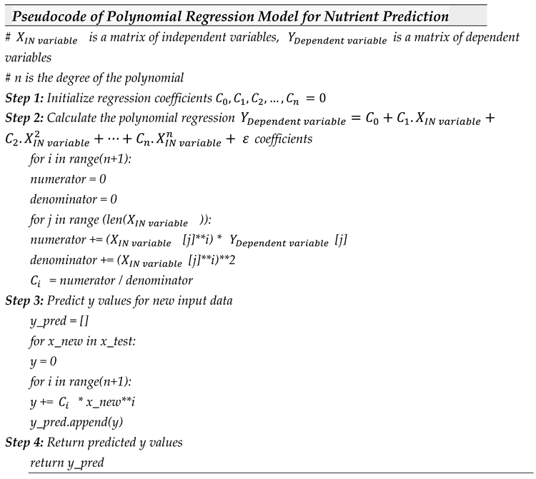
The polynomial regression algorithm in the provided pseudocode is built using four steps. In Step 1, the regression coefficients are initialized. In Step 2, Equation (2) is used to calculate the polynomial regression coefficients by iterating over the data points in the input matrices (representing the independent variable) and (representing the dependent variable). In Step 3, the algorithm uses the polynomial function (refer to Equation (2)) to predict nutrient levels for new input data. Finally, the algorithm outputs the predicted nutrient levels.
The polynomial method tackles the issue of other linear regression techniques by capturing non-linear relationships between the independent and dependent variables. Therefore, this scheme other regression models, including Elastic Net Regression, Stepwise Regression, Ridge Regression, Lasso Regression, and Simple Linear Regression, when the relationship between the independent and dependent variables is non-linear.
3.6. Evaluation Metrics
Three metrics of 1) R-squared, 2) MAE, and 3) RMSE have been used for evaluating the performance of linear regression techniques. The explanations of these metrics are presented below:
- 1.
- R-Squared: It considered as a statistical measure that represents the proportion of the variance in the dependent variable that is explained by the independent variables in the model. It ranges from 0 to 1, with a higher value indicating a better fit of the model to the data. The R-squared formula is stated in Equation (3).where is the sum of squares of residuals and is the total sum of squares.
- 2.
- Mean Absolute Error (MAE): MAE measures the average absolute difference between the predicted values and the actual values. It is a measure of how close the predictions are to the actual values, on average.
- 3.
- Root Mean Squared Error (RMSE): RMSE measures the square root of the average squared difference between the predicted values and the actual values. It is a measure of how well the model is able to predict the actual values.where n is the number of observations, is the predicted value and is the actual value.
4. Experimental Setting
In the initial step of this research, six common linear regression methods were used to predict essential nutrients in rice. The main purpose is to identify the best prediction method that could support the precision of nutrient recovery. This is because, if we could predict the nutrient concentration during growth, intervention mechanism such as adding fertiliser to match the benchmark plant could be performed. Nutrient co-existence, concentration and composition (Table 3) are used to develop and investigate the performance of the regression methods include Elastic Net Regression, Polynomial Regression, Stepwise Regression, Ridge Regression, Lasso Regression, and Linear Regression.
The data was then split into training and testing sets using the train_test_split() function from the sklearn.model_selection module. The size of the training and testing data was set to 80% and 20%, respectively. The random_state was also set to 42 to ensure that the split was reproducible. For each of the models, the fit() method was called on the training data (X_train and y_train), and the predict() method was then called on the testing data (X_test) to generate the predicted values (y_pred). The evaluation metrics (R2 score, RMSE, and MAE) were then calculated using the predicted values (y_pred) and the actual values (y_test). This process was repeated for each of the six models.
5. Results and Discussion
This section presents the experimental results for Elastic Net Regression, Polynomial Regression, Stepwise Regression, Ridge Regression, Lasso Regression, and Linear Regression to predict rice nutrient levels using Model 1 until 6. Table 4 and Figure 4 displays the RMSE score of all six models where polynomial regression has the best performance in four models to predict Ca%, K%, P% and N% with an average of 0.1502 RMSE, except Model 2 (prediction of Mg%), with very little standard deviation (0.1980).
The best performance of algorithm for Model 2 is Linear Regression. In terms of the performance to predict each nutrient, Model 2 is the easiest to be predicted, based on the average (AVG) of RMSE for this model, at 0.0219 (Figure 5). On the contrary, according to Figure 6, the percentage of N is the most difficult and inconsistent performance across the regression models, with an average of RMSE at 0.5638.
The detailed performance results using R2, MAE and RMSE for the six designed models developed using each regression model are provided in Table 5, Table 6, Table 7, Table 8, Table 9 and Table 10, respectively.
Based on the conducted experiments for Model 1, the polynomial regression method produces better performance in comparison to the other tested models in terms of higher R-square scores and lower values of MAE and RMSE. Thus, this scheme is considered the best method for the prediction of nutrient content for Model 1.
Based on the experiments conducted for Model 2, it can be concluded that the linear regression method is the most suitable approach for rice nutrient prediction. This method outperformed the other tested models with higher R-square score and lower values of MAE and RMSE, indicating better predictive performance.
Also, Table 7 showed that the polynomial regression method is the most appropriate approach for rice nutrient prediction for Model 3. Because this technique generates a higher R-square score and lower value of MAE and RMSE compared to other methods.
Likewise, the best technique for nutrient rice prediction using Model 4 is the polynomial regression method. This is due to a higher R-square score and lower value for RMSE and MAE. Therefore, this approach can offer more precise predictions in comparison to the other tested techniques.
Similarly, the polynomial regression technique has the highest R-Square score with a lower value for MAE and RMSE in comparison to the other models for Model 5. Hence, this scheme can yield more accurate predictions for rice nutrients.
Finally, for the last model also the polynomial regression method produced the highest R-Square score with a lower value for MAE and RMSE in comparison to the other models for Model5. Consequently, this scheme can yield more accurate predictions for rice nutrients.
The experiments results led us to the conclusion that regression models have good performance to inform nutrients co-existence, concentration and composition. This insight allows intervention to increase the nutrient recovery to optimise the crop’s yield. The polynomial regression model generally outperformed the other tested algorithms in terms of producing higher R-square values, and lower MAE and RMSE values for almost all models. This is due to the ability of the polynomial function to capture nonlinear relationships among variables. However, it should be noted that for Model 2, the polynomial regression algorithm produced a negative R-square value, indicating that it explained less variance in the dependent variable than a horizontal line. Therefore, the polynomial function was not well-suited for predicting nutrient content in Model 2. In contrast, the linear regression algorithm produced better performance compared to the other methods for Model 2, signifying that this model was better approximated by a straight-line relationship. This finding highlights the significance of considering the specific nature of the data and the relationships between variables when selecting the most appropriate regression model for nutrient prediction.
5.1. Statistical Analysis
For this investigation, we chose to use parametric statistical analysis because the assumptions of normality and equal variance are likely to be met given the data and the fact that we are comparing means within each regression model. Additionally, parametric tests are generally more powerful than non-parametric tests, meaning they have a greater ability to detect differences between groups when they exist.
The ANOVA is used to test for differences between the six regression models because we are comparing more than two groups. ANOVA is a powerful test that can detect differences between multiple groups while controlling for Type I error rate. By using ANOVA, we can test whether there is a significant difference between the six regression models as a whole, rather than testing each model against every other model individually. This approach can help us identify which models are generally more effective than others in predicting the outcome variable. Table 11 present the ANOVA test for six designed regression model using different regression methods of “Elastic Net Regression”, “Polynomial regression”, “Stepwise regression”, “Ridge regression”, “Lasso regression”, and “Linear Regression”.
Based on the ANOVA test with a p-value of 2.3253E-17 and an alpha level of 0.05, we can conclude that there is a statistically significant difference among the six designed regression models. Therefore, we reject the null hypothesis that there is no significant difference and accept the alternative hypothesis that at least one of the regression models has a different performance value than the others.
Based on the results of the ANOVA test, Model 5 demonstrated better performance compared to other designed feature set models (Refer to Table 3). As a result, to gain insight into the impact of each nutrient on N% nutrient concentration, we utilized SHAP visualization. Figure 7 illustrates the effect of each nutrient on N% nutrient concentration.
Referring to Figure 7, the attributes K (Potassium), Mg (Magnesium), Day, Season, Ca (Calcium), Plot, SubPlot, and P (Phosphorus) appear to have varying levels of impact on N% nutrient concentration. Potassium (K) has the highest impact, followed by Magnesium (Mg), indicating that their concentrations in the soil or nutrient supply significantly influence N%. The day and season when measurements are taken also play essential roles, while attributes like Calcium (Ca), Plot, SubPlot, and Phosphorus (P) have varying degrees of influence, with P showing the lowest impact. Therefore, this visualization can be valuable for optimizing agricultural and environmental practices to manage nutrient levels effectively, considering specific local conditions and domain knowledge.
6. Conclusion and Future Work
Crop digital twin offers a revolution to monitor and intervene crop health management. The physical twin surveil the condition of the crop and this information can be analysed by the digital twin to provide suggestions for countermeasures such as adding nutrient concentration level.
Predicting nutrient levels is crucial for optimizing fertilizer usage and ensuring a balanced nutrient supply, leading to higher-quality and increased yields, and reduced environmental impact. The importance of accurately anticipating essential nutrients, such as Nitrogen (N), Phosphorus (P), Potassium (K), Calcium (Ca), and Magnesium (Mg), in rice cannot be overstated, as it directly impacts crop yield, quality, and environmental sustainability. The challenges in this field stem from the complexities introduced by the variability in nutrient content, the diversity of analytical approaches, data availability constraints, genetic diversity, and the associated costs and time investments.
To address these challenges, this research has explored a range of regression algorithms, including Elastic Net Regression, Polynomial Regression, Stepwise Regression, Ridge Regression, Lasso Regression, and Linear Regression, to predict rice nutrient content. These algorithms have proven to be invaluable tools for capturing both linear and nonlinear correlations among various nutrients, offering a structured, data-driven approach to understanding and managing the complexities of rice nutrition.
The findings reveal that the Polynomial Regression algorithm consistently outperforms the other models for predicting several nutrients, particularly Calcium (Ca%), Potassium (K%), Phosphorus (P%), and Nitrogen (N%). This algorithm's ability to handle both small and large datasets, along with its proficiency in capturing nonlinear relationships, makes it a favorable choice for optimizing nutrient management practices. It is important to note, however, that Model 2, focused on predicting Magnesium (Mg%), demonstrated a unique characteristic, as Linear Regression outperformed Polynomial Regression.
The dashboard in the digital twin visualizes the current nutrient content of the crop as a surveillance mechanism while the predicted nutrient concentration is a valuable insight for precise fertilisation to be added as nutrient recovery. This may mitigate fertilisation overload and waste pollution. Albeit manual intervention is currently addressed in this research, the regression method’s implementation supports low-resourced crop digital twin so that fast computation could be performed.
In summary, these regression models provide essential insights into rice nutrient prediction, offering a pathway to optimize fertilizer use, ensure balanced nutrient supply, enhance rice quality, and reduce environmental impact. They contribute to the development of standardized methodologies for nutrient prediction and promote more sustainable and environmentally friendly rice cultivation practices. The choice of the most suitable regression model depends on the specific characteristics of the dataset and the nature of the nutrient interactions. Therefore, the selection of the appropriate algorithm is pivotal to achieving the highest predictive accuracy for rice nutrient content.
Acknowledgments
This paper reports some progress in our project entitled Digital Twin Prototype for Integrated Multi-Enterprise Agricultural Monitoring Mechanism, funded by the Universiti Putra Malaysia, Malaysia.
References
- C. Verdouw, B. C. Verdouw, B. Tekinerdogan, A. Beulens, and S. Wolfert, “Digital twins in smart farming,” Agric. Syst., vol. 189, no. January, p. 103046, 2021. [CrossRef]
- S. De Alwis, Z. Hou, Y. Zhang, M. H. Na, B. Ofoghi, and A. Sajjanhar, “A survey on smart farming data, applications and techniques,” Comput. Ind., vol. 138, p. 103624, 2022. [CrossRef]
- C. Prakash, L. P. C. Prakash, L. P. Singh, A. Gupta, and S. K. Lohan, “Advancements in smart farming: A comprehensive review of IoT, wireless communication, sensors, and hardware for agricultural automation,” Sensors Actuators A Phys., vol. 362, no. August, p. 114605, 2023. [CrossRef]
- Cho, J.; Lee, J. Multiple Linear Regression Models for Predicting Nonpoint-Source Pollutant Discharge from a Highland Agricultural Region. Water 2018, 10, 1156. [Google Scholar] [CrossRef]
- Zaukuu, J.-L.Z.; Benes, E.; Bázár, G.; Kovács, Z.; Fodor, M. Agricultural Potentials of Molecular Spectroscopy and Advances for Food Authentication: An Overview. Processes 2022, 10, 214. [Google Scholar] [CrossRef]
- Ali, Y.; Raza, A.; Iqbal, S.; Khan, A.A.; Aatif, H.M.; Hassan, Z.; Hanif, Ch.M.S.; Ali, H.M.; Mosa, W.F.A.; Mubeen, I.; et al. Stepwise Regression Models-Based Prediction for Leaf Rust Severity and Yield Loss in Wheat. Sustainability 2022, 14, 13893. [Google Scholar] [CrossRef]
- Tangendjaja, B. Nutrient Content Of Soybean Meal From Different Origins based on Near Infrared Reflectance Spectroscopy. Indones. J. Agric. Sci. 2020, 21, 39. [Google Scholar] [CrossRef]
- Cule, E.; De Iorio, M. Ridge Regression in Prediction Problems: Automatic Choice of the Ridge Parameter. Genetic Epidemiology 2013, 37, 704–714. [Google Scholar] [CrossRef] [PubMed]
- Andriopoulos, V.; Kornaros, M. LASSO Regression with Multiple Imputations for the Selection of Key Variables Affecting the Fatty Acid Profile of Nannochloropsis Oculata. Marine Drugs 2023, 21, 483. [Google Scholar] [CrossRef] [PubMed]
- Hayat, A.; Amin, M.; Afzal, S.; Muse, A.H.; Egeh, O.M.; Hayat, H.S. Application of Regression Analysis to Identify the Soil and Other Factors Affecting the Wheat Yield. Advances in Materials Science and Engineering 2022, 2022, 1–10. [Google Scholar] [CrossRef]
- De Borja Reis, A.F.; Moro Rosso, L.; Purcell, L.C.; Naeve, S.; Casteel, S.N.; Kovács, P.; Archontoulis, S.; Davidson, D.; Ciampitti, I.A. Environmental Factors Associated With Nitrogen Fixation Prediction in Soybean. Front. Plant Sci. 2021, 12, 675410. [Google Scholar] [CrossRef] [PubMed]
- Lee, Y.; Choi, Y.; Ahn, D.; Ahn, J. Prediction Models Based on Regression and Artificial Neural Network for Moduli of Layers Constituted by Open-Graded Aggregates. Materials 2021, 14, 1199. [Google Scholar] [CrossRef] [PubMed]
- Lusiana, E.D.; Musa, M.; Ramadhan, S. The Estimation of Nutrient Limit for Predicting Eutrophication Using Quantile Regression Model (Case Study: Aquaculture Pond at IBAT Punten, Batu). IOP Conf. Ser.: Earth Environ. Sci. 2019, 239, 012002. [Google Scholar] [CrossRef]
- Williamson, J. Improving Risk Prediction for Depression via Elastic Net Regression - Results from Korea National Health Insurance Services Data.
- Yanova, M.A.; Oleynikova, E.N.; Khizhnyak, S.V. Polynomial Regression as a Tool for Prediction Quality of Bread Baked of Wheat Flour Mixed with Flour of Cereal Extrudates. IOP Conf. Ser.: Earth Environ. Sci. 2019, 315, 032026. [Google Scholar] [CrossRef]
- Jamshidi, S.; Yadollahi, A.; Ahmadi, H.; Arab, M.M.; Eftekhari, M. Predicting In Vitro Culture Medium Macro-Nutrients Composition for Pear Rootstocks Using Regression Analysis and Neural Network Models. Front. Plant Sci. 2016, 7. [Google Scholar] [CrossRef]
- Ahmed, A.A.M.; Sharma, E.; Jui, S.J.J.; Deo, R.C.; Nguyen-Huy, T.; Ali, M. Kernel Ridge Regression Hybrid Method for Wheat Yield Prediction with Satellite-Derived Predictors. Remote Sensing 2022, 14, 1136. [Google Scholar] [CrossRef]
- Osco, L.P.; Ramos, A.P.M.; Faita Pinheiro, M.M.; Moriya, É.A.S.; Imai, N.N.; Estrabis, N.; Ianczyk, F.; Araújo, F.F.D.; Liesenberg, V.; Jorge, L.A.D.C.; et al. A Machine Learning Framework to Predict Nutrient Content in Valencia-Orange Leaf Hyperspectral Measurements. Remote Sensing 2020, 12, 906. [Google Scholar] [CrossRef]
- Kang, Y.; Nam, J.; Kim, Y.; Lee, S.; Seong, D.; Jang, S.; Ryu, C. Assessment of Regression Models for Predicting Rice Yield and Protein Content Using Unmanned Aerial Vehicle- Based Multispectral Imagery. Remote Sensing 2021, 13, 1508. [Google Scholar] [CrossRef]
Figure 1.
Dashboard about the average nutrient values and the content in the rice.
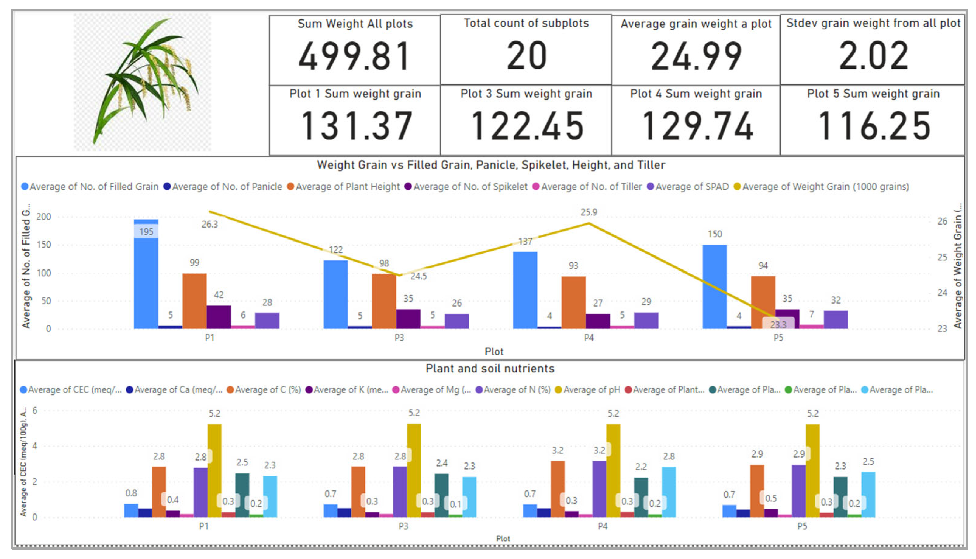
Figure 2.
Rice Nutrient Data: (a) Original Data and (b) Min-Max Normalized Data.
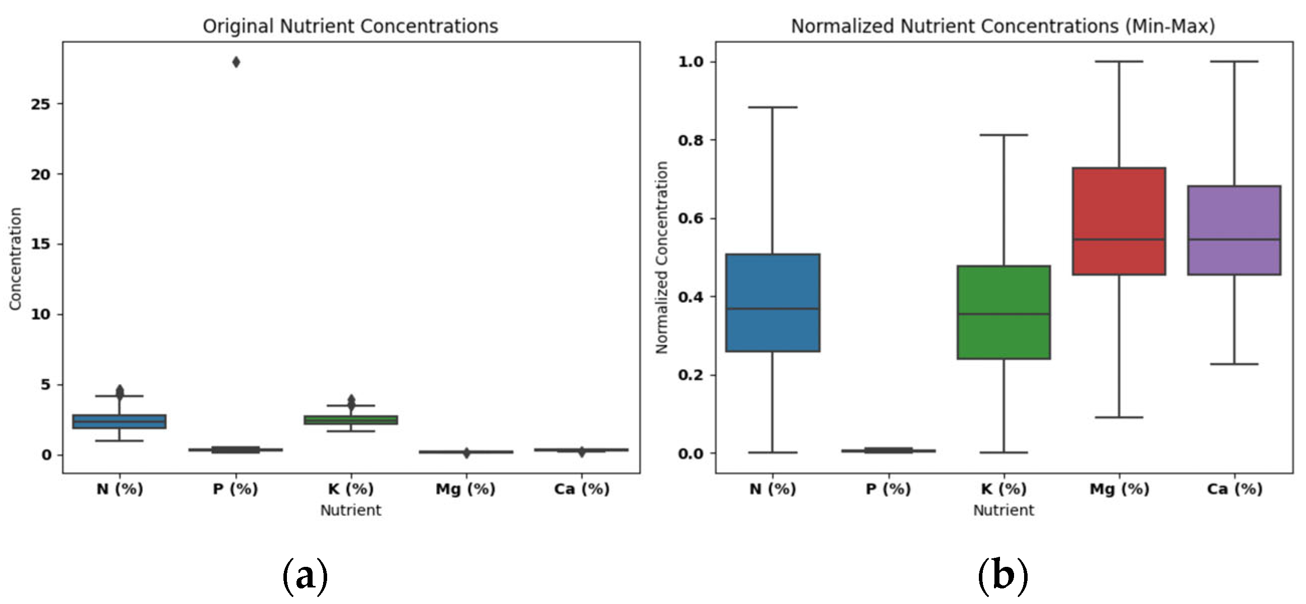
Figure 3.
Flowchart of polynomial regression model for rice nutrients prediction.
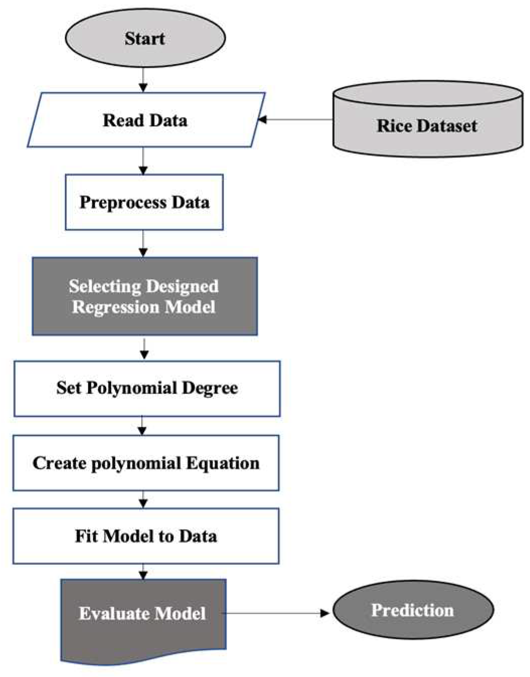
Figure 4.
RMSE performance for each nutrient prediction models.

Figure 5.
Average and stdev score of the regression algorithms.
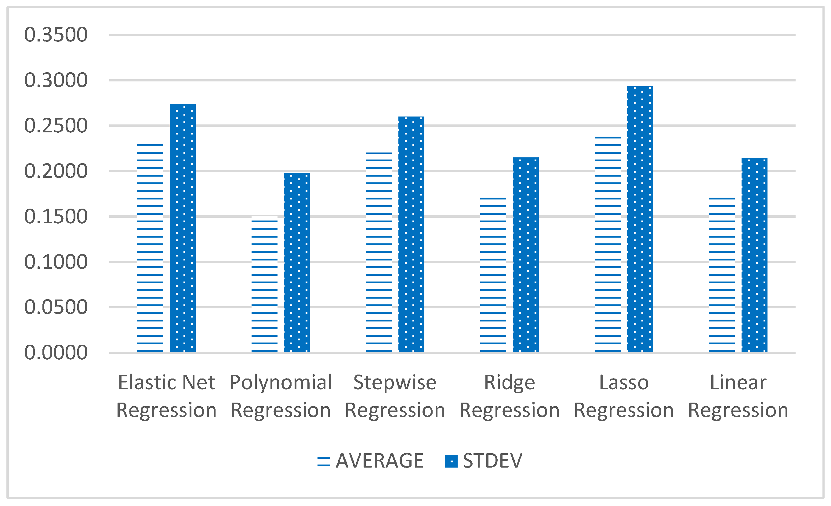
Figure 6.
Average and stdev score of each model.
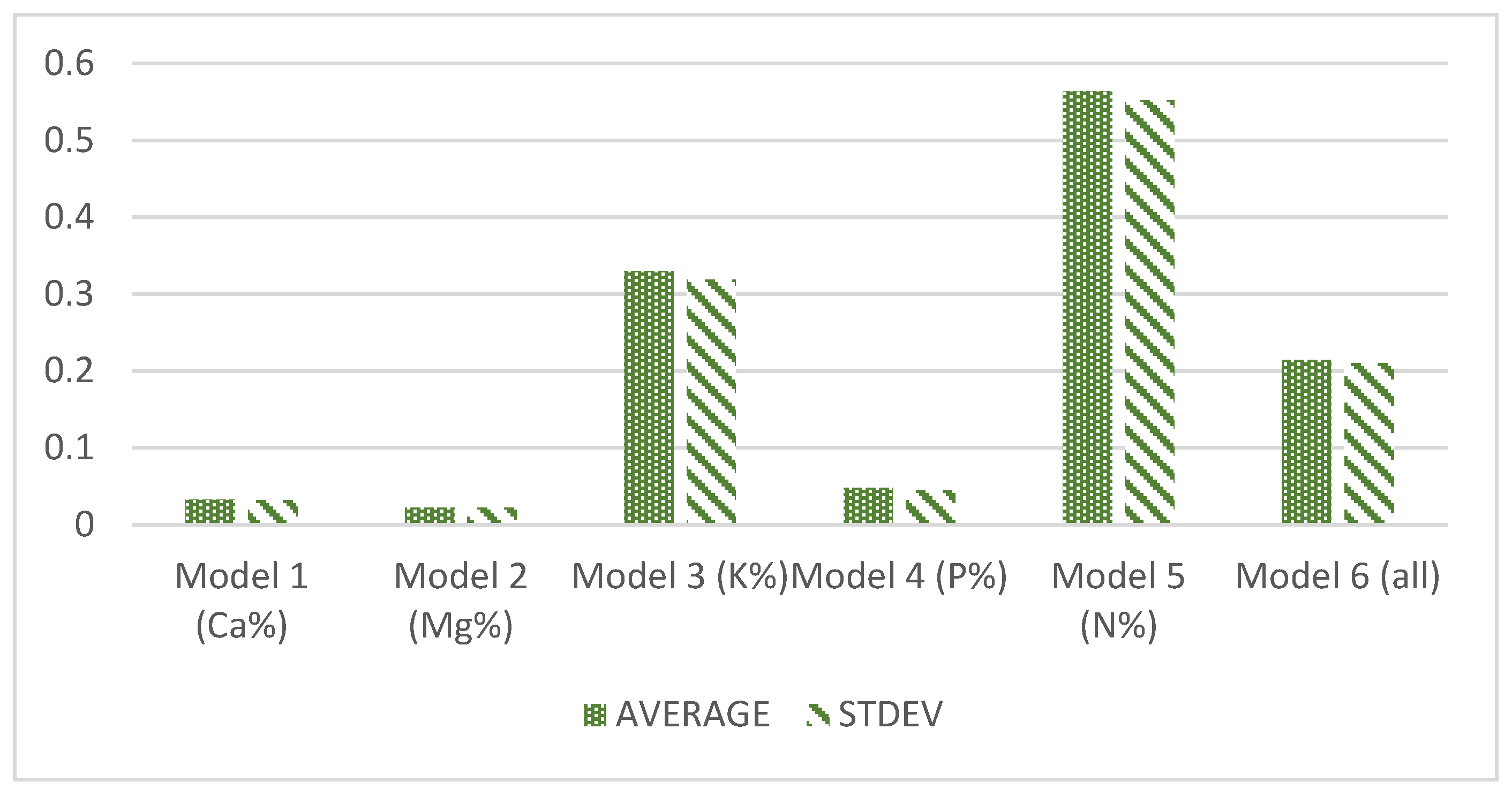
Figure 7.
Features importance for N% nutrient concentration prediction.
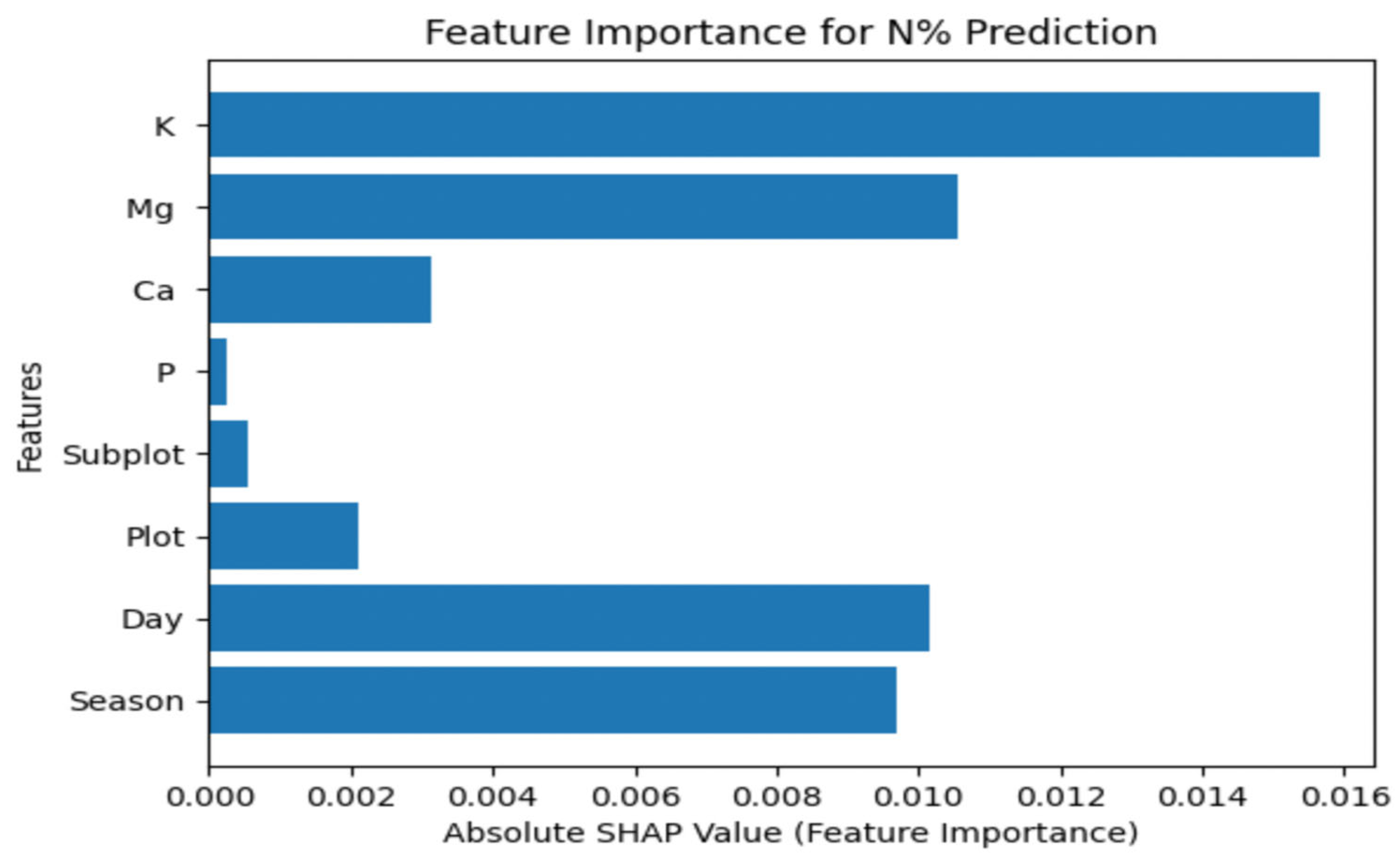

Table 1.
Advantage and disadvantage of linear regression algorithm.
| Linear regression Types | Proficiency | Advantage | Disadvantage |
|---|---|---|---|
| Simple linear regression [13] | Identifying the correlation between two variables | -Computationally efficient -Required less parameters |
-Unable to deal with nonlinearity -Sensitive to outlier |
| Elastic Net Regression [14] | Constructed by combination of Lasso and Ridge regression models. | -Able to deal with large number of features -Prevent overfitting using L1 and L2 regularization methods |
-Computationally expensive -Unsatisfactory results when the number of predictors is more than sample size |
| Polynomial Regression [15] | Captures nonlinearity between variables | -Ability to deal with small dataset | - Computationally expensive -Overfit if the degree of polynomial is high |
| Stepwise Regression [16] | Built by combination of backward and forward selection methods which is beneficial to select best subset of features | -Provide balance between features and algorithms predictive power | -Time demanding -Unstable due to overfitting |
| Ridge Regression [17] | Considered as regularization method | -Able to dela with large dataset -Prevent overfitting |
-Issue with finding optimal value for lambda |
|
Lasso Regression [18] |
Known as regularization method | -Mitigate overfitting | -Challenging while dealing with large dataset that has large number of observations |
Table 2.
Rice dataset descriptions.
| Name of Dataset | Rice Dataset |
|---|---|
| Authorship | --------------- |
| Dataset Characteristics | Multivariate |
| Attribute Characteristics | Categorical Data (Nominal), Numerical & Continual Data |
| Number of Instances | 348 |
| Attributes Number | 9 |
| Missing Values | No |
Table 3.
Nutrient prediction models based on co-existence, composition and concentration.
| Spatiotemporal Factors | Nutrients | ||||||||
|---|---|---|---|---|---|---|---|---|---|
| Model | Season | Day | Plot | Subplot | N (%) | P (%) | K (%) | Mg (%) | Ca (%) |
| 1(Ca%) | Y | Y | Y | Y | Y | Y | Y | Y | N |
| 2(Mg%) | Y | Y | Y | Y | Y | Y | Y | N | Y |
| 3(K%) | Y | Y | Y | Y | Y | Y | N | Y | Y |
| 4(P%) | Y | Y | Y | Y | Y | N | Y | Y | Y |
| 5(N%) | Y | Y | Y | Y | N | Y | Y | Y | Y |
| 6(all) | Y | Y | Y | Y | N | N | N | N | N |
Table 4.
RMSE Performance of Model 1 to Model 6 with Average and STDEV.
| RMSE | ||||||||
|---|---|---|---|---|---|---|---|---|
| Method | Model 1 (Ca%) | Model 2 (Mg%) | Model 3 (K%) | Model 4 (P%) | Model 5 (N%) | Model 6 (all) | AVG | STDEV |
| Elastic Net Regression | 0.0362 | 0.0193 | 0.3991 | 0.0651 | 0.6326 | 0.2376 | 0.2305 | 0.2738 |
| Polynomial Regression | 0.0255 | 0.0395 | 0.1726 | 0.0267 | 0.4866 | 0.1502 | 0.1502 | 0.1979 |
| Stepwise Regression | 0.0357 | 0.0184 | 0.4241 | 0.0497 | 0.5741 | 0.2572 | 0.2204 | 0.2601 |
| Ridge Regression | 0.0345 | 0.0176 | 0.2860 | 0.0402 | 0.5070 | 0.1949 | 0.1771 | 0.2152 |
| Lasso Regression | 0.0297 | 0.0193 | 0.4131 | 0.0651 | 0.6768 | 0.2494 | 0.2408 | 0.2934 |
| Linear Regression | 0.0345 | 0.0175 | 0.2852 | 0.0400 | 0.5056 | 0.1949 | 0.1766 | 0.2146 |
| AVG | 0.0327 | 0.0219 | 0.3300 | 0.0478 | 0.5638 | 0.2140 | ||
| STDEV | 0.0321 | 0.0224 | 0.3185 | 0.0449 | 0.5523 | 0.2101 | ||
Table 5.
Performance of Model 1 to predict Ca%.
| Algorithm | R2 score | MAE | RMSE |
|---|---|---|---|
| Elastic Net Regression | 0.0 | 0.0297 | 0.0362 |
| Polynomial Regression | 0.5017 | 0.0204 | 0.0255 |
| Stepwise Regression | 0.0257 | 0.0292 | 0.0357 |
| Ridge Regression | 0.0869 | 0.0281 | 0.0345 |
| Lasso Regression | 0.0 | 0.0361 | 0.0297 |
| Linear Regression | 0.0931 | 0.0279 | 0.0345 |
| AVG | 0.0 | 0.0297 | 0.0362 |
| STDEV | 0.5017 | 0.0204 | 0.0255 |
Table 6.
Performance of Model 2 to predict Mg%.
| Algorithm | R2 score | MAE | RMSE |
|---|---|---|---|
| Elastic Net Regression | 0.0 | 0.0154 | 0.0193 |
| Polynomial Regression | -3.1900 | 0.0301 | 0.0395 |
| Stepwise Regression | 0.0879 | 0.0151 | 0.0184 |
| Ridge Regression | 0.1734 | 0.0142 | 0.0176 |
| Lasso Regression | 0.0 | 0.0154 | 0.01934 |
| Linear Regression | 0.1742 | 0.0141 | 0.0175 |
| AVG | 0.0 | 0.0154 | 0.0193 |
| STDEV | -3.1900 | 0.0301 | 0.0395 |
Table 7.
Performance of Model 3 to predict K%.
| Algorithm | R2 score | MAE | RMSE |
|---|---|---|---|
| Elastic Net Regression | 0.1967 | 0.3101 | 0.3991 |
| Polynomial Regression | 0.8496 | 0.1275 | 0.1726 |
| Stepwise Regression | 0.0926 | 0.3464 | 0.4241 |
| Ridge Regression | 0.5873 | 0.2266 | 0.2860 |
| Lasso Regression | 0.1391 | 0.3235 | 0.4131 |
| Linear Regression | 0.5895 | 0.2261 | 0.2852 |
| AVG | 0.1967 | 0.3101 | 0.3991 |
| STDEV | 0.8496 | 0.1275 | 0.1726 |
Table 8.
Performance of Model 4 to predict P%.
| Algorithm | R2 score | MAE | RMSE |
|---|---|---|---|
| Elastic Net Regression | 0.0 | 0.0529 | 0.0651 |
| Polynomial Regression | 0.8308 | 0.0212 | 0.0267 |
| Stepwise Regression | 0.4180 | 0.0377 | 0.0497 |
| Ridge Regression | 0.6193 | 0.0311 | 0.0402 |
| Lasso Regression | 0.0 | 0.0529 | 0.0651 |
| Linear Regression | 0.6202 | 0.0312 | 0.040 |
| AVG | 0.0 | 0.0529 | 0.0651 |
| STDEV | 0.8308 | 0.0212 | 0.0267 |
Table 9.
Performance of Model 5 to predict N%.
| Algorithm | R2 score | MAE | RMSE |
|---|---|---|---|
| Elastic Net Regression | 0.3006 | 0.4524 | 0.6326 |
| Polynomial Regression | 0.5862 | 0.3808 | 0.4866 |
| Stepwise Regression | 0.4240 | 0.4388 | 0.5741 |
| Ridge Regression | 0.5508 | 0.3657 | 0.5070 |
| Lasso Regression | 0.1994 | 0.4948 | 0.6768 |
| Linear Regression | 0.5532 | 0.3661 | 0.5056 |
| AVG | 0.3006 | 0.4524 | 0.6326 |
| STDEV | 0.5862 | 0.3808 | 0.4866 |
Table 10.
Performance of Model 6 to predict all nutrients.
| Algorithm | R2 score | MAE | RMSE |
|---|---|---|---|
| Elastic Net Regression | 0.0771 | 0.1814 | 0.2376 |
| Polynomial Regression | 0.5237 | 0.1211 | 0.1502 |
| Stepwise Regression | 0.0450 | 0.2054 | 0.2572 |
| Ridge Regression | 0.3066 | 0.1477 | 0.1949 |
| Lasso Regression | 0.0377 | 0.1918 | 0.2494 |
| Linear Regression | 0.3066 | 0.1477 | 0.1949 |
| AVG | 0.0771 | 0.1814 | 0.2376 |
| STDEV | 0.5237 | 0.1211 | 0.1502 |
Table 11.
ANOVA test for performance analysis.
| Anova: Single Factor | |||||
|---|---|---|---|---|---|
| SUMMARY | |||||
| Groups | Count | Sum | Average | Variance | |
| Model 1 | 6 | 0.1961 | 0.032683333 | 1.77137E-05 | |
| Model 2 | 6 | 0.13164 | 0.02194 | 7.46328E-05 | |
| Model 3 | 6 | 1.9801 | 0.330016667 | 0.009850606 | |
| Model 4 | 6 | 0.2868 | 0.0478 | 0.0002332 | |
| Model 5 | 6 | 3.3827 | 0.563783333 | 0.00603637 | |
| Model 6 | 6 | 1.2842 | 0.214033333 | 0.001695283 | |
| ANOVA | |||||
| Source of Variation | SS | df | MS | F | P-value |
| Between Groups | 1.394 | 5 | 0.2787 | 93.3932 | 2.3253E-17 |
| Within Groups | 0.0895 | 30 | 0.0030 | ||
| Total | 1.4833 | 35 | |||
Disclaimer/Publisher’s Note: The statements, opinions and data contained in all publications are solely those of the individual author(s) and contributor(s) and not of MDPI and/or the editor(s). MDPI and/or the editor(s) disclaim responsibility for any injury to people or property resulting from any ideas, methods, instructions or products referred to in the content. |
© 2023 by the authors. Licensee MDPI, Basel, Switzerland. This article is an open access article distributed under the terms and conditions of the Creative Commons Attribution (CC BY) license (http://creativecommons.org/licenses/by/4.0/).
Copyright: This open access article is published under a Creative Commons CC BY 4.0 license, which permit the free download, distribution, and reuse, provided that the author and preprint are cited in any reuse.


