Preprint
Article

Vibration-Based SHM in the Synthetic Mooring Lines of the Semi-Submersible OO-Star Wind Floater Under Varying Environmental and Operational Conditions

Altmetrics

Downloads

105

Views

32

Comments

0

A peer-reviewed article of this preprint also exists.

Submitted:

21 November 2023

Posted:

22 November 2023

You are already at the latest version

Alerts
Abstract
Synthetic fiber ropes are frequently used as mooring lines in floaters supporting Floating Offshore Wind Turbines (FOWTs) due to their various advantages. Damages in these lines can lead to the disruption of the FOWTs normal operation and thus their early detection is crucial. Currently, this damage detection problem has been investigated exclusively for FOWT chain mooring lines. This study focuses on the damage detection in FOWT synthetic mooring lines under varying environmental-operational conditions (EOCs) via two types of vibration-based Structural Health Monitoring methods: those based on Multiple Models and those based on a single Functional Model. The methods are based on multivariate AutoRegressive or on scalar Transmittance Function (TF) AutoRegressive with eXogenous input models. All methods are evaluated through a Monte Carlo study involving 390 simulations with a 10MW wind turbine mounted on the semi-submersible OO-Star wind floater and two damage scenarios (10%, 14% stiffness reduction) to a single mooring line. The results using acceleration signals from only two measuring positions on the mooring line, indicate the great potential for robust SHM in FOWTs synthetic mooring lines with the TF model-based methods successfully detecting the considered early stage damage scenarios, even for EOCs not encountered in the methods training.
Keywords: 
Subject: Engineering  -   Marine Engineering

1. Introduction

1.1. The General Problem

The offshore wind energy sector is undoubtably undergoing an unprecedented growth, with projections indicating substantial expansion in the coming years. As nations strive to reduce carbon emissions, offshore wind power has emerged as an essential solution for coastal countries. The European Union has set new targets, aiming to achieve 111 GW offshore wind capacity by 2030 and a staggering 317 GW by 2050, surpassing the already ambitious goals of 60 GW and 300 GW set in November 2020 [1]. Similarly, the United States of America have established policies with the goal of installing 30 GW offshore wind power by 2030 [2], while within Asia, China alone targets for 200 GW by 2030 [3]. For the effective achievement of these ambitious targets and the alignment with the global goals for net-zero emissions by 2050, the acceleration of the annual deployment rate of offshore wind projects is crucial [4]. Yet, the offshore wind industry faces significant challenges, which include not only the total lifecycle costs of the turbines themselves but also the inherent risks associated with these substantial investments.
The operational and maintenance (O&M) cost plays a pivotal role in the overall offshore wind turbine life expenses, comprising a range of 13.9% to 19.6% of the levelized cost of energy (LCOE) [5,6]. Among these costs, the maintenance strategy itself is a major factor. Evidently, the utilization of corrective maintenance, which involves addressing issues as they occur, is not a sustainable approach for offshore wind turbines, due to the substantial ramifications of prolonged downtimes [7]. Preventive maintenance schemes, which depend on frequent inspections aimed at addressing issues before they lead to failure, hold the potential to mitigate these maintenance-related downtimes; however, the harsh oceanic conditions limit the available time windows for on-site inspections, extending the periods between them. Consequently, more time is allowed for damages to develop into an irreparable level before being detected [7]. Moreover, planned on-site inspections demand considerable downtime, as many of them cannot be conducted while the turbine is operational. Finally, given that floating wind turbines can be situated to well over a hundred kilometers from the shore (e.g., the Hywind Tampen wind farm, locate in the Norwegian North Sea [8]), the transportation cost for the inspections are also substantial. These challenges can be mitigated with condition-based maintenance strategies, which involve the continuous remote measurement of relevant information regarding the structural state, as well as the utilization of Structural Health Monitoring (SHM) techniques for damage detection [9].
A critical part of Floating Offshore Wind Turbines (FOWTs) that requires monitoring is the mooring lines, as their failure may lead to several catastrophic events [10]. Firstly, such failure will result in a drift, disconnecting the electric cable, jeopardizing the power production, and introducing the risk of collision with other wind turbines. Furthermore, the stability of the structure itself can be compromised, resulting in increased oscillations, subjecting other critical components to additional stress [11], and potentially leading to capsizing ore even sinking. It becomes evident that maintaining an up-to-date understanding of the mooring line conditions is essential for preventing these dire consequences.
When it comes to deep-sea installations, conventional chain or steel wire are not appropriate options for the mooring system since, with increasing depth, the weight of the mooring line alone exceeds its stress limit. Synthetic fiber ropes are advantageous in this regard, as their density is comparable to water’s, allowing for neutral buoyancy and therefore rendering them suitable for any depth [9]. Furthermore, they possess greater fatigue and corrosion resistance, which are significant design factors in the corrosive and dynamically loaded offshore environment [12]. Nonetheless, these advantages come with some challenges when it comes to the lines’ monitoring.
Usually, mooring lines are monitored through visual inspections using Remote Operated Vehicles (ROVs). Although this approach may be suitable for monitoring chains or steel wires, it is not for synthetic mooring lines. This is because the complex composition of synthetic ropes and their jacket, if present, hinders potential damage in the internal strands [13] (see Figure 1). Furthermore, biofouling and murky water might also obstruct reliable visual inspection. Therefore, alternative methods of monitoring must be employed.
For the monitoring of synthetic mooring lines, vibration-based methods constitute a fitting choice due to their several advantages [14]. Firstly, they possess the potential to detect a wide range of damages, including those which may not be visible from the outside of the jacket. Additionally, these methods are cost-effective in terms of instrumentation and operation, as they require only a small number of sensors. The sensors, typically accelerometers, can be easily placed on the jacket's exterior, avoiding interference with the rope's structure and its properties, unlike embedded technologies (e.g., optical fibers) [15]. Furthermore, they do not require presence of personnel on the wind farm, enabling real-time inspection and reducing transportation costs and occupational risks. Finally, these methods can be extended for damage identification, quantification, localization, and estimation of the remaining service life of the rope, depending on the availability of signals from damaged cases.
Despite their advantages, vibration-based methods do present some challenges, with the most prominent one being their sensitivity to uncertainties, particularly those posed by varying Environmental and Operational Conditions (EOCs). This sensitivity may result in a high rate of false alarms, rendering them impractical.
To the best of the authors' knowledge, the existing literature on vibration-based SHM for mooring lines in FOWTs is very limited. In [16], a deep Neural Network (NN) method is employed to detect structural changes in a semi-submersible floater based FOWT due to biofouling in chain mooring lines. [17] proposes a fuzzy logic-based method for the detection, identification and quantification of stiffness reduction in the mooring lines of a Tension Leg Platform (TLP) floater based and Spar floater based FOWT. [18] introduces a non-probabilistic method utilizing artificial NNs to detect and identify stiffness reduction in the mooring lines of a semi-submersible floater based FOWT. In [19], a Power Spectral Density (PSD) based method is used for the detection and identification of damages at the fairlead and the anchor of a semi-submersible floater based FOWT with a combination of chain and synthetic mooring lines. In [17,18], the type of the mooring line is not clarified. Based on the above, damage detection in synthetic mooring lines of FOWTs has not been investigated. Additionally, no varying EOCs are considered in [17,18] whereas in [19], it is not clear how the varying EOCs are used in the training of the PSD-based method, while no healthy scenarios are examined during the method’s evaluation. Finally, the same EOCs are considered in the training and the evaluation of the NN-based method presented in [16]. The current study aims to address the above-mentioned open issues through robust vibration based SHM methods for damage detection in a FOWT’s synthetic mooring lines.

1.2. Conceptual Approach: Mitigating Uncertainties in Vibration-Based SHM

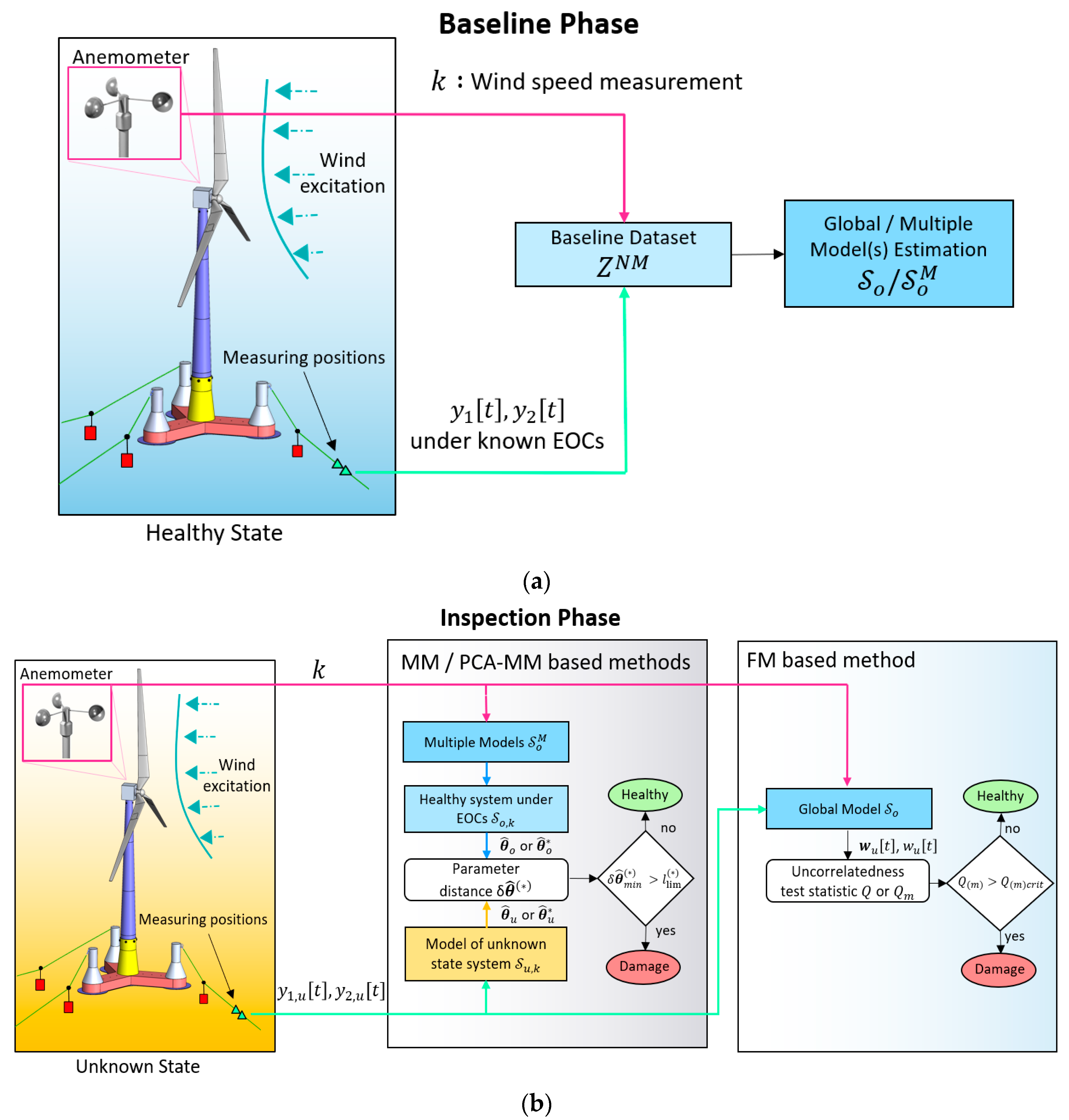
Vibration-based data-driven SHM methods consist of two phases: the training also known as baseline phase, and the inspection phase. In the training phase which is performed once, signals obtained under the healthy state of the examined structure are used for the estimation of one or more baseline (nonparametric/parametric) data-driven models that represent the structural dynamics under varying EOCs and other uncer-tainty. During the inspection phase, which is performed periodically or on demand in real time, the health state of the mooring lines is unknown and is determined using vibration signals for the identification of similar models as those used in the baseline for the healthy mooring lines. If the current models deviate significantly from their baseline counterparts implies that the lines dynamics has been significantly altered due to an induced damage.
There are several types of data-driven models which are used for the representa-tion of the structural dynamics [20,21,22] (pp. 79-139). The use of parametric stochastic models of the AutoRegressive–Moving Average with eXogenous (ARMAX) input fam-ily, is a popular choice due to their formulation, which allows their parameters to be directly associated with the dynamic characteristics (i.e., natural frequencies and damping ratios) of the considered structure. This is a notable difference from many data-driven methods that treat the vibration signals (and thus the structural dynamics) as some inputs to artificial NNs [16,18] without engineering explainability and inter-pretability.
Vibration-based methods can be classified into input-output or output-only, de-pending on the availability of the excitation signal. Input-output methods usually rely on the deliberate excitation of the structure using mechanical actuators, enabling better control over the excitation frequency bandwidth and energy. Thus, the obtained vibra-tion response(s) provides detailed information about the structural dynamics across the entire, selected, spectrum leading to a more accurate evaluation of the structural con-dition comparing with output-only methods where the excitation is unknown. Such methods usually utilize ARX models, which additionally with the measured vibration response(s) incorporates the excitation [21,22] (pp. 81-83). On the other hand, the output-only methods rely exclusively on vibration response signals from the considered structure as these are acquired under ambient, unknown, excitation, rendering them suitable for cases where the use of a mechanical actuator is expensive or impractical. However, the trade-off for this practical facilitation is that the frequency content of the measured vibration signals and thus the investigation of the structural dynamics, is limited by the excitation bandwidth, which typically includes reduced information at lower frequencies especially when physical excitations such as wind and waves are considered.
One way to reduce the impact of excitation variability to structural dynamics that may mask similar effects due to an early-stage damage and thus increase SHM effectiveness, while adhering to response-only type methods, is by using the vibration signals Transmittance Function (TF) [23]. The TF is defined as the ratio of the Cross-Spectral Density (CSD) over the Power (auto)-Spectral Density (PSD) of two response signals, y 1 t and y 2 t , measured at different positions on the structure [23]:
T j ω = S y 2 y 1 j ω S y 1 y 1 ω  
where ω designates frequency, j the imaginary unit, S y 2 y 1 the CSD of y 1 t and   y 2 t , and S y 1 y 1 the PSD of y 1 t .
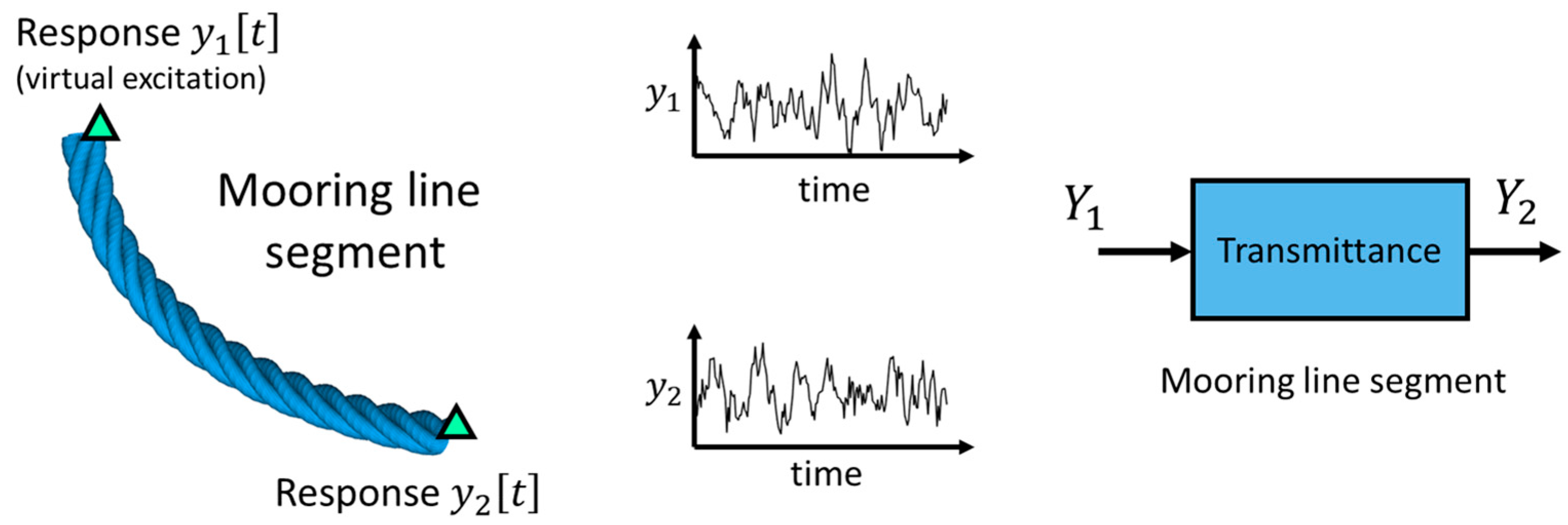
The TF resembles a typical Frequency Response Function (FRF), with the distinction that two separate output signals are used instead of a pair of input-output signals. To facilitate a better understanding of the TF functionality within the specific context of the current study, Figure 2 illustrates its application in modeling a mooring line segment. As depicted in the figure, two response signals are measured using accelerometers, one at each side of the segment. By designating one of the two measured signals as the excitation and the other as a response, it becomes possible to define a system representing the relative admittance between the two measuring positions. The underlying idea for its application is that, akin to a conventional FRF, the TF remain unaffected by the excitation variability, yet exhibit high sensitivity to damage.
The TF similarity with the FRF also allows for the parametric ARX (TF-ARX) representation of the TF [23], providing a different approach when multiple signals are available, in addition to the Vector-AR (VAR) stochastic models [22] (pp. 91-93), [24,25].
EOCs play a significant role in the system dynamics. A conventional data-driven model of any of the ARMA, Vector ARMA, (VARMA) and ARMAX types can represent the healthy structural state under a single EOC. Hence, a different approach is necessary for accommodating variations in the EOCs and preventing their misinterpretation that may lead to increased false alarms or missed early-stage damages. Such an approach can be founded upon two main concepts. The first involves the use of implicit methods such as the Factor Analysis (FA) [26] and Principal Components Analysis (PCA) based methods [27], which extract features from the vibration signals that are exclusively sensitive to damage and not to the EOCs. The second concept involves the use of explicit methods such as the Multiple Model (MM) based ones [27,28] and the Functional Model (FM) based methods [29,30], where the influence of the EOCs is incorporated in the models representing the healthy structural dynamics.

1.3. Aim and Objectives

As it is mentioned in section 1.1, the literature about damage detection in FOWT’s mooring lines is very limited with the focus being on chain mooring lines, while damage detection in FOWTs’ synthetic mooring lines is still unexplored. Thus, the aim of the present study is to investigate this problem via the following robust vibration-based SHM methods which are capable of mitigating the challenge of the varying EOCs and other uncertainty sources that may significantly affect the structural dynamics and mask potential effects due to early stage damages leading to unreliable damage detection.
  • Multiple Model (MM) based methods
  • PCA variants of the MM methods
  • Functional Model (FM) based methods
The employed methods are based on either VAR or on scalar TF-ARX data-driven models, thus they are abbreviated as MM-VAR, MM-TF-ARX, FM-VAR and FM-TF-ARX, while the PCA variants of the first two methods are designated as PCA-MM- -VAR and PCA-MM--TF-ARX.
These methods are evaluated and compared through hundreds of Monte-Carlo simulations conducted via the finite element model of a 10MW FOWT supported by the semi-submersible OO-Star Wind Floater. Two damage scenarios corresponding to 10% and 14% stiffness reduction are performed to a single mooring line. Damage detection is based on acceleration signals from a limited number of measuring positions with the optimum positions selected via PSD based and TF based criteria.
The remainder of the article is organized as follows: Section 2 provides an overview of the FOWT, the Monte-Carlo simulations, and a comparative analysis of the changes in the system dynamics resulting from damage in a mooring line and changes in EOCs. Additionally, this section presents a systematic approach for selecting the optimal measuring positions for damage detection based on specific criteria. In Section 3 the MM, PCA-based MM, and FM-based methods’ framework is introduced, along with the models employed within them. Section 4 provides the system identification process, and the results of the detection methods are presented. These results are subsequently reviewed in Section 5 and conclusions are provided in Section 6. Preliminary results of this study based on scalar models have been presented in a conference paper [31].

2. Case Study

2.1. The 10MW FOWT supported by the semi-submersible OO-Star wind floater

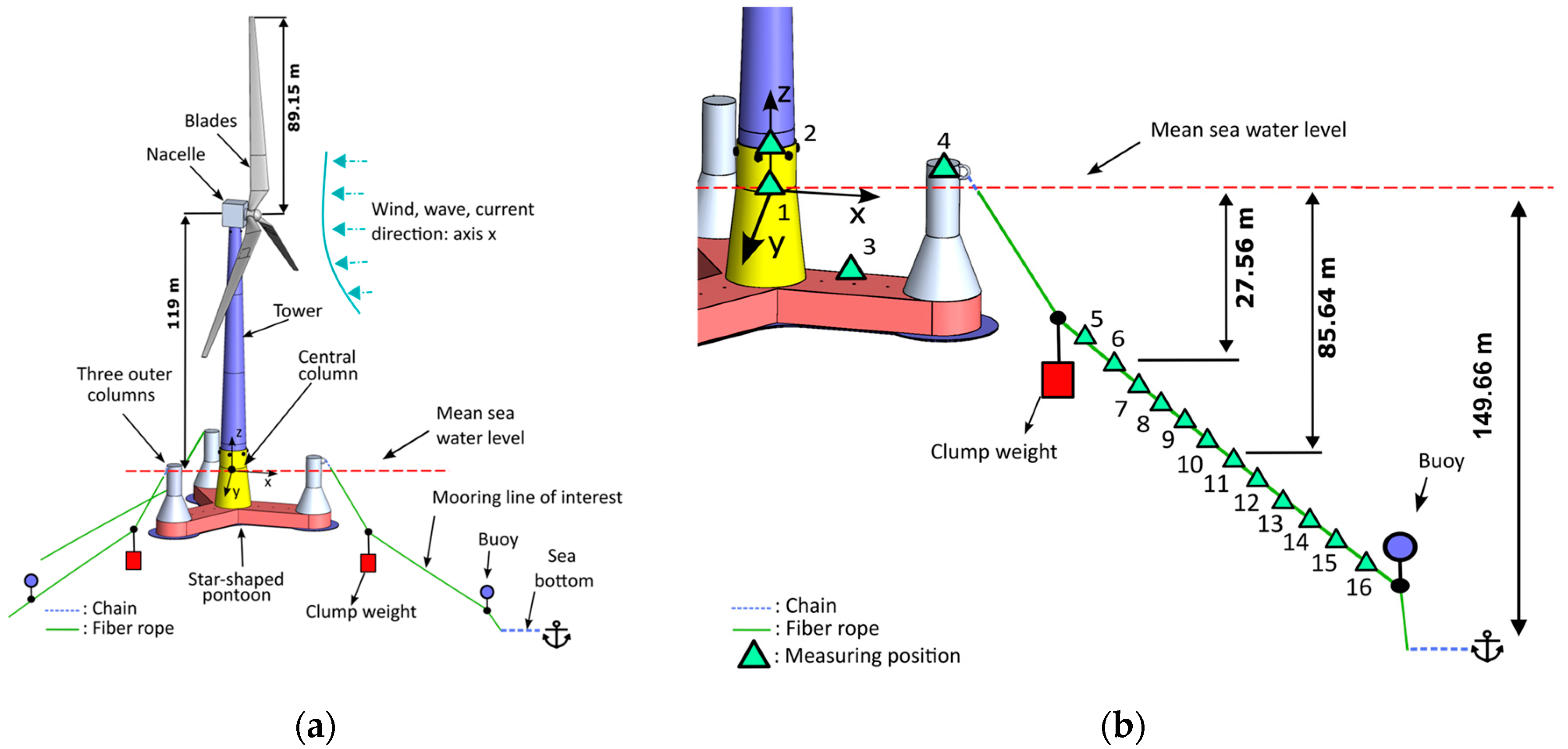
The case study for the implemented methods involves a simulation model of a 10 MW Reference Wind Turbine mounted on the semi-submersible OO-Star floater which is designed by Dr. techn. Olav Olsen AS (DOOA) [33,34] and developed in the Technical University of Denmark (DTU) [32]. As illustrated in Figure 3a, the substructure is composed of four columns, three outer and one central, interconnected with a star-shaped pontoon. The central column provides support for the wind turbine, while the outer columns contribute to the overall stability of the structure. The entire substructure is constructed from post-tensioned concrete and is secured in position using a semi-taut mooring system, consisting of three lines attached to the top section of the outer columns. Each mooring line is primarily composed of synthetic rope except for the bottom part, which is in contact with the seabed, and a small segment at the connection with the substructure, both of which are composed of steel chain. At a specific point on each mooring line close to the surface, a clump weight is placed to enhance the substructure’s restoring forces, thereby reducing its vertical offset. Furthermore, a buoy is attached to each line, positioned between the synthetic rope and the steel chain segments, with the primary function of preventing the synthetic rope from making direct contact with the seabed.
The examined substructure presents several advantages, which makes it a compelling option for renewable energy production. Firstly, the semi-submersible substructure can be manufactured and assembled alongside the wind turbine off-site and then towed to its designated location, avoiding the additional costs and risks associated with complex on-site installation. In the case of utility-scale wind turbines, the transportation of their components on the assembly location is also a significant concern. Concrete as a material is advantageous in this regard because it can be easily transported directly to the construction site in its raw form [35]. Furthermore, it has higher local availability than steel, given that most countries have one or several cement producers. Additionally, concrete has a lower cost than steel, while also exhibiting higher corrosion resistance, lower operation and maintenance costs, and a longer design life [36].
The OO-Star floater has been investigated extensively within the LIFES50+ [33,37] and FLAGSHIP [34] projects and is now owned by Bouygues Travaux Publics.

2.2. The Monte-Carlo simulations

The vibration signals used for the evaluation of the implemented SHM methods are obtained from Monte-Carlo simulations conducted through the aero-hydro-servo-elastic simulation tool 3DFloat, developed by the Institute of Energy and Technology (IFE) [38]. This tool uses a Finite Element Model (FEM) with 2706 Degrees of Freedom (DoF), created jointly by DOOA and IFE. During the Monte-Carlo simulations, the operating wind turbine is subjected to stochastic wind excitation generated following the Kaimal spectrum model [39](p. 30), while waves are generated following the JONSWAP spectrum [40]. To calculate the structure's response with 3DFloat, the equations are formulated at each time step in a coordinate system attached to a reference configuration, which is a deformed state from the previous time step. This approach enables the use of small-strain elements to accommodate significant global deflections, thereby accounting for geometric nonlinearities. The outputs of 3DFloat may include motions, stresses, and other types of signals regarding the operating system.
The SHM methods evaluated in the present study make use of acceleration signals. Multiple measuring positions are considered both along the mooring line and on the substructure, as depicted in Figure 3b. For each position, one signal is produced, corresponding to the x direction where the excitation is applied. The sampling frequency is selected to be f s = 5 Hz, based on the low frequency wind and wave excitation [37]. Details regarding the simulated cases are shown in Table 1 and discussed in subsections 2.3 – 2.5.

2.3. The Damage Scenarios

Throughout their lifespan, synthetic rope mooring lines are vulnerable to several damage modes that require attentive monitoring [13,15]. During regular operation, the rope experiences cyclic loading, which over time results in tensile and compression fatigue. The primary mechanism of tensile fatigue is the internal fiber-on-fiber abrasion caused by the rubbing of strands within the rope (see Figure 1). This continuous friction eventually leads to the breaking of the rope's yarns. Compression fatigue on the other hand happens when the strands buckle or kink under compression, resulting in a reduction of the fibers’ strength and allowing for increased inter-yarn movement, which, in turn, leads to more abrasion [15]. Overloading or shock due to extreme weather conditions, ship or trawl collisions, and seismic events are also relevant damage modes that can result in significant strength loss or even fracture. Finally, when a rope is subjected to constant load over a long period of time, its length is increased, a phenomenon also known as creep. If the period is long enough, this elongation becomes irreversible, altering the molecular polymer chains and eventually leading to an increase of stress that accelerates into failure [15].
The above damage modes depend on the stress and/or deformation profile of the line. Cycling loading occurs throughout the entire length of the rope, although certain regions that experience higher load amplitudes are expected to be more affected by tensile fatigue. Regions which operate in lower tension during the alternate loading are on the other hand more likely to buckle and thereby undergo compression fatigue, while sections subjected to constant static loading are more likely to undergo substantial creep, depending on the fiber material [15]. The determination of the degradation's distribution along the line's length is a challenging task. It depends not only on the spatial and temporal stress profile of the line but also on the influence of each damage mechanism, the quantification of which is itself dependent on many factors. However, such an analysis falls out of the scope of this study, and a uniform degradation is herein adopted as in [17,18] where 10% and 20% reduction in the stiffness of the mooring lines, characterized as light, is considered. In particular, the detection of two early stage damage scenarios, corresponding to stiffness reduction of 10% and 14% along the entire length of the synthetic rope, are investigated in the current study.
It is important to note that one of the major challenges associated with synthetic mooring lines is their handling during installation, as synthetic ropes are susceptible to damage when mishandled by contractors operating on tight time schedules. Although identifying initial weaknesses in the mooring systems is also of significant interest, this study exclusively focuses on damages that might occur in the ropes after an initial period of operation. Therefore, it is assumed that during this initial period of operation, the mooring lines remain in a healthy state.

2.4. The Environmental and Operational Conditions

As stated before, the EOCs have a significant impact on the structural dynamics. Wind speed, direction, wave height, temperature, and other environmental factors are important sources of uncertainty that should be considered when assessing the robustness of vibration based SHM methods. In the current study, uncertainty is introduced to the dynamics by considering different mean wind speed values   U ¯ h u b , measured at hub height (see Figure 3a), within the 7 m/s – 12 m/s range. The significant wave height H s and peak period T p are also treated as variables, dependent directly on the wind speed, as depicted on Table 2.

2.5. Influence of the EOCs and Damage on the structural dynamics

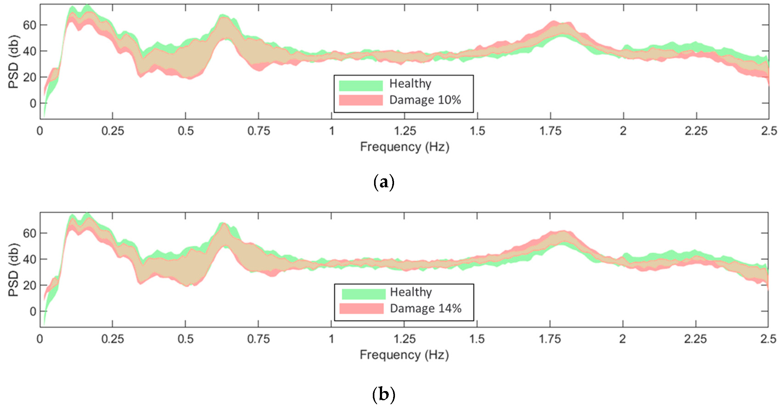
The challenge addressed in the current study is demonstrated by comparing the effects of EOCs on the FOWT dynamics with those of the induced damages. This comparison is illustrated in Figure 4, through the non-parametric PSD estimates of acceleration signals corresponding to an indicative measuring position, specifically, position 11 of the mooring line in the x direction (see Figure 3b). In the figure, the green area corresponds to the healthy state under the EOCs specified in Table 2, while the red areas correspond to the damaged states with damage levels of 10% and 14%, also under varying EOCs. The challenge in the damage detection problem lies in the difficulty of distinguishing whether the measured dynamics of a signal under an unknown state corresponds to the healthy (green area) or the damaged state (red area).
The PSD reflects the underlined FOWT structural dynamics due to the stochastic wind and wave excitation. Changes in the frequency content of the excitation sources will accordingly affect the structural dynamics and thus the frequency content of the obtained vibration signals. Therefore, such variations in wind speed and wave excitations will have a significant impact on the PSD, even if the structure remains healthy. As previously discussed, employing the TF can mitigate such excitation variability on the structural dynamics, which may be responsible for high rates of false alarms. The use of TF necessitates good coherence between the employed signals, with values close to unity, indicating low signal to noise ratio and measurement errors as well as weak nonlinear or time-variant behavior of the structure [41](pp. 20,135):
C ω = S y 2 y 1 j ω 2 S y 1 y 1 ω S y 2 y 2 ω  
To verify that the TF can be used, the coherence function is assessed for each possible combination of measuring positions. The position combinations with the best coherence function values are shown in Figure 5. It is worth noting that a relatively good coherence is observed only among responses in the x direction and between adjacent measuring positions. This can be attributed to the direction of the structure’s excitation in relation to the mooring line topology (see Figure 3a) and the closeness of the adjacent measuring positions (Figure 3b). As shown in Figure 3a, the mooring line under examination extends in the x-direction, which is aligned with the wind and wave propagation. This alignment results in heightened vibrations in this specific direction. For neighboring sensor positions in the x direction, the coherence demonstrates favorable values, except within the frequency range of [2.2 - 2.5] Hz. These low values are attributed to the low pass filter applied during signal sampling, which attenuates the spectra in this specific frequency range.
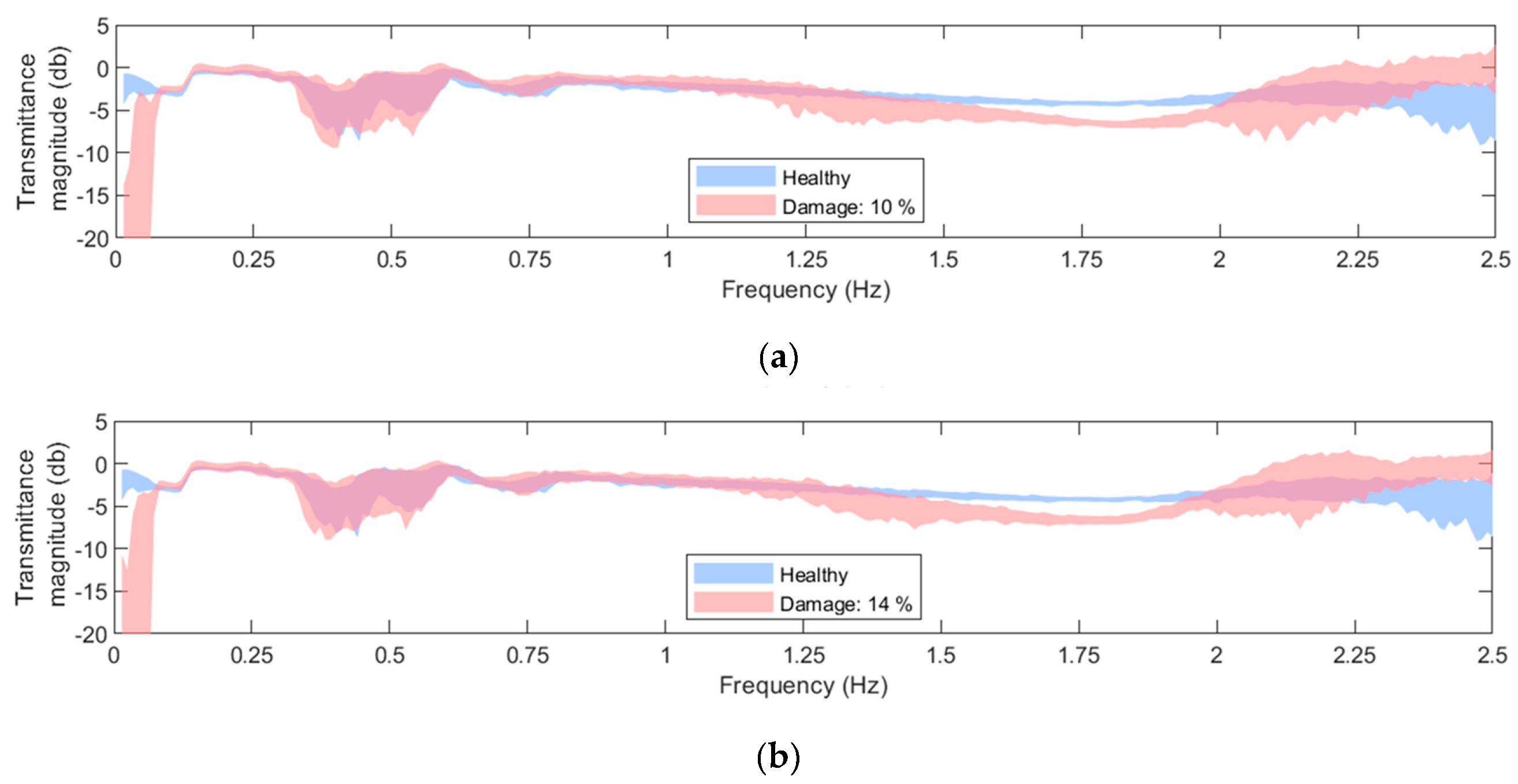
Figure 6 illustrates the sensitivity of the TF to damage. When compared to the PSD (see Figure 4), it appears that the TF may be more noticeably affected by the considered damage, specifically in the bandwidth of [1.5 - 2] Hz.
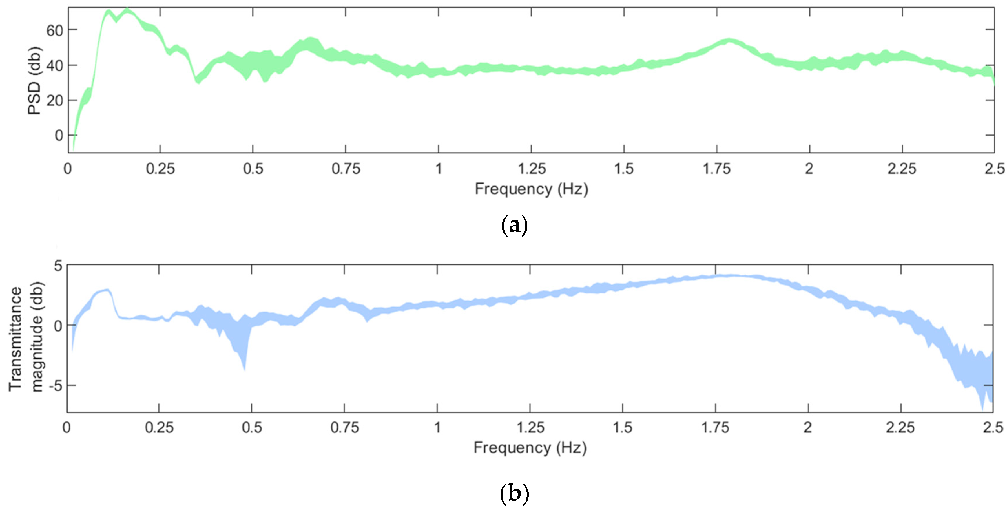
In addition to the variability of U ¯ h u b , H s , and T p , the stochastic nature of wind and wave excitations is also a source of uncertainty. In this simulated model, this uncertainty is addressed by employing various random seeds in the pseudorandom generation of the wind and wave excitations. The influence of this uncertainty is highlighted in Figure 7 where the PSD and the TF are depicted for a specific case but using different realizations. In the context of this study, the stochasticity of the wind and wave excitations is taken into account by utilizing multiple signals produced during the simulations based on different random seeds.

2.6. Selection of the measuring positions

One of the key considerations for selecting SHM methods is the instrumentation and installation cost. In this context, vibration-based methods have an advantage as they require a relatively small number of sensors when they are strategically placed. In the current study, the optimal measuring positions are determined by evaluating the sensitivity of the response signals’ PSD and TF to damage. This is achieved through the Frequency Response Assurance Criterion ( F R A C ), the Frequency Amplitude Assurance Criterion ( F A A C ) and the average Local Amplitude Criterion ( L A C ¯ ) [29].
F R A C = h o T h d 2 h o T h o h d T h d
F A A C = 2 h o T h d h o T h o + h d T h d
L A C ¯ = 1 n ω i = 1 n ω 2 H o * j ω i H d j ω i H o * j ω i H o j ω i + H d * j ω i H d j ω i  
with o and d the subscripts designating the healthy and damaged states respectively, T and * as superscripts indicating matrix or vector transpose and complex conjugation respectively, · the magnitude of a complex quantity, H j ω i the PSD or TF at frequency ω i , h a vector consisting of the PSD or TF for successive (discrete) frequencies (vectors are indicated by lowercase boldface, and matrices by uppercase boldface symbols) and n ω the number of the employed discrete frequencies. The values of these criteria serve as indicators of sensitivity to damage, with the most sensitive measuring positions being those that yield the F R A C , F A A C , and L A C ¯ values with the highest deviation from the unit. From the above equations, each value of F R A C , F A A C and L A C ¯ is calculated using the PSDs or TFs of a single pair of healthy h o and damaged h d states.
In the current study, considering the uncertainty arising from varying EOCs, the optimal sensor positions are determined by evaluating the mean value of each criterion which is calculated based on 1200 combinations are the sum of 6 batches of combinations of healthy and damage cases, one batch for each U ¯ h u b value of   7 ,   8 ,   9 ,   10 ,   11 and 12 m/s. Each of batch includes 200 combinations of healthy and damage cases and it is based on ten healthy cases and 20 damage cases, with the latter corresponding to 10 cases for each of the damage levels 10% and 14 %. Each simulation is conducted under a different random seed and n ω =   88 is based on the considered frequency bandwidth 1 ,   2.25   H z and a frequency resolution of 0.0143 Hz. The Welch estimate of the PSDs and TFs used in the criteria calculations is based on Hamming Window, window size: 350; f s   = 5 Hz; sample size N = 8500 ; overlap: 95%.
From Figure 4 and Figure 6, it is evident that frequencies below 1 Hz exhibit relatively low sensitivity to damage in both the PSD and TF. On the other hand, these frequencies show a high level of variability due to changes in EOCs. This is why it is decided PSD and TF values only within bandwidth of 1 ,   2.25   H z to be used for the calculation of the criteria.
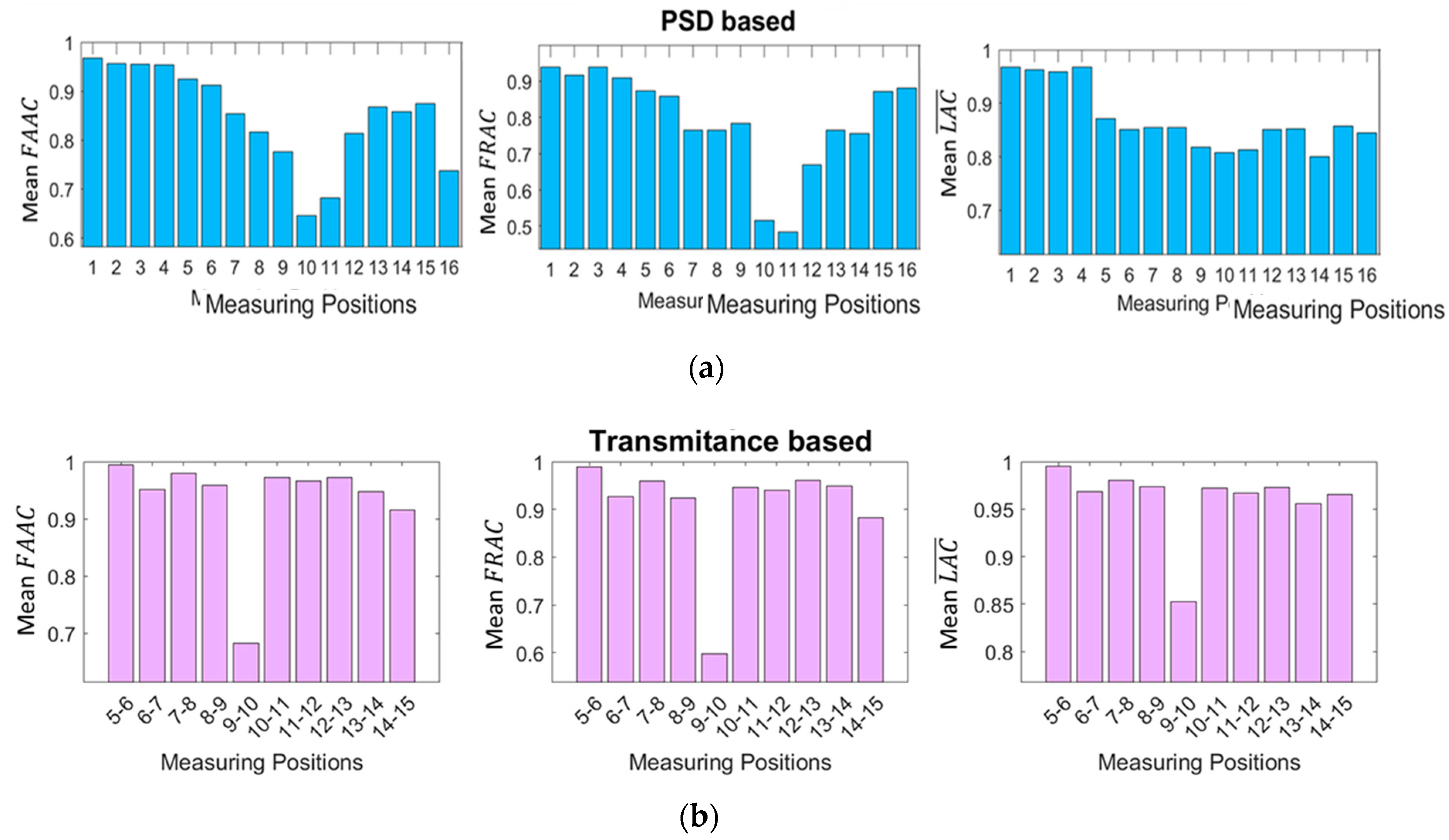
Figure 8a shows the criteria values based on the PSD for every considered measuring position in the x direction, while Figure 8b shows the mean criteria values based on the TF function for the adjacent responses in the x direction as well. Based on the PSD, only F A A C and F R A C agree on the 10 and 11 positions in the x direction where the excitation applies, while based on the TF, all three criteria confirm that the highest sensitivity to damages is given by the combination of positions 9 – 10 in the x direction.

3. Damage Detection Methodology

The current section includes a description of the baseline and inspection phases of the evaluated SHM methods. Six methods are employed: two MM-based methods, two PCA-based MM methods, and two FM-based methods. The MM-based methods [28] are employed using VAR models [22](pp. 91-93) for the representation of the structural dynamics, abbreviated as MM-VAR, or using TF-ARX [23] models, abbreviated as MM-TF-ARX. The PCA based MM methods, abbreviated as PCA-MM, correspond to the MM-based methods with PCA parameter reduction before the detection process [28]. Thus, two variants of the PCA-MM methods are examined, the PCA-MM-VAR and the PCA-MM-TF-ARX. Additionally, the FM-based methods [29,30,42,43,44] are employed, utilizing either an FP-VAR model [44] and abbreviated as FM-VAR or an FP-TF-ARX model [30,43], abbreviated as FM-TF-ARX. All six methods are trained using pairs of signals that are collected under healthy FOWT normal operation with varying EOCs during the baseline phase (see Table 1). It is noted that the varying EOCs characterized by U ¯ h u b (also see section 2.3), are measurable in both baseline and inspection phases.

3.1. Baseline/ Training Phase

During the training phase of the methods, where the FOWT is under healthy state, M pairs of acceleration signals y t = y 1 t   y 2 t Τ ,   t = 1,2 , N are acquired from two measurement points for a sample of U ¯ h u b   values; bold upper case symbols designate matrix quantities, bold lower case symbols designate column-vector quantities and T designates transposition. Thus, k = U ¯ h u b indicating a distinct operating condition is defined and normalized in the range of k 0,1 , with each discrete value k i   k 1 , k 2 , , k M being assigned to a corresponding pair of measured signals. The complete baseline dataset can therefore be designated as [42]:
Z N M y 1 , k i t , y 2 , k i t     ,   k i { k 1 ,   k 2 ,   ,   k M } }
This dataset is collected from the healthy structure for a sample of U ¯ h u b values within the range of interest.

3.1.1. Multiple Models (MM) Based Methods

In the MM-based methods, an equal number to M models are estimated based on the acquired pairs of signals [27,28]:
S o M S o , k i   k i k 1 ,   k 2 ,   ,   k M }
The VAR and TF-ARX models used in the MM-based methods are concisely presented in the following.
VAR model:
A two-response VAR model can be expressed as [22](pp.91-93), [45](pp. 4-5):
y t +   τ = 1 n a A τ · y t τ = w t ,   w t ~ i i d   N 0 , Σ w , E w t · w T t τ =   Σ w · δ τ ,
where n a designates the model order, A τ the model [2×2] parameter matrix, E · statistical expectation, w t = w 1 t   w 2 t T a [2×1] vector including zero-mean residual (white noise) signals which follow an identically independent (iid) normal distribution N 0 , Σ w with [2×2] covariance matrix Σ w and δ τ the Kronecker delta ( δ τ = 1   for τ = 0 and δ τ = 0 for τ 0   ). Rearranging the model’s parameters into a 4 n a × 1 parameter vector [45](p. 70) leads to:
θ = v e c A 1 A 2 A n a T
where v e c · signifies vectorization. An estimation of the VAR model (equation (6)) for each k i can be obtained using the ordinary least square (OLS) estimator [22](pp. 203-207, 545-546), [45](pp. 69-72):
θ ^ = Φ Τ Φ 1 · Φ Τ y
where   ^ designates estimate or estimator, y = y 1 y N T the 2 N × 1 response signal for t = 1 ,   , N and Φ the model’s 2 N × 4 n a regression matrix including the acceleration signals; see more details about the construction of Φ in [22](pp. 545-546). Having estimated the parameters of the model, the estimated residual signals (one-step ahead prediction errors) w t , θ ^ can be obtained based on equation (8) [45](p. 94). It is worth emphasizing that w t , θ ^ approximate a white noise only if the model can accurately represent the structural dynamics. The residual signals’ uncorrelatedness can therefore be assessed to validate the estimated model. The 4 n a × 4 n a covariance matrix of the estimated parameters is given by [45] (p. 74):
Σ ^ θ = Σ ^ w Φ Τ Φ 1
where Σ ^ w is the covariance matrix of w t , θ ^ and the Kronecker product.
TF-ARX model:
A TF-ARX model can be expressed as [23]:
y 2 t + τ = 1 n a a τ · y 2 t τ = τ = 0 n b b τ · y 1 t τ + w t ,   w t ~ i i d   N 0 , σ w 2 , E w t · w T t τ = σ w 2 · δ τ
where n a , n b the AR and X orders of the model, a τ and b τ the AR and X parameters and w t a zero-mean residual (white noise) signal which follows an iid normal distribution N 0 , σ w 2 distribution with variance σ w 2 . The parameter estimation for TF-ARX is performed using typical OLS [22], with θ the model n a + n b + 1 × 1 parameter vector and Φ the corresponding N × n a + n b + 1 regression matrix. The estimated parameters covariance matrix is in this case given by [22](pp. 551-553):
Σ ^ θ = σ ^ w 2 · Φ Τ Φ 1
with σ ^ w 2 , the variance of the estimated residual signal w t , θ ^ .
By estimating one model for each k i , a collection of parameter vectors θ ^ k i is obtained. This collection forms a discrete subspace [28] that represents the dynamics of the healthy structure under the different EOCs corresponding to the baseline cases k i k 1 , k 2 , , k M (see example using three model parameters in Figure 9a). This means that during the inspection phase, if the k of an unknown case is not included in the ones considered in the baseline phase ( k k 1 , k 2 , , k M ), the corresponding dynamics of the freshly acquired signals may not be adequately described by any of the baseline models S o M , even if the structure is in the healthy state. Therefore, a false alarm will be triggered.

3.1.2. Principal Component Aanalysis (PCA)-based variants of the MM methods

The idea behind the use of PCA for the improvement of the MM methods, is to reduce the dimensionality of the healthy subspace through the exclusion of components that are significantly influenced by EOCs (see Figure 9b). To implement the PCA-MM methods, a set of baseline models S o M is initially estimated, as with the MM-based methods. Then, the cross-case covariance matrix of the models’ parameters is estimated [28]:
P = 1 M i = 1 M θ ^ k i · θ ^ k i T
and subsequently decomposed as [28]:
P = U Λ U T
with Λ = d i a g Λ 1 , Λ 2 ,   , Λ n being a diagonal matrix containing the eigenvalues of matrix P in descending order and U a matrix with the respective eigenvectors. Each eigenvalue indicates the corresponding eigenvector’s contribution to the overall parameter variability. The first q columns of U linked to the higher eigenvalues represent the principal components with the greatest contribution to the estimated parameter’s variability. It is presumed that these components are significantly affected by uncertainties present in the baseline phase, such as those stemming from the varying U ¯ h u b , and therefore they are excluded, while the remaining m components are considered relatively unaffected by those uncertainties and they are retained. The number of neglected principal components q , can be determined based on the user-selected fraction of vector variability reduction γ (%) [28]:
q = min l l 1 ,   , n   |   γ j = 1 l Λ j j = 1 n Λ j 100 %
where n the size of vector θ ^ , which is n = 4 n a for VAR models and n = n a + n b + 1 for TF-ARX models. Then, by selecting the m = n q last columns of U , a matrix U m is formed which can be used to obtain a reduced version of θ ^ which is less affected by uncertainties [28]:
θ ^ * = U m T θ ^
Σ ^ θ * = U m T Σ ^ θ U m T ,
where Σ ^ θ * , is the covariance matrix of θ ^ * .
A fundamental element of this method is that the cross-case covariance matrix P , contrary to the covariance matrix Σ ^ θ (given from equations (11) and (13)), is estimated using θ ^ from different k i cases. Consequently, P incorporates variability arising not only from the stochasticity of the acquired signals but also from the uncertainties present in the baseline phase, such as those due to varying U ¯ h u b . It should be noted that the selection of high values of γ may result to the neglect of components that are also sensitive to damage. To prevent this from happening, data from the damaged structure may also be used [47]. Otherwise, for unsupervised damage detection, which is considered in the current study, the choice of γ can only be arbitrary and this is a disadvantage of this method.

3.1.3. Functional Model (FM) Based Methods

An alternative strategy for utilizing signals from a finite set of discrete EOCs, while avoiding errors due to k values not introduced in the training phase, is to develop a unified model ( S o ) with parameters that explicitly depend on k , spanning its entire continuous range [29,30,42,43,44] (see Figure 9c). This strategy may be enacted by interpolating the parameters of the models estimated under discrete k i cases ( k i k 1 ,   k 2 ,   ,   k M ), yielding new model parameters for any intermediate k ( k k 1 ,   k 2 ,   ,   k M ) that may be encountered during inspection. Despite its simplicity, this approach is suboptimal, as the estimation of a model for each k i separately, results in an unnecessarily large number of estimated parameters [43]. Moreover, this method overlooks correlations between different sets of signals during the estimation process, leading to an underutilization of available information. To address these drawbacks, the objective of establishing a single global model with functional parameters is accomplished in a statistically optimal manner through the utilization of FP-VAR and FP-TF-ARX models of the following form:
FP-VAR model:
The two-response FP-VAR model is formulated as follows [44]:
y k t + τ = 1 n a A τ k · y t τ = w k t ,   w k t ~ i i d   N 0 , Σ w k , E w k l t · w k m T t τ = Σ w k l , k m · δ τ ,   k l , k m 0,1
A τ k = j p A τ , j · G j k
where, y k t = y 1 , k t   y 2 , k t T the [2×1] response vector, A τ k the [2×2] parameter matrix which is expressed as explicit function of k , w k t = w 1 , k t   w 2 , k t T the [2×1] serially uncorrelated zero-mean residual (white noise) signal following an iid normal distribution N 0 , Σ w k with covariance matrix Σ w k , and Σ w k l , k m the cross-covariance matrix of the white noise signals w k l t and w k m t under k l and k m respectively.
FP-TF-ARX model:
The FP-TF-ARX model is formulated as [30,43]:
y 2 , k t + τ = 1 n a a τ k · y 2 , k t τ = τ = 0 n b b τ k · y 1 , k t τ + w k t ,   w k t ~ i i d   N 0 , σ w 2 k , E w k l t · w k m T t τ = γ k l , k m · δ τ
a τ k = j = 1 p a τ , j · G j k   ,     b τ k = j = 1 p b τ , j · G j k
where n a , n b are the AR and X orders of the model, a τ k and b τ k are its AR and X parameters which are explicit functions of k , and w k t a zero-mean, serially uncorrelated residual (white noise) signal which follow an iid normal distribution N 0 , σ w 2 k with variance σ w 2 k and cross-covariance γ k l , k m .
Equations (20) and (22) indicate that the model parameters are formed through the linear combination of the p mutually independent basis functions G j k . These functions establish a functional p -dimensional subspace in which the model parameters reside, with A τ , j and a τ , j , b τ , j corresponding to the projection coefficients of the FP-VAR and FP-TF-ARX models, respectively. Any family of orthogonal polynomials may be equivalently used with the most common choices being the orthogonal Chebyshev and Legendre polynomials.
Equations (19) and (21) state that the residual signals, much like in the simple VAR and ARX models, are serially independent. However, in the FP models they may be cross-sectionally correlated, meaning that they are correlated across realizations with different k ( k l k m ). While this holds true for FP models in general, in the current application, different k values correspond to entirely distinct time instances. Therefore, the residual signals between different k i should also be uncorrelated.
FP model Estimation:
To estimate the FP models’ projection coefficients, equations (19) and (21) are brought to the form [30,43]:
y = Φ · θ + w
Where y is a 2 N M × 1 vector containing the y 1 , k i t and y 2 , k i t   series for each time instant and all k i k 1 , k 2 , , k M values, Φ is the 2   N   M × 4 n a   p   +   2 n b   +   1 p regression matrix of the FP-TF-ARX model, which becomes 2 N M × 4 n a   p when an FP-VAR [29] is employed, containing the two acceleration signals for all k i values, w is a vector containing the respective residual signals (for all k i ), and   θ the vector containing the parameters projection coefficients, which are estimated using typical OLS [29,43]:
θ ^ = Φ Τ Φ 1 · Φ Τ y
For the estimation of the mentioned models, appropriate orders n a , n b , basis function type and functional subspace dimensionalities p need to be selected. This problem can be solved in two steps. In the first step, the VAR and TF-ARX orders can be selected based on individual pairs of signals under different k i . Then the basis function type and p can be selected, assuming that the same orders n a and n b apply in the FP versions of the models. The system identification process is presented in further detail in Section 4, along with the criteria for the order selection.
For notation’s simplicity, the same symbols n a ,   n b ,   p , θ   are used in the VAR, TF-ARX, FP-VAR and FP-TF-ARX models without necessarily being equal.

3.2. Inspection Phase

In the inspection phase of the methods, a new pair of acceleration signal pairs y u t = y 1 , u t   y 2 , u t Τ are measured along with k during the FOWT’s current (unknown) operation.

3.2.1. MM-Based and PCA-MM Methods

In the MM-based methods [28], from the collection of the baseline models ( S o M , see Equation (7)), the model corresponding to the k i which is closest to the current measurement k is selected ( S o , k ). The estimated parameters θ ^ of S o , k are obtained based on the equation (10) and they are symbolized as θ ^ ο . Using the acquired signals y u t under the current structural state, a new VAR or TF-ARX model S u , k representing the dynamics of the unknown-state system is estimated with the same order(s) as the baseline models, and the corresponding parameter vector θ ^ u is obtained. The characteristic quantity used in this method for detection is the parameter vector of each model. A significant change in the structural dynamics due to damage will also affect the models’ parameters. Therefore, the distance between the parameters of S o , k and S u , k can be used as an indicator for the existence of damage. In the current study, the Mahalanobis distance is used [48]:
δ θ ^   =   θ ^ ο     θ ^ u   T Σ θ ^ o 1 θ ^ ο     θ ^ u  
Where with covariance matrix Σ   θ ^ o of θ ^ ο   given from equation (11) for VAR models or equation (13) for TF-RX models. If during the selection of the S o , k model, the measured k matches to multiple cases from the S o M model collection, a δ θ ^ is calculated for each, and the minimum among them δ θ ^ m i n is used. A decision about damage detection is then made if δ θ ^ m i n is greater than a user specified threshold l l i m [28]:
δ θ ^ m i n l l i m Healthy state δ θ ^ m i n > l l i m Damaged state
In the PCA-MM methods, the same process is followed, with the difference that δ θ ^ is calculated using the transformed parameters θ ^ * :
δ θ ^ *   =   θ ^ ο *     θ ^ u *   T Σ θ ^ o * 1 θ ^ ο *     θ ^ u *
with θ ^ ο * the transformed parameter vector of θ ^ ο (see equation (17)), Σ θ ^ o * the covariance matrix of θ ^ ο * (see equation (18)) and θ ^ u * the transformed parameter vector of θ ^ u .

3.2.2. FM Based Method

In the FP-VAR and FP-TF-ARX based methods, the acquired signals y u t under the current structural state along with the measured k are used in the global models S o re-parametrized based on k [29,30]:
FP - VAR :   y u t + τ = 1 n a A τ k · y t τ = w u t
FP - TF - ARX :   y 2 , u t + τ = 1 n a a τ k · y 2 , u t τ = τ = 0 n b b τ k · y 1 , u t τ + w u t  
and the residual signals w u t of the FP-VAR model (equation (28)) and w u t of the FP-TF-ARX (equation (29)) are obtained. If S o accurately represents the system dynamics, its residual signals w u t and w u t should uncorrelated Therefore, a decision about damage existence can be made by applying a portmanteau uncorrelatedness test on the model’s residuals. In the case of the FP-VAR model-based method, the metric used for the detection is the statistic Q m of the multivariate portmanteau test [45] (p. 169):
Q m = N τ = 1 h t r C τ C 0 1 C τ C 0 1   ~   χ d m 2
where h is the number of lags, d m the degrees of freedom of the distribution which are d m = 4 h n a for a [2x1] w u t and C τ the auto-covariance matrix:
C τ = 1 N t = τ + 1 T w u t t   w u T t τ
For the FP-TF-ARX models-based method, the Ljung-Box test statistic is used [49]:
Q = N N + 2 τ = 1 h ρ w τ Ν τ   ~   χ d 2
where ρ w τ the Autocorrelation Function (ACF) of the residual signal w u t and d = h n a n b the degrees of freedom of the distribution. In both cases, a decision about damage existence can be made based on the Q m and Q   theoretical ( 1 a ) critical values:
FM-VAR:
Q m Q m , c r i t = χ d m , 1 a 2   H e a l t h y   s t a t e Q m > Q m , c r i t = χ d m , 1 a 2   D a m a g e d   s t a t e
FM-TF-ARX:
Q Q c r i t = χ d ,   1 a 2   H e a l t h y   s t a t e Q > Q c r i t = χ d ,   1 a 2   D a m a g e d   s t a t e
A summary of the general concept of the employed damage detection methods is presented in Figure 10.

4. Assessment of Damage Detection Methods Through Monte Carlo Simulations

In this section, the performance of the methods outlined in Section 3 is assessed and compared. Specifically, outcomes from the system identification process occurring in the baseline phase of the methods are presented, followed by the detection results for a substantial number of known healthy and damage cases. For the methods that utilize VAR and FP-VAR models, the used acceleration signals correspond to measuring positions 10 and 11 in the x direction, while for those that utilize TF-ARX and FP-TF-ARX, signals from positions 9 and 10 in the x direction are used – see Figure3b.

4.1. Baseline/ Training Phase

The data used in the baseline phase correspond to scenarios of healthy operation, with EOCs characterized by six distinct values of U ¯ h u b (see Table 2). For each scenario, ten simulations are conducted using different random seeds, resulting in a baseline dataset Z N M comprising M = 60 pairs of signals, each with length of N = 8500 values.

4.1.1. MM-Based Methods

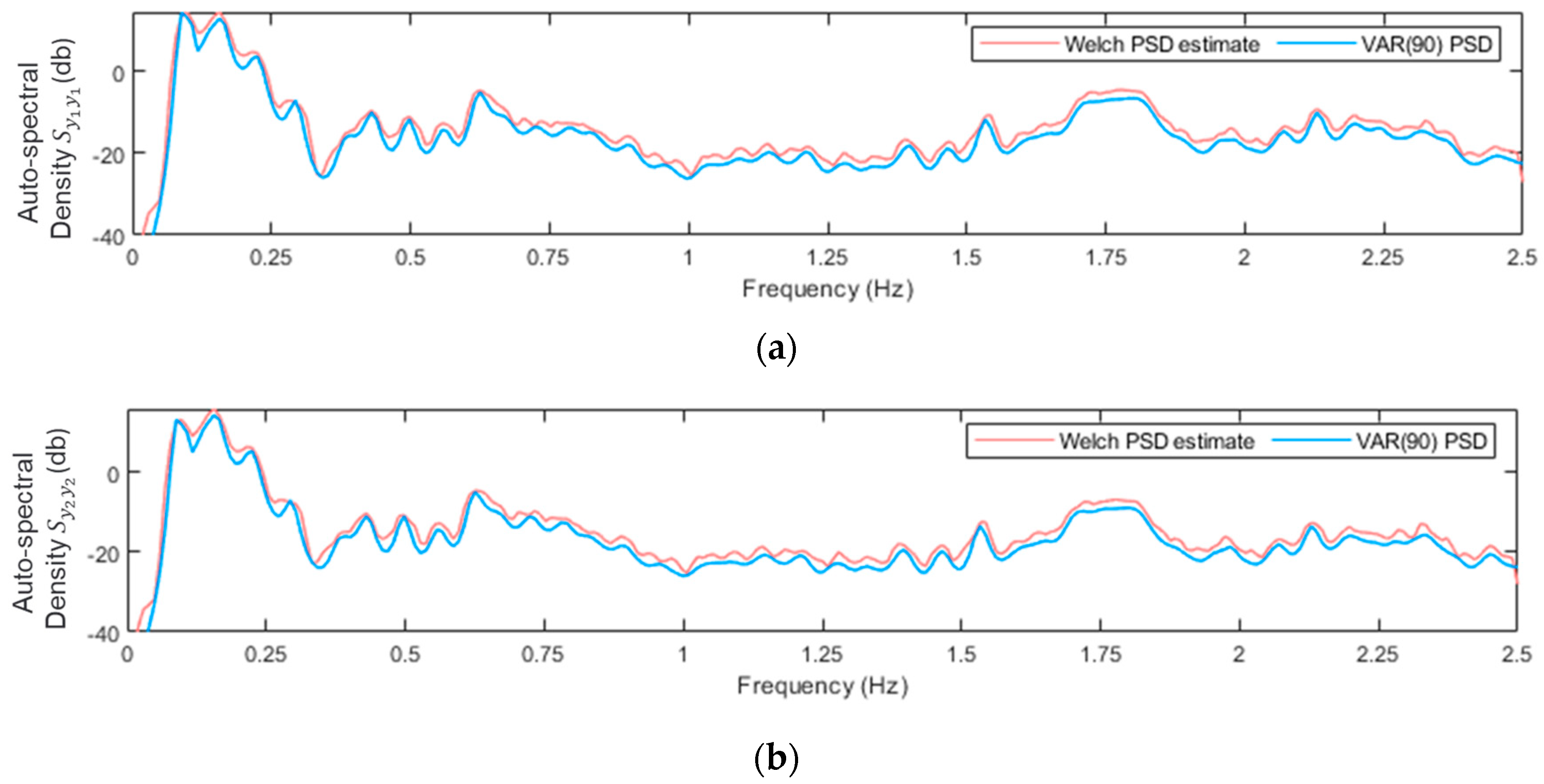
In the MM-based methods, the primary goal is to determine the most suitable orders for the VAR and TF-ARX models. To achieve this, several criteria are considered, including the Akaike information Criterion (AIC), the Bayesian Information Criterion (BIC) and the model-based PSD or TF convergence to their non-parametric (Welch based) counterparts [50]. These criteria are tested for several cases corresponding to different U ¯ h u b . For the VAR models, a good approximation of the structural dynamics is given with order n a = 90 . The adequacy of this order is demonstrated in Figure 11, where the model’s PSD is compared to its non-parametric estimate for a healthy case with U ¯ h u b = 10 m/s.
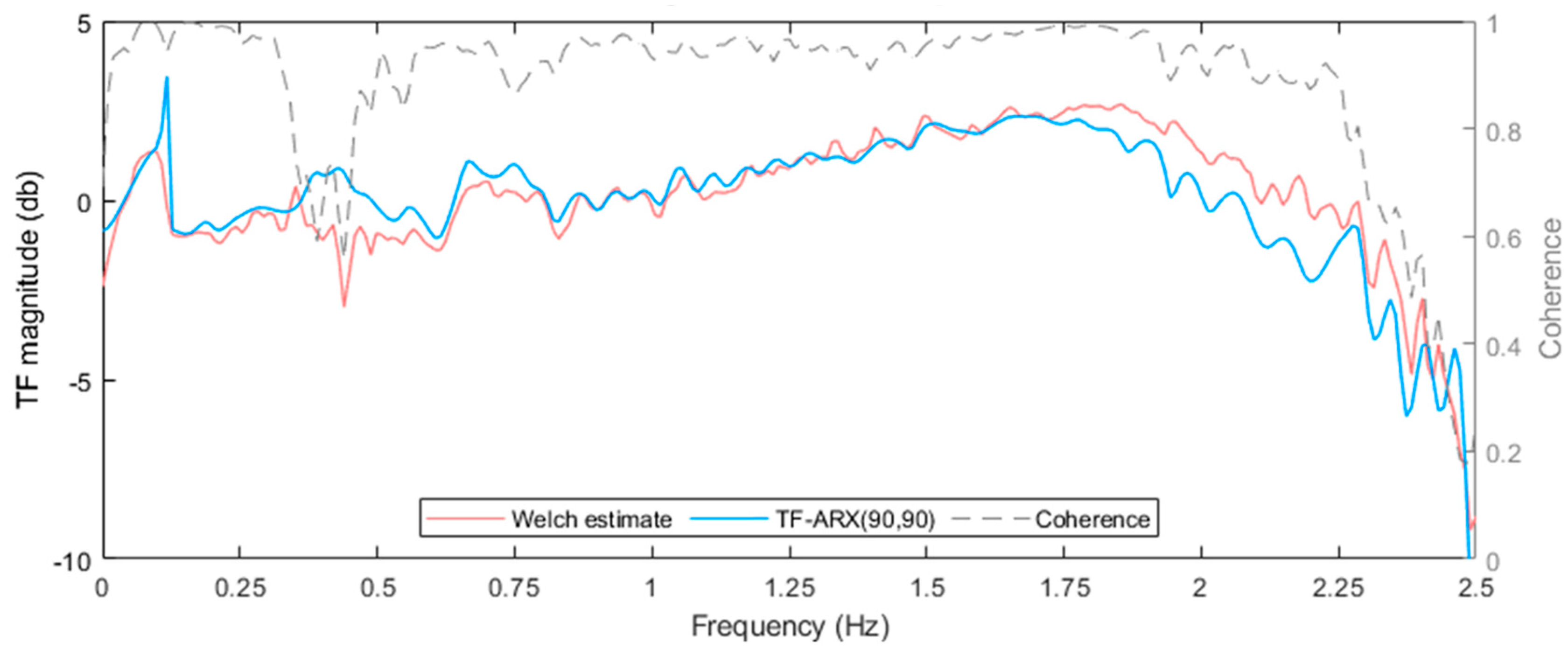
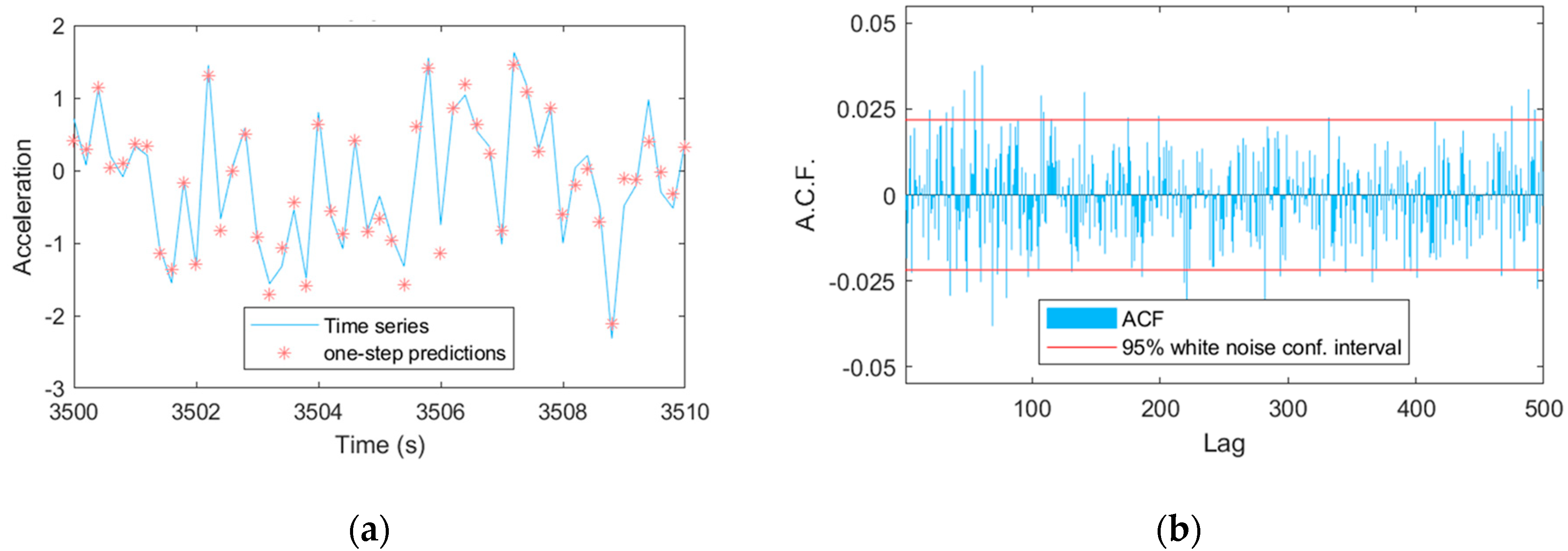
During the TF-ARX identification, notable discrepancies between the models’ and the non-parametric estimates of the TF are observed even for high model orders. These discrepancies are located mainly within the frequency ranges of [0.5 – 0.6] Hz and [1.7 – 2.5] Hz and can be associated with the low coherence function, see in Figure 12. Nevertheless, as with the VAR models, orders n a = n b = 90 are selected for the TF-ARX model based on its accurate one-step prediction, see Figure 13.

4.1.2. PCA-MM Methods

To reduce the parameter subspace dimensionality with the PCA-MM methods, a decrease in variability of γ = 99 % is considered [39], which leads to the selection of 135 components for the TF-ARX models and 314 components for the VAR models, out of their original 181 and 360 parameters, respectively.
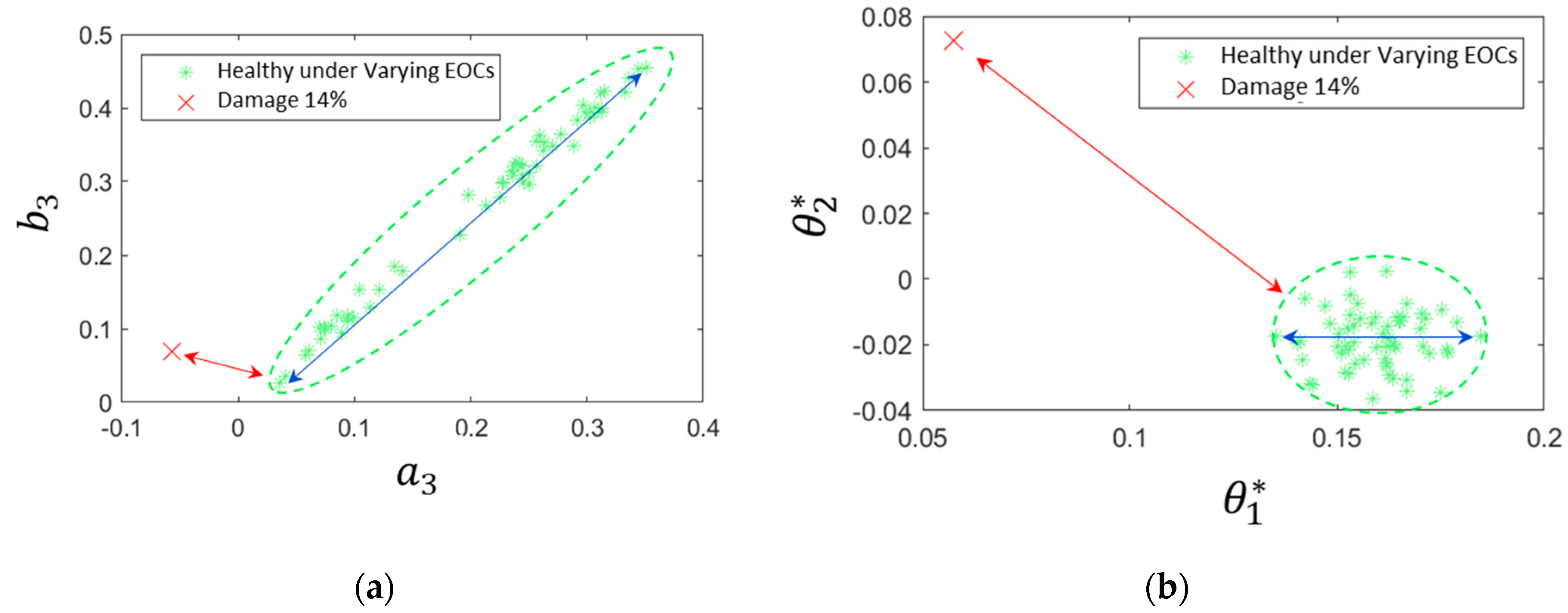
The advantage of the PCA-MM over the simpler MM-based methods is demonstrated in Figure 14. In the figure, two scatter plots are compared, representing each condition with two TF-ARX parameters (see Figure 14a), and with two of the selected principal components (see Figure 14b). The performance of each method depends on the parameters’ or principal components’ sensitivity to damage and to EOCs. In the Figure 14, the sensitivity to damage is represented by the minimum distance between damaged and healthy states (red arrows) while the sensitivity to EOCs is represented by the maximum distance between cases of the healthy state (blue lines). It is shown that in the MM-based method (see Figure 14a), the sensitivity to EOCs (blue arrows) is much higher than the sensitivity to damage (red line), while the opposite holds true for the PCA-MM method (see Figure 14b).

4.1.3. FM Based Method

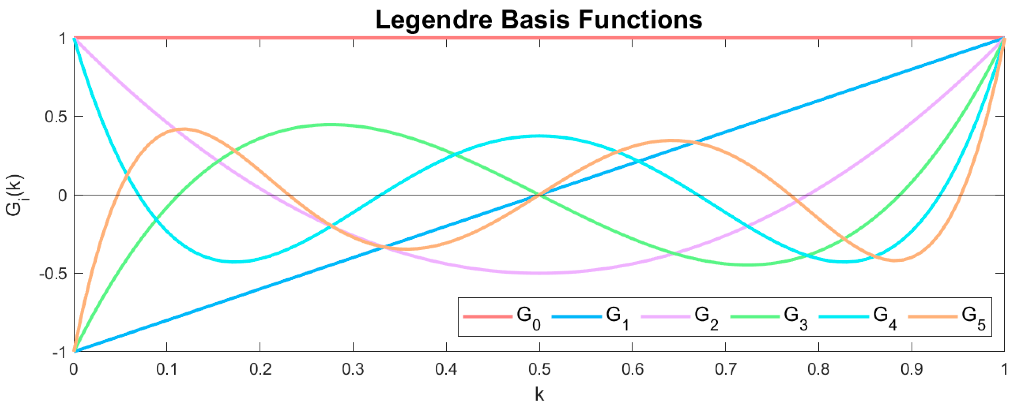
The FP model structure identification based on the baseline dataset Z M N involves the n a and n b orders determination, as well as the selection of the appropriate basis function type and dimensionality [40,44,45]. To simplify the identification problem, the decision is made to employ the same orders as those used for the corresponding VAR and TF-ARX models. For the basis functions, Legendre polynomials of one variable are employed, where each function G i k corresponds to a distinct polynomial order, see Figure 15. The number and combination of Legendre polynomial orders is determined by minimizing the BIC criterion tested for different combinations. The resulting structures for the FP-VAR and FP-TF-ARX models are presented in Table 3.

4.2. Inspection Phase

To evaluate the six methods, detection results are obtained for cases representing known healthy and damaged states, where the damage states involve a 10% and 14% reduction in a mooring line stiffness. For each state, 11 scenarios of varying EOCs are considered (refer to Table 1), and for each scenario, ten cases are employed, with each case corresponding to a simulation using a different random seed. It is worth emphasizing that cases with U ¯ h u b not included in the baseline dataset are tested in the inspection phase as well.
As described in section 3.2, a decision about damage occurrence is determined when the methods’ metrics exceed certain critical thresholds. In the case of MM-based and PCA-MM based methods, where the metric is the minimum Mahalanobis distance δ θ ^ m i n or δ θ ^ m i n * (see equations (25-27)), the critical limit l l i m is user selected in the baseline phase. For the FM-based methods, the threshold may be set according to the statistical critical value of the portmanteau test metric, or alternatively via a user selected value. The latter option is adopted in this study and a user selected critical limit is employed, which is determined as the mean value of the metric plus three standard deviations using the signals of the healthy cases in the baseline phase.
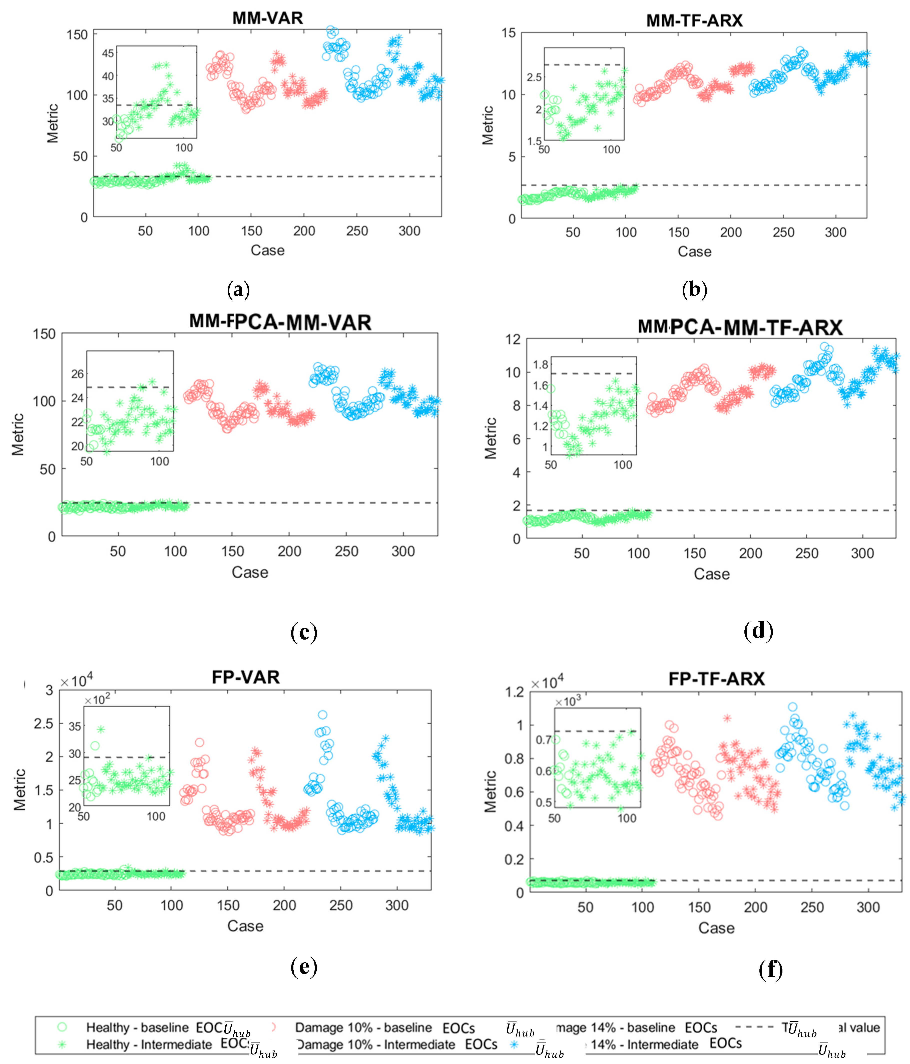
The damage detection results are illustrated through scatter plots in Figure 16. Each subfigure in the figure corresponds to one of the six employed methods. Within the subfigures, the inspection cases which have similar U ¯ h u b values (7 m/s, 8 m/s,….,12 m/s) to the ones used in the baseline phase (see Table 1) are symbolized with circle and they are distinguished from the cases with intermediate U ¯ h u b values (7.4 m/s, 8.6 m/s,….,11.4 m/s) and they are symbolized with asterisk. Table 4 shows the detection results in terms of false alarms and correct detections for the model of each method. False alarms refer to instances where known healthy cases are inaccurately categorized as damaged. Within the table, false alarms corresponding to U ¯ h u b value not encountered in the baseline phase are also shown separately.

5. Discussion

From the results shown in Figure 16 and Table 4, it is indicated that all six method are able to detect damage in the synthetic mooring lines with 100% detectability. A significant rate of false alarms is obtained from the MM-VAR method, see Figure 16a. As shown in Figure 16a, most of these false alarms correspond to cases based on U ¯ h u b values intermediate to the baseline U ¯ h u b values. When employing the PCA-MM-VAR (see Figure 16c) and FP-VAR based methods (see Figure 16e), the false alarm rate drops significantly, aligning with the intended objective of these methods. Methods MM-TF-ARX (see Figure 16b), PCA-MM-TF-ARX (see Figure 16d) and FP-TF-ARX (see Figure 16f) exhibit excellent results, with zero false alarms.
Based solely on these results, neither the FM nor the PCA-MM based methods seem to have an advantage over the other. However, it’s important to note that the performance of the PCA-MM method, may depend on the selection of the variability reduction γ , which is arbitrary in the absent of damaged-state data in the baseline phase, as discussed in section 3.1.2.
The above results pertain to the methods implementation using measuring positions 11-10 and 9-10 in the x direction, which were selected in Section 2.6 for the VAR and TF-ARX-based methods’ variations respectively. To assess their sensitivity, the methods are also employed using positions with a suboptimal ranking based on the F R A C , F A A C and L A C ¯ criteria. In particular, measurements from positions 5-6 (see Figure 3b) in the x direction are tested. Based on the results shown in Table 5, the methods perform equally well with these measuring positions, in comparison with the results of positions 11-10 and 9-10. This is a significant advantage from a practical point of view, as these positions are located at depths less than 30 m, making sensor installation significantly easier compared to sensor pair 10 and 9, located at depth close to 80 m.
Finally, as depicted in all subfigures of Figure 16, there is a clear 'separation' between the healthy and damaged states. This implies that defining a critical limit capable of yielding optimal results for any method is feasible, although data from damaged states would be necessary for such determinations.

6. Conclusions

The problem of damage detection in FOWT synthetic mooring lines under varying environmental and operational conditions using robust vibration-based SHM methods has been investigated for the first time in this study. Six methods were employed based on either Vector (multivariate) AutoRegressive (VAR) or on scalar Transmittance Function AutoRegressive with eXogenous (TF-ARX) data-driven multiple and functional models. The PCA variants of the multiple model-based methods were also explored. All methods evaluation was achieved based on 390 Monte-Carlo simulations via the finite element model of the 10MW FOWT supported by the OO-Star Wind Floater and the main conclusions follow:
  • Both PCA-MM based methods and FM based methods reduce the false alarm rate associated to the simpler MM based methods.
  • The methods utilizing TF-ARX models outperform those using VAR models achieving perfect detection with zero false alarms.
  • The above methods present excellent results even if sensors at randomly selected positions on the mooring line are used. This facilitates robust SHM as sensors at relatively shallow depths with simple installation may be employed.
Overall, the results of the current proof-of-concept study indicate that the explored robust SHM methods are a viable solution for the remote condition monitoring of synthetic mooring lines in FOWTs.
Future plans include the investigation of additional types and magnitudes of early-stage damages in synthetic mooring lines under varying environmental and operational conditions, in order to explore the methods limits, as well as the methods assessment using experimental data which due to actual operating FOWTs recency, data from synthetic mooring lines is not yet available, especially under damage conditions.

Author Contributions

Conceptualization, Nikolas Anastasiadis, Christos Sakaris.; methodology, Nikolas Anastasiadis, Christos Sakaris; software, Nikolas Anastasiadis; validation, Nikolas Anastasiadis; formal analysis, Nikolas Anastasiadis; investigation, Nikolas Anastasiadis; resources, Rune Schlanbusch; data curation, Christos Sakaris, Rune Schlanbusch; writing—original draft preparation, Nikolas Anastasiadis, Christos Sakaris; writing—review and editing, Nikolas Anastasiadis, Christos Sakaris, Rune Schlanbusch, John S. Sakelariou; visualization, Christos Sakaris, Rune Schlanbusch; supervision, Christos Sakaris, Rune Schlanbusch; project administration, Rune Schlanbusch; funding acquisition, Rune Schlanbusch. All authors have read and agreed to the published version of the manuscript.

Funding

This research work has been funded by the Research Council of Norway (RCN) through the project ”Analytics for asset Integrity Management of Windfarms (AIMWind)”, a collaboration between University of Agder, Norwegian Research Center-NORCE AS and Technical University Delft, grant no. 312486.

Acknowledgments

This research work has been funded by the Research Council of Norway (RCN) through the project ”Analytics for asset Integrity Management of Windfarms (AIMWind)”, a collaboration between University of Agder, Norwegian Research Center-NORCE AS and Technical University Delft, grant no. 312486. Origo Solutions is included as advisory partner. Access to the design of the OO-STAR wind floater has been granted by it’s current owner Bouygues Travaux Publics. The development of the FEM of the OO-STAR floater based FOWT has been funded by the RCN though the project “Fibre Rope Mooring”, grant. no 296732. The simulations have been produced by Tor A. Nygaard and Murat Tutkun of the Institute for Energy and Technology (IFE).

Conflicts of Interest

The authors declare no conflict of interest.

References

  1. European Commission Member States Agree New Ambition for Expanding Offshore Renewable Energy. Available online: https://energy.ec.europa.eu/news/member-states-agree-new-ambition-expanding-offshore-renewable-energy-2023-01-19_en (accessed on 25 August 2023).
  2. U.S. Department of Energy Offshore Wind Market Report: 2023 Edition; 2023;
  3. Global Wind Energy Council Global Wind Report 2023; 2023;
  4. Frohböse, P. Offshore Wind 2023: New Ambitions! New Challenges? Available online: https://www.dnv.com/article/offshore-wind-2023-new-ambitions-new-challenges--243462# (accessed on 25 August 2023).
  5. Rinaldi, G.; Garcia-Teruel, A.; Jeffrey, H.; Thies, P.R.; Johanning, L. Incorporating Stochastic Operation and Maintenance Models into the Techno-Economic Analysis of Floating Offshore Wind Farms. Applied Energy 2021, 301, 117420. [CrossRef]
  6. Shafiee, M.; Brennan, F.; Espinosa, I.A. A Parametric Whole Life Cost Model for Offshore Wind Farms. International Journal of Life Cycle Assessment 2016, 21, 961–975. [CrossRef]
  7. Ren, Z.; Verma, A.S.; Li, Y.; Teuwen, J.J.E.; Jiang, Z. Offshore Wind Turbine Operations and Maintenance: A State-of-the-Art Review. Renewable and Sustainable Energy Reviews 2021, 144, 110886. [CrossRef]
  8. Equinor Hywind Tampen Available online: https://www.equinor.com/energy/hywind-tampen (accessed on 30 August 2023).
  9. Ciang, C.C.; Lee, J.R.; Bang, H.J. Structural Health Monitoring for a Wind Turbine System: A Review of Damage Detection Methods. Measurment Science and Technology 2008, 19. [CrossRef]
  10. Li, H.; Díaz, H.; Guedes Soares, C. A Failure Analysis of Floating Offshore Wind Turbines Using AHP-FMEA Methodology. Ocean Engineering 2021, 234. [CrossRef]
  11. Bae, Y.H.; Kim, M.H.; Kim, H.C. Performance Changes of a Floating Offshore Wind Turbine with Broken Mooring Line. Renewable Energy 2017, 101, 364–375. [CrossRef]
  12. Chaplin, C.; Del Vecchio, C. Appraisal of Lightweight Moorings for Deep Water. 24th Annual OTC 1992. [CrossRef]
  13. Nordgård-Hansen, E.; Schlanbusch, R. Condition Monitoring and Maintenance for Fibre Rope Moorings in Offshore Wind WP7 FIRM (Fiber Rope Mooring); 2022;
  14. Deraemaeker, A.; Worden, K. New Trends in Vibration Based Structural Health Monitoring; Springer, 2010; Vol. 520; ISBN 978-3-7091-0398-2.
  15. Oland, E.; Schlanbusch, R.; Falconer, S. Condition Monitoring Technologies for Synthetic Fiber Ropes - a Review. International Journal of Prognostics and Health Management 2017, 8. [CrossRef]
  16. Gorostidi, N.; Nava, V.; Aristondo, A.; Pardo, D. Predictive Maintenance of Floating Offshore Wind Turbine Mooring Lines Using Deep Neural Networks. Journal of Physics: Conference Series 2022, 2257. [CrossRef]
  17. Jamalkia, A.; Ettefagh, M.M.; Mojtahedi, A. Damage Detection of TLP and Spar Floating Wind Turbine Using Dynamic Response of the Structure. Ocean Engineering 2016, 125. [CrossRef]
  18. Dehkharghani, P.H.; Mir, &; Ettefagh, M.; Hassannejad, R. Mooring Damage Identification of Floating Wind Turbine Using a Non-Probabilistic Approach Under Different Environmental Conditions. Journal of Marine Science and Application 2021, 20, 156–169. [CrossRef]
  19. Liu, Y.; Ferrari, R.; Wu, P.; Jiang, X.; Li, S.; Wingerden, J.-W. van Fault Diagnosis of the 10MW Floating Offshore Wind Turbine Benchmark: A Mixed Model and Signal-Based Approach. Renewable Energy 2021, 164. [CrossRef]
  20. Fassois, S.D.; Sakellariou, J.S. Statistical Time Series Methods for SHM. In Encyclopedia of Structural Health Monitoring; 2009 ISBN 9780470061626.
  21. Zhang, C.; Mousavi, A.A.; Masri, S.F.; Gholipour, G.; Yan, K.; Li, X. Vibration Feature Extraction Using Signal Processing Techniques for Structural Health Monitoring: A Review. Mechanical Systems and Signal Processing 2022, 177. [CrossRef]
  22. Ljung, L. System Identification: Theory for the User; Kailath, T., Ed.; 2nd ed.; PTR PrenticeHall, 1987;
  23. Poulimenos, A.G.; Sakellariou, J.S. A Transmittance-Based Methodology for Damage Detection under Uncertainty: An Application to a Set of Composite Beams with Manufacturing Variability Subject to Impact Damage and Varying Operating Conditions. Structural Health Monitoring 2019, 18, 318–333. [CrossRef]
  24. Kopsaftopoulos, F.; Apostolellis, P.; Fassois, S. Output-Only Parametric Identification of a Scale Cable-Stayed Bridge Structure: A Comparison of Vector AR and Stochastic Subspace Methods. In Proceedings of the 4th International Operational Modal Analysis Conference (IOMAC); 2011.
  25. Kopsaftopoulos, F.; Fassois, S. Scalar and Vector Time Series Methods for Vibration Based Damage Diagnosis in a Scale Aircraft Skeleton Structure. Journal of Theoretical and Applied Mechanics 2011, 49, 727–756.
  26. Entezami, A.; Mariani, S.; Shariatmadar, H. Damage Detection in Largely Unobserved Structures under Varying Environmental Conditions: An AutoRegressive Spectrum and Multi-Level Machine Learning Methodology. Sensors 2022, 22. [CrossRef]
  27. Panagiotopoulos, A.; Dmitri, T.; Spilios, F.D. Damage Detection on the Blade of an Operating Wind Turbine via a Single Vibration Sensor and Statistical Time Series Methods: Exploring the Performance Limits of Robust Methods. Structura Health Monitoring 2022, 22, 433–448. [CrossRef]
  28. Vamvoudakis-Stefanou, K.J.; Sakellariou, J.S.; Fassois, S.D. Vibration-Based Damage Detection for a Population of Nominally Identical Structures: Unsupervised Multiple Model (MM) Statistical Time Series Type Methods. Mechanical Systems and Signal Processing 2018, 111, 149–171. [CrossRef]
  29. Sakaris, C.S.; Sakellariou, J.S.; Fassois, S.D. Random-Vibration-Based Damage Detection and Precise Localization on a Lab–Scale Aircraft Stabilizer Structure via the Generalized Functional Model Based Method. Structural Health Monitoring 2017, 16, 594–610. [CrossRef]
  30. Aravanis, T.-C.; Sakellariou, J.; Fassois, S. On the Functional Model–Based Method for Vibration-Based Robust Damage Detection: Versions and Experimental Assessment. Structural Health Monitoring 2021, 20, 456–474. [CrossRef]
  31. Sakaris, C.; Schlanbusch, R.; Nygaard, T.; Sakellariou, J. Statistical Times Series Based Damage Detection in the Fiber Rope Mooring Lines of the Semi-Submersible OO-STAR Wind Floater. In Proceedings of the 62nd IEEE Conference on Decision and Control (CDC); Marina Bay Sands, Singapore, 2023.
  32. Bak, C.; Zahle, F.; Bitsche, R.; Kim, T.; Yde, A.; Henriksen, L.C.; Hansen Morten, H.; Blasques, J.P.A.A.; Gaunaa, M.; Natarajan, A. The DTU 10-MW Reference Wind Turbine.; 2023;
  33. Yu, W.; Müller, K.; Lemmer, F. LIFES50+D4.2: Public Definition of the Two LIFES50+ 10MW Floater Concepts; 2018;
  34. Andersen Oo, H.S.; Eirik, D.; Straume, J.G.; Madsen, M.H.; Laukeland, L.; Landbø, T. Flagship D1.2: Concept Description Report; 2021;
  35. Borisade, F.; Bhat Jayesh; Matha Denis LIFES50+D5.5: Overall Summary of the Industrialization Process; 2019;
  36. Matha, D.; Brons-Illig, C.; Mitzlaff, A.; Scheffler, R. Fabrication and Installation Constraints for Floating Wind and Implications on Current Infrastructure and Design. Energy Procedia 2017, 137, 299–306. [CrossRef]
  37. Pegalajar-Jurado, A.; Bredmose, H.; Borg, M.; Straume, J.G.; Landbø, T.; Andersen, H.S.; Yu, W.; Müller, K.; Lemmer, F. State-of-the-Art Model for the LIFES50+ OO-Star Wind Floater Semi 10MW Floating Wind Turbine. Journal of Physics: Conference Series 2018, 1104. [CrossRef]
  38. Nygaard, T.A.; De Vaal, J.; Pierella, F.; Oggiano, L.; Stenbro, R. Development, Verification and Validation of 3DFloat; Aero-Servo-Hydro-Elastic Computations of Offshore Structures. Energy Procedia 2016, 94, 425–433. [CrossRef]
  39. Jonkman, J.M.; Kilcher, L., TurbSim user’s guide: Version 1.06.00. National Renewable Energy Laboratory, U.S. Department of Energy Office of Energy Efficiency & Renewable Energy, Tech. Rep. NREL/TP-xxx-xxxx, 2012.
  40. Chakrabarti, S. Handbook of Offshore Engineering; Elsevier, 2005; ISBN 0080523811.
  41. Bendat, J.S.; Piersol, A.G. Random Data: Analysis and Measurement Procedures; John Wiley & Sons, 2011; ISBN 1118210824.
  42. Sakellariou, J.S.; Fassois, S. A Functional Pooling Framework for the Identification of Systems under Multiple Operating Conditions. In Proceedings of the 2007 Mediterranean Conference on Control & Automation; July 29 2007; pp. 1–6.
  43. Sakellariou, J.S.; Fassois, S.D. Functionally Pooled Models for the Global Identification of Stochastic Systems under Different Pseudo-Static Operating Conditions. Mechanical Systems and Signal Processing 2016, 72–73, 785–807. [CrossRef]
  44. Hios, J.D.; Fassois, S.D. Stochastic Identification Under Multiple Operating Conditions: Functionally Pooled VARMA Methods. IFAC Proceedings Volumes 2009, 15, 1626–1631. [CrossRef]
  45. Lutkepohl, H. New Introduction to Multiple Time Series Analysis; 2nd ed.; Springer, 2005; ISBN 9783540277521.
  46. Ljung, L. System Identification: Theory for the User; Kailath, T., Ed.; 2nd ed.; PTR PrenticeHall, 1987;
  47. Gómez González, A.; Fassois, S.D. A Supervised Vibration-Based Statistical Methodology for Damage Detection under Varying Environmental Conditions & Its Laboratory Assessment with a Scale Wind Turbine Blade. Journal of Sound and Vibration 2016, 366, 484–500. [CrossRef]
  48. Mosavi, A.A.; Dickey, D.; Seracino, R.; Rizkalla, S. Identifying Damage Locations under Ambient Vibrations Utilizing Vector Autoregressive Models and Mahalanobis Distances. Mechanical Systems and Signal Processing 2012, 26, 254–267. [CrossRef]
  49. Ljung, G.M.; Box, G.E.P. On a Measure of Lack of Fit in Time Series Models. Biometrika 1978, 65, 297–303. [CrossRef]
  50. Fassois, S.D. Identification, Model-Based Methods. In Encyclopedia of Vibration; Braun, S., Ed.; Elsevier: Oxford, 2001; pp. 673–685 ISBN 978-0-12-227085-7.
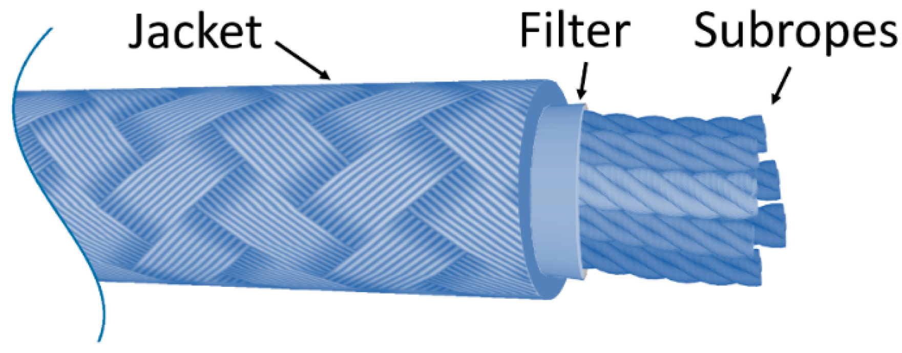
Figure 1. Parallel sub-rope mooring line composition.
Preprints 91074 g001
Figure 2. Mooring line segment’s modelling based on the TF of two acceleration signals. Preprints 91074 i001 : accelerometer measuring position.
Preprints 91074 g002
Figure 3. (a) The OO-Star Floater based 10MW FOWT and (b) the measuring positions on the synthetic fiber rope and the floater.
Preprints 91074 g003
Figure 4. Welch-based estimates of the PSDs of acceleration signals corresponding to measuring position 11 in the x direction, under varying U ¯ h u b   7 ,   12 m/s and corresponding H s , T p (refer to Table 2), for healthy and damaged states: (a) damage level 10%; (b) damage level 14%. For the Welch estimate: Hamming Window; window size: 350; f s   = 5 Hz; overlap: 95%; sample size N = 8500 .
Preprints 91074 g004
Figure 5. Welch-based coherence function of acceleration signals in the x direction corresponding to measuring positions: (a) 5-6; (b) 9-10; (c) 10-11 and (d)12-13. For the Welch estimate: Hamming Window; window size: 350; f s   = 5 Hz; overlap: 95%; Sample size N = 8500 . Shown for case under U ¯ h u b = 10 m/s.
Preprints 91074 g005
Figure 6. Welch-based TF of acceleration signals corresponding to measuring positions 10 and 9 in the x direction under U ¯ h u b   7 ,   12 m/s and corresponding H s , T p (refer to Table 2), in the healthy and damaged states: (a) damage level 10%; (b) damage level 14%. For the Welch estimate: Hamming Window; window size: 350; f s   = 5 Hz; sample size N = 8500 ; overlap: 95%.
Preprints 91074 g006
Figure 7. (a) Welch-based PSD of acceleration signals corresponding to measuring position 11 in the x direction and (b) Welch-based TF of acceleration signals corresponding to at positions 10 and 9 in the x direction for realizations with different random seeds under U ¯ h u b = 10 m/s. For the Welch estimate: Hamming Window; window size: 350; f s   = 5 Hz; sample size N = 8500 ; overlap: 95%.
Preprints 91074 g007
Figure 8. F A A C , F R A C and L A C ¯ criteria for different measuring positions and based on: (a) PSD and (b) TFwith acceleration signals in the x direction.
Preprints 91074 g008
Figure 9. Representation of the structural dynamics: (a) discrete subspace representation based on MM; (b) subspace dimensionality reduction using PCA; (c) continues subspace representation based on a FP model.
Preprints 91074 g009
Figure 10. Damage detection framework: (a) baseline phase process diagram; (b) inspection phase process diagram.
Preprints 91074 g010
Figure 11. VAR(90) model-based PSD, and non-parametric PSD Welch estimate: (a) Auto-spectral density S y 1 y 1 ; (b) Auto-spectral density S y 2 y 2 . For the Welch estimate: Hamming Window; window size: 350; f s   = 5 Hz; sample size N = 8500 ; overlap: 95%. Shown for case under U ¯ h u b = 10 m/s.
Preprints 91074 g011
Figure 12. TF-ARX(90,90) model-based TF, Welch based TF and coherence Welch estimates. For the Welch estimates: Hamming Window; window size: 350; f s   = 5 Hz; sample size N = 8500 ; overlap: 95%. Shown for case under U ¯ h u b = 10 m/s.
Preprints 91074 g012
Figure 13. TF-ARX(90,90) model validation: (a) one-step predictions and (b) residual signals’ Autocorrelation Function (ACF). Shown for healthy case under U ¯ h u b = 10 m/s.
Preprints 91074 g013
Figure 14. (a) TF-ARX parameter scatter plot for healthy and damaged conditions; (b) TF-ARX PCA component scatter plot for healthy and damaged conditions. Blue arrows: the maximum distance among all healthy cases of the baseline phase; Red arrows: the minimum distance between a damaged case and all healthy cases of the baseline phase.
Preprints 91074 g014
Figure 15. First five Legendre orthogonal polynomials.
Preprints 91074 g015
Figure 16. Damage detection results based on the method variations: (a) MM-VAR; (b) MM-TF-ARX; (c) PCAMM-VAR; (d) PCA-MM-TF-ARX; (e) FM-VAR; (f) FM-TF-ARX. Critical values correspond to three standard deviations from the healthy-baseline   U ¯ h u b based metric distributions. Results of (a),(c) and (e) correspond to measuring positions 10-11 and (b),(d) and (f) to 9-10.
Preprints 91074 g016
Table 1. Baseline and Inspection phase scenarios (structural state and wind speed) and data description.
Structural State Mean wind speed
(m/s)
No. of simulations per scenario Total no. of
simulations
(set of acceleration signals)
Baseline Phase Healthy 7,8,9,10,11,12 10 60
Inspection Phase Healthy,
Mooring line stiffness reduction: 10%, 14%
7, 7.4, 8, 8.6, 9, 9.5, 10, 10.7, 11, 11.4, 12, 10 330
Sampling frequency: f s = 5 H z , Signal Bandwidth: 0 2.5 H z , Signal Length: N = 8500 samples.
Table 2. The considered mean wind speeds at hub height U ¯ h u b and the corresponding significant wave height H s and peak periods T p .
U ¯ h u b (m/s) 7 7.4 8 8.6 9 9.5 10 10.7 11 11.4 12
H s (m) 1.89 1.95 2.04 2.14 2.21 2.30 2.39 2.53 2.59 2.68 2.81
T p (s) 9.02 9.06 9.13 9.20 9.26 9.32 9.39 9.49 9.54 9.60 9.70
Table 3. FP-VAR and FP-TF-ARX model structure identification results.
Model type Orders Basis function type Number of selected basis functions Polynomial orders Number of projection coefficients Samples per projection coefficient
FP-VAR n a = 90 Legendre polynomials p = 5 0,1 , 2,3 , 4 1800 566.6
FP-TF-ARX n a = 90 , n b = 90 p = 4 0,1 , 2,3 724 1408.9
Table 4. Damage detection results overview.
VAR/ FP-VAR
Measuring positions
11 – 10 for x direction
False Alarms Correct Detections
Method Similar to
baseline U ¯ h u b
Intermediate to
baseline U ¯ h u b
Total 10% Stiffness
reduction
14% Stiffness
reduction
MM-VAR 1/60 17/50 18/110 110/110 110/110
PCA-MM-VAR 0/60 2/50 2/110 110/110 110/110
FM-VAR 1/60 1/50 2/110 110/110 110/110
TF-ARX/ FP-TF-ARX
Measuring positions
10 -9 for x direction
False Alarms Correct Detections
Method Similar to
baseline U ¯ h u b
Intermediate to
baseline U ¯ h u b
Total 10% Stiffness
reduction
14% Stiffness
reduction
MM-TF-ARX 0/60 0/50 0/110 110/110 110/110
PCA-MM-TF-ARX 0/60 0/50 0/110 110/110 110/110
FM-TF-ARX 0/60 0/50 0/110 110/110 110/110
Table 5. Damage detection results employing acceleration signals from measuring position 5 and 6 in the x direction.
VAR/ FP-VAR
Measuring positions6 – 5 for x
direction
False Alarms Correct Detections
Method Variation Similar to
baseline U ¯ h u b
Intermediate to
baseline U ¯ h u b
Total 10% Stiffness
reduction
14% Stiffness
reduction
MM-VAR 0/60 18/50 18/110 110/110 110/110
PCA-MM-VAR 0/60 3/50 3/110 110/110 110/110
FM-VAR 0/60 1/50 1/110 110/110 110/110
TF-ARX/ FP-TF-ARX
Measuring positions
6- 5 for x direction
False Alarms Correct Detections
Method Variation Similar to
baseline U ¯ h u b
Intermediate to
baseline U ¯ h u b
Total 10% Stiffness
reduction
14% Stiffness
reduction
MM-TF-ARX 0/60 0/50 0/110 110/110 110/110
PCA-MM-TF-ARX 0/60 0/50 0/110 110/110 110/110
FM-TF-ARX 0/60 0/50 0/110 110/110 110/110
Disclaimer/Publisher’s Note: The statements, opinions and data contained in all publications are solely those of the individual author(s) and contributor(s) and not of MDPI and/or the editor(s). MDPI and/or the editor(s) disclaim responsibility for any injury to people or property resulting from any ideas, methods, instructions or products referred to in the content.
Copyright: This open access article is published under a Creative Commons CC BY 4.0 license, which permit the free download, distribution, and reuse, provided that the author and preprint are cited in any reuse.
Prerpints.org logo

Preprints.org is a free preprint server supported by MDPI in Basel, Switzerland.

Subscribe

© 2024 MDPI (Basel, Switzerland) unless otherwise stated