
Submitted:
16 November 2023
Posted:
21 November 2023
You are already at the latest version
Abstract
Availability and continuous operation under critical conditions are very important in electric machine drive systems. However, such systems, are suffering from several type of failures that affect the electric machine or the associated voltage source inverter. Therefore, fault diagnosis and fault tolerance are highly required. This paper presents a new robust deep learning-based approach to diagnosis multiple open-circuit fault in three phase two level voltage source inverter for induction motor drive applications. The proposed approach uses fault diagnosis variables obtained from sigmoid transformation of the motor stator currents. The open-circuit fault diagnosis variables are then introduced to a Bidirectional Long Short-Term Memory algorithm to detect the faulty switch(es). Several simulation and experimental results are presented to show the proposed fault diagnosis algorithm effectiveness and robustness.
Keywords:
Fault Diagnosis
; Power Converters
; Open-Circuit Fault
; Deep Learning
; AC drives
1. Introduction
Three phase pulse width modulated (PWM) voltage source inverters (VSI) have been widely used for grid connected converters or AC machines variable speed drives applications. For the most of these applications, high reliability and high availability are of utmost importance. Consequently, condition monitoring, fault detection and fault tolerant control of thee phase PWM VSIs are mandatory functions that should be added to the drive system’s controller [1,2].
Open-circuit fault is one of the most relevant faults that may affect induction motor speed variable drives [3]. This type of fault may affect multiple power semi-conductors. As discussed in [3,4], it introduces severe perturbations with a DC current injection and high oscillations of the electromagnetic torque and, in some cases, the electric drive must be shut down. Hence, it is important to diagnosis such type of fault. Open-circuit (OC) fault diagnosis issue has been discussed in several studies and different methods have been proposed [5,6,7,8]. They are generally classified as Model-based approaches [9,10,11,12,13,14,15,16,17,18,19,20,21] and signal-based approaches [26,27,28,29,30].
Model-based fault diagnosis approaches, use the mathematical model of the electric machine and/or the model of the voltage source inverter. The main idea is to compare some estimated quantities obtained from the system’s model to the measured quantities. In most cases, electric machine currents [9,10,11,12,13,14] and voltage source inverter output voltages [15,16,17,18,19,20] are the estimated quantities.
In healthy operation, measured and estimated quantities are almost the same. Hence, the estimation error converges to zero. When an open-circuit fault is affecting one or more power switch(es), the deviation of the estimation error is used to detect the fault and to identify the faulty switch(es).
In [9,10], Jlassi et al. uses the current form factor (CFF) to detect open-circuit faults in permanent magnet synchronous machine (PMSM) drives for both generator and motor applications. The main idea is to compare the CFF obtained from the measured currents to the CFF obtained from estimated currents based on state Luenberger observer. A similar approach is discussed in [11] to detect currents sensor and open-circuit fault in grid connected three level NPC inverters. In this study, the currents are estimated using a sliding mode observer.
The current residual approach is proposed to diagnosis open-circuit faults in PMSM and induction motor drive systems are discussed in [12] and [13] respectively.
Voltage based OC fault detection, had been discussed in [15,16,17,18,19]. To avoid the use of additional voltage sensors, which may increase the system’s cost, the output voltage of the VSI should be estimated. In [15], an OC fault diagnosis scheme is proposed based on voltage estimation for an induction machine drive system. A state estimator is used to estimate the phase voltage based on the induction machine model. The estimated voltage is compared the voltage obtained from the DC-link voltage and the inverter switching signals. The residual of the estimation error is used to detect the faulty switch(es). Nevertheless, this approach needs the use of low pass filters that need high tuning and introduce delays in the detection time. Freire et al., presents a similar approach applied to PMSM drive systems [16]. In [17], the calculated common mode voltage behavior is used to detect and locate OS faults in three phase two level inverters for induction machine drive system.
Model based OC fault detection approaches had shown their effectiveness, but they need a good knowledge of the studied system’s model, they should be less sensitive to system’s parameters variations. Moreover, they required a robust fault detection threshold which makes them complex to be contructed.
Rencently, with the increase of the use of model predictive control (MPC) in variable speed drive systems, some studies propose to use the motor prediction current errors to detect OC fault for PMSM drive systems [22,23,24,25]. Thanks to the robustness of MPC, the motor current prediction errors are very low in healthy operation mode. It has been shown that in case of OC faults, the motor current prediction errors increase allowing to detect and to identify the fault switch.
Signal based methods are generally based on current analysis [26,27,28,29,30]. In [26], a single current sensor is employed to detect OS faults in PMSM drive system. The DC-link current sensor is used to reconstruct the motor stator currents. Then after, the normalized average value of the reconstructed current is used to detect the faulty switch. Sejir et al. [27], presents a current analysis-based algorithm to detect OS faults in PMSM drive systems. The fault detection variables use the interaction between two stator currents which allow to detect 27 types of OC faults and current sensor faults. Reference current errors are employed to detect OC faults in voltage source inverters [28]. However, this approach can only be used for closed loop controlled electric drives.
More recently, intelligence artificial tools had become more attractive for fault diagnosis and fault classification issues [31,32,33,34,35,36,37,38,39,40,41,42,43]. Indeed, data driven approaches are only based on recorded data obtained from measured quantities instead of specific complex mathematical models.
In [31,32], a Fast Fourrier Transform (FFT) algorithm is used to extract open-circuit fault features from motor current [31] or inverter’s output line-to-line voltage [32]. Then, a fast-learning technology is applied to diagnosis the faulty switch(es). Xia et al. [33] presents a transferrable data driven algorithm for open-circuit switch fault diagnosis in three phase inverters. Deep learning-based approach for open switch fault diagnosis of three phase PWM converters is discussed in [34]. Currents behavior in healthy and faulty operation modes are analyzed for fault features extraction.
Recently, Long Short-Term Memory Network (LSTM) networks have became more and more attractive in fault diagnosis issues due to their high accuracy over other fault diagnosis techniques [36,37,38,39,40,41,42,43]. The effectiveness of the method is confirmed in [36] where it is used to detect multiple open-circuit switch faults of the back-to-back converter in doubly-fed induction generator (DFIG)-based wind turbine systems. Similar approach has been used to diagnosis open-circuit faults in multilevel converters [37,38,39]. LSTM approach is applied for diagnosing faults in Electric Vehicles [40,41] and for motor electrical fault [42] and mecanical fault diagnosis [43].
To deal with the above mentioned issues, this paper proposes a Bidirectional Long Short-Term Memory (BiLSTM) based algorithm to diagnosis open-circuit power semiconductor faults in three phase PWM voltage source inverter for an induction motor drive system. The proposed method is able to achieve accurate diagnosis of single and multiple open-circuit faults without any extra hardware requirements. Only already measured induction motor stator currents are used. To keep the fault diagnosis method free from load torque and motor speed variations, the induction motor stator currents are normalized using the sigmoid function. Then, three fault detection variables are defined and introduced to the BiLSTM network to identify the faulty switch(es). Moreover, the BiLSTM network does not need to set any fault detection threshold which increases the accuracy and the effectiveness of the proposed approach.
The rest of the paper is organized as follows: Section 2 presents the fault detection variables and analysis the fault features. Section 3 describes the BiLSTM network and the fault diagnosis algorithm. The simulation results are presented in Section 4 and the performances of the proposed approach are experimentally analyzed in Section 5. Finally, conculsions are drawn in Section 6.
2. Fault Features Analysis
The structure of the three-phase induction motor drive system is depicted out in Figure 1. The two level VSI is composed of six IGBTs (T1 → T6) and their anti-parallel diodes. Under healthy operation conditions, the induction motor stator currents are expressed as:
where Im is the induction motor stator current amplitude and ɷ is the synchronous electrical pulsation. When an open circuit fault occurs, it produces distortion of the stator currents with the increase of their amplitude, electromagnetic torque oscillation and excess heat which can lead to motor failure [3]. Hence, the motor current measurement can be used to pinpoint open-circuit faults.
Motor current based open-circuit fault methods should be less sensitive to motor paramters mismatch or operating point variations. Therefore, the normalization of the motor current measurement is required. In this way, several approaches have discussed by the literature where the Park Vector’s Modulus in [23], the maximum absolute value of the motor phase currents in [27] and the average absolute values of the motor phase currents in [28] are proposed as normalization tools. Although these methods give good results, they also require additional computational effort and prior knowledge of the motors parameters to ensure a real-time normalization of diagnosis variables which increases computation time and decreases the performance of the OC fault methods.
In this work, the main idea is to apply the sigmoid function to motor currents for the normalization process. The sigmoid function of the real variable x, F(x), is defined as:
where λ is a positive real. In Figure 2, is presented the sigmoid function of the sinusoidal variable x. It can be seen that F(x) vary between ±1 and has the same period as the variable x. The impact of the positive real λ on the dynamic of F(x) is depicted out in Figure 2. More λ is higher more F(x) variation is faster.
where xm is the amplitude of the current signal x(t).
However, the sampled currents are not smooth, which involve the notch due to the PWM and noise due to measurement in the actual current sampling process of the motor drive system. As result, the chattering problem appears in normalized function that it can be seen during the zero crossing of the current signal as shown in Figure 3a. To analyze this feature, take the positive current half period as an exemple: the current can be divided into two zones according to the zero-crossing of current signal. Zone1 is the chattering area since the current drop in this zone is soo small. Zone 2 is the no-chattering area due to enough current drop. Therefore, this problem makes it difficult, if not impossible, to detect occured faults during this time.
To reduce the chattering effect of the sigmoid function, the normalization function of the induction motor stator current is modified and expressed as below:
where xh is the minimum value of signal x(t) that avoid the chattering problem. Figure 3b shows the output of the modified normalization function where it is forced to be zero during the zero-crossing of the current signal. Sowhen , the fault occurring during [t1; t2] can be detected immediately in [t2; t3] by the proposed algorithm, but the fault occurring during [t3; t4] must wait for the second chance for diagnosis in the next cycle.
By applying Equation (3) to the stator currents of the induction motor, we obtain the variations of the sigmoid variables Fa, Fb and Fc of the stator currents ia, ib and ic as presented in Figure 4a. Accordingly, three fault diagnosis indictors χa, χb and χc are defined as:
The variations of the induction motor stator currents, their respective sigmoid functions and the fault diagnosis indicators for one period of the stator currents are depicted out in Figure 4b. The fault detection variables have similar behavior of the motor stator currents with the same period and a phase shift between them equal to 2π/3. Moreover, they vary between ±4. It should be noted that the variations of the fault detection variables are independent from motor speed or load torque.
When an open-switch fault occurs, it affects the stator currents waveforms and then after Fa, Fb and Fc and χa, χb and χc waveforms also. In Figure 5a are described the stator currents and the detection variables χa, χb and χc variations in case of open-switch fault of the IGBT T1 applied at time t=0.6s. Instantly, the behavior of χa, χb and χc is not the same as in healthy operation mode. Indeed, χa lost its positive sequence, whereas χb and χc vary between 4 and -3.
Similar analysis has been done for open-switch fault of T1 and T2 (open phase fault), as presented in Figure 5b. χa becomes equal to 0 and χb and χc are opposite and vary between 3 and -3. A third fault case is analyzed considering an open-switch fault of T1 and T4 depicted out in Figure 5c. In this case, χa lost its positive sequence, χb lost its negative sequence and χc vary between 3 and -3. The analysis of these three fault scenarios has shown for each open-switch fault, the detection variables χa,b,c have a specific feature, which make them suitable to be employed to achieve robust and reliable open-switch fault detection algorithm for the studied electric drive system.
3. LSTM Approach for Fault Diagnosis
3.1. LSTM Structure
LSTM is an improved version of recurrent neural network (RNN), which has achieved satisfactory performance in sequence learning and temporal modeling [36].
LSTM has a special structure, which allow solving the challenge of gradient vanishing or explosion in a simple RNN since it replaces the iterative transformation in RNN with addition in the calculation of hidden state [43]. The structure of an LSTM unit is illustrated in Figure 6.
LSTM mainly consists of three gates: forget gate , input gate and output gate .The forget gate layer determines which information should be forgotten. The equation of the forget gate layer can be expressed as:
where and represent respectively the input at the current time and the output at previous time of the LSTM network. and represent the weight and the bias of the forget gate layer. is the sigmoid function and [ ] represents the concatenate operation.
The input gate layer updates the cell state based on the input at the current time and the output at previous time . The equations of the input gate can be described as:
where and represent respectively the input at time the current time and the output at previous time. and are the weight and the bias of the sigmoid function in the input gate layer. tanh is a hyperbolic tangent function, and are the weight and the bias of the tanh function in the input gate layer.
The output gate layer selects information that should be the next output which depends on the cell state . The equation of the output gate layer can be expressed as equation (8) with and are the weight and the bias of the output gate layer.
The cell state and the output (hidden) state at time step t are described by the following equations:
3.2. Stacked LSTM (MLSTM)
A stacked LSTM is a deep LSTM that consists of multiple LSTM layers where each layer contains multiple memory cells. The input of the first LSTM layer is the sequence data, and the input of other LSTM layers is the hidden state of the previous LSTM layer. Therefore, the Stacked LSTM hidden layers make the model deeper and more accurate. This type of network becomes a powerful method for challenging sequence prediction problems. The structure of Stacked LSTM with n hidden layers is shown as in Figure 7.
3.3. Bidirectional LSTMs (BiLSTM)
The Bidirectional LSTM is a recurrent neural network which combines two LSTMs together. Unlike standard LSTM, the input flows in both directions forward or backward. In fact, this structure allows the networks to have forward layer and backward layer which reverses the direction of the input sequence flow. Applying the LSTM twice makes the prediction results more integrated and leads to improve the accuracy of the model. On the other hand, it should be mentioned that BiLSTM is a much slower model and requires more time for training. The BiLSTM architecture is presented in Figure 8.
3.4. Evaluation Metrics
After building prediction models, there are several metrics can be used to evaluate the performance of models and compare them.
3.4.1. Root Mean Square Error (RMSE)
The Root Mean Square Error (RMSE) are the most commonly used performance measures for prediction tasks. The RMSE can be calculated by using (11).
where and are the prediction and the real output value, and n is number of data.
3.4.2. Mean Absolute Error (MAE)
The MAE is the other criterion used to evaluate the model performance. The MAE is expressed as (12).
3.4.3. Mean Absolute Percentage Error (MPAE)
The MPAE is one of the most common metrics used to measure the prediction accuracy of a model and it is described as (13).
The summation ignores observations where yi = 0. In general, the lower the MAPE value, the more accurate the model is.
The last metric used in this paper to evaluate the performance of the proposed algorithm is the accuracy of the prediction model that is expressed as:
3.5. Diagnostic Network Implementation and Validation
The proposed diagnosis method consists of BiLSTM network with one hidden layer. The BiLSTM-based network is adopted for the fault diagnosis, using the normalized diagnosis variables χa, χb and χc of current sensor signals as input. Firstly, two-phase current signals collected by the sensors installed between the inverter and the motor, respectively. Then, a normalization process is applied to extract suitable features. Finally, the normalized input sensor data [χa χb χc] are put into BiLSTM network.
The output of BiLSTM network is a concatenation of the forward and backward hidden states. The final output of the network contains 6 flags [T1 T2 T3 T4 T5 T6] which represent the healthy or faulty state of each power switch of the inverter that controls the IM. Each flag can take either the value 1 to indicate that the desired power switch is infected, or the value 0 to indicate that the desired switch is healthy. The proposed BILSTM enables to predict and identify 21 open circuit faulty states and one normal state. The structure the fault diagnosis method based on BiLSTM network is illustrated in Figure 9.
To train LSTM Network to work efficiently, the system requires a normal and faulty feature data. For this, we have generated all possible single and multiple open-circuit fault scenarios. Thirty thousand samples are used as training data for each class of default, with a sampling time s. The cost function used in the training process is the Root Mean Square Error (RMSE).
After many trials ranging from 10 to 100 as shown in Figure 10, the size of the hidden layer of BiLSTM network is set as 100 units to make a tradeoff between accuracy and computation time.
The maximum training epoch is set as 1000 to ensure that the error after training is small enough. The BiLSTM model is trained using LSTM Matlab toolbox.
The parameters of the BiLSTM models are summarized in Table 1.
The principal of the proposed BiLSTM-based fault diagnosis method considering the data detailed above is shown in following algorithm.
| Algorithm 1: BiLSTM-based Fault Diagnosis Algorithm |
Step 1: Data set collection.
Step 3: Set BiLSTM model.
Step 5: Return the network model . Step 6: Test model. If the evaluation metrics are not satisfactory, then adjust network parameters and go to Step 3. |
After training, the performance and efficiency of our network were tested in a situation when open-circuit switch fault occurs simultaneously on T5 and T6 at t = 1s. Simulation results are shown in Figure 11a,b.
It can be seen from the Figure 11b that the validation error value varies between -0.05 and 0.05 with a little increase when the fault begins to occur (t=1s), this demonstrates the efficiency of the proposed model in the prediction of default class and the time when it occurs.
4. Simulation Results
The performances of the proposed open-switch fault detection approach are analyzed first through simulations under Matlab/Simulink Software for a variable speed three phase induction motor drive. In this section, the robustness of the proposed method, under speed/load torque variations is studied first. In the second step, the effectiveness of the proposed approach to detect single and multiple open-switch faults is presented.
4.1. Robustness under Operating Point Variations
The performances of the proposed fault diagnosis approach under motor speed and load torque variations are presented in Figure 12 and Figure 13 respectively. In Figure 12 are presented the variations of the stator currents, motor speed, the detection variables and the output of the BiLSTM network (T1→T6 fault flags), when the motor speed varies from 1200 to 1500 rpm at time t = 1s with no load. The detection variables maintain the same behavior during steady state operation as well as during transient state. Finally, all fault flags remain at low levels equal to 0. Figure 13 describes the same variables in case of torque load change from 0N.m to 3 N.m at time t = 1s with motor speed equal to 1000 rpm. Here again, all fault flags remain at 0 value and no false alarm has been triggered.
4.2. Open-Switch Fault Detection
Figure 14 shows the time domain waveforms of the three phase currents for a single fault in the power switch T1, under 4 N.m as load torque and a 800 rpm as rotor speed. When the open-switch fault of IGBT T1 is applied in t = 1 s, the positive half-cycle of the phase current ia is eliminated. Consequently, the diagnostic variable χa lost is positive sequence and becomes varies between the values -4 and 0 whereas the other both diagnostic variables χb and χc makes the values between -3 and 4. As a result, the identification fault flag of T1 increase immediately to 1 after 4 ms of the fault occurrence, corresponding to 10% of the motor currents fundamental period.
The performance of the proposed algorithm regarding the diagnosis of an open-phase fault is depicted in Figure 15. Firstly, a single open-circuit fault in IGBT T1 is introduced at a time t = 1 s, for a speed of 1400 rpm and a load torque equal to 3 N.m. The faulty IGBT is detected when the T1 fault flag switches from 0 to 1 at a time t = 1.003 s, corresponding to an interval of 14% of motor currents fundamental period. When the second fault, in IGBT T2, is added at a time t = 1.5 s, the behavior of the fault diagnostic variables automatically changes. Regarding all diagnostic variables for this kind of situation (open-phase fault), the first diagnostic variable χa becomes equal to 0 and the other diagnostic variables χb and χc takes the values of -3 and 3. Hence, the open-phase fault is detected when both T1 & T2 fault flags changes from 0 to 1, 4 ms after the fault occurrence, which corresponds to 19% of the motor currents fundamental period.
The steady state performance of the proposed IA algorithm for both open-switch fault in the VSI is presented in Figure 16. Firstly, an open-circuit fault in IGBT T1 is applied at a time t = 1 s, under a speed of 1200 rpm and a load of 3 N.m. The faulty IGBT is localized by switching state of the T1 fault flag that changes from 0 to 1 at t = 1.004s, in an interval of 10% of the fundamental period. When the second fault in IGBT T4 is added in time equal to 1.5 s, the first diagnostic variable χa maintain its negative sequence but the second diagnostic variable χb changes its behavior by losing its negative sequence to vary between 0 and 4 whereas χc becomes varies between -3 and 3. For this state, the T4 fault flag needs a 3.5 ms as a time delay to switch from 0 to 1 to denote that an open-circuit fault is occurred in power switch T4. The detection time of the fault equal to 8.75% of currents fundamental period.
5. Experimental Results
The performances of the proposed open-crcuit fault diagnosis method arde performed on a 3kW prototype. The experimental test bench shown in Figure 17 comprises a three-phase voltage source inverter (SEMIKRON) fed by a 3kW PV array, and an induction motor coupled with a PMSG. A Digital signal processor (DSP-Dspace1104) is used for the motor drive system control. Two Hall-effect current sensors (LEM LA55P) are used for motor phase currents sensing. A Keithley (DT9834) data acquisition module with a 16-bit resolution Analog input and sample rate 500kS/s throughput is used for recording the test results. A fault gate generator box is used to generate an IGBT opening fault. The idea is to switch the PWM signal input of the gate driver to zero in the fault case. The mechanical load can be done with the help of the PMSG coupled to the PD3 rectifier and a variable resistive load.
5.1. Robustness under Operating Point Variations
The experimental results, reported in Figure 18, show the time-domain waveforms of the phase currents and the IGBTs fault flags used for open-circuit fault diagnosis in the VSI. In this evaluation, a fast transient process is conducted by a step of speed from 700 to 1000 rpm under no load for the first test and under a 60% of rated load torque for the second test. Figure 19 provides the experimental results when the 3Φ-IM operates at a mechanical rotor speed equal to 1000 rpm. The transient states consist in applying to the IM two-step transitions of the load torque from 0 to 60% of rated load torque and then from 60% to 0% of rated load torque. For the diagnostic variables, even though transient states are observed, they present the same behavior that correspond to a healthy operation mode of the VSI. Regarding the outputs LSTM network, all fault flags maintain at the 0 values. The obtained results confirm the high performance and robustness of the proposed FDI approach under load and speed change according to simulation results.
5.2. Open-Switch Fault Detection
To further examine the practicality of the proposed method, several tests are performed under fault conditions. The first test is conducted when the fault occurs in phase b, resulting from an open-switch fault of IGBT T4. In this test, the operating point of the motor is fixed, respectively, at Ω = 780rpm and Tem = 50% of rated load torque. The time-domain waveforms of three phase stator currents, the dignostic variables χabc and the T1…6 fault flags behavior are reported in Figure 20. Firstly, the 3Φ-IM operates free whitout any fault. In this case, the diagnostic variables present the behavior that correspond to the healthy state of the VSI. At t = 3.605 s, an open-circuit fault is occured into the IGBT T4 of the second leg inverter leg by fixing its switching signal in « 0 » state. As a result, the negative half-cycle of the current ib is cutted and is now limited to only flow in the positive direction, while other currents (ia and ic) undergo a light deformation and flow in negative and positive directions. Consequently, the behavior of three diagnostic variables χa,b,c is not yet the same as in healthy operation mode. Indeed, χb lost its negative sequence to vary between 0 and 4, whereas χa and χ,c vary between -4 and 3. As a result, the fault flag correponding to the infected IGBT T4 takes immediately the value of 1 at t = 3.609 s, taking a time delay equal to 12% of the fundamental current period.
The second test correspond now an open-phase fault involving two IGBTs in the same inverter leg (T1 and T2). Figure 21 presents the experimental results of the output-inverter currents together with the diagnostic variables used for FDI in the VSI and the outputs BiLSTM network. However, the motor speed and the load torque are, respectively, fixed at Ω = 990rpm and Tem = 50% of rated load torque. The fault is introduced into the first inverter leg a at t = 1.378 s, by keeping the switching signals of both IGBT simultaneously in « OFF » state. In this case, current ia becomes equal to zero over the whole current cycle while the other currents maintain their sinusoidal shapes but oscillating in phase oposition between -4 A and 4 A. As soon as the fault occurs, the diagnostic variable χa takes the value of zero and the other diagnostic variables χb and χc are opposite and vary between 3 and -3. As learned in offline condition, the diagnostic algorithm based on LSTM network makes a decision that the fault is an open-phase involving the first inverter leg a. As a result, the open-phase fault identification is achieved at t = 1.387 s by incresing the both T1 & T2 fault flags to 1, taking a time delay equal to 30% of the fundamental current period.
The last test that presents the performance of the proposed algorithm regarding the diagnosis of a double fault in the power switches T2 & T4 is depicted in Figure 22. In this case of faulty condition, the 3Φ-IM runs under a speed of 1000 rpm and no load. The fault is occured between the time 2.54 s and 6.4 s. During this time, current ia loses its negative half-cycle and current ib loses its positive half-cycle whereas the current ic be sligthly deformed but maintain its sinusoidal form. Immediatly, the both diagnostic variables χa and χb lost their negative and positive sequences, respectively, while the variable χc becomes varies between -3 and 3. As consequence, the FDI approch reply imediatly by taking the T2 & T3 fault flags the value of 1 between the time of 2.544 s and 6.405 s. The detection time of fault condition correspond to 16% of the motor currents fundamental period.
These results illustrate the effectiveness of the proposed approach for detecting open-circuit faults in all operating conditions of the drive.
5.3. Performance Evaluation and Comparaison
The proposed fault diagnosis method is applied to a 3Φ-induction motor system for certain faults: T1, T2, T3, T4, T5, T6, T1&T2, T3&T4 and T5&T6. About 1500 testing samples of each fault are used to validate the performance of the proposed BiLSTM-based method and other comparison methods involving standard LSTM, stacked LSTM (MLSTM) and Feed Forward Neural Network (FFNN). These networks structures are engaged as comparison methods to prove the efficiency and the robustness of the proposed method. The FFNN and LSTM are trained with 100 units in one hidden layer, on the other hand the MLSTM models are trained with 50 units in each hidden layer. The training parameters of the BiLSTM model are considered for the other network structures. The different methods were tested in a situation when OC fault occurs at t = 0.5s. Table 2 presents the RMSE, MAE, time detection and the accuracy of each model.
Figure 23 shows MAE evolution in a situation when open-circuit switch fault happens on T1&T2 at t = 0.5s. This metric is illustrated for the BiLSTM and the other comparison methods.
Figure 24 shows the RMSE evolution for each faults (T1,T2,T3,T4,T5,T6) in a situation when open-circuit fault happens on T1&T2 at t = 0.5s. The RMSE is illustrated for the BiLSTM and the other comparison methods.
According to Table 2, the RMSE The RMSE and AME values of BiLSTM method converge towards 0 which explain its high prediction accuracy in fault detection and identification 98.07%. This percentage is better than the accuracy reported by FFNN and classic LSTM networks. Moreover, BiLSTM detection time of fault condition varies between 2.5ms and 6ms which correspond to 12-30% of the motor currents fundamental period. Consequently, The BiLSTM approach can identify and predict accurately and quickly various faults scenarios.
Moreover, appending additional layers for a classic LSTM network does not greatly improve the performance of the detection model since the LSTM and the MLSTM have the same accuracy 97%, but it increases the calculation time. In addition, there is not a big difference in the fault detection time which can reach up to 24ms.
On the other hand, the FFNN is the fastest for fault detection because the detection time is around 1ms but it has the lowest accuracy 48%. To prove the robustness of the BiLSTM network, the proposed method is tested for several faults in different operating points by varying the motor speed and the rated torque. The results are shown in Figure 18, Figure 19, Figure 20, Figure 21 and Figure 22. In all cases, the method based on BiLSTM ensures the best performance. This again demonstrates the effectiveness and the robustness of the proposed Method.
Consequently, the BiLSTM model can be used for the effective open-circuit fault detection in a 3Φ-induction motor-based drive system.
Table 3 presents a comparative analysis of the proposed fault diagnosis technique, specifically for OC faults, against techniques previously used for IGBT faults, with a particular emphasis on detection time and accuracy. The detection time is evaluated in relation to the fundamental current period. The data in Table 3 clearly shows that most of the techniques require at least 50% of the fundamental period for diagnosis. Moreover, the table illustrates that the proposed method for OC faults demonstrates strong performance across the evaluated parameters, indicating its effectiveness in a comparative context, rather than a direct comparison of the fault diagnosis methods themselves.
6. Conclusions
This paper proposed a new BiLSTM based approach that aims to detect and localize open-circuit faults in three phase two level VSI for induction motor drive systems. The proposed method uses only the measured induction motor stator currents. In order to keep the proposed fault diagnosis approach free from load torque and/or motor speed variations, the motor stator currents are normalized through sigmoid function. Then after, three detection variables χa, χb and χc have been defined and sent to the BiLSTM network to localize the faulty switch(es). The performances of the proposed algorithm have been analyzed through simulations and experiments and have shown:
The robustness of the proposed fault diagnosis algorithm to load torque and motor speed variations and all switches fault flags remain at their respective low levels.
The accuracy and capability of the proposed algorithm to diagnosis single and multiple open-circuit power switch faults. Moreover, the detection time is acceptable since that it is less than on stator current period.
In the next step, the aibility of the proposed method to detect current sensor faults and to discriminate them from open-circuit faults.
References
- Yepes, A.-G.; Lopez, O.; Gonzalez-Pietro, I.; Duran, M.-J.; Doval-Gandoy, J. A Comprehensive Survey on Fault Tolerance in Multiphase AC Drives, Part 1: General Overview Considering Multiple Fault Types. Machines 2022, 10, 208. [Google Scholar] [CrossRef]
- Yepes, A.-G.; Lopez, O.; Gonzalez-Pietro, I.; Duran, M.-J.; Doval-Gandoy, J. A Comprehensive Survey on Fault Tolerance in Multiphase AC Drives, Part 2: Phase and Switch Open-Circuit Faults. Machines 2022, 10, 221. [Google Scholar] [CrossRef]
- Lu, B.; Sharma, S. A literature review of IGBT fault diagnostic and protection methods for power inverters. IEEE Trans. Ind. Appl. 2009, 45, 1770–1777. [Google Scholar]
- Tang, H.; Weili, L.; Zhigang, W. Influence of Inverter Open Circuit Fault on Multiple Physical Quantities in the PMSM. IEEE Trans. on Power Electron. 2022, 38, 901–916. [Google Scholar] [CrossRef]
- Choi, U.T.; Blaabjerg, F.; Lee, K.B. Study and handling methods of power IGBT module failures in power electronic converter systems. IEEE Trans. Power Electron. 2015, 30, 2517–2533. [Google Scholar] [CrossRef]
- Orlowska-Kowalska, T.; Wolkiewicz, M.; Pietrzak, P.; Skowron, M.; Ewert, P.; Tarchała, G.; Krzysztofiak, M.; Kowalski, C.T. Fault diagnosis and fault-tolerant control of PMSM drives–state of the art and future challenges. IEEE Access 2022, 10, 59979–60024. [Google Scholar] [CrossRef]
- Zhang, Z.; Hu, Y.; Luo, G.; Gong, C.; Liu, X.; Chen, S. An Embedded Fault-Tolerant Control Method for Single Open-Switch Faults in Standard PMSM Drives. IEEE Trans. Power Electron. 2022, 37, 8476–8487. [Google Scholar] [CrossRef]
- Pires, V.F.; Cordeiro, A.; Foito, D.; Pires, A.J. Fault-Tolerant Multilevel Converter to Feed a Switched Reluctance Machine. Machines 2022, 10, 35. [Google Scholar] [CrossRef]
- Jlassi, I.; Estima, J.O.; El Khil, S.K.; Bellaaj, N.B.; Cardoso, A.J.M. Multiple open-circuit faults diagnosis in back-to-back converters of PMSG drives for wind turbine systems. IEEE Trans. Power Electron. 2015, 30, 2689–2702. [Google Scholar] [CrossRef]
- Jlassi, I.; Estima, J.O.; El Khil, S.K.; Bellaaj, N.B.; Cardoso, A.J.M. A Robust observer-based method for IGBTs and current sensors fault diagnosis in voltage-source inverters of PMSM drives. IEEE Trans. Ind. Appl. 2017, 53, 2894–2905. [Google Scholar] [CrossRef]
- Xu, S.; Huang, W.; Wang, H.; Zheng, W.; Wang, J.; Chai, Y.; Ma, M. A Simultaneous Diagnosis Method for Power Switch and Current Sensor Faults in Grid-Connected Three-Level NPC Inverters. IEEE Trans. Power Electron. 2023, 38, 1104–1118. [Google Scholar] [CrossRef]
- AN, Q.-T.; Sun, L.; Sun, L.-Z. Current residual vector-based open-switch fault diagnosis of inverters in PMSM drive systems. IEEE Trans. Power Electron. 2015, 30, 2814–2827. [Google Scholar] [CrossRef]
- Maamouri, R.; Trabelsi, M.; Boussek, M.; M’Sahli, F. Mixed model-based and signal-based approach for open-switches fault diagnostic in sensorless speed vector controlled induction motor drive using sliding mode observer. IET Power Electron. 2019, 12, 1149–1159. [Google Scholar] [CrossRef]
- Zhou, X.; Sun, J.; Cui, P.; Lu, Y.; Lu, M.; Yu, Y. A Fast and Robust Open-Switch Fault Diagnosis Method for Variable-Speed PMSM System. IEEE Trans. Power Electron. 2020, 36, 2598–2610. [Google Scholar] [CrossRef]
- Hu, K.; Liu, Z.; Tasiu, I.; Chen, T. Fault Diagnosis and Tolerance with Low Torque Ripple for Open-Switch Fault of IM Drives. IEEE Trans. Transportation Elec. 2020, 15, 133–146. [Google Scholar] [CrossRef]
- Freire, N.M.A.; Estima, J.O.; Cardoso, A.J.M. A voltage-based approach without extra hardware for open-circuit fault diagnosis in close-loop PWM AC regenerative drives. IEEE Trans. Ind. Electron. 2014, 61, 4960–4970. [Google Scholar] [CrossRef]
- Cheng, Y.; Sun, Y.; Li, X.; Hanbing, D.; Lin, J.; Su, M. Active Common-Mode Voltage-Based Open-Switch Fault Diagnosis of Inverters in IM-Drive Systems. IEEE Trans. Ind. Electron. 2020, 68, 103–115. [Google Scholar] [CrossRef]
- Li, Z.; Ma, H.; Bai, Z.; Wang, Y.; Wang, B. Fast transistor open circuit faults diagnosis in grid tied three phase VSIs based on average bridge arm pole to pole voltages and error adaptive thresholds. IEEE Trans. Power Electron. 2018, 33, 8040–8051. [Google Scholar] [CrossRef]
- Li, Z.; Wheeler, P.; Watson, A.J.; Costabeber, A.; Wang, B.; Ren, Y.; Bai, Z.; Ma, H. A Fast Diagnosis Method for Both IGBT Faults and Current Sensor Faults in Grid-Tied Three-Phase Inverters with Two Current Sensors. IEEE Trans. Power Electron. 2020, 35, 5267–5278. [Google Scholar] [CrossRef]
- Chen, T.; Pan, Y. A Novel Diagnostic Method for Multiple Open-Circuit Faults of Voltage-Source Inverters Based on Output Line Voltage Residuals Analysis. IEEE Trans. Circuits Syst. II Express Briefs 2020, 68, 1343–1347. [Google Scholar] [CrossRef]
- Diao, N.; Zhang, Y.; Sun, X.; Song, C.; Wang, W.; Zhang, H. A Real-Time Open-Circuit Fault Diagnosis Method Based on Hybrid Model Flux Observer for Voltage-Source-Inverter Fed Sensorless Vector Controlled Drives. IEEE Trans. Power Electron. 2023, 38, 2539–2551. [Google Scholar] [CrossRef]
- Hang, J.; Wu, H.; Zhang, J.; Ding, S.; Huang, Y.; Hua, W. Cost Function-based Open-Phase Fault Diagnosis for PMSM Drive System with Model Predictive Current Control. IEEE Trans. Power Electron. 2021, 36, 2574–2583. [Google Scholar] [CrossRef]
- Gmati, B.; Jlassi, I.; Khojet El Khil, S.; Cardoso, A.J.M. Open-switch fault diagnosis in voltage source inverters of PMSM drives using predictive current errors and fuzzy logic approach. IET Power Electron. 2021, 14, 1059–1072. [Google Scholar] [CrossRef]
- Zhang, Y.; Mao, Y.; Wang, X.; Wang, Z.; Xiao, D.; Gaoliang, F. Current Prediction Based Fast Diagnosis of Electrical Faults in PMSM Drives. IEEE Trans. Transp. Electrif. 2022, 8, 4622–4632. [Google Scholar] [CrossRef]
- Huang, W.; Du, J.; Hua, W.; Lu, W.; Bi, K.; Zhu, Y.; Fan, Q. Current-based open-circuit fault diagnosis for PMSM drives with model predictive control. IEEE Trans. Power Electron. 2021, 36, 10695–10704. [Google Scholar] [CrossRef]
- Yan, H.; Xu, Y.; Zou, J.; Fang, Y.; Cai, F. A novel open-circuit fault diagnosis method for voltage source inverters with a single current sensor. IEEE Trans. Power Electron. 2018, 33, 8775–8786. [Google Scholar] [CrossRef]
- El Khil, S.K.; Jlassi, I.; Cardoso, A.J.M.; Estima, J.O.; Bellaaj, N.B. Diagnosis of open-switch and current sensor faults in PMSM drives through stator current analysis. IEEE Trans. Ind. Appl. 2019, 55, 5925–5937. [Google Scholar] [CrossRef]
- Estima, J.O.; Cardoso, A.J. M. A new algorithm for real-time multiple open-circuit fault diagnosis in voltage-fed PWM motor drives by the reference current errors. IEEE Trans. Ind. Electron. 2013, 60, 3496–3505. [Google Scholar] [CrossRef]
- Cui, R.; Yu, S.; Li, S. Open-Switch Fault Detection Based on Open-Winding Five-Phase Fault-Tolerant Permanent-Magnet Motor Drives. Machines 2022, 10, 829. [Google Scholar] [CrossRef]
- Abdelkader, R.; Cherif, B.D.E.; Bendiababdella, A.; Kaddour, A. An Open-Circuit Faults Diagnosis Approach for Three-Phase Inverters Based on an Improved Variational Mode Decomposition, Correlation Coefficients, and Statistical Indicators. IEEE Trans. Instrum. Meas. 2022, 71, 1–9. [Google Scholar] [CrossRef]
- Gou, B.; Xu, Y.; Xia, Y.; Qingli, D.; Ge, X. An Online Data-driven Method for Simultaneous Diagnosis of IGBT and Current Sensor Fault of 3-Phase PWM Inverter in Induction Motor Drives. IEEE Trans. Power Electron. 2020, 35, 13281–13294. [Google Scholar] [CrossRef]
- Cai, B.; Zhao, Y.; Liu, H.; Xie, M. A data-driven fault diagnosis methodology in three-phase inverters for PMSM drive systems. IEEE Trans. Power Electron. 2017, 32, 5590–5600. [Google Scholar] [CrossRef]
- Xia, Y.; Xu, Y. A transferrable data-driven method for IGBT open-circuit fault diagnosis in three-phase inverters. IEEE Trans. Power Electron. 2021, 36, 13478–13488. [Google Scholar] [CrossRef]
- Li, Z.; Gao, Y.; Zhang, X.; Wang, B.; Ma, H. A Model-Data-Hybrid-Driven Diagnosis Method for Open-Switch Faults in Power Converters. IEEE Trans. Power Electron. 2021, 36, 4965–4970. [Google Scholar] [CrossRef]
- Sánchez, J.A.P.; Campos-Delgado, D.U.; Espinoza-Trejo, D.R.; Valdez-Fernandez, A.A.; De Angelo, C.H. Fault diagnosis in grid-connected PV NPC inverters by a model-based and data processing combined approach. IET Power Electron. 2019, 12, 3254–3264. [Google Scholar] [CrossRef]
- Xue, Z.Y.; Xiahou, K.S.; Li, M.S.; Ji, T.Y.; Wu, Q.H. Diagnosis of Multiple Open-Circuit Switch Faults Based on Long Short-Term Memory Network for DFIG-Based Wind Turbine Systems. IEEE Trans. Emerg. Sel. Top. Power Electron. 2020, 8, 2600–2610. [Google Scholar] [CrossRef]
- Han, Y.; Qi, W.; Ding, N.; Geng, Z. Short-time wavelet entropy integrating improved LSTM for fault diagnosis of modular multilevel converter. IEEE Trans. Cybern. 2021, 52, 7504–7512. [Google Scholar] [CrossRef] [PubMed]
- Ye, S.; Jiang, J.; Junjie, L.; Liu, Y.; Zhou, Z.; Liu, C. Fault Diagnosis and Tolerance Control of Five-Level Nested NPP Converter Using Wavelet Packet and LSTM. IEEE Trans. Power Electron. 2020, 35, 1907–1921. [Google Scholar] [CrossRef]
- Wang, Q.; Yu, Y.; Ahmed, H.O.; Darwish, M.; Nandi, A.K. Open-Circuit Fault Detection and Classification of Modular Multilevel Converters in High Voltage Direct Current Systems (MMC-HVDC) with Long Short-Term Memory (LSTM) Method. Sensors 2021, 21, 4159. [Google Scholar] [CrossRef]
- Kaplan, H.; Tehrani, K.; Jamshidi, M. A Fault Diagnosis Design Based on Deep Learning Approach for Electric Vehicle Applications. Energies 2021, 14, 6599. [Google Scholar] [CrossRef]
- Li, D.; Zhang, Z.; Liu, P.; Wang, Z.; Zhang, L. Battery Fault Diagnosis for Electric Vehicles Based on Voltage Abnormality by Combining the Long Short-Term Memory Neural Network and the Equivalent Circuit Model. IEEE Trans. Power Electron. 2021, 36, 1303–1315. [Google Scholar] [CrossRef]
- Husari, F.; Seshadrinath, J. Stator Turn Fault Diagnosis and Severity Assessment in Converter Fed Induction Motor Using Flat Diagnosis Structure Based on Deep Learning Approach. IEEE Journal of Emerging and Selected Topics in Power Electron. 2022. (Early Access). [Google Scholar] [CrossRef]
- Guo, J.; Lao, Z.; Hou, M.; Li, C.; Zhang, S. Mechanical fault time series prediction by using EFMSAE-LSTM neural network. Measurement 2021, 173, 1–12. [Google Scholar] [CrossRef]
- Huang, Z.; Wang, Z.; Zhang, H. Multilevel feature moving average ratio method for fault diagnosis of the microgrid inverter switch. IEEE/CAA J. Autom. Sin. 2017, 4, 177–185. [Google Scholar] [CrossRef]
Figure 1.
Structure of 2L-3Φ VSI fed IM system.
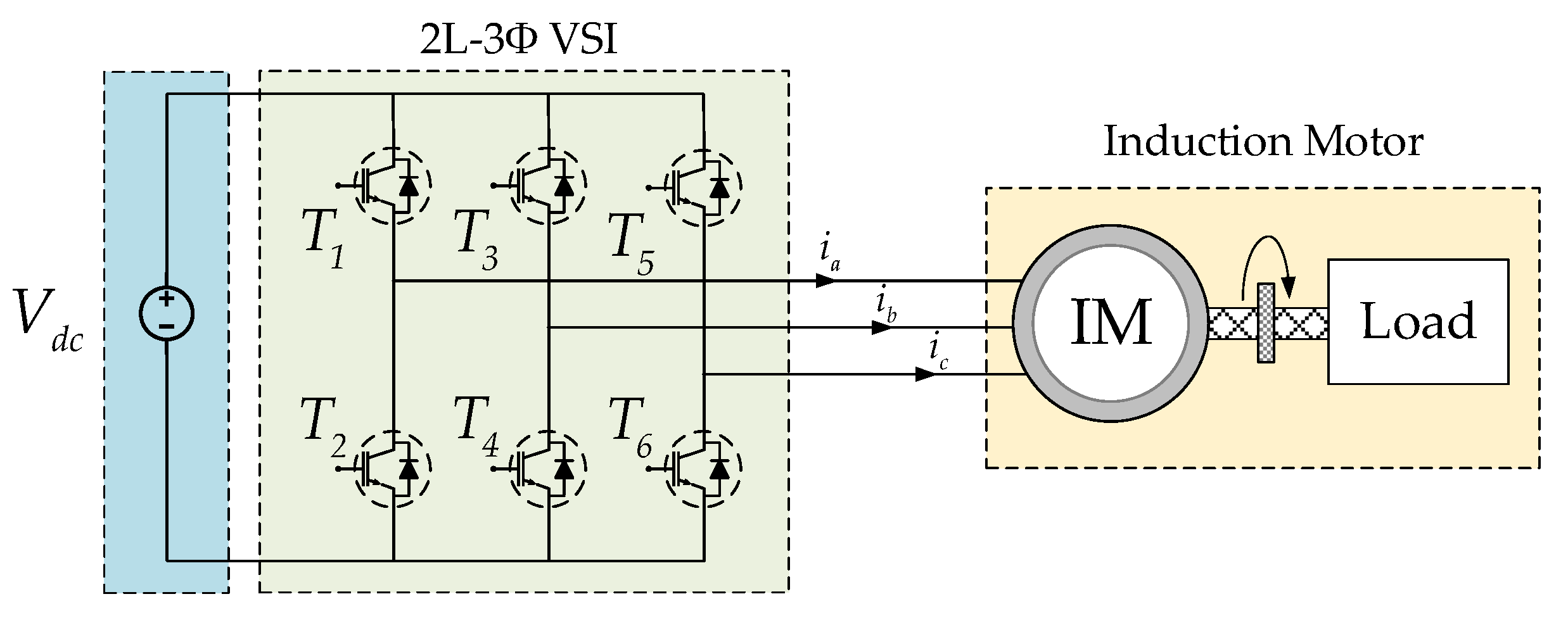
Figure 2.
Sigmoid function for different coefficient values λ.
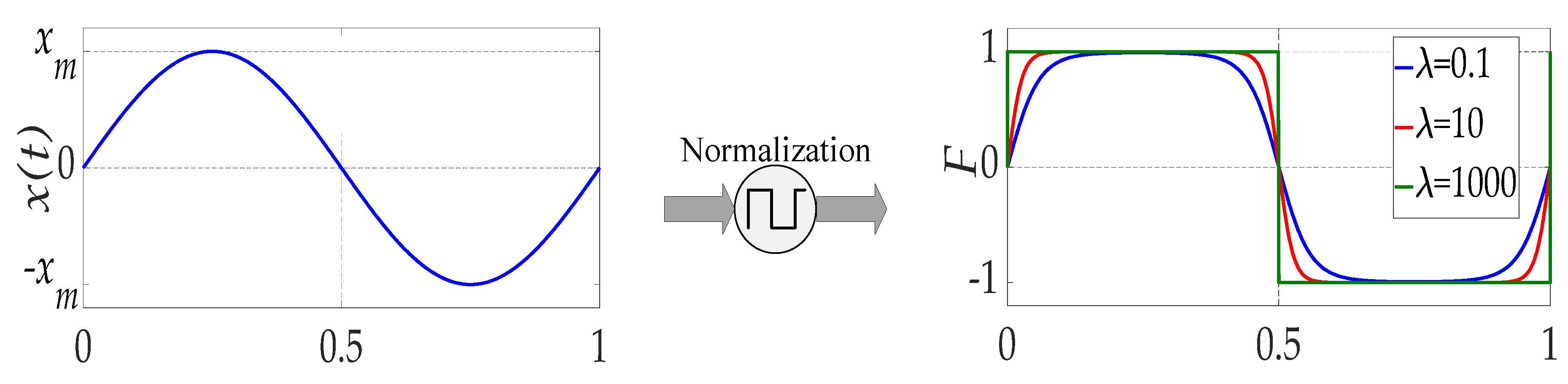
Figure 3.
Current normalization method: (a) with chattering problem, (b) without chattering problem.
Figure 3.
Current normalization method: (a) with chattering problem, (b) without chattering problem.
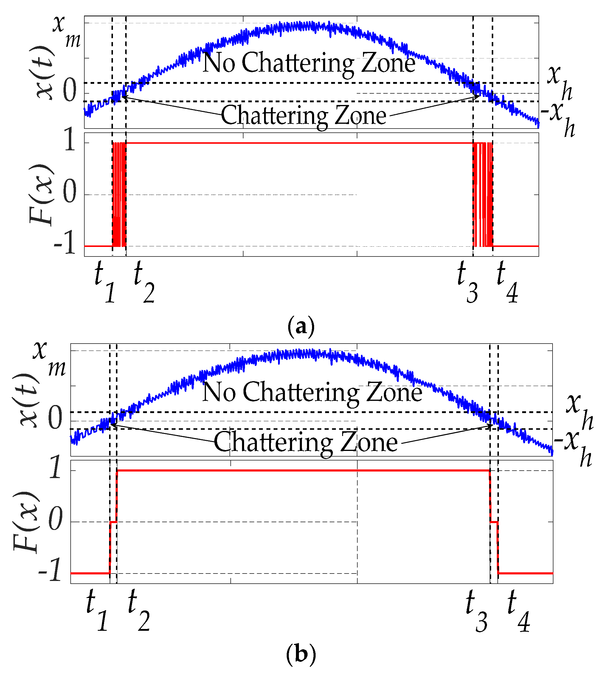
Figure 4.
Time domain waveforms of three phase currents, sigmoid functions and detection fault variables in healthy mode.
Figure 4.
Time domain waveforms of three phase currents, sigmoid functions and detection fault variables in healthy mode.
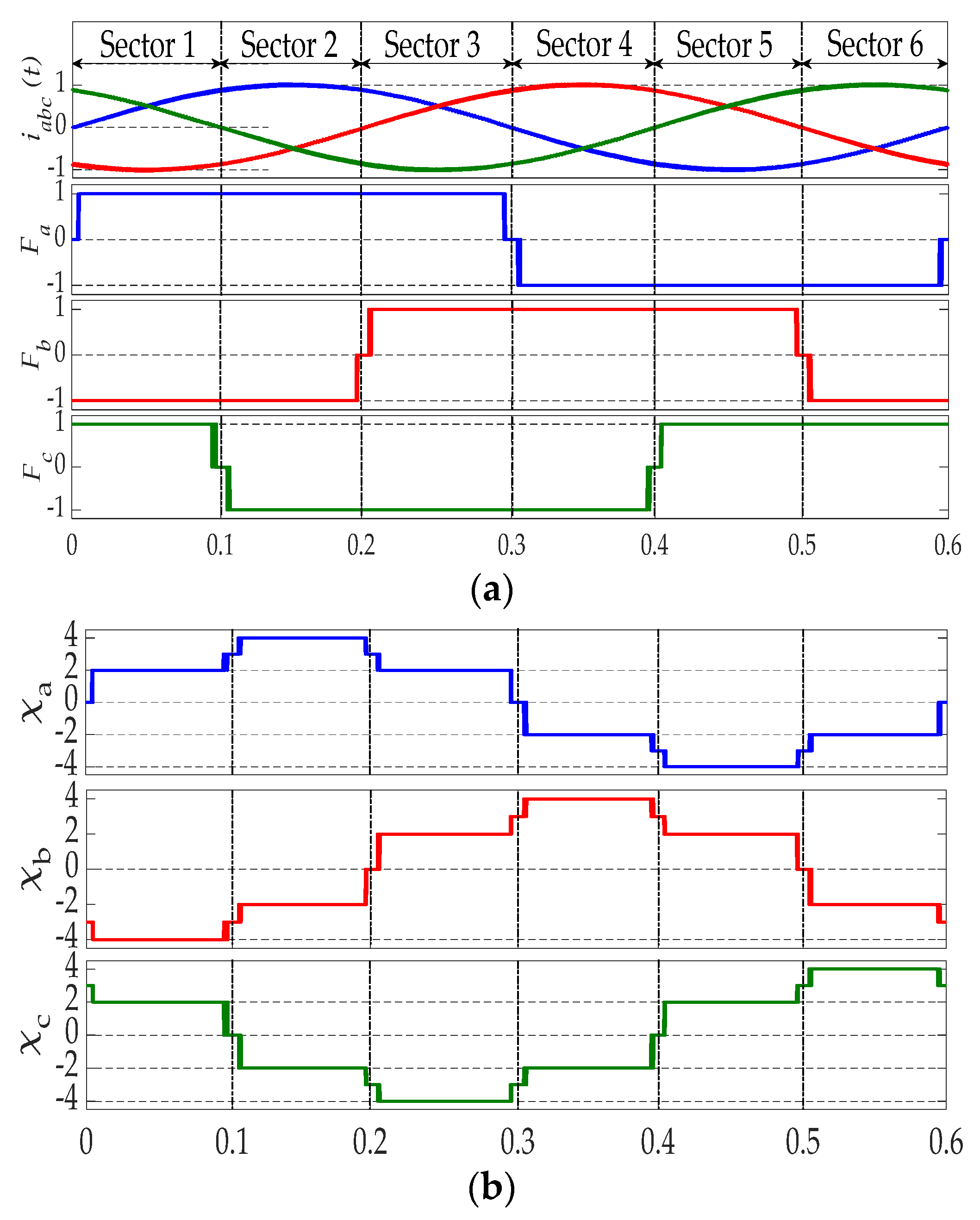
Figure 5.
Time domain waveforms of three phase currents, sigmoïd functions and detection fault variables for: (a) Fault in T1, (b) Fault in T1&T2, (c) Fault in T1&T4.
Figure 5.
Time domain waveforms of three phase currents, sigmoïd functions and detection fault variables for: (a) Fault in T1, (b) Fault in T1&T2, (c) Fault in T1&T4.
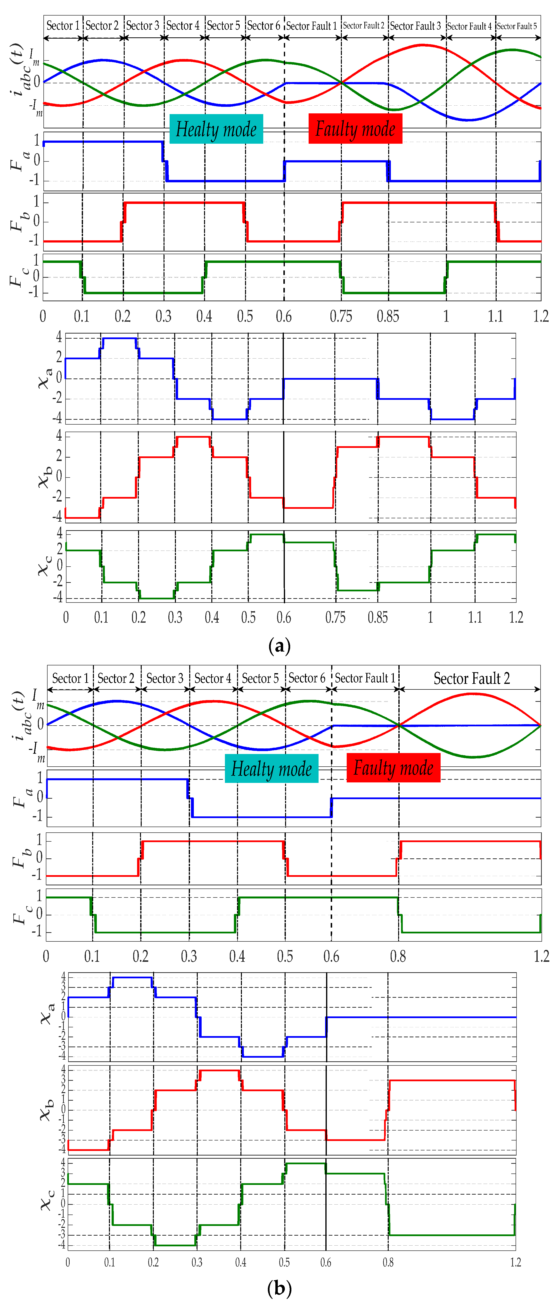
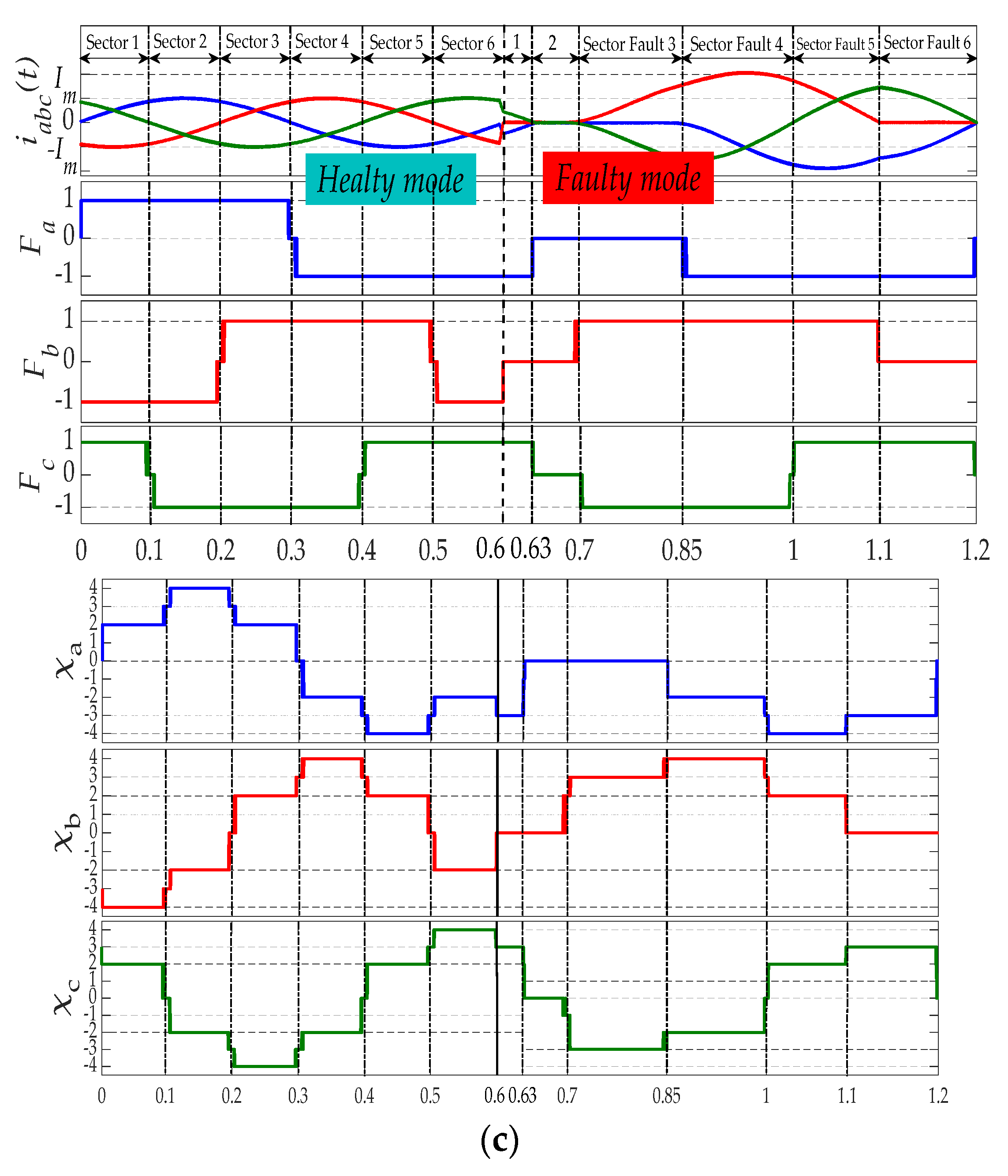
Figure 6.
LSTM Network structure.
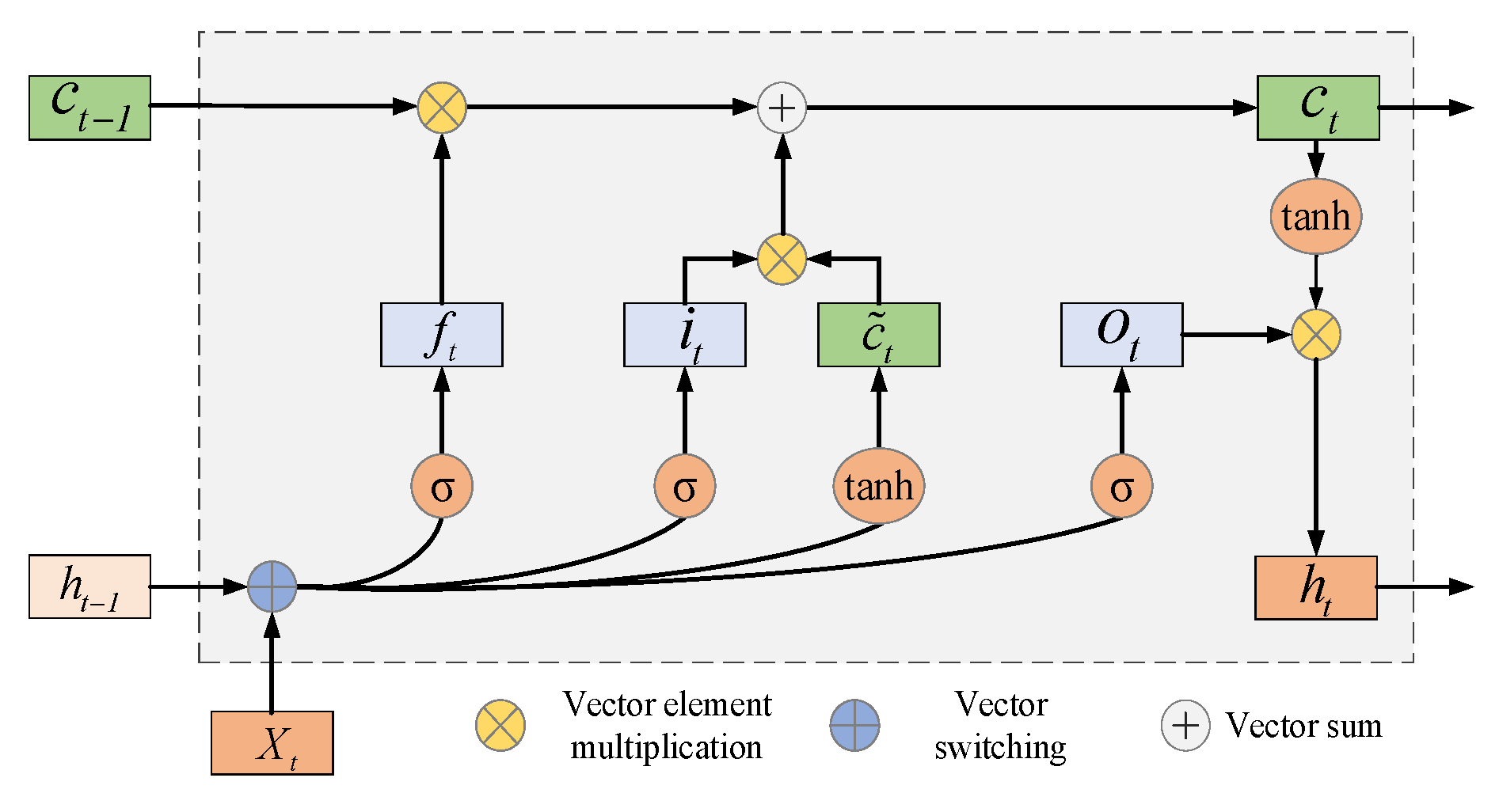
Figure 7.
Stacked LSTM structure.
Figure 8.
BiLSTM structure.
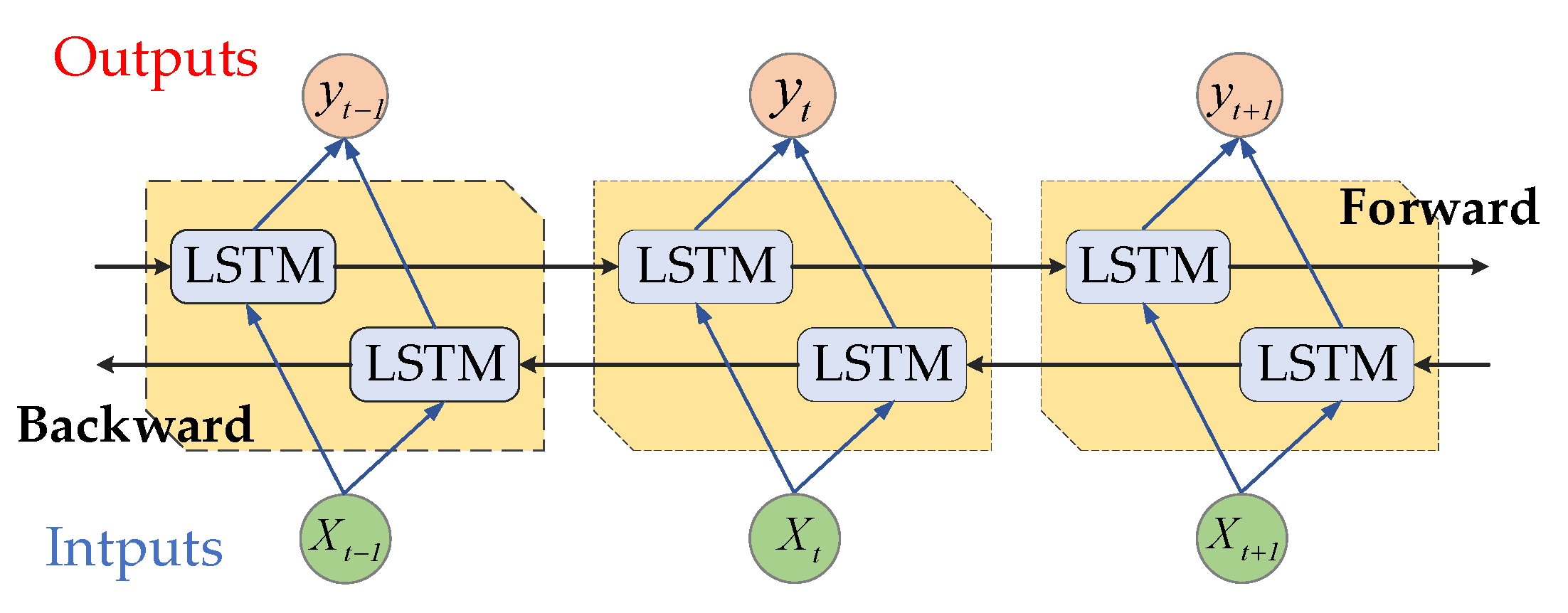
Figure 9.
Structure of the fault diagnosis module based on BiLSTM network.
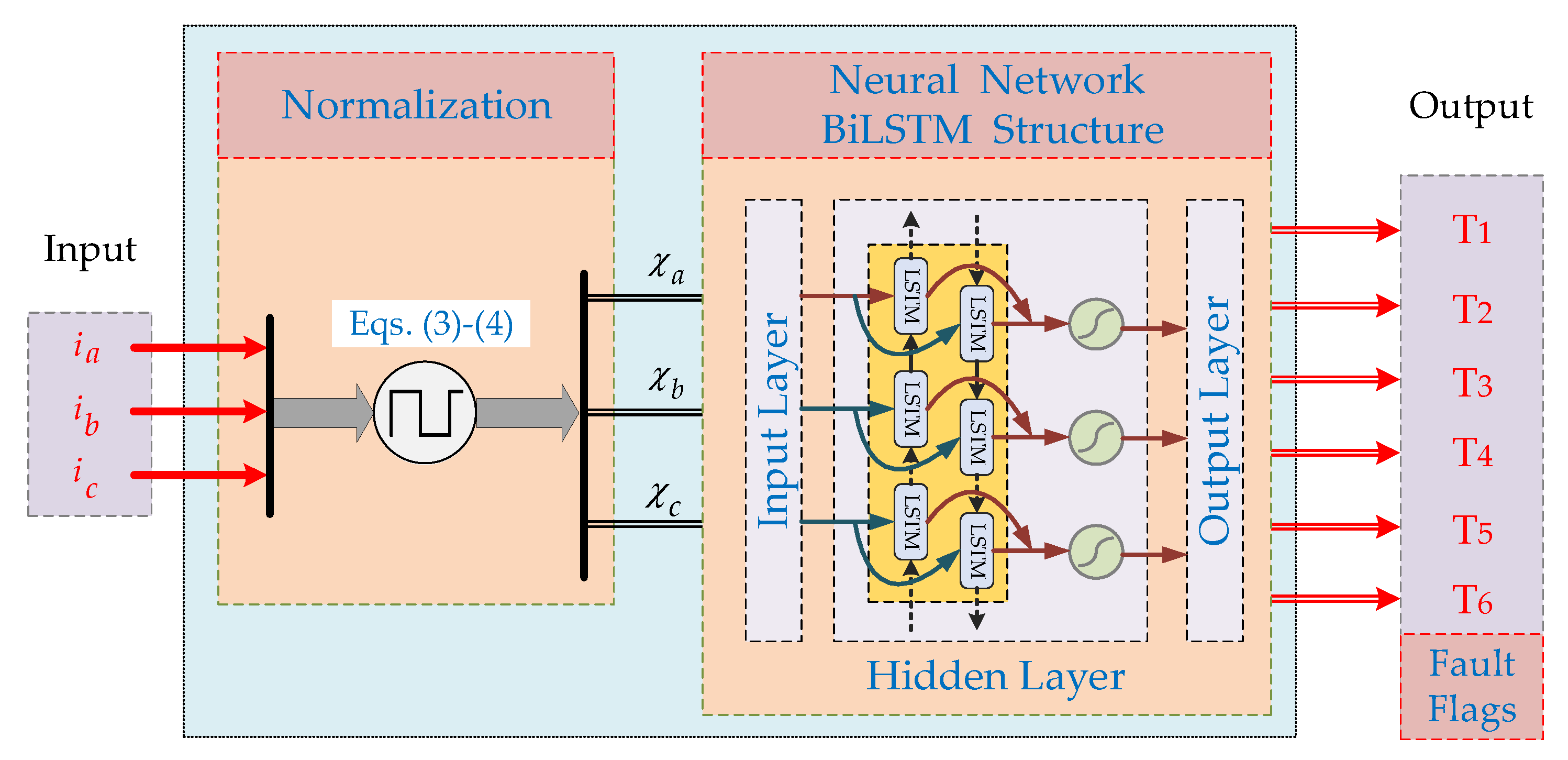
Figure 10.
(a) Evolution of the RMSE as a function of hidden layer size in training progress of BiLSTM Network, (b) Evolution of the Loss as a function of hidden layer size.
Figure 10.
(a) Evolution of the RMSE as a function of hidden layer size in training progress of BiLSTM Network, (b) Evolution of the Loss as a function of hidden layer size.
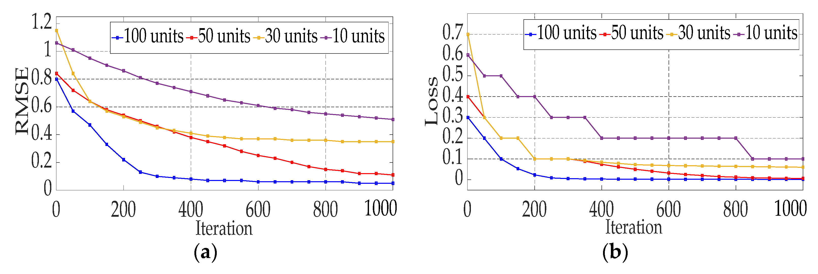
Figure 11.
Simulation results (a) Test of BiLSTM Network in the presence of T5&T6 fault, (b) Validation error of BiLSTM model.
Figure 11.
Simulation results (a) Test of BiLSTM Network in the presence of T5&T6 fault, (b) Validation error of BiLSTM model.
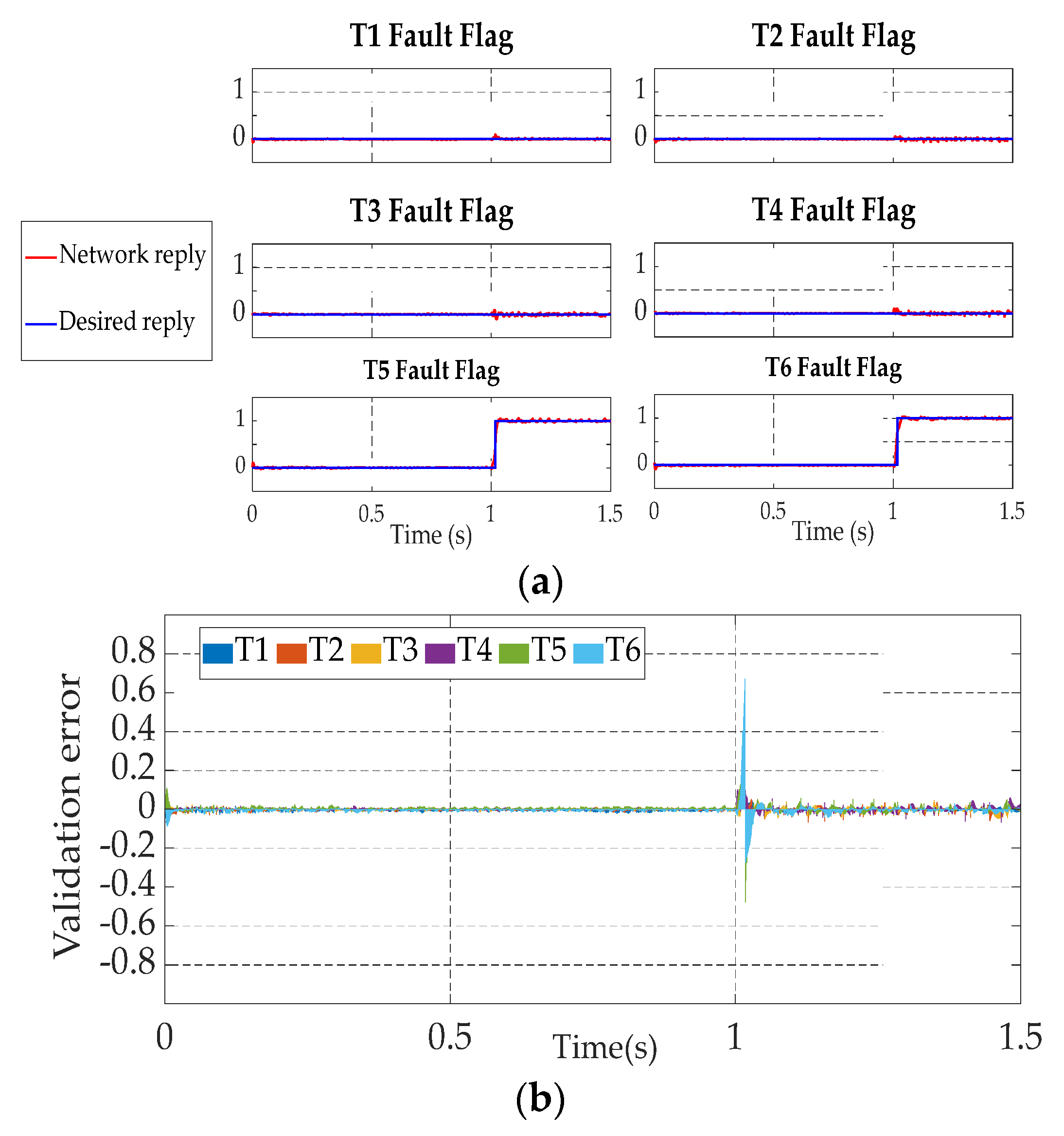
Figure 12.
Simulation results for speed variation from 1200 to 1500rpm without load.
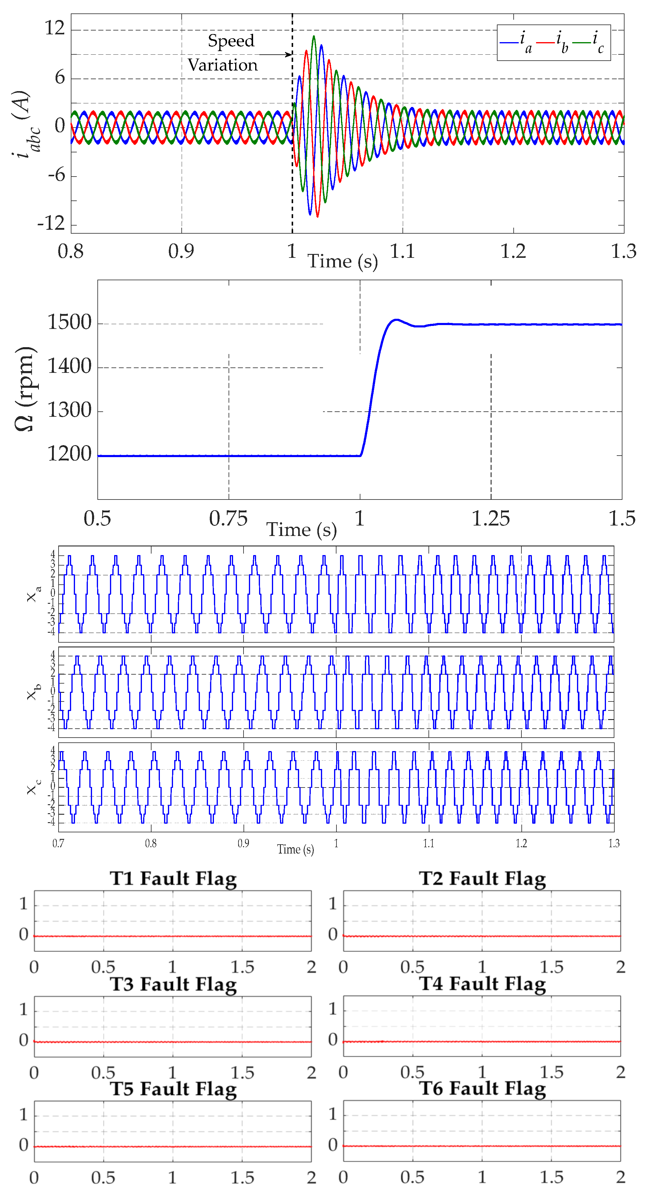
Figure 13.
Simulation results for load variation from 0 to 3N.m under a speed of 1000rpm.
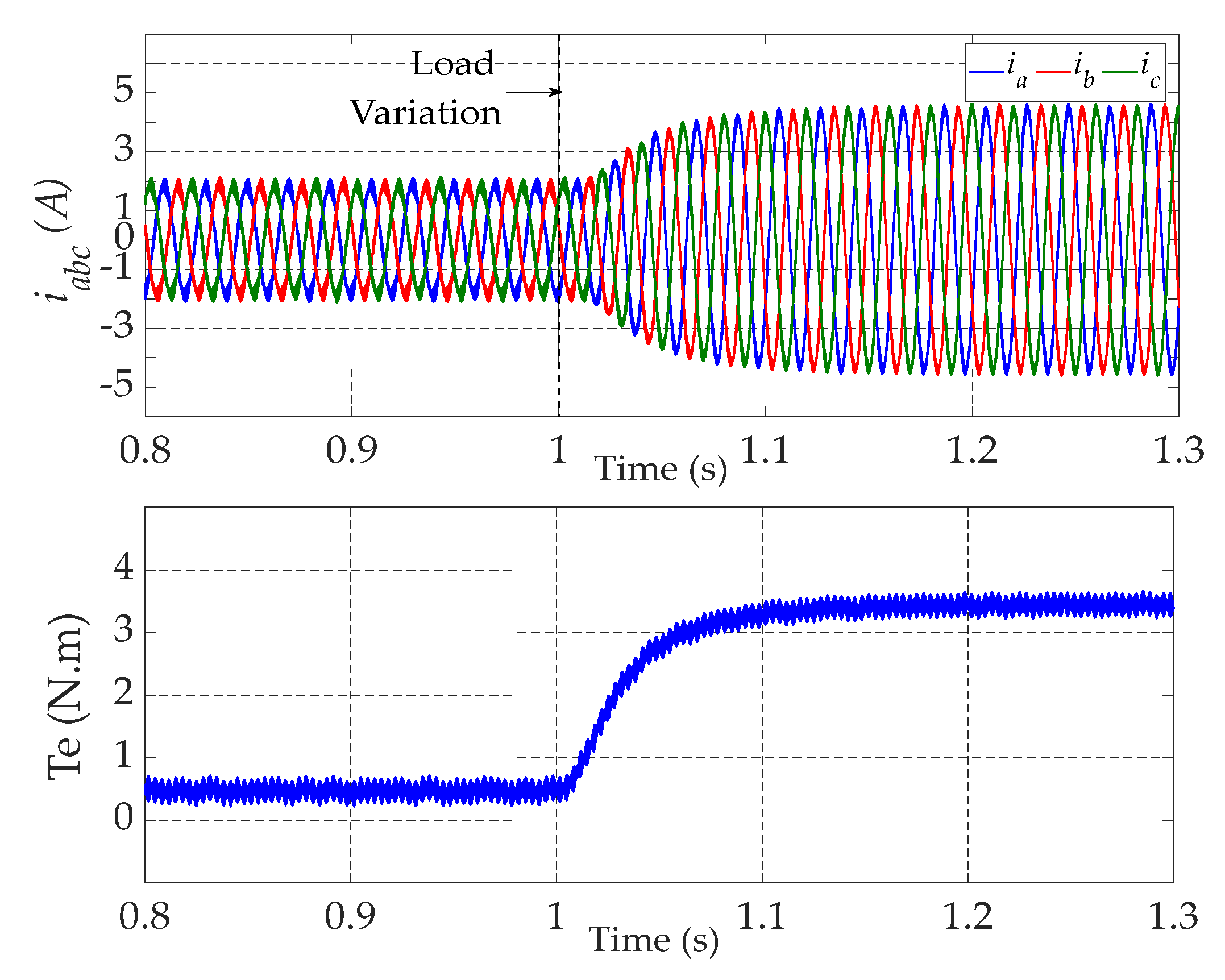
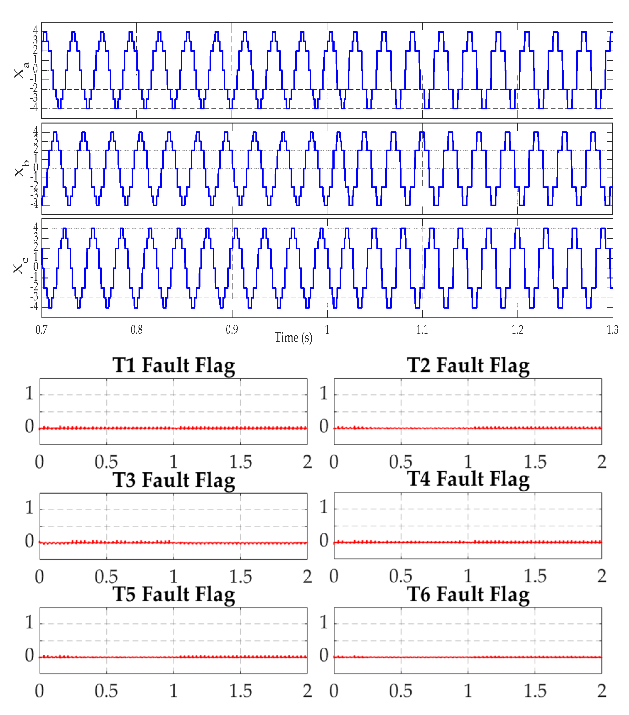
Figure 14.
Simulation results for a fault in T1 under a speed of 800 rpm and a load torque of 4 N.m.
Figure 14.
Simulation results for a fault in T1 under a speed of 800 rpm and a load torque of 4 N.m.
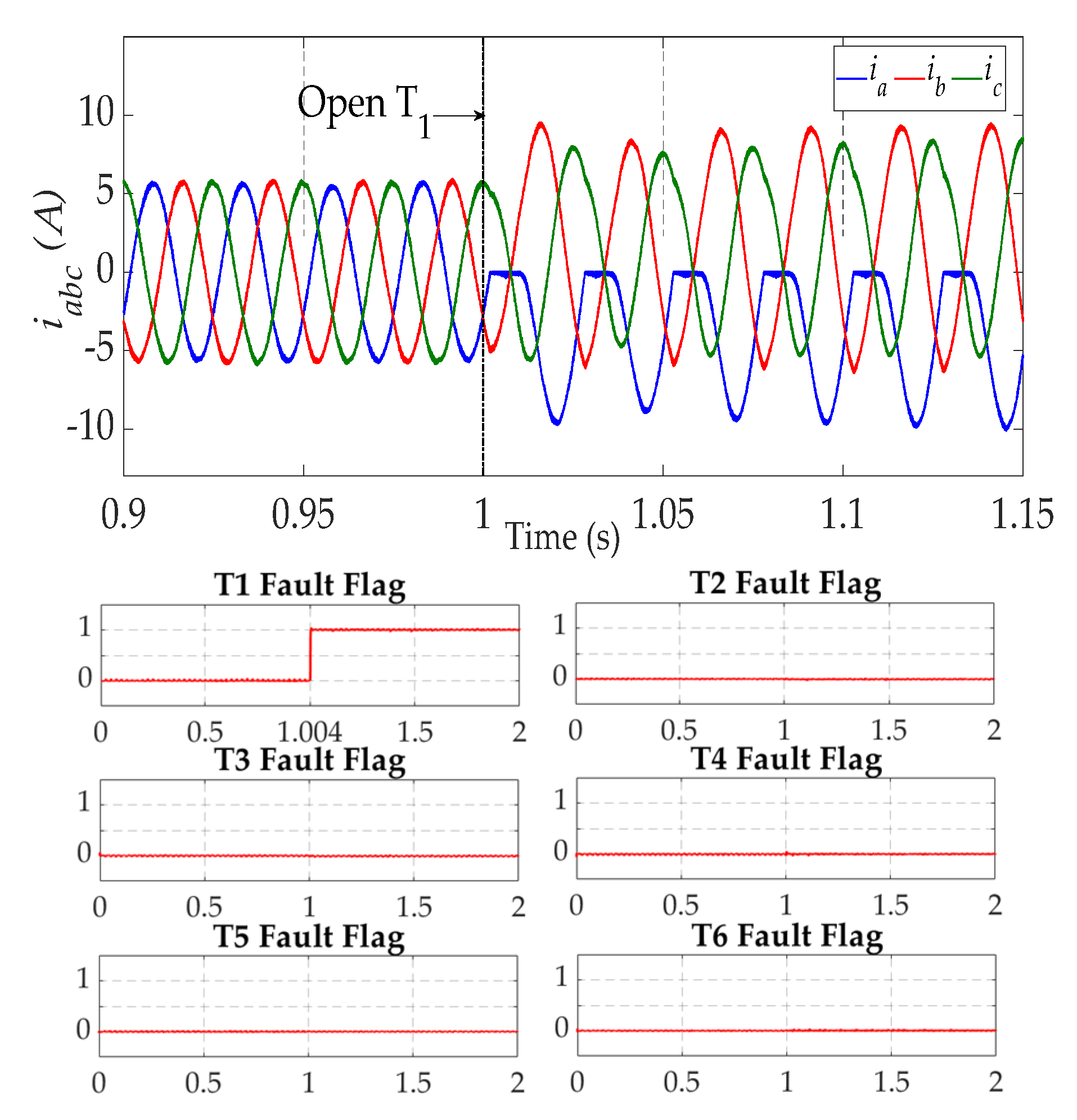
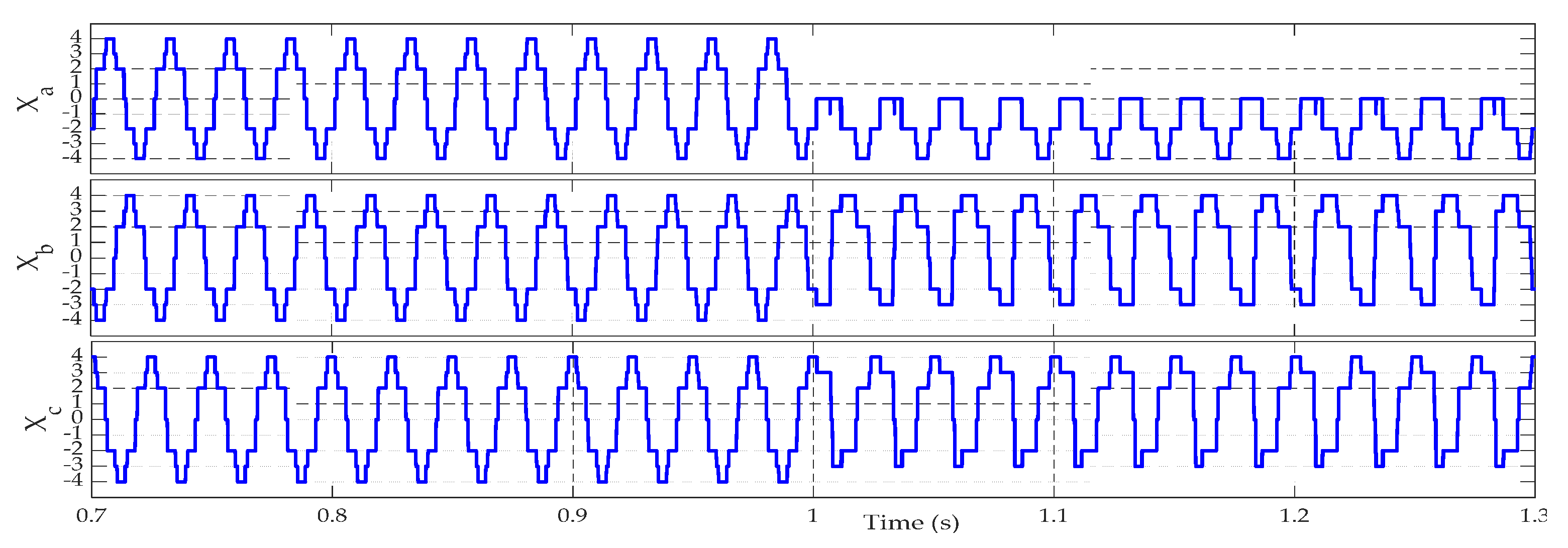
Figure 15.
Simulation results for a fault in T1 and T2 under a speed of 1400 rpm and a load torque of 3 N.m.
Figure 15.
Simulation results for a fault in T1 and T2 under a speed of 1400 rpm and a load torque of 3 N.m.
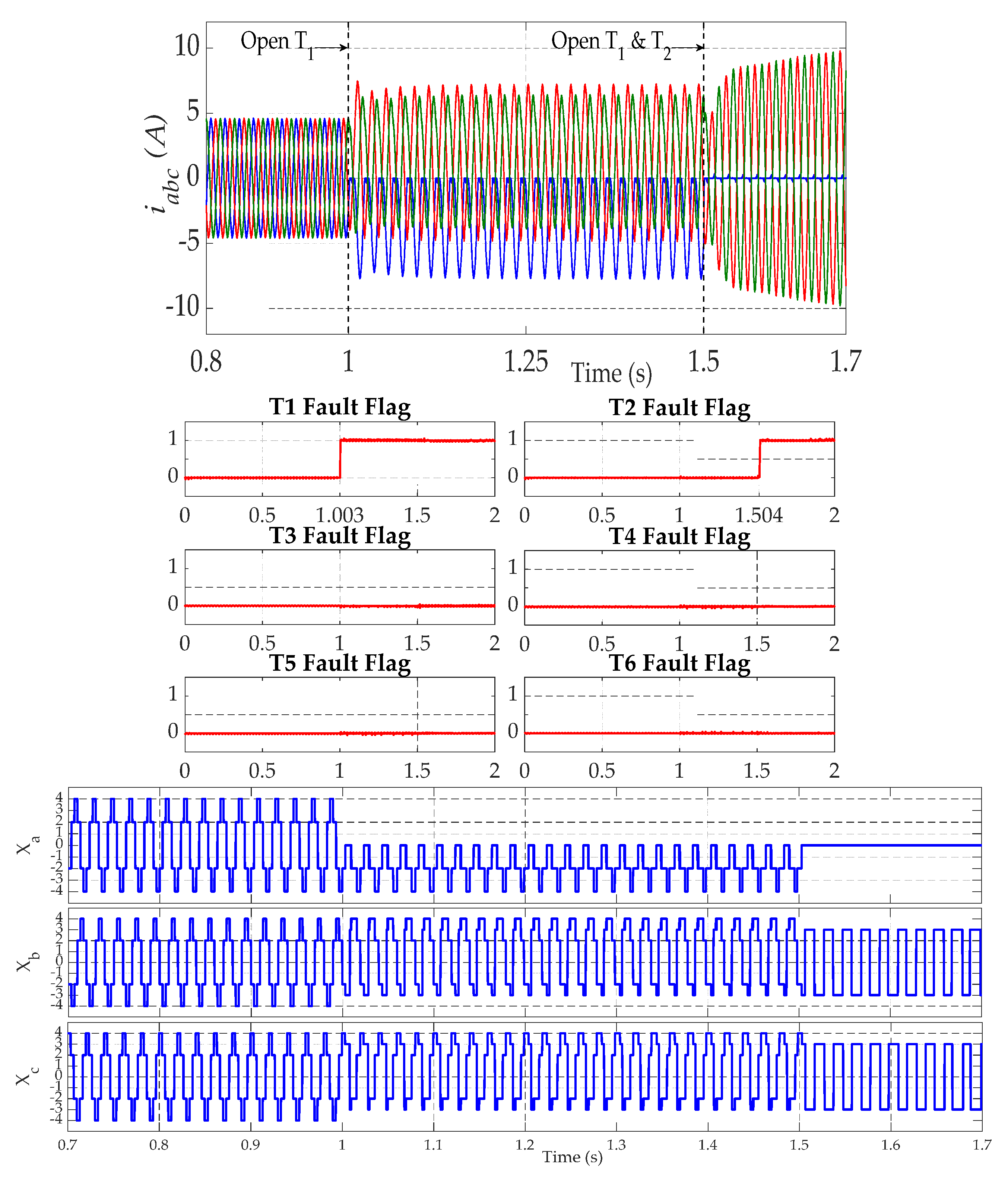
Figure 16.
Simulation results for a fault in T1 and T4 under a speed of 1200 rpm and a load torque of 3 N.m.
Figure 16.
Simulation results for a fault in T1 and T4 under a speed of 1200 rpm and a load torque of 3 N.m.
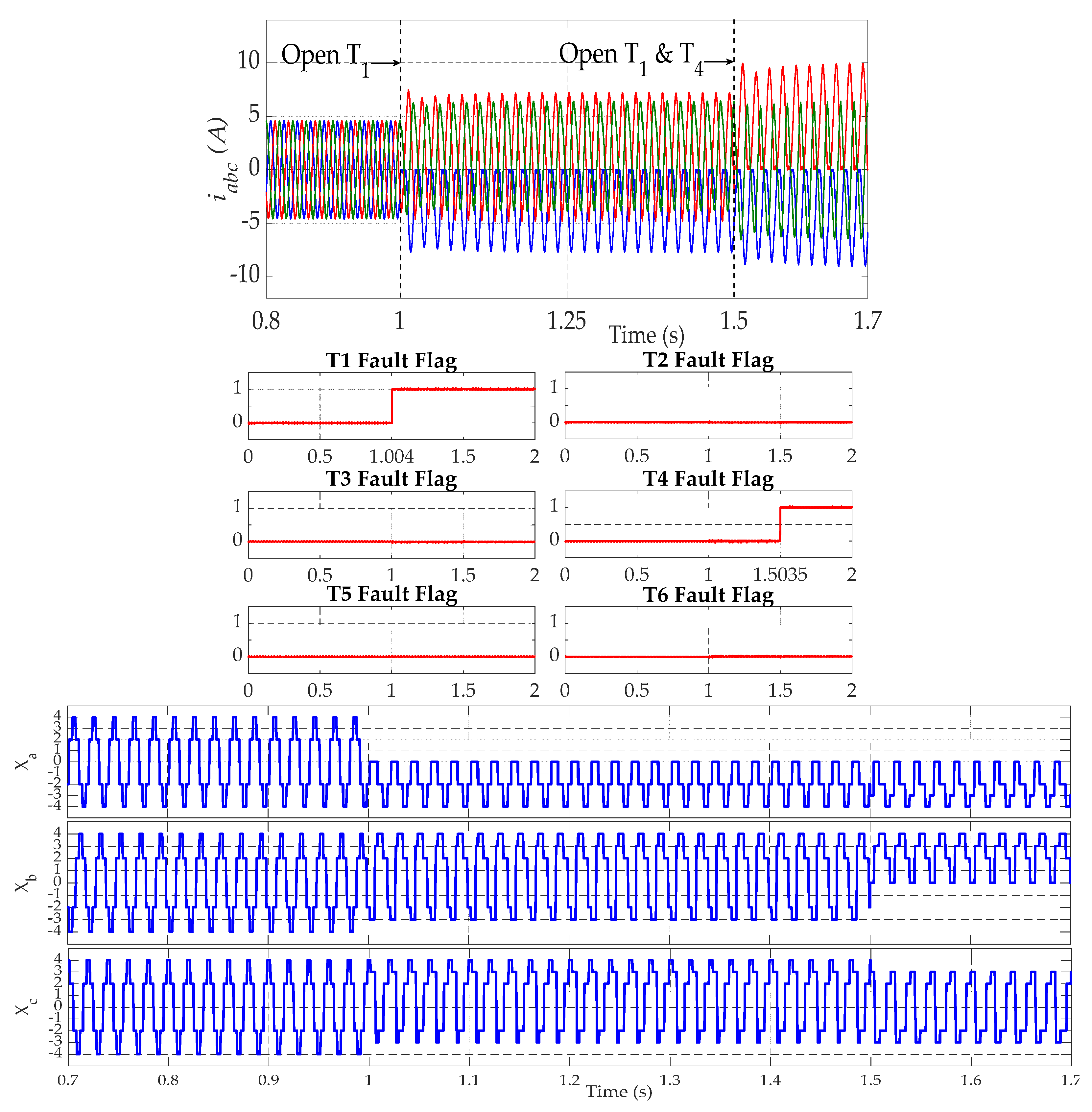
Figure 17.
Experimental test bench.
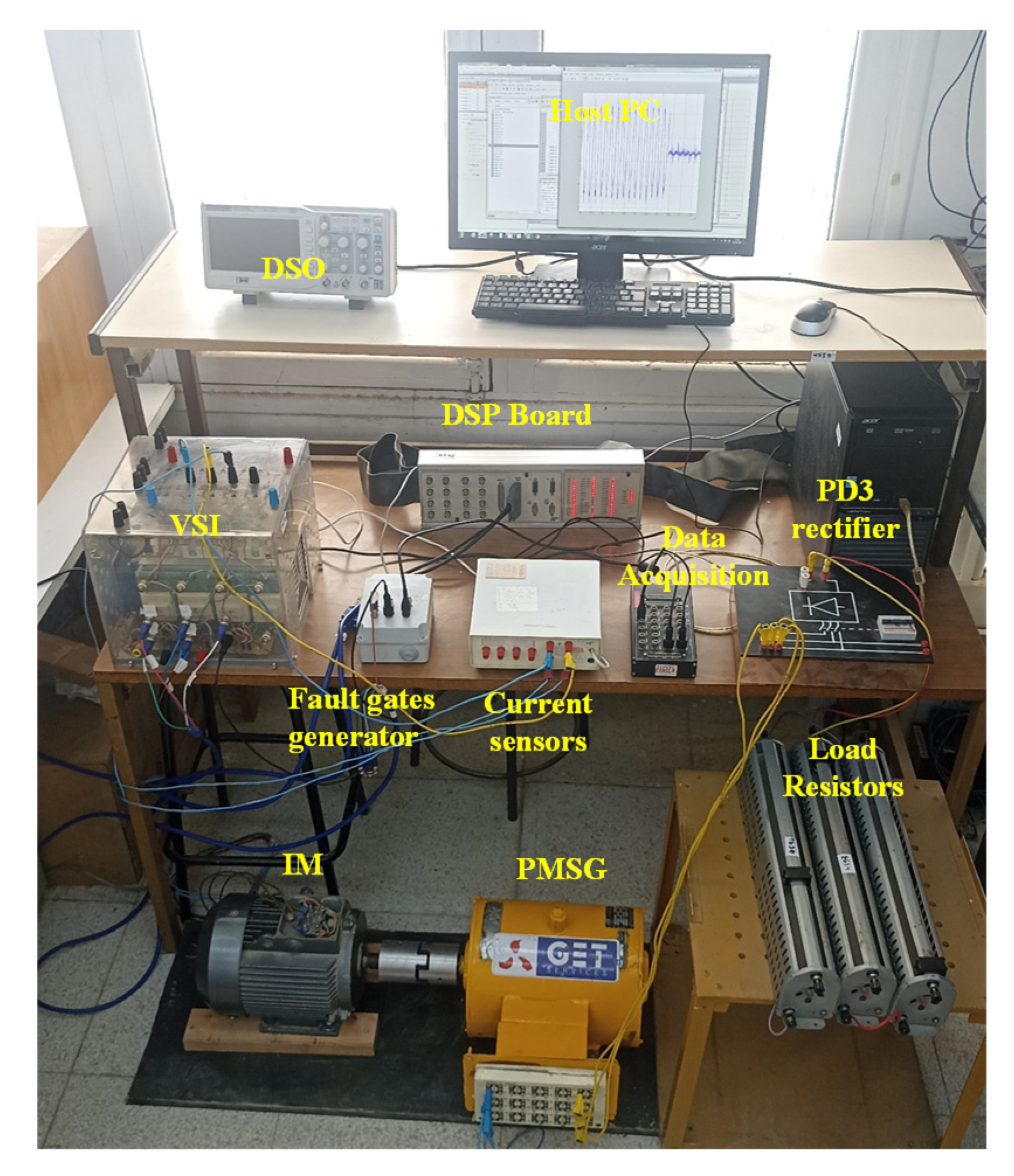
Figure 18.
Experimental results for speed variation from 700 to 1000 rpm with: (a) no load, (b) 60% of rated torque.
Figure 18.
Experimental results for speed variation from 700 to 1000 rpm with: (a) no load, (b) 60% of rated torque.
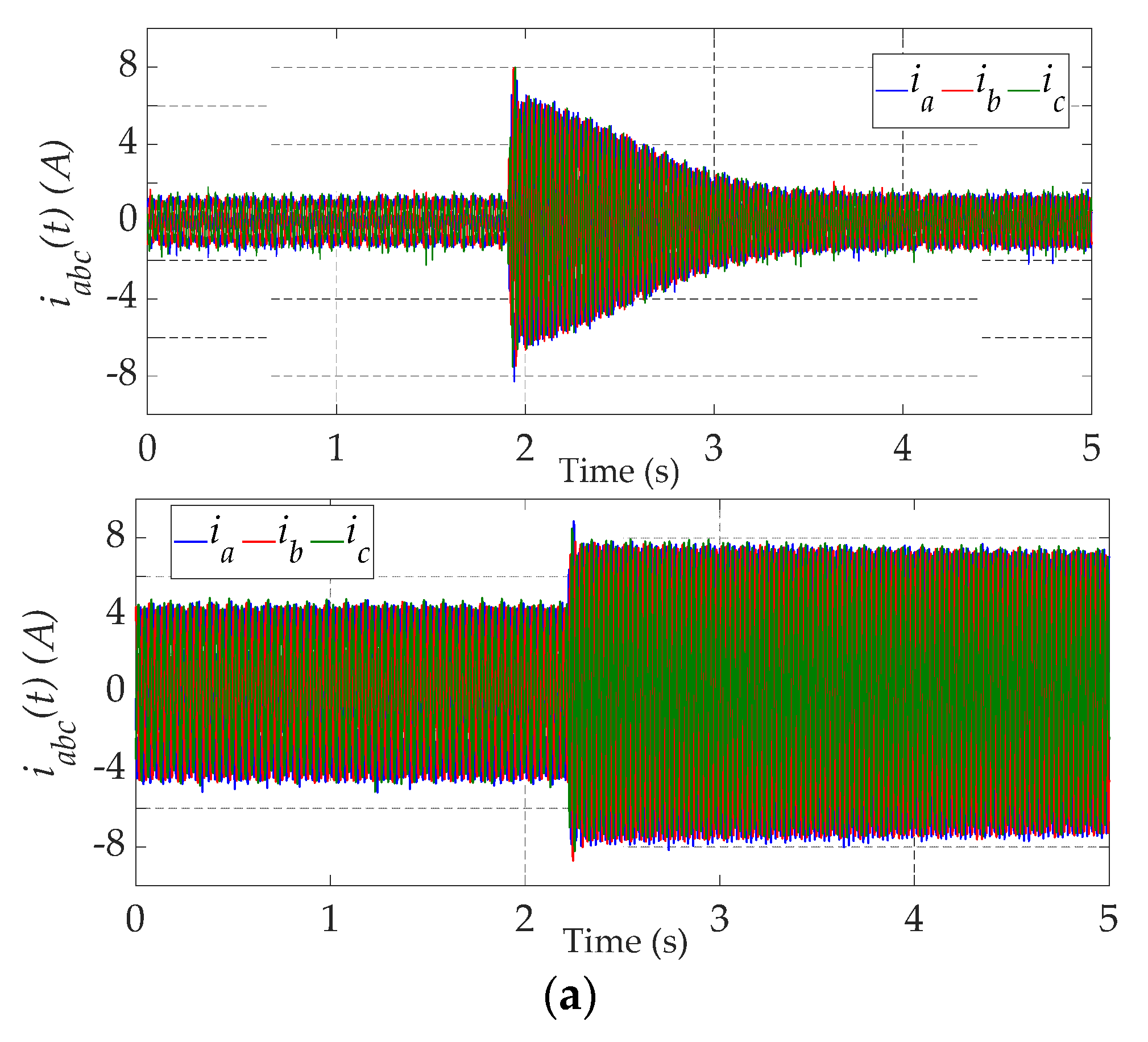
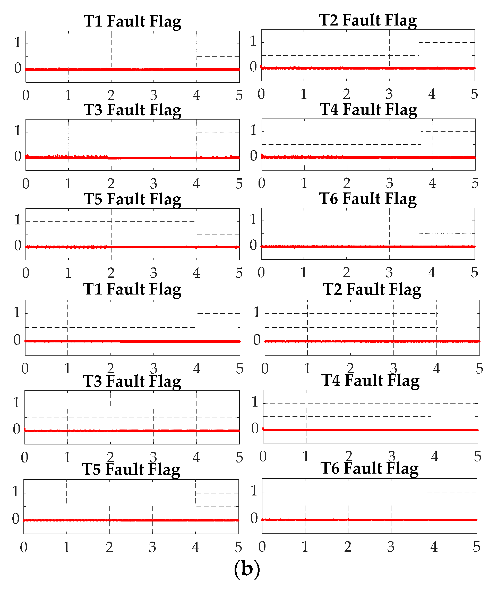
Figure 19.
Experimental results for load variation under a speed of 1000rpm: (a) from 0 to 60% of rated torque, (b) from 60% to 0% of rated torque.
Figure 19.
Experimental results for load variation under a speed of 1000rpm: (a) from 0 to 60% of rated torque, (b) from 60% to 0% of rated torque.
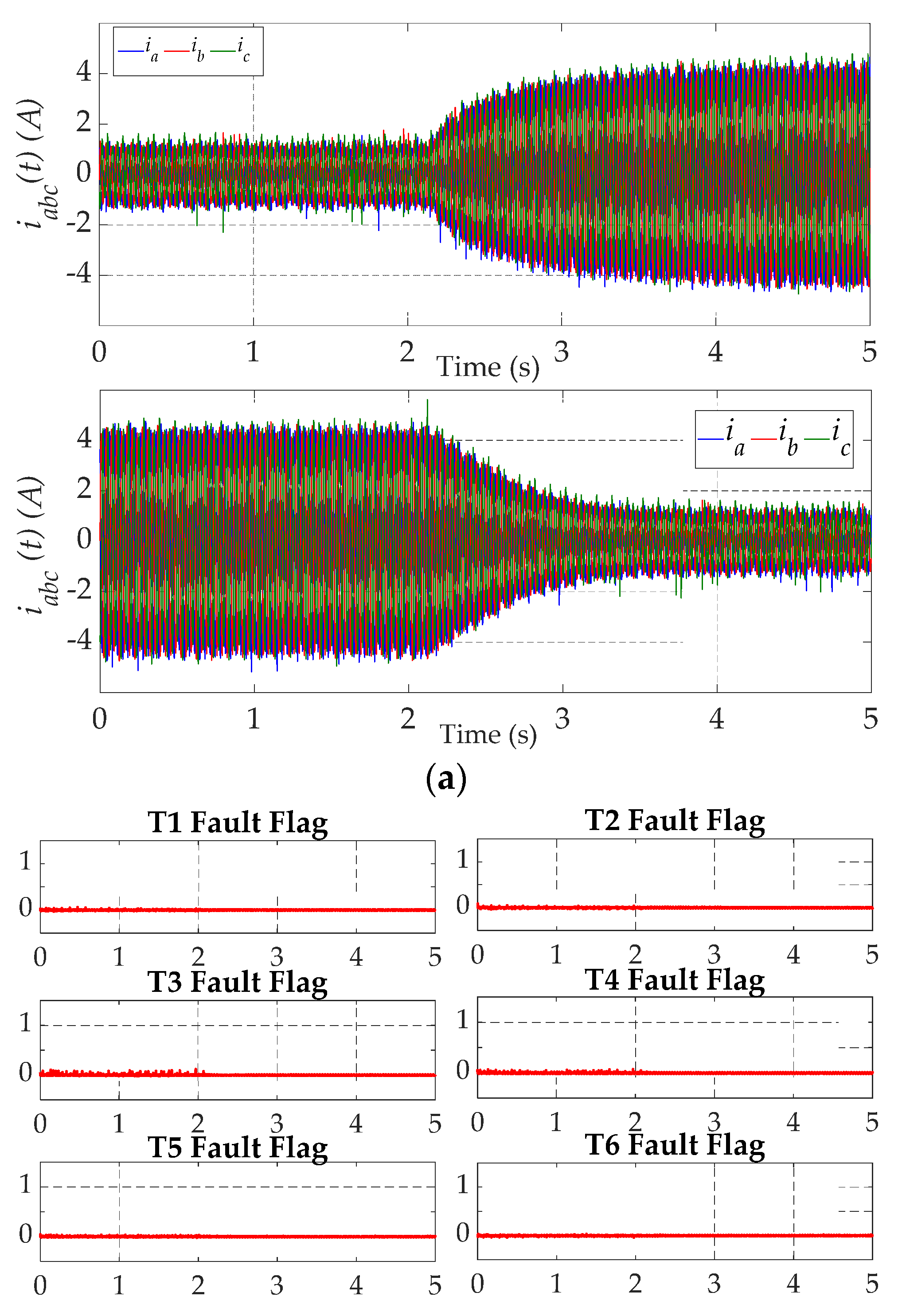
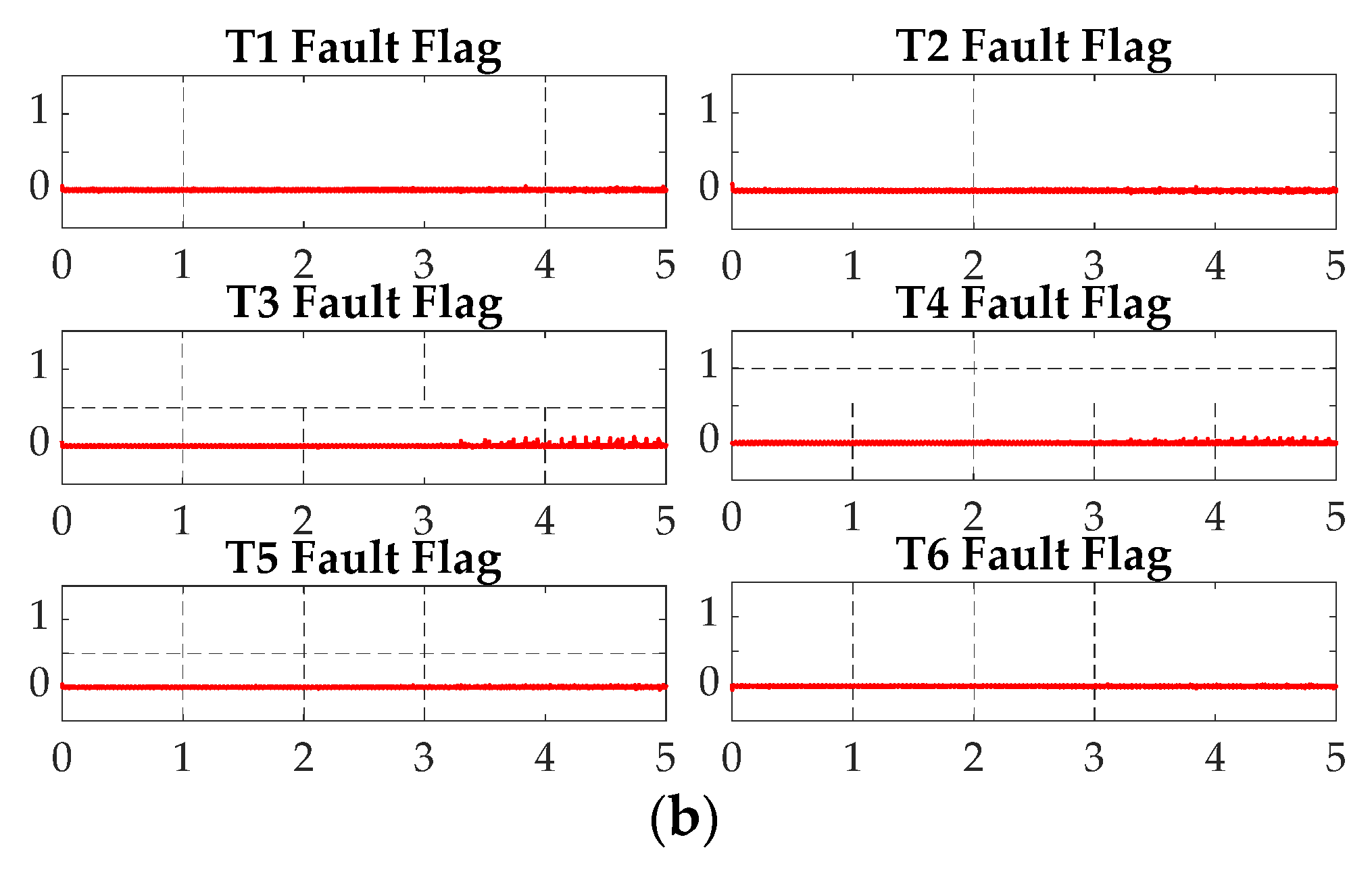
Figure 20.
Experimental results for a fault in T3 under a speed of 780 rpm and 50% of rated torque.
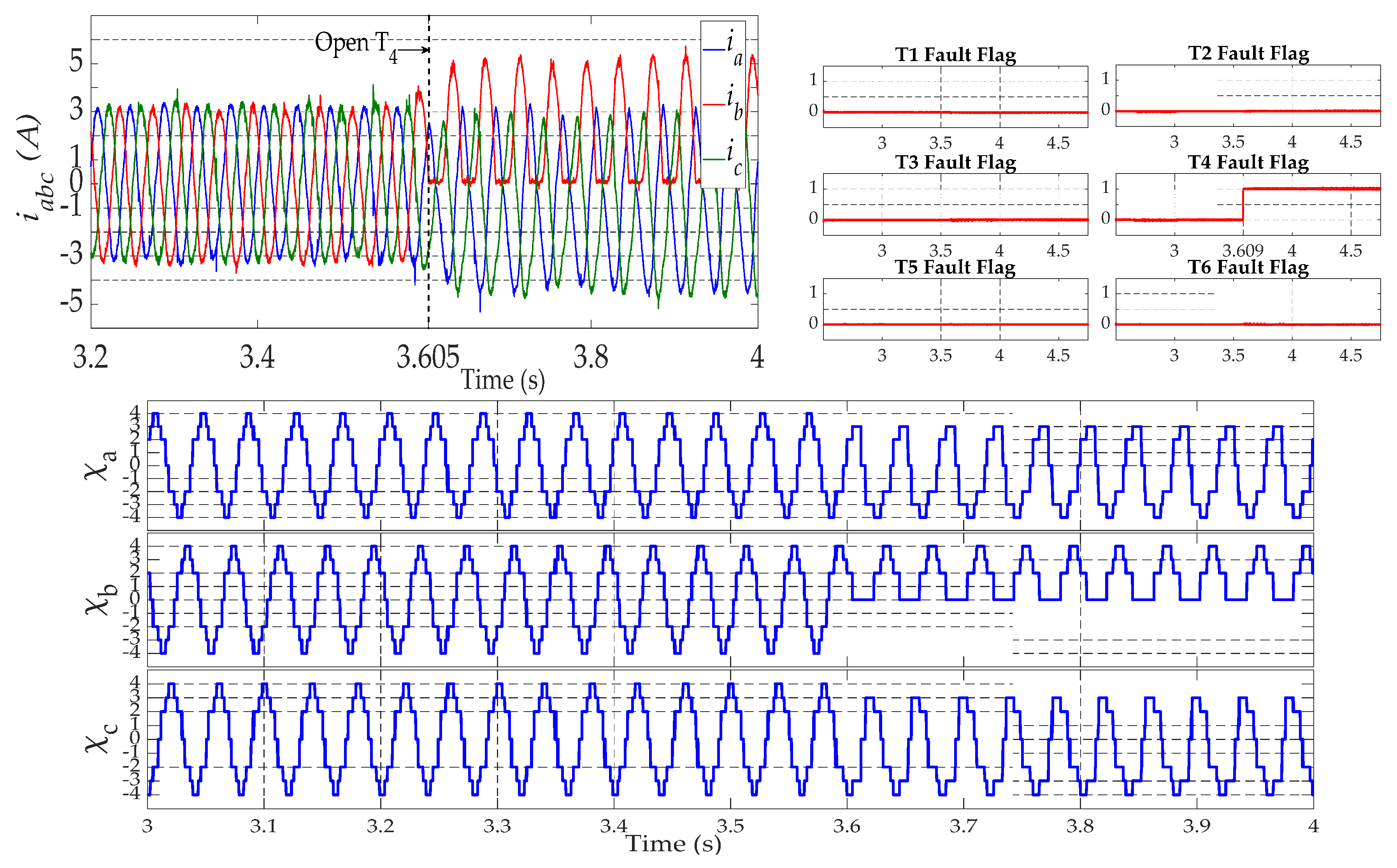
Figure 21.
Experimental results for a double fault in T1 and T2 under a speed of 990 rpm and 50% of load.
Figure 21.
Experimental results for a double fault in T1 and T2 under a speed of 990 rpm and 50% of load.
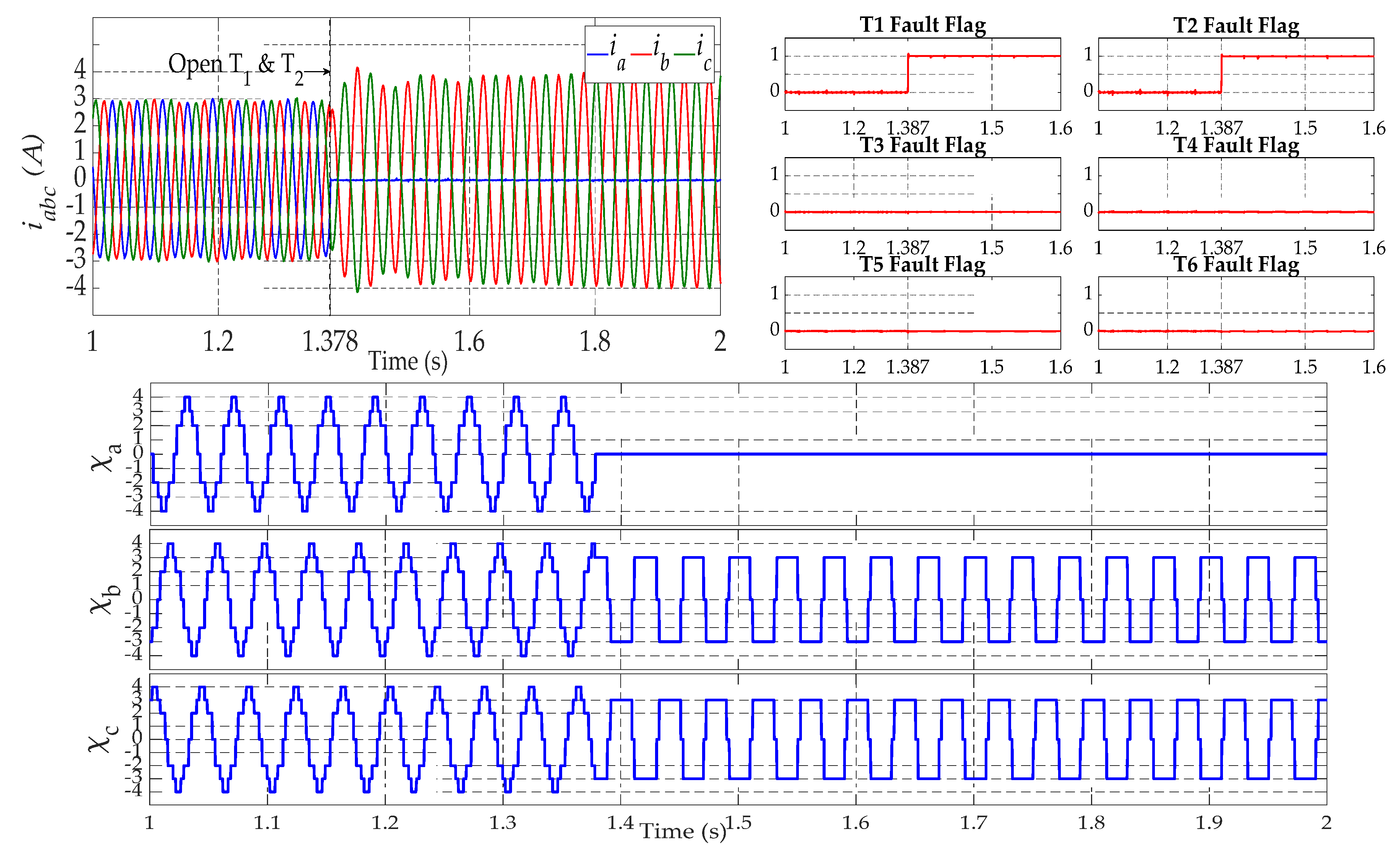
Figure 22.
Experimental results for a double fault in T2 and T3 under a speed of 1000 rpm and no load.
Figure 22.
Experimental results for a double fault in T2 and T3 under a speed of 1000 rpm and no load.
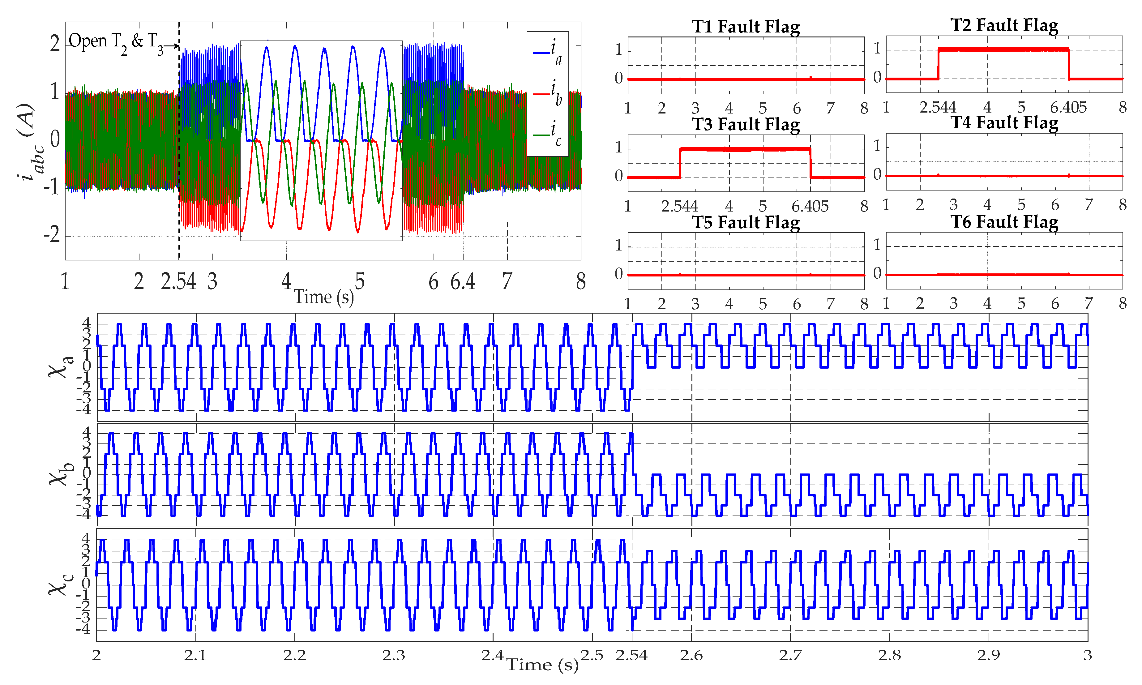
Figure 23.
MAE evolution when open-circuit switch fault happens on T1&T2 for the BiLSTM and the other comparison methods.
Figure 23.
MAE evolution when open-circuit switch fault happens on T1&T2 for the BiLSTM and the other comparison methods.
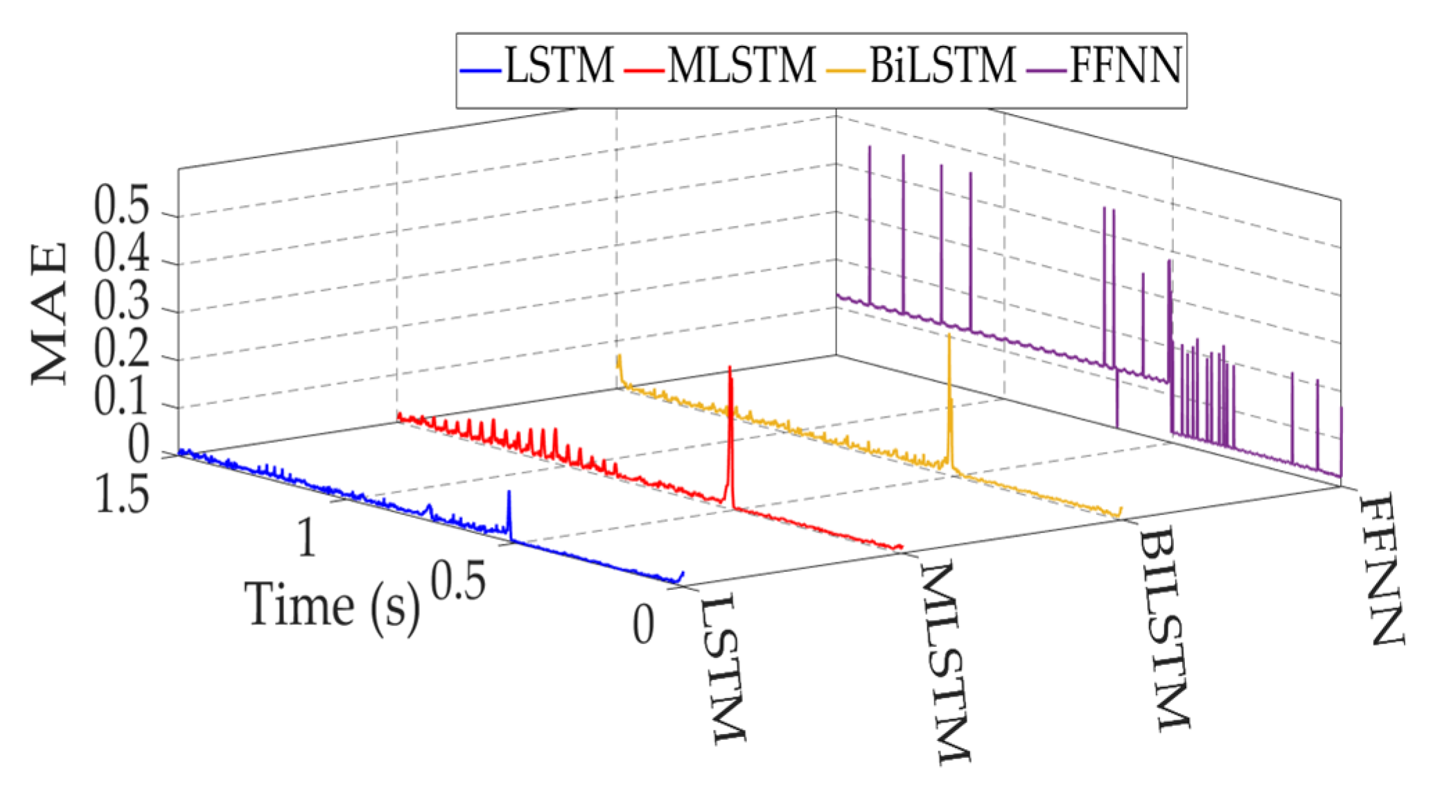
Figure 24.
Performance evolution: RMSE evolution for each faults (T1,T2,T3,T4,T5,T6) when open-circuit switch fault happens on T1&T2 for the BiLSTM and the other comparison methods.
Figure 24.
Performance evolution: RMSE evolution for each faults (T1,T2,T3,T4,T5,T6) when open-circuit switch fault happens on T1&T2 for the BiLSTM and the other comparison methods.
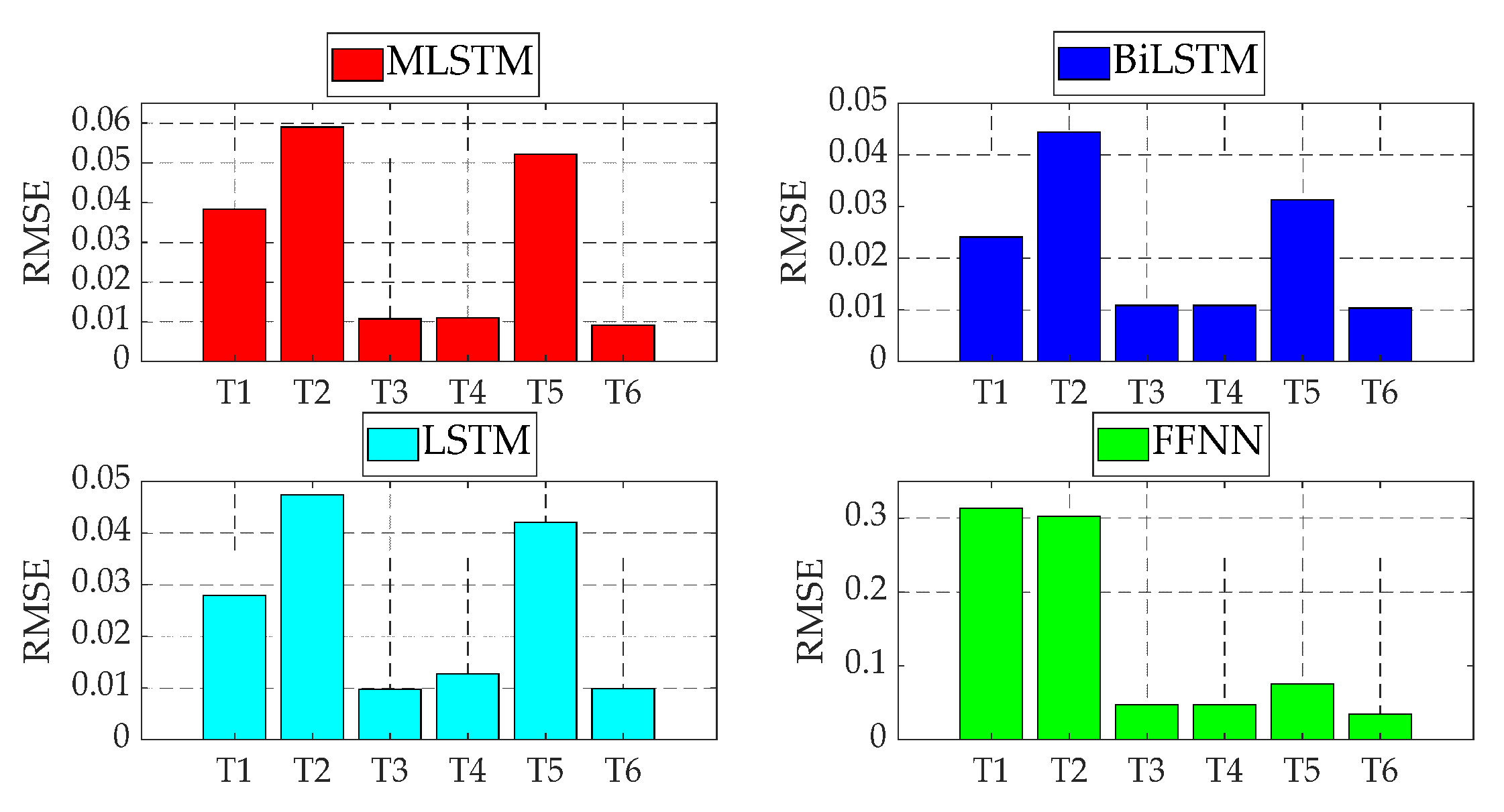

Table 1.
LSTM parameter.
| Parameter | Value |
|---|---|
| Max training epochs | 1000 |
| Loss function optimizer (solver) | Adam |
| Initial learning rate | 0.001 |
| Loss function | RMSE |
| Gradient Threshold | 0.001 |
| Hidden units | 100 |
Table 2.
Performance evaluation for each method.
| Faulty Switch | FFNN | LSTM | MLSTM (3 layers) | BiLSTM | ||||||||||||
|---|---|---|---|---|---|---|---|---|---|---|---|---|---|---|---|---|
| RMSE | MAE | Td (ms) | Accuracy(%) | RMSE | MAE | Td (ms) | Accuracy(%) | RMSE | MAE | Td (ms) | Accuracy(%) | RMSE | MAE | Td (ms) | Accuracy(%) | |
| T1 | 0.2073 | 0.1268 | 1 | 32.9996 | 0.0142 | 0.0093 | 11.5 | 97.8281 | 0.0150 | 0.0101 | 11 | 97.5032 | 0.0135 | 0.0095 | 3.45 | 98.2613 |
| T2 | 0.2002 | 0.1241 | 1.1 | 34.4586 | 0.0209 | 0.0128 | 21 | 96.5231 | 0.0207 | 0.0137 | 23 | 95.7970 | 0.0192 | 0.0128 | 5.2 | 96.5596 |
| T3 | 0.1915 | 0.1222 | 1 | 34.8000 | 0.0186 | 0.0116 | 23 | 96.5823 | 0.0174 | 0.0094 | 24 | 96.8548 | 0.0178 | 0.0116 | 6 | 97.3394 |
| T4 | 0.1977 | 0.1241 | 1 | 33.5121 | 0.0160 | 0.0105 | 16 | 97.3179 | 0.0157 | 0.0102 | 13.5 | 97.5014 | 0.0146 | 0.0099 | 4.88 | 97.9273 |
| T5 | 0.1983 | 0.1235 | 1 | 33.8192 | 0.0167 | 0.0107 | 21 | 97.3560 | 0.0192 | 0.0121 | 24 | 95.1774 | 0.0158 | 0.0098 | 2.5 | 98.1525 |
| T6 | 0.2061 | 0.1242 | 1 | 33.6194 | 0.0162 | 0.0102 | 12 | 97.4939 | 0.0149 | 0.0092 | 13 | 97.0993 | 0.0132 | 0.0089 | 4.02 | 97.8641 |
| T1&T2 | 0.1369 | 0.0935 | 1 | 74.1148 | 0.0250 | 0.0109 | 14 | 98.5637 | 0.0300 | 0.0132 | 17 | 98.1124 | 0.0220 | 0.0105 | 2.57 | 98.8193 |
| T3&T4 | 0.1242 | 0.0775 | 1 | 75.8453 | 0.0244 | 0.0112 | 24 | 98.2274 | 0.0270 | 0.0126 | 19 | 96.8244 | 0.0253 | 0.0109 | 4.66 | 98.3066 |
| T5&T6 | 0.1304 | 0.0796 | 1 | 76.2560 | 0.0302 | 0.0092 | 10 | 99.3372 | 0.0278 | 0.0101 | 16 | 99.2203 | 0.0302 | 0.0101 | 3.75 | 99.4112 |
| Mean | 0.1769 | 0.1108 | 1.0111 | 47.7139 | 0.0202 | 0.0107 | 16.94 | 97.6922 | 0.0208 | 0.0111 | 17.83 | 97.1211 | 0.019 | 0.0104 | 4.11 | 98.07 |
| The bold values represent optimum evaluation metrics | ||||||||||||||||
Table 3.
Comparative study.
| References | Method | Detection Time * |
Accuracy (%) |
|---|---|---|---|
| Maamouri et al. [13] | System model based Sliding Mode Observer (SMO) | 20% | -- |
| Gmati et al. [23] | Predictive current errors and Fuzzy Logic approach | 12-75% | -- |
| Chen et al. [28] | Output line voltage residuals | 5-83% | -- |
| Gou et al. [31] | Online data-driven based Random vector functional link (RVFL) | 110% | 98.83% |
| Xia et al. [33] | Machine learning based transferrable data-driven method | 100% | 96.76% |
| Xue et al. [36] | Classification open circuit faults based LSTM network | 12% | 94% |
| Proposed approach | Prediction open circuit faults based BiLSTM network | 12-30% | 98.08% |
*: % of the current fundamental period.
Disclaimer/Publisher’s Note: The statements, opinions and data contained in all publications are solely those of the individual author(s) and contributor(s) and not of MDPI and/or the editor(s). MDPI and/or the editor(s) disclaim responsibility for any injury to people or property resulting from any ideas, methods, instructions or products referred to in the content. |
© 2023 by the authors. Licensee MDPI, Basel, Switzerland. This article is an open access article distributed under the terms and conditions of the Creative Commons Attribution (CC BY) license (http://creativecommons.org/licenses/by/4.0/).
Copyright: This open access article is published under a Creative Commons CC BY 4.0 license, which permit the free download, distribution, and reuse, provided that the author and preprint are cited in any reuse.


