
Submitted:
16 November 2023
Posted:
17 November 2023
You are already at the latest version
Abstract
Fabry-Pérto (FP) cavity is the essential component of ultra-stable laser (USL) for gravitational wave detection, which couples multi-physic (Optical/Thermal/Mechanics) fields and requires ultra-high precision. To satisfy the requirements of precise and efficient design, a multi-physic coupling optimization method for fixing cubic FP cavity based on data learning is proposed. A multi-physic model for the cubic FP cavity is established and the performance is obtained by finite element analysis. The key performance indices (V, wF, wF) and key design variables (d, l, F) are determined considering the features of the FP cavity. The 49 sets of data by orthogonal experiment are acquired for the establishment and comparison of different data learning models (NN, RSF, KRG). The result turns out that the neural network has the best performance. Based on NSGA-II, the Pareto optimal front is obtained and the optimal combination of design variables is finally determined as {5,32,250}. The performance after optimization has proven to be a great improvement, of which the displacement under the fixing force and vibration test are decreased by more than 60%. The optimization strategy can not only help the design of the FP cavity but also enlighten other optimization fields.
Keywords:
FP cavity
; Multi-physics coupling
; Finite element method
; Data learning
; Surrogate model
; Evolutionary algorithm
1. Introduction
High-finesse Fabry-Pérto (FP) cavity is one of the most vital components of the Ultra-stable laser (USL), which has been widely used in several space missions, such as LISA (Laser Interferometer Space Antenna) [1], Taiji Program in Space [2], DECIGO (DECI-Hertz Interferometer Gravitational wave Observatory) [3], Post-GRACE (Gravity Recovery and Climate Experiment) [4], etc., and other high-precision fields [5,6,7,8,9,10].
The Pound–Drever–Hall (PDH) method is extensively employed in USLs, by which the continuous-wave lasers are locked to the resonance frequency of the FP cavity via high-speed and wide-band electronic control system [11,12]. The instability of a laser’s fractional frequency is entirely defined by the length instability of the FP cavity, the perturbations to this length must be minimized for spectral purity [13]. Therefore, the designation of the FP cavity must reach the demand of ultra-high precision coupling the multi-physic (Optical/Thermal/Mechanics) fields, including its shapes (cylindrical, cubic, spherical, multiple-bore, midplane, etc.), fixing strategy (expecting the deformation as small as possible), and vacuum temperature control (getter and ion pumps, 3 or more layers of heat shields, etc.) [14,15,16,17,18].
The cubic FP cavity has the advantage of being force-insensitive and thus appropriate for space missions [19]. Based on this idea, follow-up studies have developed several ground-transportable USLs [20]. A typical USL system based on a cubic FP cavity is shown in Figure 1 [21], The FP cavity made of ultra-low-expansion (ULE) glass is attached to a titanium bracket by four titanium screws, which support the truncated vertices symmetrically. Gaskets made of PEEK are placed between the screws and the spacer for heat and vibration insulation. In the center of the top and bottom surfaces, two mirrors (one plane and one concave) are optically attached. Subsequently, the bracket was affixed to the inner heat shield, and three heat shields altogether were employed, as depicted in Figure 1b, between which PEEK gaskets are inserted to prevent heat transfer. Finally, heat shields are secured to the vacuum chamber using titanium screws. The ion and getter pump maintained a high vacuum level below Pa. As evident from the system composition above, The FP cavity’s performance is significantly affected by the shape parameters of the cavity and the temperature fluctuation. However, as far as we know, there is currently no research that specifically focuses on optimizing the design parameters of the FP cavity in consideration of multi-physic field coupling, which this paper precisely addresses.
The paper is organized as follows. In Section II, the multi-physics coupling theory and the finite element method are introduced for problem modelling. The results of the cubic FP cavity performance are discussed in Section III, including displacement distribution and cavity length change under the different experiments. Section IV consists of the mechanical optimization process, through which the optimal combination of key design parameters is obtained. Finally, Section V presents the discussions and concluding remarks.
2. Multi-physics coupling theory and finite element method for FP cavity
2.1. Multi-physics coupling theory
Multiphysical field coupling plays an essential role in understanding and optimizing complex systems involving multiple interactive physical phenomena. It helps make informed decisions for improved performance and reliability. According to the conservation of energy, the total energy consists of the conductive heat and the radiation heat. The heat conduction equation for the temperature distribution of optical components over time is [22,23]
, c and are material density, specific heat capacity and thermal diffusivity, respectively. t is the time, is the laser energy absorbed per unit volume and can be represented as
Where is the volume absorption rate, is the distribution of laser intensity
is the beam power, is the distribution of the disposed beam, which is often considered Gaussian
Where is the beam origin point, is beam orientation, is point position, d is the squared distance from the beam axis, is the standard deviation.
The laser energy absorbed by the surface is used as the thermal boundary condition, considering the thermal radiation of the surface, then yield
assuming that the initial temperature distribution is uniform
Where is the surface absorptivity, the initial distribution, the boundary of the part, surface emissivity, the Stefan–Boltzmann constant, A the surface area, the ambient temperature, T the temperature of heat radiation sources.
2.2. Finite element method and model establishment
The finite element method (FEM), which origin in the early 1960s, is by far the most commonly used approach in numerical analysis and engineering fields [24]. Take a multidimensional steady-state heat conduction process as a model problem, which can be described by the Poisson equation with homogeneous boundary conditions
with domain . where u is the unknown function to be solved, f is the known function (source term). The weak form of Equation (8) can be achieved by choosing a function v from a space U of smooth functions, then forming the inner product of both sides with v, i.e.,
Assume that besides having the necessary smoothness, the functions which to be the solutions also satisfy the boundary conditions, the space U of test functions is of the form on . More concretely, let d = 2, the weak form of Equation (8) is given by
To obtain a numerical method, U is required to be finite-dimensional with basis . Then the approximate solution of Equation (8) can be represented as
Once a basis has been chosen for the approximation space U, the next is to determine the coefficients in Equation (11). By inserting into the weak form Equation (10), and selecting as trial functions v the basis functions of U, a system of equations is obtained
Which is known as the Ritz-Galerkin method and can be written in matrix form, , where A is the stiffness matrix
3. Results and analysis of multi-physics coupling
3.1. Displacement distribution of FP cavity under the fixing force
For the purpose of modelling the interaction between different physical fields, COMSOL multiphysics was adopted as the simulation platform. Taking into account the thermal effect of the laser beam in optical and thermal coupling, the magnitude of beam power in Equation (3) was set to Watt. In thermal and mechanical coupling, the heat radiation to the environment (default C) and heat conductivity were taken into consideration. Besides, assume that the temperature fluctuation of the vacuum chamber was Kelvin. Then the finite element model was assigned materials, meshed, and imposed constraints in solid mechanical analysis. A fixed force of 200 N was applied to each of the four truncated symmetrical vertices. Finally, a virtual prototyping multi-physic coupling model was established and the results could be calculated by FEM.
The displacement and Von Mises stress distribution of the FP cavity under the fixing force is shown in Figure 2, which color map is scaled logarithmically for better visualization. It is evident that the displacement and stress amplitude are higher at the four supporting vertices, which have symmetrical distributions as a result of the given fixing strategy. The performance index that should be put the most emphasis is the cavity length change, that is, the displacement of the cavity along the Z axis. Therefore, the Z component displacement of the plane mirror, the concave mirror, and the cavity length change, i.e., the sum of the above two, are shown in Figure 3. It can be seen that the displacement of the two mirrors is symmetrical about the line of and -, respectively. In order to further study the variation characteristics of the cavity length change , two stripe regions of data in Figure 3c with a width of 2 mm along the and - are extracted separately. Each of them consists of a total of 40000 data points and is converted to a one-dimensional signal.
A noise-assisted data analysis method named Ensemble Empirical Mode Decomposition (EEMD) is introduced, which consists of an ensemble of workers, each worker performing Empirical Mode Decomposition (EMD) on a copy of the input signal with added noise. The mean of these EMD results is considered as the final result [25]. EMD recursively decomposes a non-stationary signal into data-dependent basis functions termed Intrinsic Mode Function (IMF) [26]. In the EEMD process, the white noise with a standard deviation of 0.1 is added for the calculation, and the number of realizations is set to 100. The EEMD results of cavity length change along and are shown in Figure 4. It can be concluded that the data comprises a fundamental half-sinusoidal component with a low frequency (IMF6) and other components of higher frequencies. The spectral kurtosis (SK) is a common dimensionless time series statistic for detecting and characterizing non-stationarities in a signal that can reflect the random distribution of time series data. A high SK level corresponds to a high level of nonstationary or non-Gaussian behavior [27,28]. The spectral kurtosis of cavity length change along and are computed and visualized by kurtogram respectively, as shown in Figure 5, for detecting and characterizing non-stationarities in a signal. The Kurtogram uses normalized frequency, i.e., the sample rate is set to 40000 Hz for time normalization to 1 second. The Kurtograms reveal that the maximum K value is higher in the direction compared to the direction, with both directions exhibiting low levels at , which indicates that the impact of random signal fluctuations with high frequencies is negligible.
3.2. Analysis of cavity length change under the random vibration experiment
During aerospace missions, it is imperative to perform vibration tests on the FP cavity, which is one of the weakest components of a USL. Table 1 displays the parameters for random vibration testing using the Long March 5 rocket platform [29]. The test is formed by three successive stages, i.e., rising, holding, and falling. Moreover, the parameters are more stringent than actual launch conditions to guarantee payload reliability.
The displacement power spectrum densities of cavity length change responses at different points along the circle of radius 5mm and 2.5mm are shown in Figure 6, respectively. Various PSD responses along the logarithmic frequency curves at eight points every around the circumference are presented, which first increase, then remain constant, and then decrease as the test progresses. The PSD value at is the highest of radius 5mm, while the lowest value occurs at . By contrast, the PSD values along radius 2.5mm at , , , are far more than others (almost zero), which indicates a more complicated distribution under the vibration test. Therefore, the parameter of 100 Hz which corresponds to the maximum PSD value of the FP cavity is chosen for the next analysis.
Figure 7 shows the displacement and Von Mises stress distribution under the frequency of 100 Hz, whose color map is logarithmically scaled. Interestingly, the variation of the distribution is non-uniform, i.e., they have local maxima in addition to the four supporting areas, especially on the mirror surface. The Z component displacement of the plane mirror, the concave mirror, and the cavity length change are shown in Figure 8. It can be observed that the cavity length displacement has local maxima and minima around the circumference at 2.5mm and 5mm radii. Similarly, two stripe regions of data in Figure 8c with a width of 2 mm along the and - are extracted separately and converted to a one-dimensional signal.
The EEMD results of cavity length change along direction and direction under the vibration test are shown in Figure 9. In the EEMD process, the white noise with a standard deviation of 0.6 is added for the calculation, and the number of realizations is set to 200. The IMFs are more complex and suffer from frequency aliasing (IMF3-6) compared to the fixed force condition’s cavity length change. The pattern of EEMD result is almost identical along both directions, since the two sets of data appear to be highly similar.
The Kurtogram of cavity length change data along and under the vibration test are computed and visualized in Figure 10, respectively. There is a higher maximum K value in the - direction compared to the direction, with both directions also exhibiting low levels at , indicating that transient fluctuations of the signal have little influence even if it appears highly nonstationary.
4. Mechanical optimization of fixing cubic FP cavity
4.1. Determinations of design spaces and performance indexes
In Section 3 the variation regularity of cavity length is calculated and visualized through multi-physics coupling and signal processing method. The cavity length change is expected to be minimal in all circumstances, consequently, the max displacement of the cavity length under the supporting force, and the max displacement of cavity length under the random vibration test are determined as performance indexes. Besides, the volume of cubic cavity V is decided as a performance index for the purpose of lightweight.
Apparently, the cavity length change is determined by mechanical structure. However, there are only a few parameters that can be varied to optimize the cubic FP cavity. As shown in Figure 11, the truncating length of the FP cubic edge l, the diameter of the center hole d, and the magnitude of the supporting Force F applied on four vertices are determined as the key design variables.
Considering a reasonable range of the design space in practical engineering, the optimization problem of the FP cavity can be expressed as
4.2. Orthogonal experiments design and implementation
The orthogonal experimental design, which has been widely used in the engineering optimization field [30], is an efficient and economical technique that uses uniform orthogonal combinations of the design parameters to represent the characteristics of the entire design space. For the optimization of the FP cavity, an orthogonal experiment containing 49 sets of the design parameters is conducted according to the design space in Equation (14), and the corresponding results are shown in Table 2.
4.3. Establishment and comparison of data learning models
In order to establish the nonlinear relationship between the design variables and the performance indexes, the neural network (NN) is initially selected as the fitting model. The working mechanism of a single neuron can be described by
Where is the input of the neural network, b is the bias, and is the corresponding weights, which are the parameters to be learned. is the activation function, of which Sigmoid and ReLU are commonly used [31]. A network of neurons organized hierarchically is called a neural network. To minimize the loss function, the gradient descent method is applied by using forward propagation and backpropagation, as well as repeated iterations according to the chain rule.
The samples in Table 2 are divided into 90% for training and 10% for testing. The layer size is determined as 40 and Bayesian regulation is adopted as the training algorithm. Figure 12 illustrates the training performances of the neural network model after 1000 epochs. Clearly, the neural network with a very small fitting error () exhibits excellent performance.
To further compare the performance level of different fitting models, two surrogate models, i.e., the quadratic response surface model and the Kriging model were selected and established for comparison [30]. The complete quadratic response surface model (RSF) with 10 unknown parameters is defined by
Where is the quadratic response surface function, the regression coefficients , , , are the constant term, the primary term, the quadratic term, the cross terms of the complete quadratic response surface model, respectively. C is the coefficient matrix of the quadratic response surface function, and the response surface coefficients can be fitted by the least square method.
The Kriging response function is comprised of two parts: a regression model and a Gaussian correlation model
Where is the global basis function, is the regression coefficient. is the Gaussian correlation function whose mathematical expectation and covariance are given by
Where is the variance, is the unknown parameter of association, is the correlation function of point and . For a point x, the predictive value calculated by Kriging model is
Where is the covariance matrix between the unknown and known point, Y is the target value matrix of the sample point, and F represents the basis function matrix of the known points.
The test set of 5 points is used for model validation, and the comparisons between NN and surrogate models are shown in Figure 13. The three models perform quite well overall, yet the prediction accuracy of the three models decreases for volume, displacement under fixing force, and displacement under vibration test. This is likely because the volume variation along the design parameters is the most linear among the three indexes, followed by , and lastly . As the variation of the index goes more non-linear, predicting with models becomes increasingly challenging.
The root mean square error (RMSE) is adopted as performance indicator
Where m is the sample number of the sample training set, is the experiment result, is the prediction at i-th point of response surface model, is the average of experiment points. The fitting accuracy is higher when the RMSE of the fitting model is closer to 0.
The RMSE results of three prediction models are shown in Table 3. It is evident that the neural network model provides higher accuracy compared to other models, of which the KRG model has the largest error. Predicting model performance directly impacts the algorithm’s accuracy in searching for the optimal solution, therefore the neural network model will be used for the next optimization process.
4.4. Evolutionary algorithm optimizing and performance verification
An evolutionary algorithm (EA) is a type of stochastic optimization method inspired by the natural process, especially natural selection in biological evolution, such as genetic algorithm, particle swarm algorithm, ant colony algorithm and so on [32]. EA is used to solve complex optimization and search problems where traditional optimization techniques may struggle. As a typical and proven effective evolutionary algorithm, Non-Dominated Sorting Genetic Algorithm II [33] (NSGA-II), which uses a fast non-dominated sorting algorithm, sharing, elitism, and crowded comparison, is adopted to search for the optimal combination of design variables.
Specifically, the NSGA-II configuration starts with an initial population of 1000 and uses the previously well-trained NN model to continuously evaluate the population’s performance at each generation. Figure 14 displays the Pareto optimal front after 100 generations of evolution.
The solution set of the Pareto optimal front surface consists of optimal points that are mutually non-dominant, which means that each point in the Pareto optimal front may be the optimal solution. In most cases of engineering, practicality and convenience must also be taken into account. After subtly selection, the final optimal combination of design variables is determined as . The multi-physic model with the optimal parameters is established and evaluated. Moreover, the comparison of performance before and after optimization is presented in Table 4. It is satisfying that the performance indices are all better than they were before optimization by fine-tune the value and combination of design variables, especially when it comes to the displacement under the fixing force and vibration test, both of which are decreased by more than 60%. The ultimate outcome validates the effectiveness of the proposed multi-physic coupling optimization strategy based on data learning.
5. Conclusion
In this paper, a multi-physics coupling optimization strategy for fixing cubic Fabry-Pétro cavity based on data learning is proposed. A multi-physic model for the cubic FP cavity is established and the performance is obtained by finite element analysis. The key performance indices(V, , ) and key design variables (d, l, F) are determined considering the features of the FP cavity. The 49 sets of data by orthogonal experiment are acquired for the establishment and comparison of different data learning models (NN, RSF, KRG). The result turns out that the neural network has the best performance. Based on NSGA-II, the Pareto optimal front is obtained and the optimal combination of design variables is finally determined as . The performance after optimization has proven to be a great improvement, of which the displacement under the fixing force and vibration test are decreased by more than 60%. The method we proposed shows great application potential, in the future, we anticipate applying this optimization strategy in various situations and fields.
Author Contributions
Conceptualization, H.Z. and F.M.; methodology, H.Z. and F.M; formal analysis, H.Z.; investigation, Z.W.; data curation, H.Z.; writing—original draft preparation, H.Z.; writing—review and editing, H.Z. and L.M.; visualization, H.Z.; supervision, J.J.; project administration, X.Y.; funding acquisition, X.Y., L.M. and J.J. All authors have read and agreed to the published version of the manuscript.
Funding
This research was funded by the National Key R&D Program of China, grant number 2021YFC2201804, the National Natural Science Foundation of China, grant number 12103014, and Center-initiated Research Project of Zhejiang Lab, grant number K2022MH0AL05.
Institutional Review Board Statement
Not applicable.
Informed Consent Statement
Not applicable.
Data Availability Statement
The data presented in this study are available on request from the corresponding author.
Acknowledgments
The authors would like to express gratitude to Shenghua Zhu for his professional suggestions during the experiment design and implementation
Conflicts of Interest
The authors declare no conflict of interest.
References
- Numata, K.; Anthony, W.Y.; Jiao, H.; Merritt, S.A.; Micalizzi, F.; Fahey, M.E.; Camp, J.B.; Krainak, M.A. Laser system development for the LISA (Laser Interferometer Space Antenna) mission. Solid State Lasers XXVIII: Technology and Devices. SPIE, 2019, Vol. 10896, pp. 231–237. [CrossRef]
- Luo, Z.; Guo, Z.; Jin, G.; Wu, Y.; Hu, W. A brief analysis to Taiji: Science and technology. Results in Physics 2020, 16, 102918. [Google Scholar] [CrossRef]
- Cao, S.; Liu, T.; Biesiada, M.; Liu, Y.; Guo, W.; Zhu, Z.H. DECi-hertz Interferometer Gravitational-wave Observatory: Forecast constraints on the cosmic curvature with LSST strong lenses. The Astrophysical Journal 2022, 926, 214. [Google Scholar] [CrossRef]
- Flechtner, F.; Morton, P.; Watkins, M.; Webb, F. Status of the GRACE follow-on mission. Gravity, Geoid and Height Systems: Proceedings of the IAG Symposium GGHS2012, October 9-12, 2012, Venice, Italy. Springer, 2014, pp. 117–121. [CrossRef]
- Acef, O.; Clairon, A.; Du Burck, F. Nd: YAG laser frequency stabilized for space applications. International Conference on Space Optics—ICSO 2010. SPIE, 2019, Vol. 10565, pp. 956–961. [CrossRef]
- Willke, B.; Danzmann, K.; Frede, M.; King, P.; Kracht, D.; Kwee, P.; Puncken, O.; Savage, R.; Schulz, B.; Seifert, F.; others. Stabilized lasers for advanced gravitational wave detectors. Classical and Quantum Gravity 2008, 25, 114040. [Google Scholar] [CrossRef]
- Hinkley, N.; Sherman, J.A.; Phillips, N.B.; Schioppo, M.; Lemke, N.D.; Beloy, K.; Pizzocaro, M.; Oates, C.W.; Ludlow, A.D. An atomic clock with 10–18 instability. Science 2013, 341, 1215–1218. [Google Scholar] [CrossRef] [PubMed]
- Hagemann, C.; Grebing, C.; Lisdat, C.; Falke, S.; Legero, T.; Sterr, U.; Riehle, F.; Martin, M.J.; Ye, J. Ultrastable laser with average fractional frequency drift rate below 5× 10- 19/s. Optics letters 2014, 39, 5102–5105. [Google Scholar] [CrossRef] [PubMed]
- Ushijima, I.; Takamoto, M.; Das, M.; Ohkubo, T.; Katori, H. Cryogenic optical lattice clocks. Nature Photonics 2015, 9, 185–189. [Google Scholar] [CrossRef]
- Lucia, U.; Grisolia, G. Time & clocks: A thermodynamic approach. Results in physics 2020, 16, 102977. [Google Scholar] [CrossRef]
- Black, E.D. An introduction to Pound–Drever–Hall laser frequency stabilization. American journal of physics 2001, 69, 79–87. [Google Scholar] [CrossRef]
- Guo, X.; Zhang, L.; Liu, J.; Chen, L.; Fan, L.; Xu, G.; Liu, T.; Dong, R.; Zhang, S. An automatic frequency stabilized laser with hertz-level linewidth. Optics & Laser Technology 2022, 145, 107498. [Google Scholar] [CrossRef]
- Chen, Q.F.; Nevsky, A.; Cardace, M.; Schiller, S.; Legero, T.; Häfner, S.; Uhde, A.; Sterr, U. A compact, robust, and transportable ultra-stable laser with a fractional frequency instability of 1×10-15. Review of Scientific Instruments 2014, 85, 113107. [Google Scholar] [CrossRef]
- Clivati, C.; Mura, A.; Calonico, D.; Levi, F.; Costanzo, G.A.; Calosso, C.E.; Godone, A. Planar-waveguide external cavity laser stabilization for an optical link with 10-19 frequency stability. IEEE transactions on ultrasonics, ferroelectrics, and frequency control 2011, 58, 2582–2587. [Google Scholar] [CrossRef] [PubMed]
- Leibrandt, D.R.; Thorpe, M.J.; Notcutt, M.; Drullinger, R.E.; Rosenband, T.; Bergquist, J.C. Spherical reference cavities for frequency stabilization of lasers in non-laboratory environments. Optics express 2011, 19, 3471–3482. [Google Scholar] [CrossRef] [PubMed]
- Argence, B.; Prevost, E.; Lévèque, T.; Le Goff, R.; Bize, S.; Lemonde, P.; Santarelli, G. Prototype of an ultra-stable optical cavity for space applications. Optics express 2012, 20, 25409–25420. [Google Scholar] [CrossRef] [PubMed]
- Pierce, R.; Stephens, M.; Kaptchen, P.; Leitch, J.; Bender, D.; Folkner, W.; Klipstein, W.; Shaddock, D.; Spero, R.; Thompson, R. ; others. Stabilized lasers for space applications: a high TRL optical cavity reference system. CLEO: Science and Innovations. Optica Publishing Group, 2012, pp. JW3C–3. [CrossRef]
- Chen, X.; Jiang, Y.; Li, B.; Yu, H.; Jiang, H.; Wang, T.; Yao, Y.; Ma, L. Laser frequency instability of 6×10-16 using 10-cm-long cavities on a cubic spacer. Chinese Optics Letters 2020, 18, 030201. [Google Scholar] [CrossRef]
- Webster, S.; Gill, P. Force-insensitive optical cavity. Optics letters 2011, 36, 3572–3574. [Google Scholar] [CrossRef] [PubMed]
- Jiao, D.; Xu, G.; Gao, J.; Deng, X.; Zang, Q.; Zhang, X.; Liu, T.; Dong, R. A portable sub Hertz ultra-stable laser over 1700km highway transportation. arXiv, 2022; arXiv:2203.11271 2022. [Google Scholar] [CrossRef]
- Zhao, P.; Deng, J.; Xing, C.; Meng, F.; Meng, L.; Xie, Y.; Chen, L.; Liu, T.; Bian, W.; Yin, X.; others. A spaceborne mounting method for fixing a cubic fabry–pérot cavity in ultra-stable lasers. Applied Sciences 2022, 12, 12763. [Google Scholar] [CrossRef]
- Nowinski, J.L. Theory of thermoelasticity with applications; Vol. 3, Springer, 1978.
- Nowacki, W. Thermoelasticity, 2nd ed.; Elsevier, 1986.
- Reddy, J.N. Introduction to the finite element method; McGraw-Hill Education, 2019.
- Wu, Z.; Huang, N.E. Ensemble empirical mode decomposition: a noise-assisted data analysis method. Advances in adaptive data analysis 2009, 1, 1–41. [Google Scholar] [CrossRef]
- Huang, N.E.; Shen, Z.; Long, S.R.; Wu, M.C.; Shih, H.H.; Zheng, Q.; Yen, N.C.; Tung, C.C.; Liu, H.H. The empirical mode decomposition and the Hilbert spectrum for nonlinear and non-stationary time series analysis. Proceedings of the Royal Society of London. Series A: mathematical, physical and engineering sciences 1998, 454, 903–995. [Google Scholar] [CrossRef]
- Antoni, J. The spectral kurtosis: A useful tool for characterising non-stationary signals. Mechanical Systems and Signal Processing 2006, 20, 282–307. [Google Scholar] [CrossRef]
- Antoni, J. Fast computation of the kurtogram for the detection of transient faults. Mechanical Systems and Signal Processing 2007, 21, 108–124. [Google Scholar] [CrossRef]
- Meng, L.; Zhao, P.; Meng, F.; Chen, L.; Xie, Y.; Wang, Y.; Bian, W.; Jia, J.; Liu, T.; Zhang, S.; others. Design and fabrication of a compact, high-performance interference-filter-based external-cavity diode laser for use in the China Space Station. Chinese Optics Letters 2022, 20, 021407. [Google Scholar] [CrossRef]
- Shuiguang, T.; Hang, Z.; Huiqin, L.; Yue, Y.; Jinfu, L.; Feiyun, C. Multi-objective optimization of multistage centrifugal pump based on surrogate model. Journal of Fluids Engineering 2020, 142, 011101. [Google Scholar] [CrossRef]
- Sharma, S.; Sharma, S.; Athaiya, A. Activation functions in neural networks. Towards Data Sci 2017, 6, 310–316. [Google Scholar] [CrossRef]
- Bäck, T.; Schwefel, H.P. An overview of evolutionary algorithms for parameter optimization. Evolutionary computation 1993, 1, 1–23. [Google Scholar] [CrossRef]
- Deb, K.; Pratap, A.; Agarwal, S.; Meyarivan, T. A fast and elitist multiobjective genetic algorithm: nsga-II. IEEE Transactions on Evolutionary Computation 2002, 6, 182–197. [Google Scholar] [CrossRef]
Figure 1.
USL system based on FP cavity.
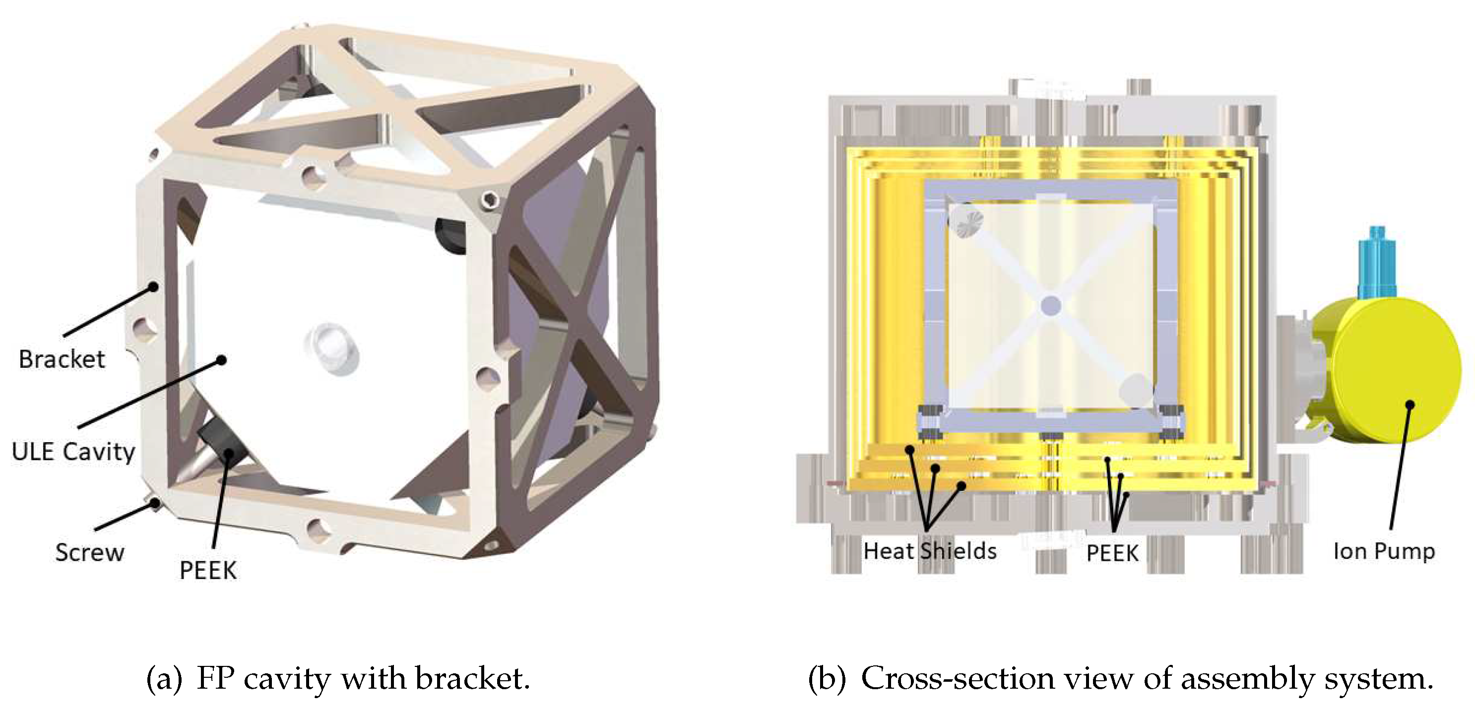
Figure 2.
displacement and Von Mises stress distributions.
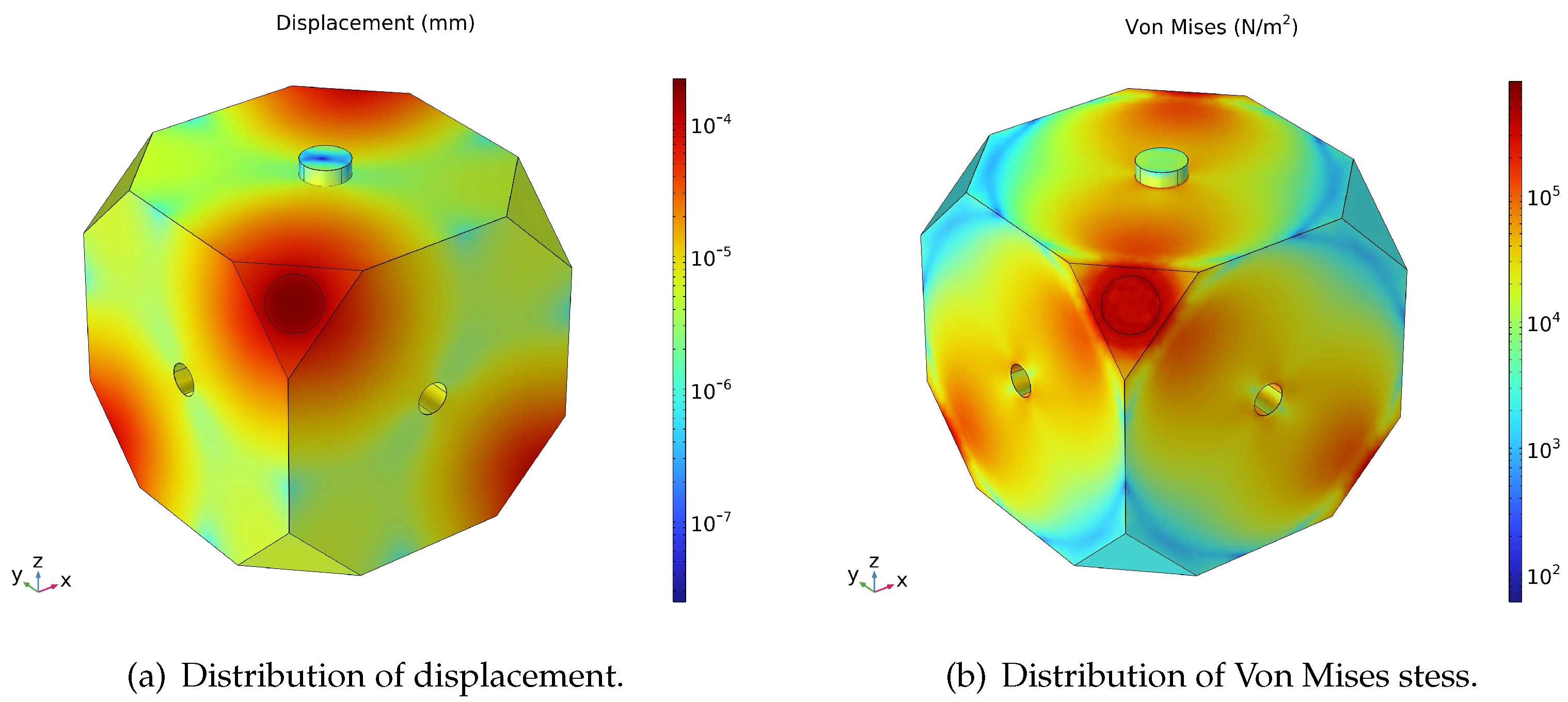
Figure 3.
Z component displacement of mirrors.
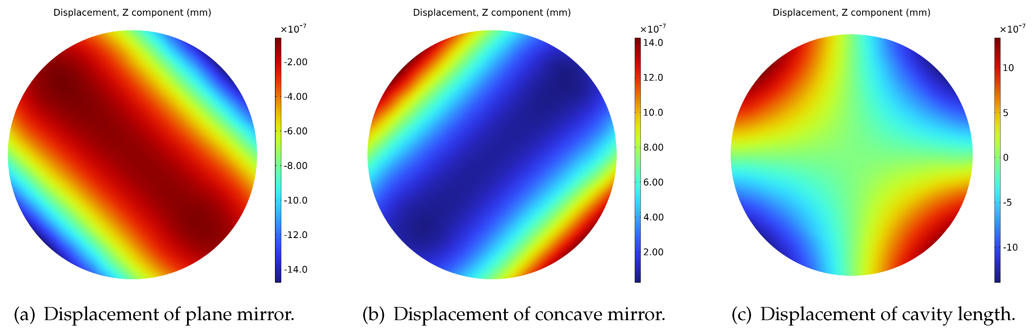
Figure 4.
EEMD results of cavity length change along and direction.
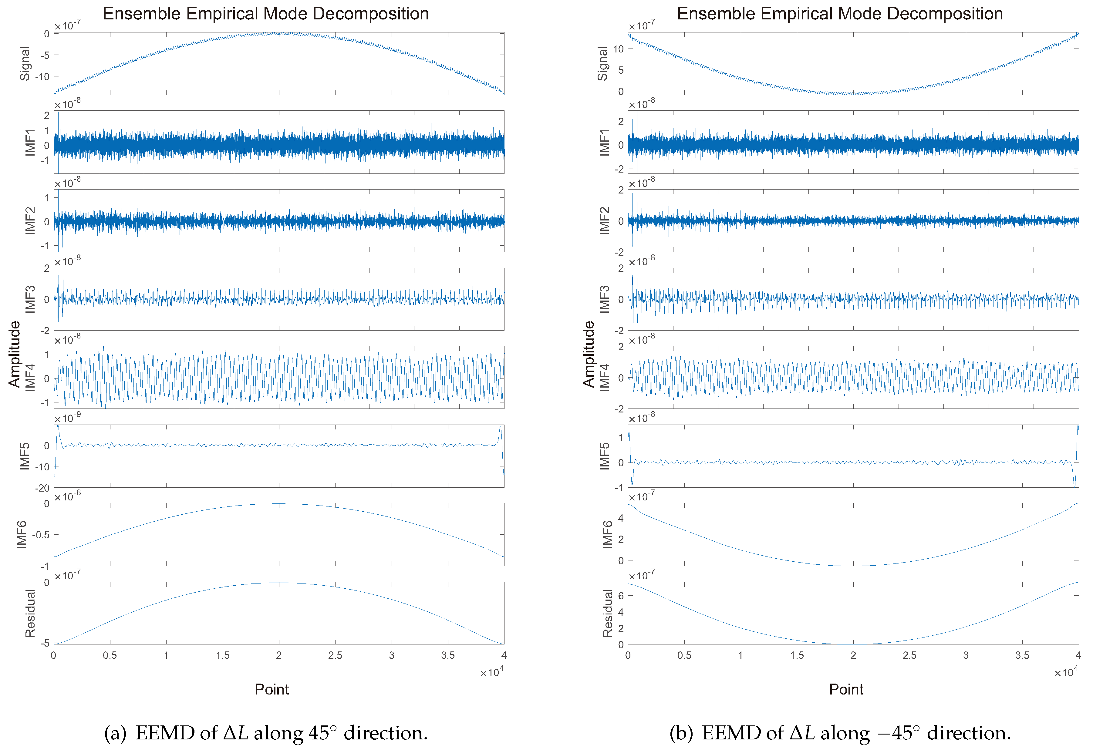
Figure 5.
Kurtogram of cavity length change along and direction.
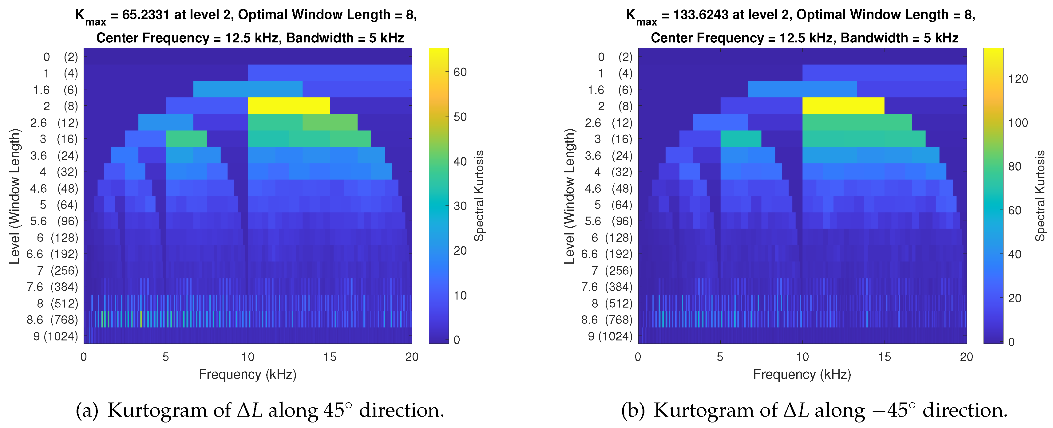
Figure 6.
Displacement Power spectrum density of cavity length change.
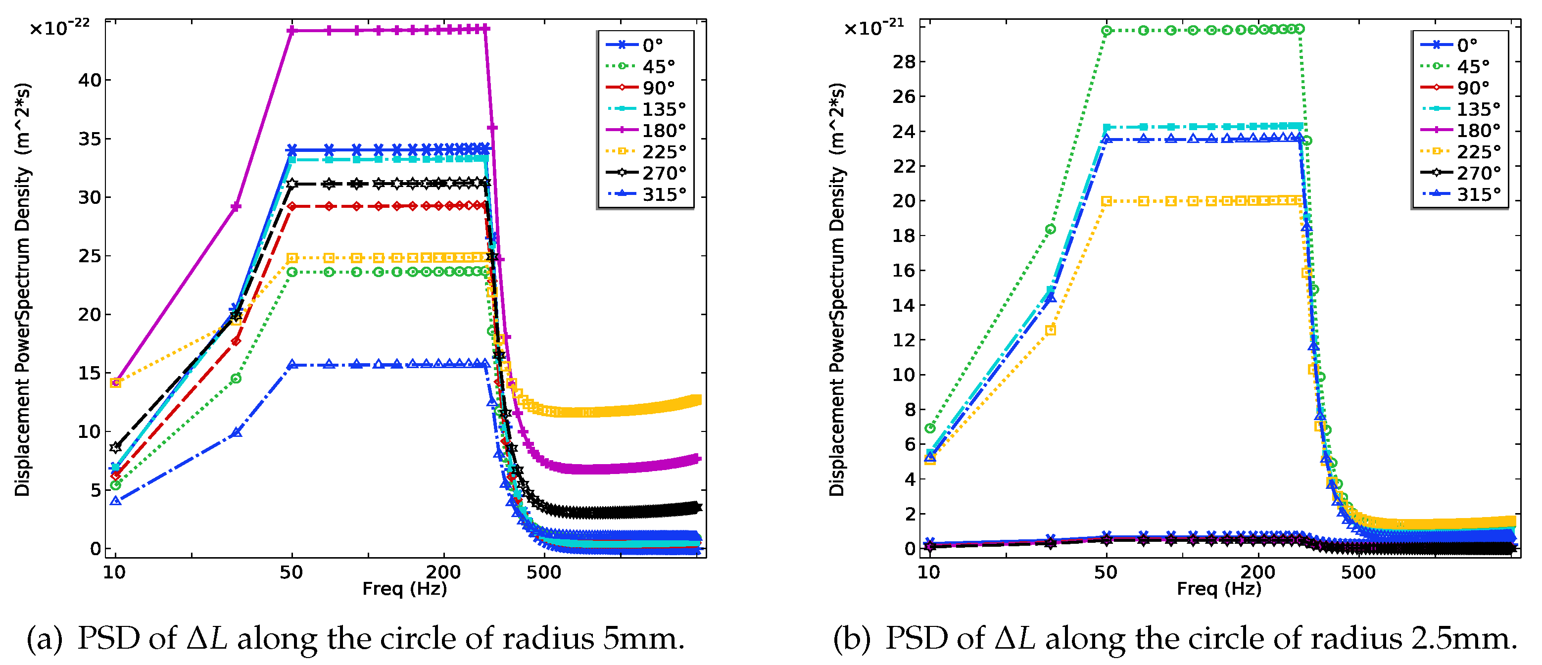
Figure 7.
displacement and Von Mises stress distributions at frequency 100 .

Figure 8.
Z component displacement of mirrors.
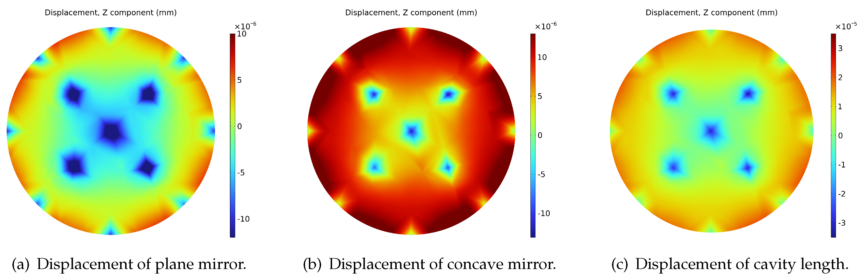
Figure 9.
EEMD results of cavity length change along and direction in vibration test.
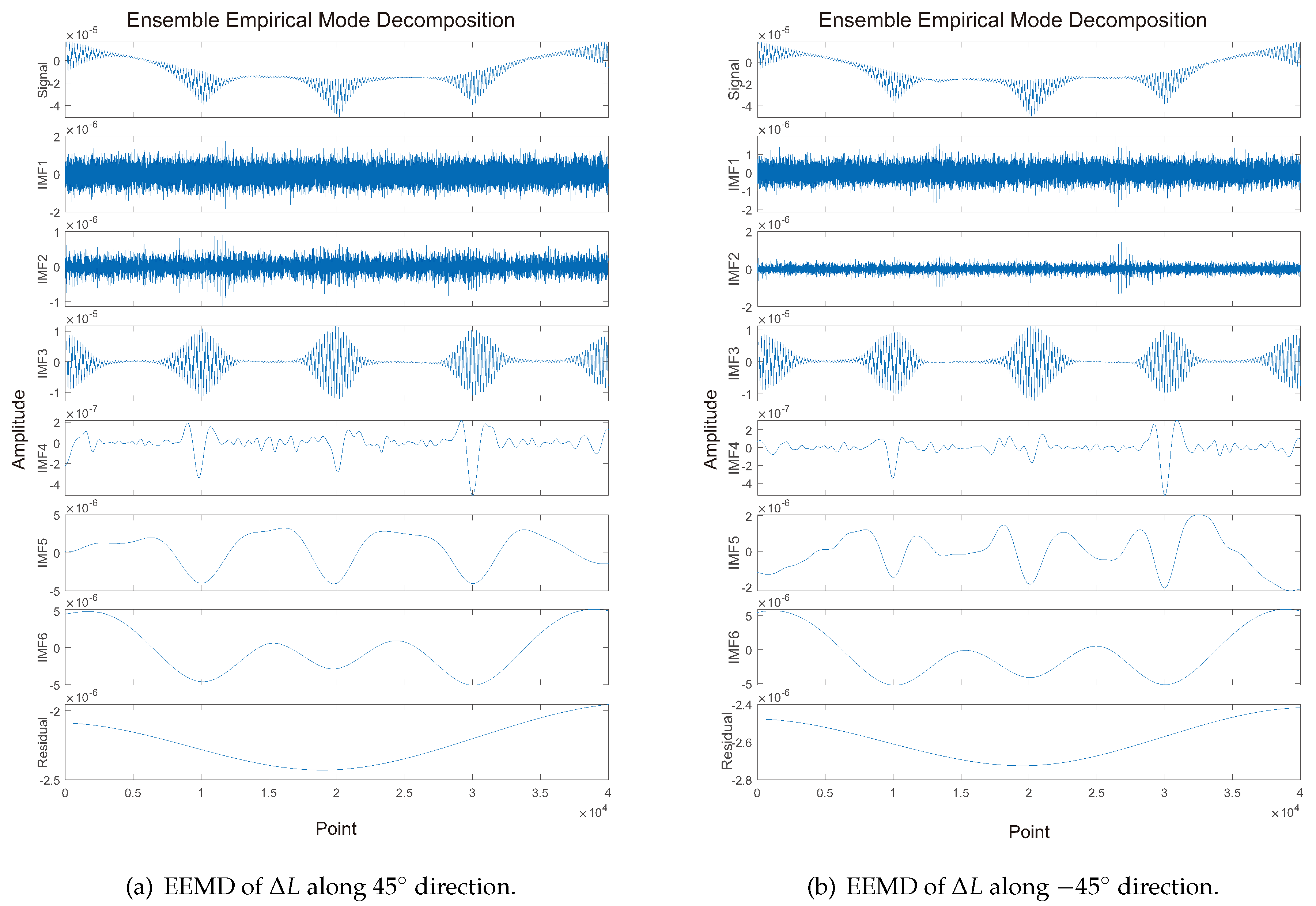
Figure 10.
Kurtogram of cavity length change along and direction under the vibration test.
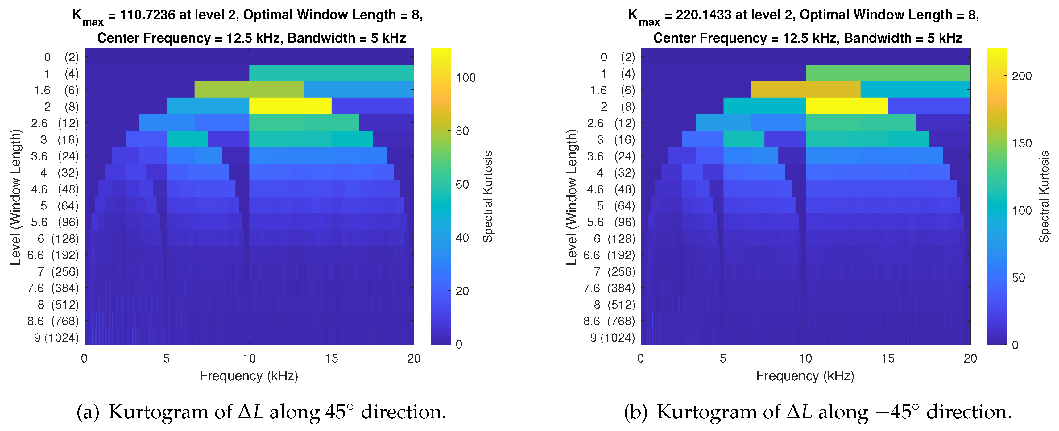
Figure 11.
Cavity design variables.
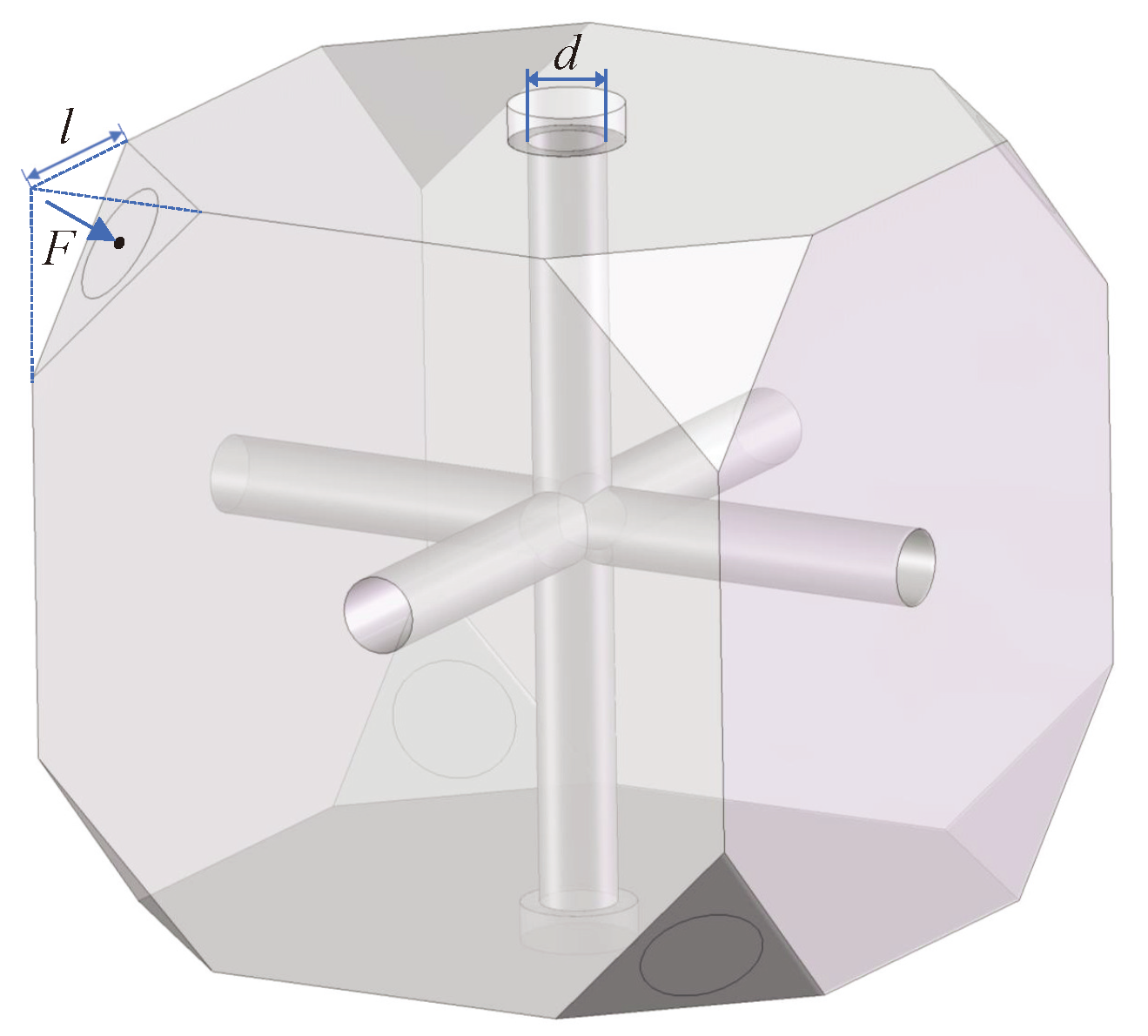
Figure 12.
Training results of neural network.
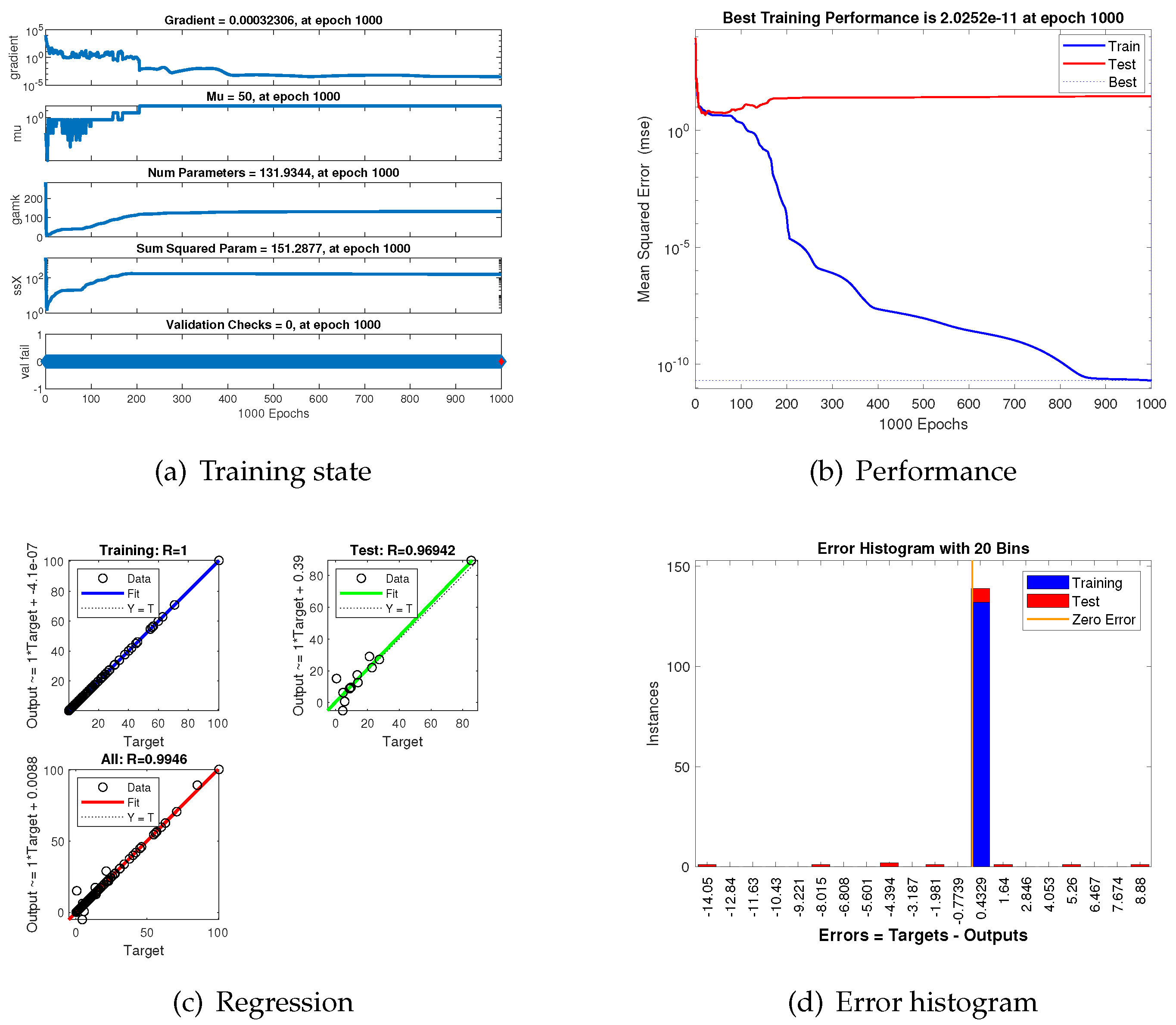
Figure 13.
prediction comparisons of Neural network and surrogate models.
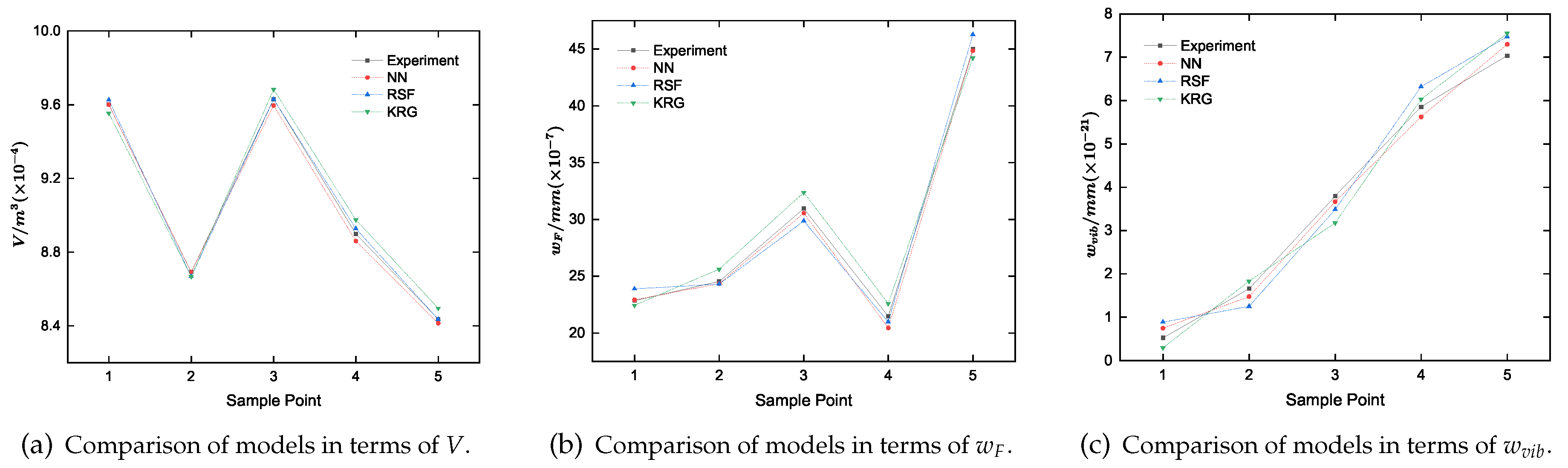
Figure 14.
Pareto Optimal Surface.
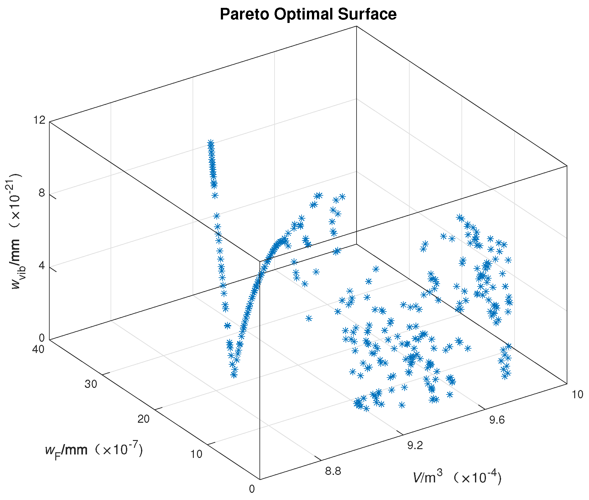

Table 1.
Parameters of the random vibration tests.
| Frequency Range / | Power Spectral Density |
|---|---|
| 10~50 | 3 (rising slope) |
| 50~300 | 0.25 (holding value) |
| 300~2000 | -12 (falling slope) |
Table 2.
Orthogonal experiment design and results.
| Number | d/mm | l/mm | F/N | () | () | () |
|---|---|---|---|---|---|---|
| 1 | 5 | 20 | 100 | 9.854 | 7.842 | 4.145 |
| 2 | 5 | 25 | 200 | 9.752 | 14.827 | 2.064 |
| 3 | 5 | 30 | 300 | 9.601 | 17.132 | 5.376 |
| 4 | 5 | 35 | 400 | 9.389 | 14.815 | 4.837 |
| 5 | 5 | 40 | 150 | 9.107 | 3.606 | 0.132 |
| 6 | 5 | 45 | 250 | 8.746 | 14.391 | 1.073 |
| 7 | 5 | 20 | 350 | 9.854 | 27.447 | 6.374 |
| 8 | 5 | 20 | 200 | 9.854 | 15.684 | 6.743 |
| 9 | 5 | 25 | 300 | 9.752 | 22.240 | 0.914 |
| 10 | 5 | 30 | 400 | 9.601 | 22.843 | 0.523 |
| 11 | 7 | 20 | 400 | 9.800 | 40.118 | 17.790 |
| 12 | 7 | 25 | 150 | 9.699 | 13.495 | 0.635 |
| 13 | 7 | 30 | 250 | 9.547 | 19.568 | 11.998 |
| 14 | 7 | 35 | 350 | 9.335 | 17.763 | 2.962 |
| 15 | 7 | 40 | 100 | 9.054 | 3.706 | 2.251 |
| 16 | 7 | 45 | 200 | 8.692 | 14.024 | 5.684 |
| 17 | 7 | 25 | 300 | 9.699 | 26.989 | 1.270 |
| 18 | 7 | 35 | 150 | 9.335 | 7.613 | 3.432 |
| 19 | 7 | 40 | 250 | 9.054 | 9.265 | 1.705 |
| 20 | 7 | 45 | 350 | 8.692 | 24.541 | 1.662 |
| 21 | 9 | 20 | 350 | 9.730 | 46.076 | 10.823 |
| 22 | 9 | 25 | 100 | 9.629 | 12.392 | 3.465 |
| 23 | 9 | 30 | 200 | 9.477 | 21.960 | 0.461 |
| 24 | 9 | 35 | 300 | 9.265 | 25.628 | 8.813 |
| 25 | 9 | 40 | 400 | 8.984 | 24.200 | 9.371 |
| 26 | 9 | 45 | 150 | 8.622 | 13.379 | 4.828 |
| 27 | 9 | 30 | 250 | 9.477 | 27.450 | 4.631 |
| 28 | 9 | 45 | 100 | 8.622 | 8.919 | 0.530 |
| 29 | 9 | 20 | 150 | 9.730 | 19.747 | 1.841 |
| 30 | 9 | 25 | 250 | 9.629 | 30.980 | 3.798 |
| 31 | 11 | 20 | 300 | 9.645 | 55.853 | 4.380 |
| 32 | 11 | 25 | 400 | 9.543 | 70.869 | 16.213 |
| 33 | 11 | 30 | 150 | 9.391 | 24.309 | 5.896 |
| 34 | 11 | 35 | 250 | 9.180 | 33.908 | 15.272 |
| 35 | 11 | 40 | 350 | 8.898 | 37.615 | 0.556 |
| 36 | 11 | 45 | 100 | 8.536 | 11.767 | 0.636 |
| 37 | 11 | 35 | 200 | 9.180 | 27.126 | 0.652 |
| 38 | 11 | 30 | 350 | 9.391 | 56.720 | 9.568 |
| 39 | 11 | 35 | 100 | 9.180 | 13.563 | 4.416 |
| 40 | 11 | 40 | 200 | 8.898 | 21.494 | 5.854 |
| 41 | 13 | 20 | 250 | 9.544 | 62.855 | 3.054 |
| 42 | 13 | 25 | 350 | 9.442 | 85.326 | 21.218 |
| 43 | 13 | 30 | 100 | 9.291 | 22.917 | 3.813 |
| 44 | 13 | 35 | 200 | 9.079 | 42.097 | 14.350 |
| 45 | 13 | 40 | 300 | 8.797 | 54.660 | 0.338 |
| 46 | 13 | 45 | 400 | 8.436 | 59.989 | 17.794 |
| 47 | 13 | 20 | 400 | 9.544 | 100.568 | 30.596 |
| 48 | 13 | 40 | 150 | 8.797 | 27.330 | 0.169 |
| 49 | 13 | 45 | 300 | 8.436 | 44.992 | 7.038 |
Table 3.
RMSE comparison of prediction models.
| Model | |||
|---|---|---|---|
| NN | 0.12 | 0.79 | 2.49 |
| RSF | 0.10 | 1.43 | 4.76 |
| KRG | 0.27 | 1.56 | 4.63 |
Table 4.
Performance comparison before and after optimization.
| d/mm | l/mm | F/N | ||||
|---|---|---|---|---|---|---|
| Before | 10 | 25 | 200 | 9.588 | 14.858 | 7.626 |
| After | 5 | 32 | 250 | 9.524 | 5.658 | 2.852 |
Disclaimer/Publisher’s Note: The statements, opinions and data contained in all publications are solely those of the individual author(s) and contributor(s) and not of MDPI and/or the editor(s). MDPI and/or the editor(s) disclaim responsibility for any injury to people or property resulting from any ideas, methods, instructions or products referred to in the content. |
© 2023 by the authors. Licensee MDPI, Basel, Switzerland. This article is an open access article distributed under the terms and conditions of the Creative Commons Attribution (CC BY) license (http://creativecommons.org/licenses/by/4.0/).
Copyright: This open access article is published under a Creative Commons CC BY 4.0 license, which permit the free download, distribution, and reuse, provided that the author and preprint are cited in any reuse.


