
Submitted:
14 November 2023
Posted:
15 November 2023
You are already at the latest version
Abstract
The linkage between the salt wedge, tidal patterns, and the Magdalena River discharge is established by assessing the ensuing parameters: stratification (ϵ), buoyancy frequency (β), potential energy anomaly (φ), Richardson number (RL), and bottom turbulent energy production (P). The salinity, temperature, density, and water velocity data utilized were derived from MOHID 3D, a previously tailored and validated model for the Magdalena River Estuary. To grasp the dynamics of the river, a flow regime analysis was conducted during both wet and dry climatic seasons of the Colombian Caribbean. The utilization of this model aimed to delineate the estuary's spatial reach, considering flow rates spanning from 2000 to 6500 m³/s across two tidal cycles. This approach facilitates the prediction of the position, stability, and stratification degree of the salt front. Among the conclusions drawn, it is highlighted that: 1. The river flow serves as the principal conditioning agent for the system, inducing a strong estuary response to weather stations; 2. The extent of wedge intrusion and the river discharge exhibit a non-linear, inversely correlation; 3. Tidal waves cause differences of up to 1000 m in the horizontal extent of the wedge; 4. Widespread channel erosion occurs during the rainy season when the salt intrusion does not exceed 2 km; 5. Flocculation processes intensify during the transition between dry and wet seasons; 6. The stability of the salt layering and the consolidation of the FSI-TMZ are contingent upon the geometric attributes of the channel.
Keywords:
Magdalena River Estuary
; Saline-Wedge Estuary
; Saline-Wedge Interannual Variability
; Discharge-salinity relationship
; Magdalena River Mouth Siltation.
1. Introduction
The circulation of water and sediment within estuaries is regulated by the density gradient between fresh and salt water [1]. These density variations give rise to a horizontal baroclinic gradient that strives to equalize the free surface level and the isopycnals [2]. As a result, a bidirectional water flow is initiated, commonly referred to as estuarine circulation. This process can be categorized based on whether the net volume outflow, which is associated with gravitational circulation exceeds or falls below the net volume inflow [3].
The interaction of river discharge, waves, currents, tidal patterns, and geomorphological factors collectively shapes the stratification and mixing dynamics of estuaries. In regions characterized by weak vertical stratification, such as tidal estuaries, the mixture of brackish water is uniform [4,5]. On the contrary, estuaries that are highly stratified encounter a constrained vertical mixing, resulting in the formation of a salt wedge [6,7]. Salt-wedge estuaries are frequently present at the mouths of microtidal coastal rivers, where the river outflow suppresses the effects of tidal mixing [8]. In this scenario, with an increasing river flow, the freshwater outflow prevails, forcing the denser saltwater downstream. In low discharge seasons, the tidal influx is amplified compared to the outflow, resulting in a greater depth of salt-wedge penetration upstream. This behavior highlights the river-controlled nature of most salt-wedge estuaries, which can either facilitate or impede the input of seawater [9,10,11,12]. It is important to emphasize the existence of tide-controlled estuaries that exhibit a time-dependent salt wedge development. The estuary of the São Francisco River in Northeast Brazil provides a suitable illustration [13].
Estuarine stratification is associated with the disruption of vertical transport mechanisms pertaining to nutrients and sediments, and it carries meaningful consequences for the productivity and functioning of these ecosystems [14,15]. Indeed, the salt wedge formation causes bottom anoxia (complete lack of oxygen) and hypoxia (low oxygen levels), negatively impacting benthic organisms [16]. The turbidity maximum zone (TMZ) is another essential factor in estuarine circulation. Positioned proximal to the upper boundary of the salt intrusion, this zone exhibits higher concentrations of finely suspended sediment when compared to those present in either the river or downstream areas of the estuary [17]. Intense flocculation processes occur in the TMZ, establishing a strong connection between the TMZ and estuarine siltation [18,19,20,21].
Fluvial estuaries, due to their location, have historically functioned as seaports and hubs for international trade. However, certain estuaries experience an increase in siltation rate that necessitates dredging channels to ensure and maintain ships navigability [22,23,24]. The Barranquilla seaport, located within the estuary of the Magdalena River (MRE), holds a vital role in the economy development of the city and its neighboring regions. This is mainly due to its distinction of having the largest number of terminals for international trade in Colombia [25,26]. Nonetheless, the seaport's operability encounters challenge due to the considerable difference between the maximum bed sedimentation rates (2625 mm/year) and the maximum erosion rates (1450 mm/year), which is almost a twofold magnitude difference [20]. Hence, in order to maintain a minimum draught of 10 meters, dredging operations are required [27]. The dredging procedure incurs high operational and logistical costs and does not offer a long-term solution. Moreover, it is conducted in disagreement with natural sedimentation patterns, rendering it an unsustainable approach [23,28].
The MRE is a microtidal saline-wedge conditioned by the river discharge [29,30]. Sedimentation mechanisms in the MRE are driven by the flocculation of suspended particles in the TMZ. The growth of the TMZ is correlated with the decrease in the bottom frictional energy of the water column during saline stratification, coupled with an increase in sediment availability. The decrease in bottom friction corresponds to the loss of the river's capacity for sediment resuspension, leading to the settling of flocs [31,32,33]. As previously noted, the displacement of the saline wedge is controlled by the energy of the Magdalena River. This results in heightened stratification during low discharge periods, when tidal and wave energy have a greater impact. Between 1997 and 1998, during the dry season of the warm phase of the El Niño Southern Oscillation (ENSO), it was estimated to have a maximum saltwater penetration of 20 kilometers upstream. Historical minimum flows, measuring around ~2000 m3/s, were recorded during this period. Conversely, during the wet season of the cold phase of the ENSO (between 1999 and 2000), the river outflow ranged from 10.000 m3/s to 14.000 m3/s, enclosing the salt-wedge extension to the first kilometer of the mouth [34].
A robust statistical correlation exists between the freshwater-saltwater interface (FSI) and the TMZ location [31]. Consequently, comprehending the dynamics of stratification not only provides valuable insights into the position of the FSI, but also facilitates inferences concerning the spatial localization of the TMZ [34]. Furthermore, studying the behavior of the saline-wedge can uncover opportunities to take advantage of the salinity gradient as a local energy source through the method of Reverse Electro-Dialysis (RED) [35,36]. All of this while not overlooking the ecological significance of FSI as an ecosystem rich in essential nutrients for vegetation and fauna [37,38,39]. This research aims to explore the effects of tidal patterns and seasonal fluctuations in river discharge on mixing dynamics, stratification, and the FSI’s spatial distribution as a predictive indicator of the TMZ’s formation. In this sense, our primary objective is to evaluate and delineate specific regions within the MRE where flocculation processes are expected to be intensified.
2. Study area
The MRE is located on the Caribbean coast of Colombia. It is formed by the confluence of the Magdalena River (MR) and the Caribbean Sea (CS). Due to its concentration of suspended sediment (CSS), it is classified as turbid and extremely turbid during high-flow seasons (CSS ≤ 11.450 mg/L) [31,39]. This phenomenon is primarily attributed to human intervention, the steep topographical features, and the substantial precipitation in the upper reaches of the MR basin, resulting in high erosion and sedimentation rates. Compared to other CS tributaries, the MR contributes the highest amount of suspended sediment (142.6 x10⁶ Tons/year) [40,41]. Globally, the MR is ranked as the seventh highest in sediment yield, surpassing well-known rivers such as the Amazon (190 Ton/Km2 year) or the Orinoco (140 Ton/Km2 year) [42]. Since the construction of the jetties in 1936 and subsequent modifications until 2009, the water flow velocity and sediment transport capability of the MR have increased [29,43]. This led to a gradual deepening of the MRE’s bed and cyclical changes between erosive (310 mm/year) and sedimentation (293 mm/year) states on interannual and intra-annual scales [20].
The climate exhibits two prevailing seasons: a wet season that lasts from May to December and a dry season that spans from January to April. These seasons are defined by the east-trade winds and the oscillation of the Intertropical Convergence Zone (ITCZ) [44,45]. On the MRE, winds have an average speed of 3.9 m/s, primarily blowing from the Northeast for 42.7% of the year and from the North for 25% of the year [29]. The significant wave height here is 2.2 ± 1.1 meters. It also originates from the Northeast and has an average period (T) of 6.7 ± 2.3 s. The maximum wave heights can reach up to 4.5 m during extreme weather events, such as the one that occurred in 2009, when a cold front caused the collapse of the Puerto Colombia pier [46]. The MRE has a mixed and semi-diurnal microtidal pattern based on the Courtier coefficient (1.43 ≤ F ≤ 1.9). Even during high tide, its tidal range does not exceed 70 cm in height [47,48,49]. The climate of the Colombian Caribbean Sea has a long-standing relationship with the El Niño Southern Oscillation (ENSO) in both of its phases, El Niño, and La Niña. The ENSO warm phase (El Niño) is associated with decreased precipitation and lower sea levels, while the ENSO cold phase (La Niña) is linked to higher sea levels and excessive rainfall [50,51,52].
3. Methodology
The assessment of stratification and mixing patterns in the MRE was conducted using a MOHID model that had been previously calibrated. This model considered multiple factors including bathymetry, river discharge, waves, and tides to simulate the estuary circulation as a function of the buoyancy gradient and bottom frictional stresses [29,30,34,53,54].
A total of twenty-six scenarios were analyzed under varying flow rates and tide conditions along a 22.0 km cross-section of the channel. To simulate the driving mechanism of tides, winds, and river flow, MOHID was implemented in a two-tiered nesting system (see Figure 1). The outer grid was configured to operate at a coarser resolution in barotropic mode with 220 x 250 nodes (Δx = Δy = 160 m y Δt = 10 s). The values for bottom roughness and horizontal turbulence were established as 0.0025 meters and 10 m2/s respectively. The inner grid was set to operate in baroclinic mode with 242 x 172 nodes operating at (Δx = Δy = 80 m y Δt = 5 s) and a vertical discretization of 48 layers using cartesian coordinates. This configuration enabled the simulation of localized sub-regions, such as the salt-wedge intrusion, while minimizing computational resource usage. The engaged flow rates ranged from 2000 to 6500 m3/s. Tidal simulations were conducted during both spring and neap states. However, to measure the overall tide effects in the salt-wedge position, the density and velocity water properties were averaged over two tidal cycles (25 hours) at a one-hour resolution (see Figure 2).
MOHID was developed by MARETEC, the Marine, Environment and Technology Center at the Technical University of Lisbon. It is a three-dimensional numerical model that simulates the response of water bodies to physical and biogeochemical processes, considering the interaction between water-atmosphere and water-sediments. MOHID was developed utilizing a block programming structure, which encompasses specialized modules to solve hydrodynamics, water quality, and particle tracking equations [55]. The MOHID Hydrodynamic module resolves the formulations of motion for incompressible and hydrostatically balanced fluids using the finite volume method and the Boussinesq and Reynolds approaches [56]. The system’s horizontal discretization employs an Arakawa-C-type computational grid [57], while the vertical axis enables the combination of Cartesian, Sigma, or Lagrangian coordinates. The implicit alternating direction algorithm is utilized to solve these equations, calculating the change in water elevation and velocities [58,59]. The vertical turbulence is inferred using the k-ϵ General Ocean Turbulence Model (GOTM) with the Canuto closure schemes [60]. For the horizontal turbulence, the Smagorinsky approach was employed with a coefficient value of 0.1. The selection was made based on its closeness to the measured data for both flow velocity and salinity (refer to Table 1). Finally, the horizontal and vertical advection and diffusion of momentum, heat, and mass were managed through implementation of the total variation diminishing method (TDV).
This model was calibrated with field measurements showing reliable and practical depictions of the MRE. Table 1 compares the Bias, RMSE, and Willmott coefficients [61] of the simulated and measured data for water salinity, velocity, and level performed during the dry season of February to March in 2018 and March 2020 [30]. The computed φ, β and RL values were based on field measurements during March of 2014 along the MRE [34].
It is a dimensionless measurement of the stratification intensity based on the density of the water column Here, the density gradient is represented by ∂ρ=ρ(bottom)- ρ(surface) and the average density is expressed as ρo=0.5 (ρb+ ρs). Usually, this parameter reaches values between 0 (indicating a well-mixed water plot) and 0.025 (indicating a highly stratified water plot).
3.1. Stratification and Mixing Parameters
To evaluate the strength of saline-wedge stratification in every scenario, several physical parameters were calculated, including Stratification (ϵ), Buoyancy Frequency (β), Potential Energy Anomaly (φ), Richardson Layered Number (RL), and Turbulence Production (P) (refer to Table 2).
3.2. Definition of the flow scenarios
Acknowledging the pivotal role of the MR discharge in the spatial position of the salt wedge [29,30], it is imperative to comprehend the seasonal probability distribution of this factor. Such comprehension will establish a connection between numerical modeling results and flow rate regimes. Based on daily field measurements from a limnimetric station located in the municipality of Calamar [66], the MR exhibits a strong monthly variability (see Table 3). Therefore, to assess its seasonal behavior, it was necessary to calculate the Empirical Cumulative Distribution Function (ECDF) [67]. This approach provides insights into the frequency and distribution of the MR outflow conditions.
The ECDF is a non-parametric estimator of the cumulative distribution function (CDF) based on the frequency of a given flow (x) relative to the total number of observations (n). It is a step function that only takes values in the range 0 to 1 and indicates the fraction of the data that is less than or equal to x [68]. The ECDF was applied to each series of daily flows per month, and then grouped by climatic stations (see Figure 3).
4. Results
Average monthly flow rate
The wet season includes the months related to the period of weak winds and high rainfall over the Colombian Caribbean. During this period, the flow of the RM reaches its highest levels of the year (~16900 m3/s). This is the opposite of the dry season, when the trade winds strengthen, bringing dry air from the Atlantic Ocean to the Caribbean. This event causes a decrease in the frequency and amount of precipitation, causing daily flows in the order of ~2500 m3/s.
During the transition from the wet to the dry season, the variability of flow reaches its peak in January and maintains a high level (Qmax / Qmin = 5.91) until February (refer to Table 3). This phenomenon is primarily due to the absence of rainfall between February and March at the river's estuary, coinciding with the Magdalena River basin's flushing and the ITCZ's positioning. It is evident that during these months, the probability distribution curve can be segmented into two distinct phases (see Figure 3B). An initial period of low slope and greater variability with flows between 4000-10000 m3/s achieved 50% of the time, followed by another high slope phase with discharges between 1500-4000 m3/s. This pattern confirms that the influence of the rainfall regime on the DDRM flow does not occur simultaneously.
Table 4 displays the accumulated probability of flows ranging from 2000 to 6500 m3/s. The table is sectioned by 500 m3/s increments, and the months with the greatest cumulative probability for each interval are outlined.
It is worth noting that flows ranging from 2000 to 3000 m3/s are considered uncommon occurrences. Even in March, the month with the highest likelihood of these ranges, their total magnitude does not exceed 24.31%. On the other hand, flows beyond 6500 m3/s occur 90.12% of the time in December, 95.48% in November and 85.65% in October. During the wet season, only scenarios with high flows have practical likelihoods. Conversely, in the dry season, there is more variability in flows that fall below 6500 m3/s. For instance, in February and March, flows ranging from 2000 to 5500 m3/s have a cumulative probability of 75.3% and 82.6%, respectively. These findings offer insight into the correlation between months when turbulent mixing is expected to decrease, for increase based on the river's seasonal flow.
Tidal effects on the stratification and penetration of the salt wedge
Figure 4 and Figure 5 depict the stratification parameters, buoyancy frequency, potential energy anomaly, and bottom turbulent kinetic energy production for the defined flow scenarios. In general, the vertical structure of the halocline and pycnocline follows a consistent pattern across tidal cycles, with notable variations for flows ranging from 5000 to 6500 m3/s. At syzygy tides, the stratification indices exceed 0.023 within the range of km 0 to 0.321 of the estuary. However, during the quadrature phase, only flows of 5000 and 5500 m3/s exhibit a value of ϵ ≥ 0.0226 between km 0 and 0.562. For flows of 6000 and 6500 m3/s, the stratification index is less than 0.083 in the distance interval between 0 and 0.562 kilometers. This indicates that tidal waves have a stronger impact on the vertical stratification of the ERM when the flow exceeds 5000 m3/s.
This is supported by analyzing the buoyancy coefficients and potential energy anomaly. Various methods are used to measure the degree of stratification in an estuary. Buoyancy refers to the inclination of a water column to rise or fall compared to an adjacent column due to differences in density, while the potential energy anomaly is the amount of energy required to mix a water column compared to the amount of energy required to mix the same quantity of water in a homogeneous column. Therefore, both indicators approach zero as stratification intensity decreases. Additionally, it should be noted that within the flow range of 5000 to 6500 m3/s, the buoyancy and potential energy anomaly reach their maximum values, albeit of lesser magnitude during quadrature as compared to syzygy. Moreover, it has been confirmed that the attenuation of these parameters is higher when the discharge values are 6000 and 6500 m3/s. For instance, at a distance of 560 meters inland, buoyancy changes from having a maximum value of β = 0.0132 s-2 during syzygy to a value of β = 0.0042 s-2 in quadrature. This finding establishes that the salt wedge's response to tidal cycles is not only apparent when the river flow surpasses 5000 m3/s, but it is also magnified between 6000 and 6500 m3/s. Furthermore, it has been discovered that the tide has an impact on the maximum intrusion penetration of CS, causing differences of up to 1000 meters. The most significant variations occur during discharges of 2500, 3500, 4250, 4500, 5500 and 6500 m3/s, as depicted in Figure 8.
Richardson number (as shown in Figure 6 and Figure 7) and bottom turbulent energy production (as seen in Figures 4D and 5D) are key indicators for assessing flow dynamics in relation to the stratification degree of the water column. Richardson reports that the fluid can maintain its stratification despite turbulent motions, while turbulent energy production signifies the amount of kinetic energy released into the water during turbulence. It has been observed that the maximum turbulence magnitudes are lower during syzygy tides along the entire section compared to those in quadrature. However, at low flow rates, the stability of the Richardson remains consistent. As the flow rate intensifies, bottom turbulence increases and causes mixing, thereby reducing the stability of the water parcel. As flow rate increases, it is argued that its ability to mix and hold particles in suspension also increases, thus limiting the precipitation of floccules.
Effects of flow rate on FSI position
According to [31] the location of the TMZ core is associated with the position of the FSI. The maximum depth of the FSI is recognized by the decrease in salinity and longitudinal density in the water column to its minimum, which is easily distinguishable in all stratification parameters.
FSI for flow rates from 2000 to 3000 m3/s
In this flow range, the position of FSI lies between km 14.3 and 21 of the section. There are distinct stratification levels between km 0 and 12, which are longitudinally maintained (ϵ ~ 0.026 y β ~ 0.019 s-2). Upstream, the gradual increase of mixing in the water column causes all parameters to decrease to their minimum values. At Q = 2000 m3/s, this happens from kilometer 20, while at Q = 3000 m3/s, it occurs from kilometer 12. For Q = 2500 m3/s, the location depends on the tidal stage: it happens at kilometer 17 during syzygy and at kilometer 17.5 during quadrature. Turbulent energy production at the riverbed is negligible (P ~ 0 W/Kg); resulting in underdeveloped mixing along the DDRM. In other words, greater levels of frictional strain are required to disrupt the stratification of CS. This is confirmed by Richardson number behavior (RL>20), which results in a stable column (stratified) due to the dominant buoyant force on turbulent bottom currents. At flow rates of Q = 2000 and 2500 m3/s, stability greatly increases (RL≫ 20) within the range of approximately km ~11.5 to ~17.5 due to the channel’s lateral widening. For a flow rate of Q = 2750 and 3000 m3/s, the potential energy anomaly φ concentrates energy in three locations where the maximum work required for water mixing is at approximately ~5.5, ~9 and ~12.5 kilometers. This is followed by two valleys at approximately ~7.5 and ~10.5 km. All locations have values of φ > 470 J/m3, which reaffirms the intense degree of stratification.
FSI for flow rates from 3250 to 4000 m3/s
The FSI spans from km 7.6 to 11.7. Throughout the initial section (km 0 - km 5), the indicators ϵ ~ 0.0275 y β ~ 0.0185 s-2 remain substantially unchanging. However, the stratification weakens beyond km 5 for Q = 4000 m3/s, km 6 (Q = 3500 m3/s), and km 9 (Q = 3250 m3/s) due to the increasing bottom turbulent production. At a Q = 4000 m3/s (located between km 6 - 13), the production is at ~ 3.45 x 10⁻⁵ W/Kg. At a Q = 3500 m3/s (located between km 9 - 13), the production is at P ~ 2.11 x 10⁻⁵ W/Kg. Lastly, at a Q = 3250 m3/s (located between km 10 - 13), it is the same as 2.11 x 10⁻⁵ W/Kg. The stability of the column, as anticipated, undergoes a decline when is at Q = 4000 m3/s whereby turbulent kinetic energy has a similar magnitude to hydrostatic potential energy. Specifically, RL acquires values between 2 and 20 explaining the weakening of the CS by the mixing strengthening. At Q = 3250 m3/s, the φ index initially rises from 565 J/m3 at km 0 to 1040.6 J/m3 at 5.4 km but subsequently declines as the stratification intensity increases.
FSI for flow rates from 4250 to 6500 m3/s
The FSI is between kilometers 1 and 6.5. Regarding the parameters, it is observed that at Q = 4250 m3/s, the maximum value of bottom turbulence is 4.30 x 10⁻⁵ W/Kg at km 11. At a Q = 4500 m3/s, the maximum turbulence (Pmax) is 5.29 x 10⁻⁵ W/Kg and is also achieved at kilometer 11. At a Q = 5000 m3/s the turbulent production starts at km 1.2 and equals two peaks: Pmax = 7.706 x 10⁻⁵ W/Kg (3.6 km) and Pmax = 7.68 x 10⁻⁵ W/Kg (11 km). At a Q = 5500 m3/s, β and φ suggest a decrease in stratification towards the Caribbean Sea during quadrature when comparing the maximum values in this phase (β = 0.0128 s-2) (φ = 636.18 J/m3) with the maximum values achieved during syzygy (β = 0.0151 s-2) (φ = 754.55 J/m3). For this flow rate, two peaks of turbulent production are reached: Pmax = 1.336 x 10⁻⁴ W/Kg (3.09 km) and Pmax = 1.05 x 10⁻⁴ W/Kg (11 km). At a Q = 6000 m3/s, the stratification index decreases from 0.02 (immediately at the estuary) to 2.65 x 10⁻³ in the first kilometer and in the quadrature phase. In syzygy, this decrease begins 560 m later. Indeed, between 0 - 560 m, ϵ approaches 0.0245. A similar trend is seen for β and φ at km 1, β = 0.0062 s-2 (syzygy) and β = 0.00145 s-2 (quadrature), which ensures that at this distance the tidal action has a stronger influence on the degree of stratification of the CS. In this scenario, mixing initiates at km 0 during quadrature, and km 0.25 in syzygy, which corresponds to two peaks of turbulent production. At a Q = 6500 m3/s, the magnitude of turbulent production is even higher and starts from km zero with two peaks: Pmax = 2.08 x 10⁻⁴ W/Kg (2.68 km) and Pmax = 1.32 x 10⁻⁴ W/Kg (11 km). Pmax = 2.80 x 10⁻⁴ W/Kg (2.52 km) and Pmax = 1.68 x 10⁻⁴ W/Kg (11 km).
5. Discussion
Tidal and flow effects on the salt wedge
The magnitude of flow rate and the extent of wedge intrusion displays a non-linear, inversely proportional relationship (as shown in Figure 8) described by the curve fitting formula: FSI (Q) = 1.133 x 10⁻⁶ Q2 – 0.0142 Q + 46.2825. The given regression model has a coefficient of determination (R2) of 0.9846, thereby reaffirming the river dominance in the MRE dynamics [29,30]. This model stands as a promising inaugural approximation for predicting the location of the FSI and, in extension, for delineating regions where the TMZ may consolidate [34]. Formerly, Zhang et al., 2010 undertook this endeavor within the Pearl River estuary. It is a microtidal-fluvial estuary distinguished by its shallow depth and funnel-shaped geometry. They applied two regression methodologies, yielding results in alignment with our own findings. There is a non-linear, inversely proportional bond between the salt intrusion length and the river's hydrodynamics. Furthermore, estuarine salinity exhibits variability not only due to the primary influence of the river but also in connection with the temporal alignment of peak flow events relative to the baseline flow conditions. These patterns have been observed in numerous estuaries worldwide, primarily through the application of Van der Burgh's coefficients [69,70,71].
It is important to recognize the limitations of this statistical fitting due to the role of tides in stratification and mixing in estuaries. Considering the same flow scenario, spring tides enhance salt layering. In contrast, during quadrature tides, mixing is increased, which implies less differentiation of layers in the water column. Based on the average impact of two tidal cycles, it was discovered that the intrusion depth can differ by up to 1 kilometer. However, if morphological changes in the channel are considered, this variation could increase exponentially. Research such as the one conducted by [72], indicates that dredging increases tidal inflow, a phenomenon yet to be studied within the context of MRE. This discovery provides new study perspectives in the short and medium term, including analysis throughout a complete tidal cycle, from high tide to low tide. Moreover, this factor has been shown to have a significant impact on estuarine circulation processes [29].
According to [31] the core of the TMZ is not only downstream of the FSI, but usually remains in close proximity to it, regardless of flow or tidal phase. This finding suggests that the TMZ can migrate along the MRE, similar to the FSI. Additionally, it was observed by [34] that TMZ intensifies with floc precipitation when the FSI penetrates into the countercurrent.
Flocs emerge as a consequence of the aggregation of colloidal particles [73]. Their dimensions are subject to sediment availability, organic matter concentration and estuarine hydrodynamics [74,75,76]. In the MRE, a significant amount of organic and inorganic material is present in suspension [33]. Consequently, the flocculation process is mainly conditioned by the frictional stresses in the bed, which depend mainly on the MR. The findings of this research indicate that the bottom turbulence production and the Richardson number can be used to infer the magnitude of the shear stress at the bottom τxy. Since P and τxy are directly proportional to each other, while RL y τxy are inversely related. The highest magnitude of shear stresses occurs when the river flow increases, particularly in two sections of the estuary, between kilometers 0-6 and 9-13.
Estuaries can be classified as partially mixed and salt wedge types based on their buoyancy coefficients (β). Partially mixed estuaries exhibit a β between 0.0025 and 0.01 s-2, while salt wedge estuaries have β values between 0.01 and 0.1 s-2 [62]. The findings obtained in this research confirm that the MRE can be classified into both categories depending on its tidal phase. During quadrature and syzygy, the MRE behaves as a salt wedge estuary for flows below 5500 and 6500 m3/s, respectively. This implies that for flows above these limits, its theoretical configuration corresponds to that of a partially mixed estuary. According to [34] this limit is set at 4000 m3/s, regardless of the tidal cycle.
FSI Monthly Mobility
Although the Magdalena River can reach flows as high as 17000 m3/s, analyzing its response to discharges below 6500 m3/s supplies sufficient insight into the dynamics of the salt wedge. It should be noted that it is in the lower flow scenarios that the greatest variability in the magnitude of the FSI occurs.
Table 5 is created by integrating the stratification-mixing indicators in the estuary with a statistical analysis of flow regimes. It displays the monthly ranges where the FSI and TMZ are mobilized by proximity. For all instances, the cumulative probability (Pa) helps to validate the feasibility of each interval in both Neap Tide (NT) and Spring Tide (ST). In this sense, it can be stated that 90.1% of the time the flows between 6000 and 14583 m3/s occur in December, which means that the FSI is unable to penetrate beyond 2.2 km, regardless of the tidal cycle. During this month, its lowest intrusion depth is estimated, and the highest turbulent production rate occurs at the bottom of the estuary. As for January, the RM discharge begins to decline, which results in a greater stratification and deepening of the CS up to a maximum of 14.2 km. Approximately, this should be located around km 7.1 ± 7.1.
During February, the CS gradually moves upstream, from oscillating around km 9.7 ± 9.7 to stopping above km 11 ± 10 in March, at which point it is expected to reach its maximum extent before receding due to increased river flow. By April, it is found above km 9.7 ± 9.7, above km 4.5 ± 4.5 in May, and at 1.8 ± 1.8 km in June. It advances against the current again for both July and August, stopping in both cases near km 5.8 ± 5.8. In September, the halocline is located at approximately km 4.5 ± 4.5 and retreats in October (km 1.8 ± 1.8), November (km 1.4 ± 1.4), and December (km 1.2 ± 1). This pattern suggests that the FSI positioning is highly responsive to changes in intra-annual scales and consistently remains focused around km 5.
Considering that accelerated floc precipitation occurs when turbulent stratification is disrupted, it can be argued that an increase in bed sedimentation is promoted during the initial phase of the dry-rainy climate transition. Two important processes take place during this phase. First, the capacity of the RM to transport larger fragments increases. Second, the FSI-TMZ emerges from the stream, which favors sediment uptake. Specifically, it follows that during the most intense transition of the year (February-March-April), the precipitation volume peaks between km 1 and 9.7 ± 9.7. Furthermore, it is expected that the periods of greatest erosion in the MRE are associated with the restriction of the CS above km 2, due to the increase in Q and the intensification of bottom shear.
Probabilistic Model Validation
Although the FSI-TMZ relationship proposed here is based on the characterization of the mean RM regime and the application of a previously calibrated and validated numerical model, it is evident that estuarine circulation processes involve complex interactions that are difficult to synthesize using such approaches [7]. For this reason, a case study is presented that integrates the probabilistic flow regime (refer to Figure 9) and a multi-bathymetric analysis of the bed for the year 2016.
Ref. [20] found that sedimentation processes were dominant during the transitions between March-February and August-July in the MRE, with an average rate of 883 mm/m (March-February) and 271 mm/m (August-July). Moreover, the data collected showed that a maximum accumulation of 8628 mm/m was recorded above kilometer 4.5 specifically in the August-July transition period. Similarly, the study discovered that the erosion processes with the highest intensity take place during the transitions of February-January, September-August, October-September, November-October, and December-November, as well as in close proximity to kilometer 4.5. The average scour rate ranged from 194 mm/m (October-September) to 952 mm/m (February-January) with a maximum of 13222 mm/m in December-November. In April-March, May-April, June-May, and July-June, a mixed range was identified with a slight predominance of erosional processes. The range in average erosion and accommodation rates is 112-835 mm/m and 165-833 mm/m, respectively. However, there are spatial differences in the distribution of these processes. For instance, the most significant sedimentation processes occur between km 0-3 on the western margin (May-April), 0-3 km on the eastern margin (July-June), 0-2 km (June-May) and km 5 (April-March).
According to the functional model presented in this research (refer to Table 6), the salt wedge can migrate up to a maximum of 20.2 km and 5.5 km in March-February and August-July, respectively. During the first period, there was a retreat observed from ~20 km (February) to ~17.5 km (March). This movement occurred due to a rise in mean flow magnitude of 200 m3/s (February: 2467 m3/s, March: 2681 m3/s) that resulted in the accumulation of particulate material without disrupting channel stratification. During the second period, there is a comparable occurrence where the average flow increases from 5268 m3/s (July) to 5323 m3/s (August) with a maximum FSI amplitude of 3.6 km (July) and 5.5 km (August). Note that the average sedimentation rate in March-February is more than three times higher than in August-July, and that turbulent energy production is practically nil for flows between 2500 and 3000 m3/s (March-February). This is different from the production related to discharges in the order of 5000 m3/s (August-July), which has two energy maxima: at kilometer 3 (Pmax = 1.336 x 10⁻⁴ W/Kg) and at kilometer 11 (Pmax = 1.05 x 10⁻⁴ W/Kg). As mentioned, higher shear stresses on the bed promote resuspension and aggregation of material, while hindering its sedimentation. This is why the precipitated volume during March-February is much higher, and sedimentation in August-July is focused between kilometers 3 and 11. In this section, turbulent energy decreases substantially, which causes the deposition of the previously accreted flocs that remained in suspension (as seen in Figure 4D and Figure 5D).
During the analysis of intervals featuring the most significant erosion, it was found that a correlation exists with the periods when the wedge is constricted towards the river's estuary. Specifically, this correlation is noticeable at km 2.7 ± 0.8 in September and 3.5 ± 1.5 in August, and during the October-September period (km 1.4±0.5 and km 2.5 ± 0.9), November-October (km ~0 and km 1.4±0.5), and December-November (km ~0). However, an anomaly occurs during the February-January period. Although the FSI-TMZ is capable of penetrating to a depth of approximately (~20.2 km), the river experiences a decrease in competence during this stage, with the mean flow dropping from 2706 m3/s to 2467 m3/s. As a result of this reduction in flow, suspended material is precipitated and moves towards the front of the CS.
6. Conclusions
Numerical modeling is a versatile and effective tool for predicting the behavior of the salt wedge in the Magdalena River under various scenarios. This facilitates the development of planning processes such as risk management, energy utilization of the saline gradient, and programming of dredging activities. Both the numerical model and the probabilistic scheme have proven to be valuable tools in the representation and prediction of stratification and estuarine mixing processes.
The findings of this research show the complex interconnection between river flow, the extent of intrusion, and the degree of salt wedge stratification. In particular, flow was identified as the main conditioning agent of the system. Therefore, the behavior of the ERM responds strongly to seasonal scales, as the flow is linked to the rainfall regime, and both the stratification and the horizontal extent of the FSI decrease as the water flow increases. Furthermore, the importance of tidal waves in the differentiation of layers and the degree of penetration of the FSI has been found. Significant variations of up to 1000 meters have been observed in the extent and vertical structure configuration of the estuary, particularly during instances when river flow exceeds specific thresholds. These findings are crucial in comprehending the dynamics of the estuary involving sedimentation and bed erosion. In particular, it is noted that during the transitions between dry and wet seasons, the volume of sediment deposited reaches its annual maximum. For most of the year, it is expected that the FSI will be located beyond kilometer 5, with a maximum range of 11 ± 10 km. However, the most significant erosion processes will likely occur between kilometers 3 and 11, during the months when the CS is restricted to kilometer 2, leading to an increase in turbulent bottom production that limits floc settlement.
Finally, it is important to emphasize that the geometric configuration of the river plays a fundamental role in the stability of the water column. Indicators such as the Richardson number allow us to affirm that a widening of the channel strengthens the stability of the stratification in both syzygy and quadrature tides. In fact, the influence of this geometrical effect is stronger than the average variations between different tidal phases as this parameter shows no significant changes between stages. This conclusion is particularly relevant to the dredging operations frequently undertaken in the Magdalena River estuary
Author Contributions
Formal analysis, Jhonathan Cordero-Acosta; Investigation, Jhonathan Cordero-Acosta; Methodology, Luis Otero Díaz; Software, Aldemar Higgins Álvarez; Supervision, Luis Otero Díaz; Writing – original draft, Jhonathan Cordero-Acosta; Writing – review & editing, Luis Otero Díaz and Aldemar Higgins Álvarez.
Funding
This research received no external funding.
Conflicts of Interest
The authors declare no conflict of interest.
References
- Pritchard, DW. Estuarine circulation patterns. Proc Am Soc Civil Eng. 1955;81(717):1–11.
- Geyer WR, MacCready P. The Estuarine Circulation. Annu Rev Fluid Mech. 2014;46(1):175–97.
- Valle-Levinson, A. 1.05 - Classification of Estuarine Circulation. In: Wolanski E, McLusky D, editors. Treatise on Estuarine and Coastal Science. 2011. p. 75–86.
- Haas, LW. The effect of the spring-neap tidal cycle on the vertical salinity structure of the James, York and Rappahannock Rivers, Virginia, U.S.A. Estuarine and Coastal Marine Science. 1977;5(4):485–96.
- Dyer KR, New AL. INTERMITTENCY IN ESTUARINE MIXING. In: Wolfe DA, editor. Estuarine Variability. 1986. p. 321–39.
- Valle-Levinson, A. Contemporary Issues in Estuarine Physics. Valle-Levinson A, editor. Cambridge: Cambridge University Press; 2010.
- MacCready P, Geyer WR. Advances in estuarine physics. Annu Rev Mar Sci. 2010;2:35–58.
- Hansen D V, Rattray Jr M. NEW DIMENSIONS IN ESTUARY CLASSIFICATION1. Limnol Oceanogr. 1966;11(3):319–26.
- Perales-Valdivia H, Sanay-González R, Valle-Levinson A. Effects of tides, wind, and river discharge on the salt intrusion in a microtidal tropical estuary. Reg Stud Mar Sci. 2018;24:400–10.
- Zachopoulos K, Kokkos N, Sylaios G. Salt wedge intrusion modeling along the lower reaches of a Mediterranean river. Reg Stud Mar Sci. 2020;39:101467.
- Couceiro MAA, Schettini CAF, Siegle E. Modeling an arrested salt-wedge estuary subjected to variable river flow. Reg Stud Mar Sci. 2021;47:101993.
- Krvavica N, Gotovac H, Lončar G. Salt-wedge dynamics in microtidal Neretva River estuary. Reg Stud Mar Sci. 2021;43:101713.
- Paiva BP, Schettini CAF. Circulation and transport processes in a tidally forced salt-wedge estuary: The São Francisco river estuary, Northeast Brazil. Reg Stud Mar Sci. 2021;41:101602.
- Uncles R, Ong J, Gong W. Observations and analysis of a stratification destratification event in a tropical estuary. Estuar Coast Shelf Sci. 1990;31:651–65.
- Newton A, Icely J, Cristina S, Brito A, Cardoso AC, Colijn F, et al. An overview of ecological status, vulnerability, and future perspectives of European large shallow, semi-enclosed coastal systems, lagoons, and transitional waters. Estuar Coast Shelf Sci. 2014;140:95–122.
- Huang P, Kilminster K, Larsen S, Hipsey MR. Assessing artificial oxygenation in a riverine salt-wedge estuary with a three-dimensional finite-volume model. Ecol Eng. 2018;118:111–25.
- Dyer, K. Estuarine Circulation. In: Steele JH, editor. Encyclopedia of Ocean Sciences. 2001. p. 846–52.
- Guo L, He Q. Freshwater flocculation of suspended sediments in the Yangtze River, China. Ocean Dyn. 2011;61(2–3, SI):371–86.
- Silva-Dias FJ, Castro BM, Lacerda LD, Miranda LB, Marins R V. Physical characteristics and discharges of suspended particulate matter at the continent-ocean interface in an estuary located in a semiarid region in northeastern Brazil. Estuar Coast Shelf Sci. 2016;180:258–74.
- Restrepo JC, Orejarena A, Consuegra C, Pérez J, Llinas H, Otero L, et al. Siltation on a highly regulated estuarine system: The Magdalena River mouth case (Northwestern South America. Estuar Coast Shelf Sci. 2020;245:272–7714.
- Ming Y, Gao L. Flocculation of suspended particles during estuarine mixing in the Changjiang estuary-East China Sea. Journal of Marine Systems. 2022;233:103766.
- Geyer WR, Woodruff JD, Traykovski P. Sediment transport and trapping in the Hudson River estuary. Estuaries. 2001;24(5):670–9.
- Li M, Ge J, Kappenberg J, Much D, Nino O, Chen Z. Morphodynamic processes of the Elbe River estuary, Germany: the Coriolis effect, tidal asymmetry and human dredging. Front Earth Sci. 2014;8(2):181–9.
- Orseau S, Huybrechts N, Tassi P, Bang D, Klein F. Two-dimensional modeling of fine sediment transport with mixed sediment and consolidation: Application to the Gironde Estuary, France. International Journal of Sediment Research. 2021;36(6):736–46.
- Urbano Latorre CP, Otero Díaz LJ, Lonin S. Influencia de las corrientes en los campos de oleaje en el área de Bocas de Ceniza, Caribe Colombiano. Boletín Científico CIOH [Internet]. 2013;31:191–206. [CrossRef]
- Assessment, LC. 2.1.2 Colombia Port of Barranquilla [Internet]. 2021. Available from: https://dlca.logcluster.org/x/8oJv.
- MIN.TRANSPORTE. Cormagdalena y Findeter garantizan dragado en el río Magdalena en el 2021 gracias a la suscripción del contrato interadministrativo. Sitio web nacional Ministerio de Transporte Publicación [Internet]. 2020;9296. Available from: https://www.mintransporte.gov.co/publicaciones/9296/cormagdalena-y-findeter-garantizan-dragado-en-el-rio-magdalena-en-el-2021-gracias-a-la-suscripcion-del-contrato-interadministrativo/.
- Jang D, Hwang J, Park Y, Park S. A study on salt wedge and River Plume in the Seom-Jin River and estuary. KSCE Journal of Civil Engineering. 2012;16:10 1007 12205–012–1521–9.
- Ospino S, Restrepo JC, Otero L, Pierini J, Alvarez-Silva O. Saltwater intrusion into a river with high fluvial discharge: A microtidal estuary of the Magdalena River, Colombia. J Coast Res. 2018;34(6):1273–88.
- Higgins A, Otero L, Restrepo JC, Álvarez O. The effect of waves in hydrodynamics, stratification, and salt wedge intrusion in a microtidal estuary. Front Mar Sci. 2022;2296–7745.
- Restrepo JC, Schrottke K, Traini C, Bartholomae A, Ospino S, Ortíz JC, et al. Estuarine and sediment dynamics in a microtidal tropical estuary of high fluvial discharge: Magdalena River (Colombia, south america. Mar Geol. 2018;398:86–98.
- Arevalo FM, Álvarez-Silva Ó, Caceres-Euse A, Cardona Y. Mixing mechanisms at the strongly-stratified Magdalena River’s estuary and plume. Estuar Coast Shelf Sci. 2022;277:108077.
- Restrepo JC, Ospino O, Torregroza-Espinosa AC, Ospino S, Villanueva E, Molano-Mendoza JC, et al. Variability of suspended sediment properties in the saline front of the highly stratified Magdalena River estuary, Colombia. Journal of Marine Systems. 2024;241:103894.
- Otero L, Hernández H, Higgins A, Restrepo JC, Álvarez O. Interannual and seasonal variability of stratification and mixing in a high-discharge micro-tidal delta: Magdalena River, Colombia. Journal of Marine Systems [Internet]. 2021;224:103621. [CrossRef]
- Álvarez O, Osorio A. Salinity gradient energy potential in Colombia considering site specific constraints, Colombia. Renew Energy [Internet]. 2015;74:737 – 748. [CrossRef]
- Roldan M, Vallejo S, Álvarez O, Bernal S, Arango S, Sánchez C, et al. Salinity gradient power by reverse electrodialysis: A multidisciplinary assessment in the Colombian context. Desalination. 2021;503:11–9164.
- Sheppard, C. The Estuarine Ecosystem: Ecology, Threats and Management, Third Edition. Mar Pollut Bull [Internet]. 2004;49:9–10. [CrossRef]
- Statham, PJ. Nutrients in estuaries — An overview and the potential impacts of climate change. Science of The Total Environment [Internet]. 2012;434:213–27. [CrossRef]
- Torregroza, AC. Spatio-temporal distribution of temperature, salinity, and suspended sediment on the deltaic front of the Magdalena River: Influence on nutrient concentration and primary productivity. Journal Article, Salinity and Marine Sediments. 2020. [Google Scholar]
- Higgins A, Restrepo JC, Ortíz J, Pierini J, Otero L. Suspended Sediment Transport in the Magdalena River (Colombia, South America): Hydrologic Regime, Rating Parameters and Effective Discharge Variability. International Journal of Sediment Research. 2015;31:10 1016 2015 04 003.
- Restrepo JC, Ortíz J, Otero L, Ospino S. Transporte de sedimentos en suspensión en los principales ríos del Caribe colombiano: magnitud, tendencias y variabilidad. Rev Acad Colomb Cienc Exactas Fis Nat. 2015;39:527–46.
- Milliman J, Farnsworth K. River Discharge to the Coastal Ocean: A Global Synthesis. Cambridge: Cambridge University Press; 2011.
- Restrepo JC, Schrottke K, Traini C, Ortíz JC, Rondón A, Otero L, et al. Sediment Transport Regime and Geomorphological Change in a High Discharge Tropical Delta (Magdalena River, Colombia): Insights from a Period of Intense Change and Human Intervention (1990-2010. J Coast Res. 2015;32:10 2112 – 14–00263 1.
- Pérez-Santos I, Schneider W, Sobarzo M, Montoya-Sánchez R, Valle-Levinson A, Garcés-Vargas J. Surface wind variability and its implications for the Yucatan basin-Caribbean Sea dynamics. J Geophys Res. 2010;115:10052.
- Ruiz, OM. Variabilidad de la Cuenca Colombia (mar Caribe) asociada con El Niño-Oscilación del Sur, vientos Alisios y procesos locales. Deoartamento de Geociencias y Medio Ambiente, UNAL [Internet]. 2011; Available from: https://repositorio.unal.edu.co/handle/unal/8181.
- Ortiz J, Otero L, Restrepo JC, Ruiz J, Cadena M. Characterization of cold fronts in the Colombian Caribbean and their relationship to extreme wave events. Nat Hazards Earth Syst Sci. 2013;13:2797–804.
- Molares, BR. Clasificación e identificación de las componentes de marea del Caribe colombiano. Boletín Científico CIOH. 2004;24:105–14.
- Restrepo JD, López SA. Morphodynamics of the Pacific and Caribbean deltas of Colombia, South America. J S Am Earth Sci. 2008;25:1–21.
- Pérez, R. A, Ortiz R. JC, Bejarano A. LF, Otero D. L, Restrepo L. JC, Franco H. A. Sea breeze in the Colombian Caribbean coast. Atmósfera [Internet]. 2018;31(4):389–406. [CrossRef]
- Bedoya-Soto JM, Poveda G, Trenberth KE, Vélez-Upegui JJ. Interannual hydroclimatic variability and the 2009–2011 extreme ENSO phases in Colombia: From Andean glaciers to Caribbean lowlands. Theor Appl Climatol. 2019;135:1531–44.
- Cai W, McPhaden M, Grimm A, Rodrigues R, Taschetto A, Garreaud R, et al. Climate impacts of the El Niño–Southern Oscillation on South America. Nat Rev Earth Environ. 2020;1:215–31.
- Vega MJ, Alvarez-Silva O, Restrepo JC, Ortiz JC, Otero LJ. Interannual variability of wave climate in the Caribbean Sea. Ocean Dyn. 2020;70(7):965–76.
- Higgins A, Otero L, Restrepo JC, Álvarez O. Variabilidad estacional de la interacción oleaje-corriente y dinámica de la cuña salina en la desembocadura del Delta del río Magdalena. In: I.N.V.E.M.A.R.-A.C.I.M.A.R., editor. Libro de resúmenes extendidos XVI Senalmar. 2017. p. 76–80.
- Higgins A, Restrepo JC, Otero L, Ortiz JC, Conde M. Vertical distribution of suspended sediment in the mouth area of the Magdalena River, Colombia. Lat Am J Aquat Res. 2017;45:724–36.
- MARETEC. MOHID WATER [Internet]. MOHID OFFICIAL WEBPAGE. 2020. Available from: http://www.mohid.com/pages/models/mohidwater/mohid_water_home.shtml.
- Martins F, Neves R, Leitao P, Silva A. 3D modeling in the Sado estuary using a new generic vertical discretization approach. Oceanol Acta. 2001;24:51–62.
- Arakawa. Computational design for long-term numerical integration of the equations of fluid motion: two-dimensional incompressible flow. Part I J Comput Phys. 1966;1:119–43.
- Leendertse, JJ. Aspects of a Computational Model for Long-period Water-wave Propagation. Santa Monica, CA: RAND Corporation; 1967.
- Abbott MB, Damsgaard A, Rodenhuis GS. System 21, Jupiter, a design system for two-dimensional nearly horizontal flows. J Hydraul Res. 1973;11:1–28.
- Canuto VM, Howard A, Cheng Y, Dubovikov MS. Ocean turbulence I: One-point closure model—Momentum and heat vertical diffusivities. J Phys Oceanogr. 2001;31:1413–26.
- Willmott C, Ackleson S, Davis R, Feddema J, Klink K, Legates D, et al. Statistics for the evaluation and comparison of models. J Geophys Res Oceans. 1985;90(C5):8995–9005.
- Geyer WR, Scully ME, Ralston DK. Quantifying vertical mixing in estuaries. Environmental fluid mechanics. 2008;8(5):495–509.
- Simpson J, Crisp D, Hearn C. The shelf-sea fronts: implications of their existence and behaviour [and discussion]. Lond A. 1981;302:531–46.
- MacKay H, Schumann E. Mixing and circulation in the Sundays River estuary, South Africa. Estuar Coast Shelf Sci. 1990;31:203–16.
- Ralston DK, Geyer WR, Lerczak JA, Scully M. Turbulent mixing in a strongly forced salt wedge estuary. J Geophys Res Oceans. 2010;115:12024.
- IDEAM. Serie de caudal medio diario. Periodo 23/07/1940 y 31/12/2015. Estación limnimétrica CALAMAR [29037020]. Departamento de Bolívar, Municipio Calamar [Internet]. Available from: http://dhime.ideam.gov.co/atencionciudadano/.
- Pernot P, Savin A. Probabilistic performance estimators for computational chemistry methods: the empirical cumulative distribution function of absolute errors [Internet]. 2018. [CrossRef]
- Wischik, D. Foundations of Data Science [Internet]. University of Cambridge; 2020. Available from: https://www.youtube.com/watch?v=JrS1ajLqMZQ&list=PLknxdt7zG11O5BV8ipHD30dnupEk-tKjn&index=24.
- Gisen JIA, Savenije HHG, Nijzink RC. Revised predictive equations for salt intrusion modelling in estuaries, Hydrol. Earth Syst Sci [Internet]. 2015;19:2791–803. [CrossRef]
- Gong W, Shen J. The response of salt intrusion to changes in river discharge and tidal mixing during the dry season in the Modaomen Estuary, China. Cont Shelf Res. 2011;31(7):769–88.
- Liu WC, Chen WB, Cheng RT, Hsu MH, Kuo AY. Modeling the influence of river discharge on salt intrusion and residual circulation in Danshuei River estuary, Taiwan. Cont Shelf Res. 2007;27(7):900–21.
- Sirviente S, Sánchez-Rodríguez J, Gomiz-Pascual JJ, Bolado-Penagos M, Sierra A, Ortega T, et al. A numerical simulation study of the hydrodynamic effects caused by morphological changes in the Guadalquivir River Estuary. Science of The Total Environment. 2023;902:166084.
- Gregory J, O’Melia CR. Fundamentals of flocculation. Critical Reviews in Environmental Control. 1989;19(3):185–230.
- Sholkovitz, ER. Flocculation of dissolved organic and inorganic matter during the mixing of river water and seawater. Geochim Cosmochim Acta. 1976;40(7):831–45.
- Eisma, D. Flocculation and de-flocculation of suspended matter in estuaries. Netherlands Journal of Sea Research. 1986;20(2):183–99.
- Deng Z, He Q, Manning AJ, Chassagne C. A laboratory study on the behavior of estuarine sediment flocculation as function of salinity, EPS and living algae. Mar Geol. 2023;459:107029.
Figure 1.
Location and computational domain of the MRE: a) Outer mesh; b) Detailed mesh.
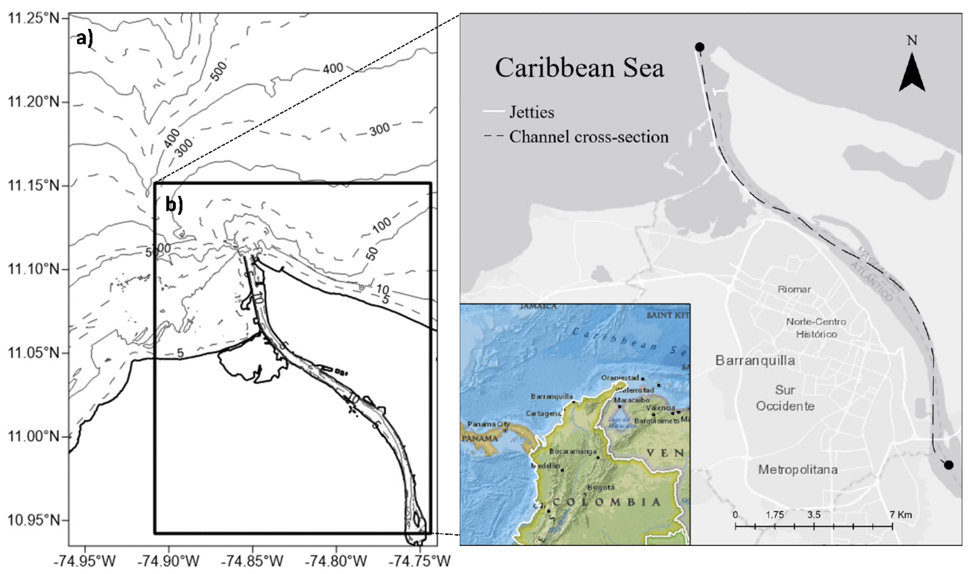
Figure 2.
Tidal periods employed for spring and neap modeling scenarios.
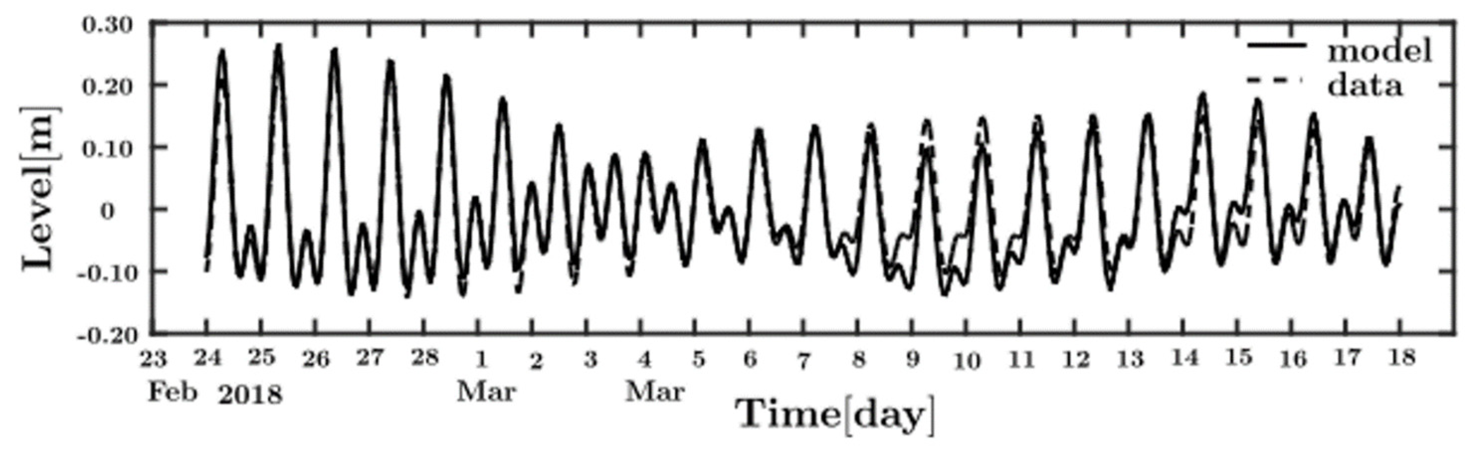
Figure 3.
Average flow regime at the estuary of the Magdalena River: (A) During wet season; (B) During dry season.
Figure 3.
Average flow regime at the estuary of the Magdalena River: (A) During wet season; (B) During dry season.
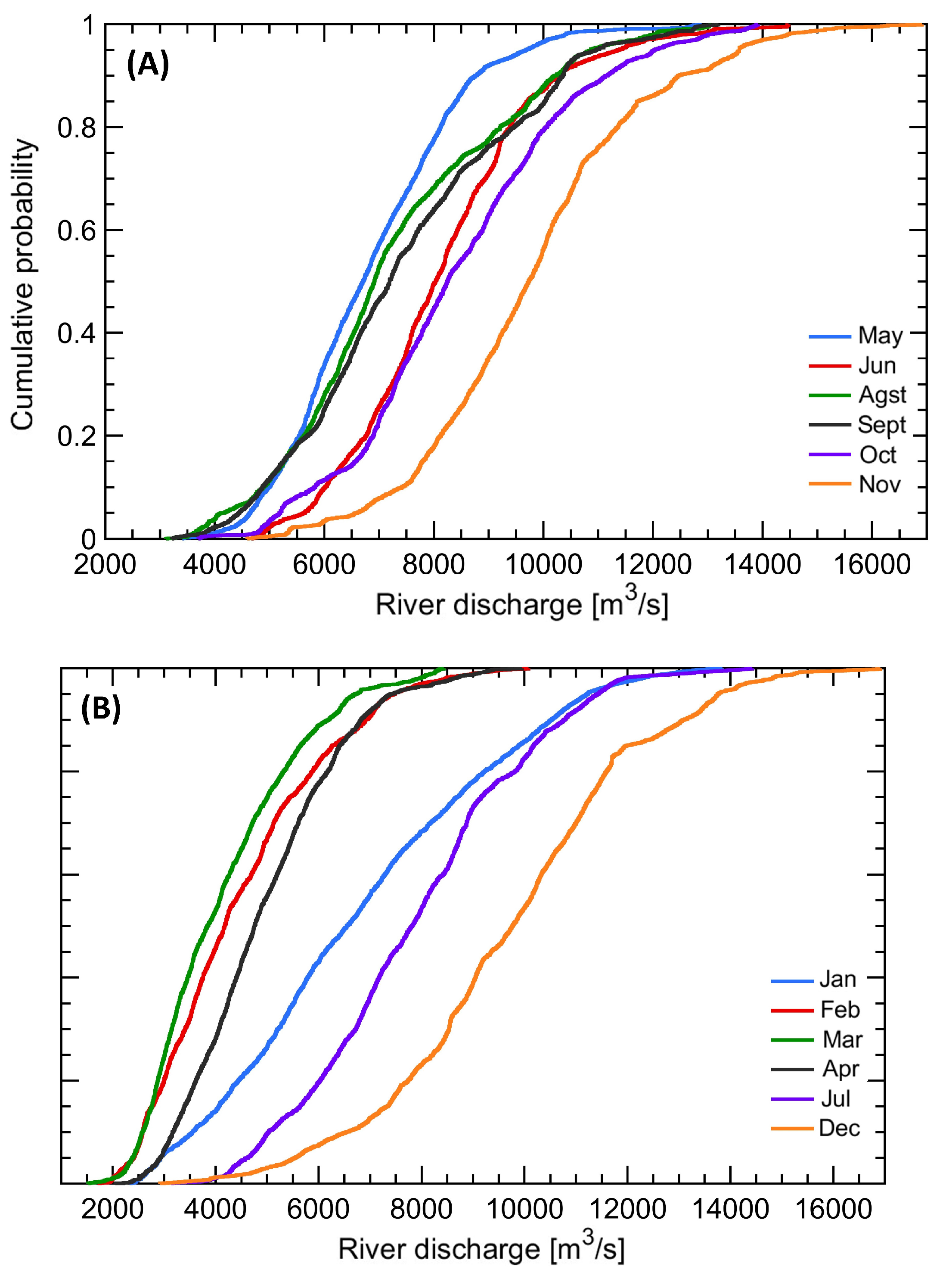
Figure 4.
Physical parameters during quadrature tides: (A) stratification; (B) buoyancy frequency; (C) potential energy anomaly; (D) bottom turbulent energy production.
Figure 4.
Physical parameters during quadrature tides: (A) stratification; (B) buoyancy frequency; (C) potential energy anomaly; (D) bottom turbulent energy production.
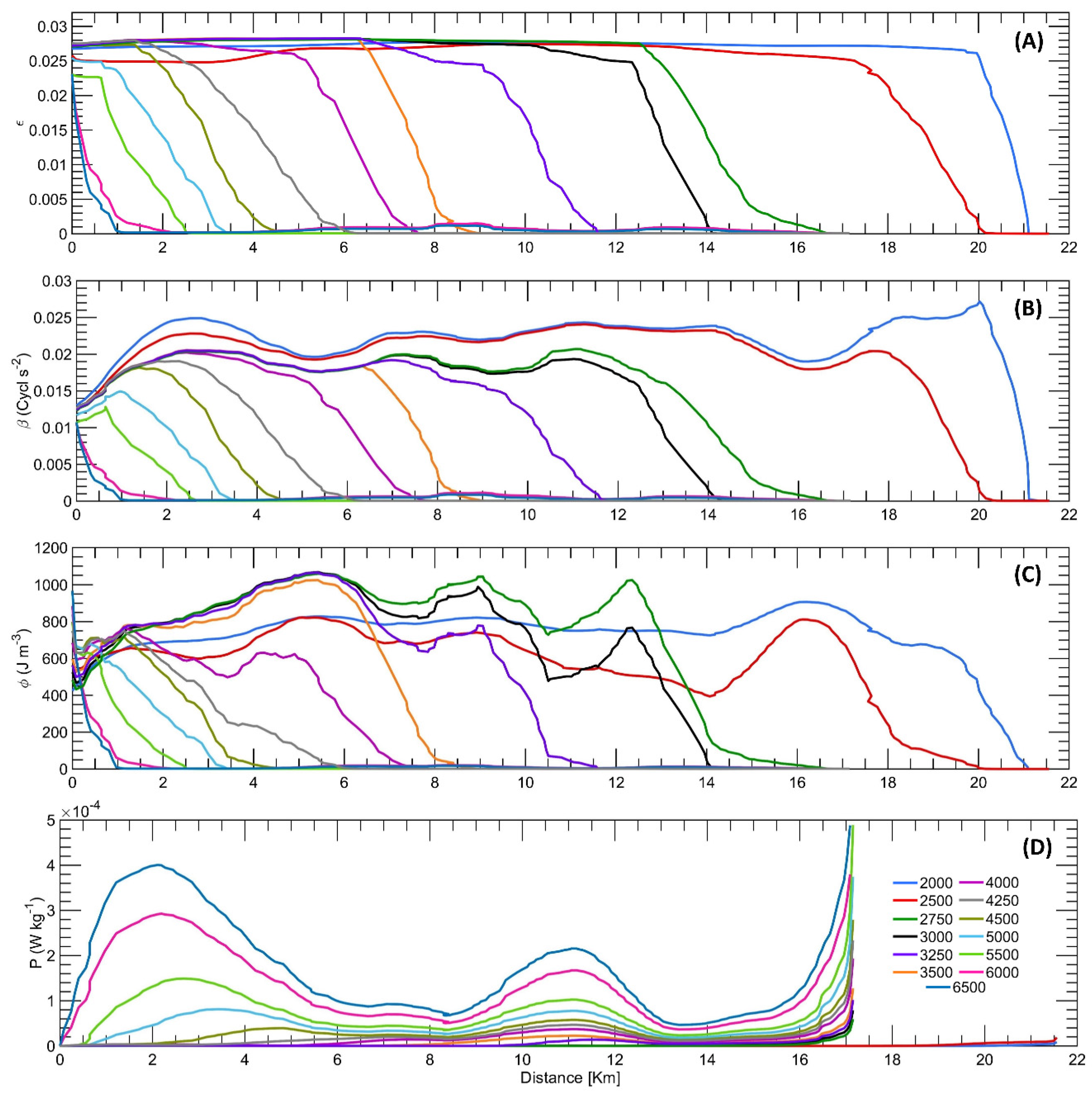
Figure 5.
Physical parameters during syzygy tides: (A) stratification; (B) buoyancy frequency; (C) potential energy anomaly; (D) bottom turbulent energy production.
Figure 5.
Physical parameters during syzygy tides: (A) stratification; (B) buoyancy frequency; (C) potential energy anomaly; (D) bottom turbulent energy production.
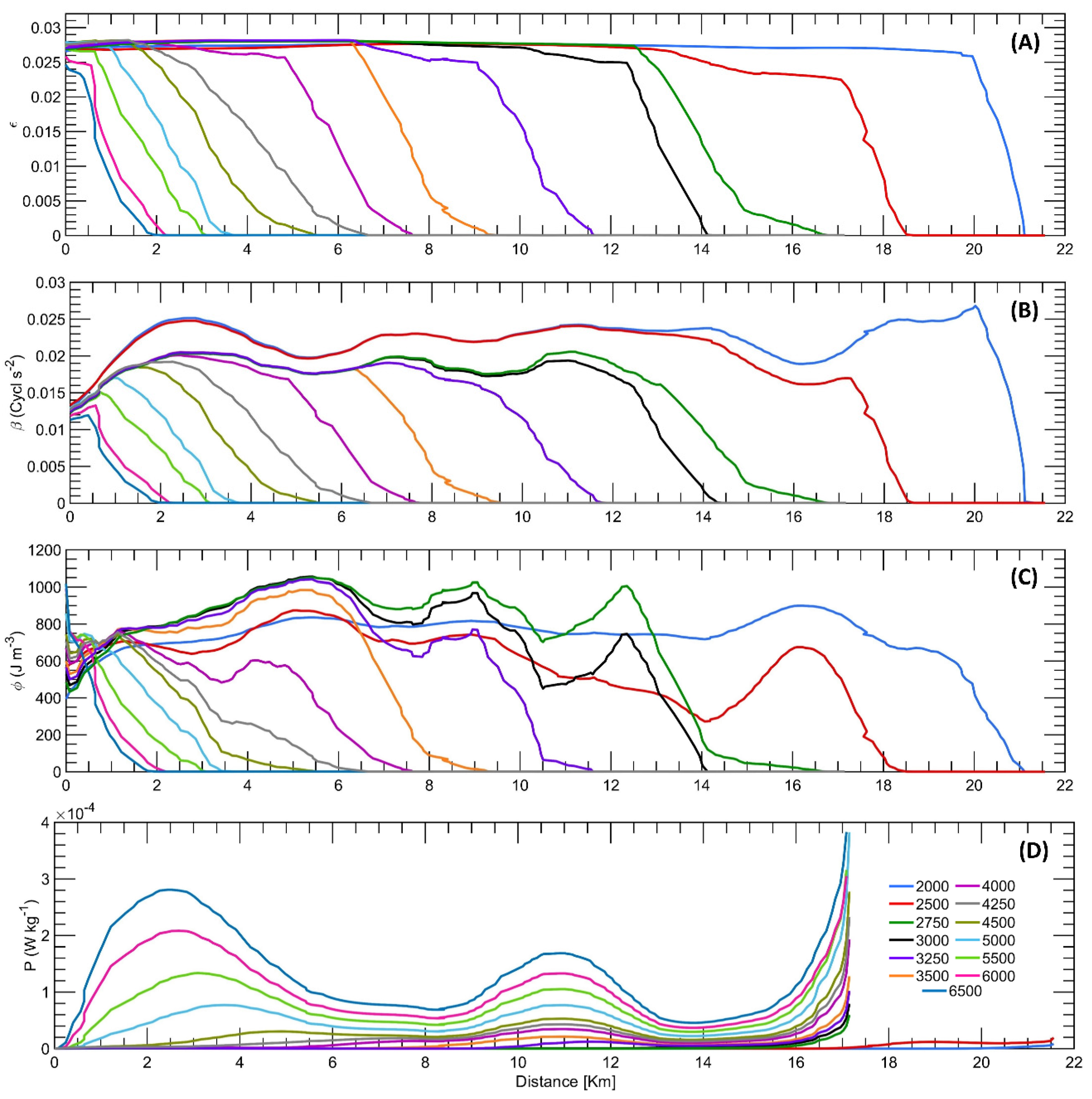
Figure 6.
Richardson by layers (RL) at Quadrature Tide in: (A) all flow scenarios; (B) depicts only the flow rates of 2000 and 2500 m3/s. (C) the flow rates ranging from 3000 to 6500 m3/s.
Figure 6.
Richardson by layers (RL) at Quadrature Tide in: (A) all flow scenarios; (B) depicts only the flow rates of 2000 and 2500 m3/s. (C) the flow rates ranging from 3000 to 6500 m3/s.
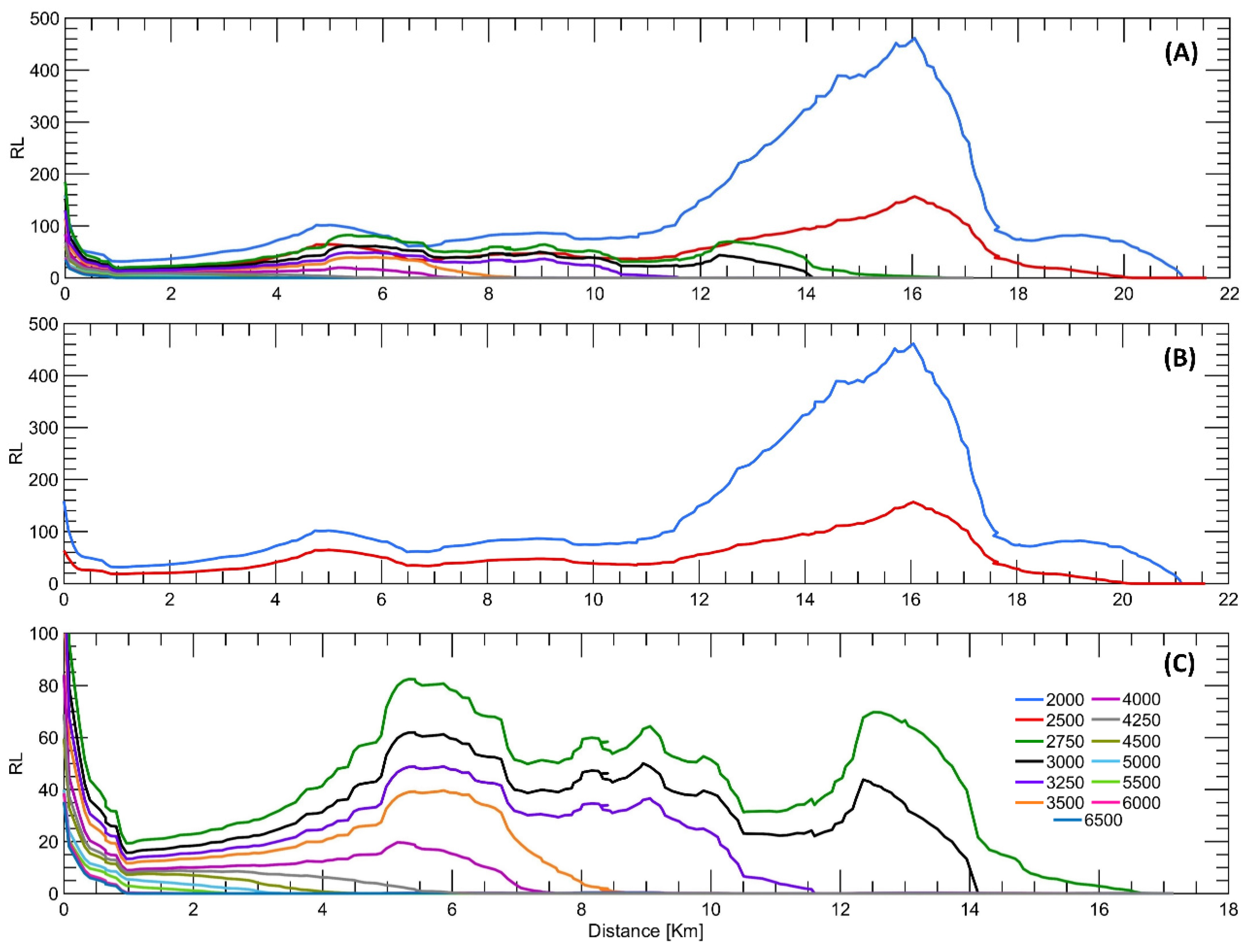
Figure 7.
Richardson by layers (RL) during Syzygy Tide in: (A) all flow scenarios; (B) depicts only the flow rates of 2000 and 2500 m3/s. (C) the flow rates ranging from 3000 to 6500 m3/s.
Figure 7.
Richardson by layers (RL) during Syzygy Tide in: (A) all flow scenarios; (B) depicts only the flow rates of 2000 and 2500 m3/s. (C) the flow rates ranging from 3000 to 6500 m3/s.
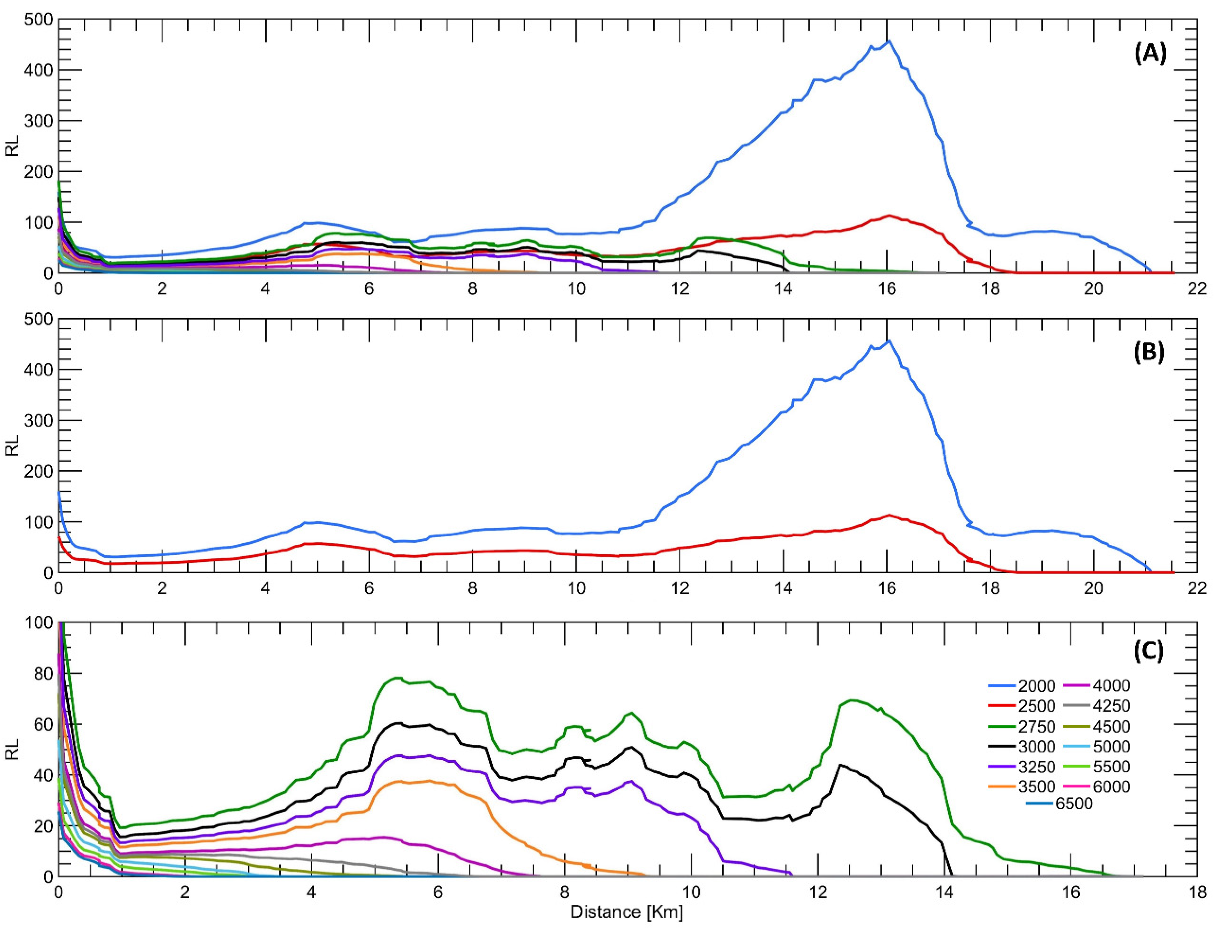
Figure 8.
Position of FSI in relation to the flow of the Magdalena River. Fitting Formula. FSI (Q) = 1.133 x 10⁻⁶ Q2 – 0.0142 Q + 46.2825 with a R2 = 0.9846.
Figure 8.
Position of FSI in relation to the flow of the Magdalena River. Fitting Formula. FSI (Q) = 1.133 x 10⁻⁶ Q2 – 0.0142 Q + 46.2825 with a R2 = 0.9846.
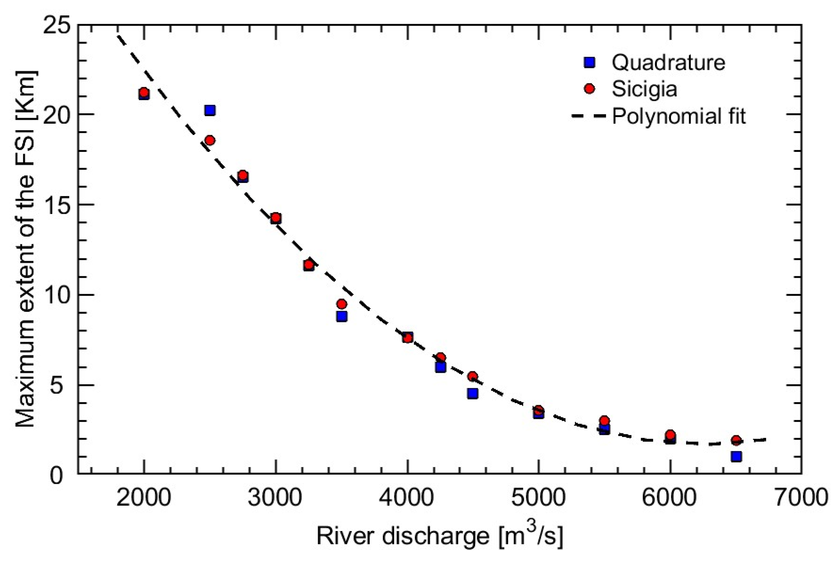
Figure 9.
Monthly ECDF of flows for the year 2016.
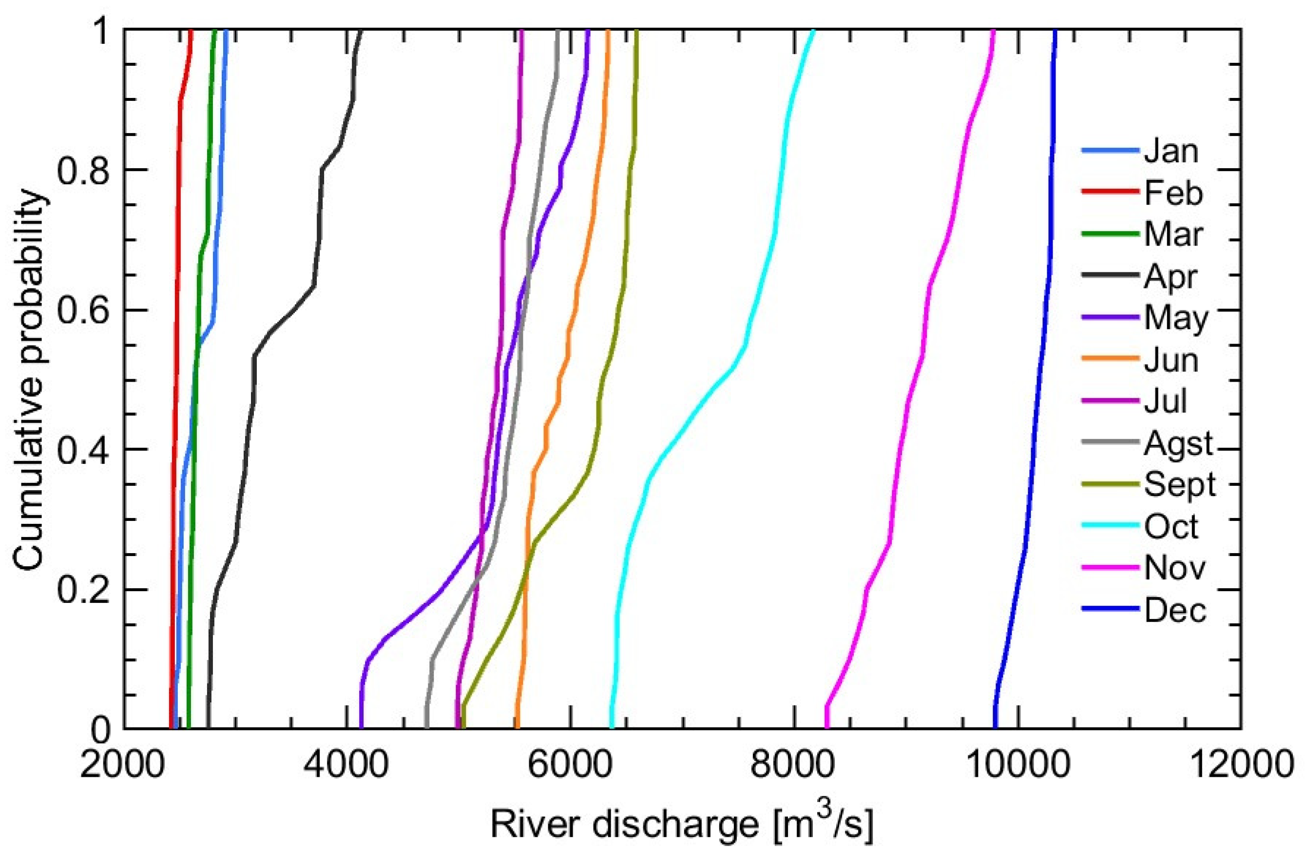

Table 1.
The Bias, RMSE and Willmott scores of the implemented MOHID model.
| Feature | Bias | RMSE | Willmott | Source |
|---|---|---|---|---|
| Salinity | 0.04 gr/kg | 0.52 gr/kg | 0.95 | |
| Velocity | 0.0085 m/s | 0.0034 m/s | 0.7568 | Higgins et al., 2022. |
| Water level | < 0.01 m | < 0.01 m | 0.91 - 0.96 | |
| Potential energy anomaly | - 0.05 | 6.2 | 0.99 | |
| Buoyancy frequency | - 0.0477 | 0.00014 | 0.99 | Otero et al., 2021. |
| Richardson number | - 0.08 | 0.13 | 0.99 |
Table 2.
Stratification and Mixing Parameters.
| Parameter formulation | Meaning |
|---|---|
| Stratification ( |
It is a dimensionless measurement of the stratification intensity based on the density of the water column. Here, the density gradient is represented by ∂ρ=ρ(bottom)- ρ(surface) and the average density is expressed as ρo=0.5 (ρb+ ρs). Usually, this parameter reaches values between 0 (indicating a well-mixed water plot) and 0.025 (indicating a highly stratified water plot) [8]. |
| Buoyancy Frequency ( |
It is a cycle/s2 index of the oscillation frequency of a vertically displaced water plot (β>0) while tending to balance hydrostatically. Here, g represents the gravity acceleration, ∂z=z(bottom)-z(surface) is the depth gradient, and ∂ρ = ρ(bottom)- ρ(surface) represents the density gradient. As β decreases, the consumption of kinetic energy involved in the production of turbulent mixing increases, resulting in a lower degree of stratification [62]. |
| Potential Energy Anomaly |
It evaluates the work per volume unit necessary to mix a water column. Here, is defined as . h, is the water column depth, and z is the depth range. When a water column is fully salty or fresh, φ tends to zero. Its unit are J/m [63]. |
| Richardson Layered Number |
It provides an estimate of the vertical mixture intensity by comparing the buoyant force and the shear stress. When RL < 2 the turbulence generated by friction is the main mixing mechanism. For 2 < RL < 20 the mixture becomes less effective. RL > 20 indicates that the water plot is stable and homogeneous. It is dimensionless [64]. |
| Turbulence Production* |
This parameter assesses the production of bottom swirls because of the Reynolds stresses and the mean shear. Here, k is the Von Karman constant (0.41), z is the depth, is an alternative to expressing friction in terms of speed, and is the drag coefficient. It is measured in W/Kg [65]. |
* This is a Turbulence Production simplification for the bottom.
Table 3.
Mean monthly streamflow (Q), maximum streamflow (Qmax), minimum streamflow (Qmin) and discharge variability (Qmax / Qmin) of the Magdalena River per month. Data interval: 23-07-1940 to 31-12-2015.
Table 3.
Mean monthly streamflow (Q), maximum streamflow (Qmax), minimum streamflow (Qmin) and discharge variability (Qmax / Qmin) of the Magdalena River per month. Data interval: 23-07-1940 to 31-12-2015.
| Month | Q (m3/s) | Qmin (m3/s) | Qmax (m3/s) | Qmax/Qmin(m3/s) |
|---|---|---|---|---|
| January | 6822 | 2326 | 13844 | 5.95 |
| February | 4474 | 1705 | 10074 | 5.91 |
| March | 4129 | 1520 | 8434 | 5.55 |
| April | 4938 | 2053 | 9951 | 4.85 |
| May | 6854 | 3402 | 12892 | 3.79 |
| June | 8153 | 4667 | 14475 | 3.10 |
| July | 7874 | 3132 | 14425 | 4.61 |
| August | 7284 | 3109 | 13063 | 4.20 |
| September | 7464 | 3214 | 13196 | 4.11 |
| October | 8443 | 3699 | 13920 | 3.76 |
| November | 9806 | 4594 | 16913 | 3.68 |
| December | 9724 | 2916 | 16913 | 5.80 |
Table 4.
Monthly cumulative probabilities for flows between 2000 y 6500 m3/s.
| Flow Rate (m3⁄s) | Months with the highest probability of occurrence | P. Accumulated (%) |
|---|---|---|
| 2000 ≤ Q ≤ 2500 | February and March | 7.2 and 7.7 |
| 2500 < Q ≤ 3000 | February and March | 12.9 and 16.7 |
| 3000 < Q ≤ 3500 | February, March, and April | 12.0, 16.7 and 10.7 |
| 3500 < Q ≤ 4000 | February, March, and April | 13.7, 11.9 and 11.0 |
| 4000 < Q ≤ 4500 | February, March, and April | 11.0, 11.7 and 14.3 |
| 4500 < Q ≤ 5000 | February, March, April, May and September | 10.1, 10.1, 13.4, 6.6 and 6.3 |
| 5000 < Q ≤ 5500 | February, March, April, May, August and September | 8.4, 7.8, 11.5, 9.5 and 6.5 |
| 5500 < Q ≤ 6000 | January, April, May, August and September | 8.2, 10.4, 14.4, 10.1 and 6.9 |
| 6000 < Q ≤ 6500 | January, April, May, June, July, August and September | 7.0, 8.2, 11.9, 7.3, 7.6, 11.2 and10.7 |
| Q > 6500 | January, May, June, July, August, September, October, November and December | 50.5, 54.3, 82.9, 72.6, 60.7, 64.1, 85.7, 95.5 and 90.1 |
Table 5.
Monthly FSI position during Neap Tides (NT) and Spring Tides (ST).
| Month | Flow rate (m3/s) | P. Accumulated (%) | NT-FSI | ST-FSI |
|---|---|---|---|---|
| December | 6000 - 14583 | 90.1 | Km < 2 | Km < 2.2 |
| January | 3000 - 11428 | 90.0 | Km < 14.2 | Km < 14.2 |
| February | 2500 - 8350 | 90.2 | Km < 20.2 | Km < 18.5 |
| March | 2000 - 6500 | 92.2 | Km 1 y 21.1 | Km 1.9 and 21.2 |
| April | 2500 - 6976 | 90.6 | Km < 20.2 | Km < 18.5 |
| May | 3500 - 8823 | 90.1 | Km < 8.8 | Km < 9.4 |
| June | 5000 - 10909 | 91.0 | Km < 3.4 | Km < 3.6 |
| July | 3250 - 10909 | 91.0 | Km < 11.6 | Km < 11.6 |
| August | 3250 - 10243 | 90.0 | Km < 11.6 | Km < 11.6 |
| September | 3500 - 10380 | 90.0 | Km < 8.8 | Km <9.4 |
| October | 5000 - 11875 | 90.3 | Km < 3.4 | Km < 3.6 |
| November | 5500 - 13215 | 90.3 | Km < 2.5 | Km < 3 |
Table 6.
Monthly FSI position during Neap Tides (NT) and Spring Tides (ST) in 2016.
| Month | Flow rate (m3/s) | P. Accumulated (%) | NT-FSI | ST-FSI |
|---|---|---|---|---|
| December | 9800 - 10334 | 93.7 | Km ~ 0 | Km ~ 0 |
| January | 2495 - 2917 | 88.9 | Km 20.2 y 14.2 | Km 18.5 and 14.2 |
| February | 2428 - 2507 | 89.6 | Km ~ 20.2 | Km ~ 18.5 |
| March | 2583 - 2780 | 90.3 | Km 20.2 y 16.5 | Km 18.5 and 16.6 |
| April | 2760 - 4054 | 90 | Km 16.5 y 7.6 | Km 16.6 and 7.6 |
| May | 4186 - 6155 | 90.3 | Km 6 y 2 | Km 6.5 and 2.2 |
| June | 5525 - 6306 | 90 | Km 2.5 y 1 | Km 3 and 1.9 |
| July | 4988 - 5548 | 90.3 | Km 3.4 y 2.5 | Km 3.6 and 3 |
| August | 4763 - 5884 | 90 | Km 4.5 y 2 | Km 5.5 and 2.2 |
| September | 5041 - 6573 | 90 | Km 3.4 y 1 | Km 3.6 and 1.9 |
| October | 6412 - 8177 | 90.3 | Km < 1 | Km < 1.9 |
| November | 8294 - 9650 | 90.0 | Km ~ 0 | Km ~ 0 |
Disclaimer/Publisher’s Note: The statements, opinions and data contained in all publications are solely those of the individual author(s) and contributor(s) and not of MDPI and/or the editor(s). MDPI and/or the editor(s) disclaim responsibility for any injury to people or property resulting from any ideas, methods, instructions or products referred to in the content. |
© 2023 by the authors. Licensee MDPI, Basel, Switzerland. This article is an open access article distributed under the terms and conditions of the Creative Commons Attribution (CC BY) license (http://creativecommons.org/licenses/by/4.0/).
Copyright: This open access article is published under a Creative Commons CC BY 4.0 license, which permit the free download, distribution, and reuse, provided that the author and preprint are cited in any reuse.


