
Submitted:
11 November 2023
Posted:
13 November 2023
You are already at the latest version
Abstract
Recently, significant progress has been made in developing computer-aided diagnosis (CAD) systems for identifying glaucoma abnormalities using fundus images. Despite their drawbacks, methods for extracting features such as wavelets and their variations, along with classifier like support vector machines (SVM), are frequently employed in such systems. This paper introduces a practical and enhanced system for detecting glaucoma in fundus images. This system adresses the chanallages encountered by other existing models in recent litrature. Initially, we have employed contrast limited adaputive histogram equalization (CLAHE) to enhanced the visualization of input fundus inmages. Then, the discrete ripplet-II transform (DR2T) employing a degree of 2 for feature extraction. Subsequently, a golden jackal optimization algorithm (GJO) employed to select the optimal features to reduce the dimension of the extracted feature vector. During the classification stage the least square support vector machine (LS-SVM) with three kernels called as linear, polynomial and radial basis function(RBF), for classifying of fundus images as glaucoma or healthy. The proposed method is validated with the current state-of-the-art models on two standard datasets, namely, G1020 and ORIGA. The results obtained from our experimental result demonstrate that our best suggested approach DR2T+GJO+LS-SVM-RBF obtains better classification accuracy 93.38% and 97.31% for G1020 and ORIGA dataset with less number of features. It establishes a more concise network structure when contrasted with traditional classifiers.
Keywords:
IOP
; ONH
; CLAHE
; GJO
; DR2T
; LS-SVM
1. Introduction
Glaucoma is a condition that affects the optic nerve and results in an anomaly in the eye’s drainage system. This can lead to fluid buildup, resulting in increased pressure that has the potential to damage the optic nerve. This leads to a distinct optic nerve head appearance during fundoscopic evaluation and a corresponding gradual decline in vision. For the preservation of life, early screening detection is crucial to prevent the loss of vision. Approximately four million individuals in the United States are believed to suffer from glaucoma, with half unaware of their condition. Out of these, around 120,000 have experienced blindness due to glaucoma, constituting about 9% to 12% of all cases of blindness in the country. Elevated intraocular pressure (IOP) affects approximately 2% of those aged between 40 and 50 and about 8% of individuals aged over 70 [1]. Hence, it is imperative to include glaucoma screening as an integral aspect of continuous healthcare. The primary methods for detecting glaucoma encompass evaluating intraocular pressure (IOP) [2], conducting visual field tests [3], and analyzing the configuration of the optic nerve head (ONH) [4]. Numerous research endeavours have been undertaken to create computer-aided diagnosis (CAD) systems to identify glaucoma early. Certain illnesses result in minor issues with the human eye, while others can result in permanent loss of vision. Hence, Developing a computer-aided diagnostic (CAD) system specialized for glaucoma detection in human eyes through fundus images, which automates the work of an ophthalmologist, is of utmost importance. It plays a crucial part in making accurate and timely clinical judgments. Fundus imaging, an advanced method in medical imaging, is commonly used to acquire images of the glaucoma-affected fundus due to its capacity to efficiently transform data associated with eye conditions in the human eye. Hence, if there is damage in the optic nerve, the communication between the eye and brain becomes stopped. In addition, Glaucoma is a non-invasive imaging technique that doesn’t require invasive procedures or expose the patient to radiation, unlike other options like CT scans and X-rays. Manually analyzing fundus images to make this detection is time-consuming; expensive, inconvenient process which is complicated scheme that requires expert supervision. To tackle these difficulties, it’s crucial to develop an automated computer-aided design (CAD) model using a dedicated computing system. This system can assist ophthalmologists in making faster and more accurate judgments by integrating various image processing and pattern recognition algorithms at various points in the process. Researchers have noted that the discrete wavelet transform (DWT) is primarily utilized as a feature extraction tool in the realm of image processing. This application involves the identification of features in fundus images across various scales while also addressing singularities in one-dimensional (1D) data. Hence, Defining two-dimensional (2D) singularities, like the boundaries of fundus images, has proven to be a challenging task with limited precision. So, DWT struggles to effectively capture curve-like characteristics in fundus images. Hence, there is a significant need for enhanced changes to tackle these concerns. Therefore, the classifier, specifically the support vector machine (SVM), has been utilized for the classification of CAD models due to its ability to discriminate between nonlinear input patterns and make predictions for continuous functions. Hence, The traditional SVM classifier encounters greater computational complexity and exhibits subpar performance when handling large datasets. Moreover, certain fundus image necessitate more features, thereby complicating and increasing the burden on the classification task. This approach utilizes specific points of interest within a multi-dimensional feature space derived from fundus images, demonstrating robustness to changes in the area near the optic disc. Machine learning (ML) has been used to tackle various tasks involving the analysis of medical images, demonstrating impressive speed and efficiency in optimizing processes across a wide range of diseases, such as breast cancer diagnosis [5,6,7,8,9,10], diabetes detection [11,12], etc.
In this paper, we have developed an efficient CAD model that can tackle the difficulties faced by existing models. The deployed scheme has significantly improved by introducing the ripplet-II transform and a novel version of the least-square support vector machine (LS-SVM) with different kernels in the suggested system. The research study contributes explicitly in the following ways:
- Utilizing the discrete ripplet-II transform (DR2T) for feature extraction offers benefits by effectively capturing two-dimensional irregularities and a group of curves in fundus images.
- The golden jackal optimization (GJO) aimed to select the most essential elements from the range of potential solutions, with the goal of eliminating redundant and irrivalant features and LS-SVM (GJO+LS-SVM) to classify better classification accuracy.
- The LS-SVM acts as the classifier and provides a higher level of computational efficiency compared to the conventional SVM.
- Comparison with alternative capable techniques based on classification accuracy and quantity of attributes using three widely recognized datasets.
- The remainder of this article is organised as follows: In Section 2 provides a summary of the literature regarding glaucoma detection. Section 3 provides a comprehensive explanation of our approach, encompassing the suggested methodology. Section 4 explored the experimental discoveries and evaluated the outcomes. This Section 5 highlights the summarization of the research’s results and delineates possible directions for future research.
2. Related works
In contemporary methods for detecting glaucoma through categorization reliant on distinguishing features, either the entire fundus image or a portion of the retina that includes the optic disc is employed for feature extraction. To extract and consolidate the methods and characteristics of significant advancements in utilizing machine learning (ML) for the classification and diagnosis of glaucoma. Yin et al. [13] presented a new computer aided diognisis (CAD) model that exprimented on four ocular conditions linked to an online platform through a cloud-based system and SVM used as a classifer for glaucoma detection. In [14] the authors used a new CAD model based on contrast-limited adaptive histogram equalization (CLAHE) techniques to extract features from unlabel datasets, that leads to avoiding overfitting problem. Maheswari et al. [15] have implemented a novel approach for detecting glaucoma by utilizing empirical wavelet transform (EWT) to break down the images and extract correntropy features and used the least-squares support vector machine (LS-SVM) as classification of glaucoma. In [16], the authors have deployed a new CAD model by utilizing the Variational Mode Decomposition (VDM) technique for image decomposition, various features such as Kapoor entropy, Renyi entropy, Yager entropy, feature dimension for VDM component extraction, and employing LS-SVM for classification were applied. Kausu et al. [17] have employed features derived from the dual-tree complex wavelet transform, used fuzzy c-means clustering methods and Otsu’s optic-cup segmentation thresholding. In [18], the authors have presented optic disc localization, the non-parametric GIST descriptor, that is used to reduce using locality sensitivity discriminant analysis (LSDA) through different feature selection and ranking schemes and classification. Parashar et al. [19] utilized a novel CAD approch to diagnosis of glaucoma, employing wavelet analysis to break down fundus images into multiple modes. Subsequently, we extract fractal dimension (FD) and diverse entropy measures to capture and construct a least square support vector machine (LS-SVM) model with various kernel functions. In [20], the authors have used a new CAD model employing machine learning methodologies, a deep sparse autoencoder was introduced. This model was designed to amalgamate attributes from deep and primary features, improving the overall effectiveness of representing advanced features and potentially enhancing the efficiency of expressing high-level features. Furthermore, the model integrates L1 regularization to augment the synergy of deep features, especially in situations with a scarcity of sample data.Recent literature emphasizes the prominent role of machine learning, especially within ensemble learning methods. This is particularly beneficial in the biomedical domain, even when datasets are scarce. Presently, many models rely on machine learning approaches, yet no prior research has concentrated on ensemble methods for classifying glaucoma. Therefore, our proposed study centers on ensemble learning, leveraging the combined power of XGBoost, support vector machines (SVM), and logistic regression (LR) to achieve superior classification outcomes compared to conventional models. In [21], the aurhors employed DWT and HOG characteristics are followed by an ELM classifier. Additionally, in [22],the authors deployed a novel CAD model is described, where correlation attributes are chosen through a bio-inspired algorithm, and a KELM classifier based on salp-swarm optimization is applied. Latif et al. [23] have introduced a model that utilizes Speeded-Up Robust Feature (SURF) and histogram of oriented gradients (HOG) features. In this model, we’ve incorporated an improved version of the grey wolf optimization (GWO) technique alongside a SVM for classification. Raja et al.[24] have obtained extracted statistical features using hyper-analytic wavelet transformation (HWT). Furthermore, They applied a hybrid particle swarm optimization (PSO) algorithm with a diverse particle population and employed a support vector machine (SVM) for classification of glaucoma diagnosis.[12].
In the literature, most of the computer-aided diagnosis (CAD) models cannot provide a good classification result. Schemes in the literature have higher computational complexity and are unsuitable for real-time applications. Many existing CAD models rely on handcrafted feature extraction procedures. Almost all CAD approaches are focused on different machine-learning algorithms. Choosing the right features and effectively categorizing them have remained a crucial challenge.
3. Proposed methodology
The employed scheme is based on four prime sections: preprocessing of fundus images, feature extraction, feature selection and classification. Figure 1. shows the architecture using the employed scheme’s computer-aided diagnosis (CAD) model. Each section has described in detail.
3.1. Preprocessing
In our proposed research, we have divided the glaucoma datasets into a 60:40 ratio for training and testing to achieve the highest level of accuracy. This research focuses on two well-known datasets: G1020 [25] and ORIGA images [26]. To improve the quality of our dataset, we applied a cropping process to extract relevant regions of interest (ROI). Ophthalmologists provided the cup and disc values on numerous images. Our approach primarily centred on cropped images resized at 256 × 256 pixels. In cases where specific ROIs were unavailable due to a lack of prior knowledge, the entire 256 × 256 image has been considered. We have specified sample images from both datasets illustrated in Figure 2, and some sample image details are tabulated in Table 1.
3.1.1. Prepocessing based on CLAHE method
To establish a balance within the shared input space, we have employed contrast limited adaptive histogram equalization (CLAHE) technique, commonly used in image processing [27]. Unlike adaptive histogram equalization (AHE), CLAHE offers advantages such as avoiding excessive noise amplification and reducing the occurrence of edge-shadowing effects [28]. This method enhances image contrast by redistributing intensity values, making image details more distinguishable. Traditional histogram equalization can have drawbacks, such as amplifying noise and not considering local image characteristics. CLAHE addresses these issues by applying adaptive histogram equalization locally, ensuring that contrast enhancement is limited to a specified level.
3.2. Feature extracton using discrete ripple-II transform (DR2T)
In image processing, feature extraction involves distilling vital data from images to simplify their complexity, making them suitable for tasks like recognizing objects and analyzing patterns. This is achieved through edge detection and texture analysis, which help identify and depict significant image attributes.
The fourier transform is less effective for extracting features from images due to its inability to retain temporal information and manage 1D singularities. Consequently, it fails to depict images containing edges effectively; nevertheless, it performs admirably when applied to images with smoother features. On the other hand, the wavelet transform excels in depicting one-dimensional singularities, also referred to as point singularities. However, the traditional wavelet transform cannot effectively capture two-dimensional singularities occurring along curves of arbitrary shapes. To address the issue inherent in traditional wavelets, an alternative transformation known as the ridgelet transform was introduced. This transformation relies on the Radon transform and aims to provide a solution to the aforementioned problem [29,30]. Ridgelet shows significant promise in capturing linear singularities (meaning it can identify lines with various orientations), yet it must work on effectively dealing with two-dimensional singularities. Subsequently, Candes and Donoho introduced the initial iteration of the curvelet transform using a multiscale ridgelet approach, aiming to address singularities occurring along smooth curves in 2D. Subsequently, they unveiled an enhanced iteration of the curvelet transform, labeled as the fast discrete curvelet transform (FDCT). Such recent iteration is characterized by its simplicity, speed, and reduced redundancy compared to its predecessor [31]. Due to features such as multi-resolution, increased directional sensitivity, anisotropy, localization, and more, it has captured significant interest in recent decades. The characteristic of anisotropy ensures the resolution of 2D irregularities along smooth C2 curves. To achieve this, curvelet employs a scaling principle that resembles a parabolic pattern [32]. Nevertheless, the rationale for choosing parabolic scaling remains to be determined. A novel transformation known as the ripplet-I transform is introduced to address this concern. This transformation offers a broader application of the scaling principle [33,34]. The ripplet-I transform expands upon the idea of the curvelet transform by introducing two extra parameters: the support parameter denoted as c and the degree parameter denoted as d. Here, , the ripplet-I transform as the curvelet transform. These two factors equip the ripplet-I transform based on ability to portray anisotropy, allowing it to depict 2D singularities along curves of various shapes. Next, they introduced the ripplet-II transform [35], which builds upon the generalized Radon transform (GRT)[36,37], aiming to enhance the effectiveness of capturing 2D singularities. It fulfils multi-resolution, localisation, and strong directionality and flexibility. In contrast to the wavelet and ridgelet transforms the ripplet-II transformation exhibits the swiftest coefficient reduction. This enables a more concise representation of images containing edges. Moreover, it possesses the characteristic of being invariant to rotation. It can provide rotation-independent characteristics, sparse feature vectors, that are essential for glaucoma detection purposes. Consequently, it has been utilized in texture detection and image feature extraction tasks [35]. Because of its exceptional ability to capture edges and textures, which surpasses that of conventional transforms, the ripplet-II transform is employed as the feature extraction method in this research. This choice is driven by the presence of edges and textures with diverse shapes within the impacted areas of fundus images.
3.2.1. Ripplet-II transform
Here, a 2D function g(x,y), the continious ripplet-II transform in polar coordinates can be specified as’
where, g shows as the polar coordinate conversion of g(x,y), is named as ripplet-II function and is the complex conjugte of . The ripplet-II function defined as
Here, has a smooth univariate wavelet method and shows scale, translation, degree, and orientation parameters, accordingly. The ripplet-II transform can capture structural information along arbitrary curves by tuning these hyperparameters. using Equation 1 and 2, we have
Hence, has the GDT function g and shown as:
Hence, the GRT can be calculated using Fourier transform [35]. Equation 3 viewed as ripplet-II transform is the inner product of GRT and 1D wavelet, which shows in :
Here, we have defined that ripplet-II transform works in two steps: firstly compute GRT of g and then evaluate 1D WT of the GRT of g. The discrete version of ripplet-II transform (DR2T) can be specified as
Where the discrete GRT(DGRT) of g is first evaluated, the 1D discrete WT (DWT) of the DGRT of g is evaluated. The computing method for the discrete ripplet-II transforms, which is more straightforward when d=2. In this case, the GRT is dubbed ’parabolic Random transform’ and specified as[35].
Here, having the classical random transform (CRT) in polar coordinates. Hence, the GRT of function g for d>0 takes the form of Fourier domain as:
Here, shows the Chebyshev polynomial of degree n. Finally, the forward DR2T having d=2 of an input image can be evaluated as:
- Convert the input function from Cartesian coordinates to polar coordinates, which is to . Update by in . Hence, construct a new image by interpolation after converting polar coordinates to Cartesian cordinates(x,y). Here, the variables x and y store integer values.
- deployed discrete CRT on that generates and then substitue with in as in Equation 7. then obtain the DGRT coofficients .
- Consider 1D-DWT to DGRT coefficients w.r.t and obtain the discrete ripplet-II coefficients.
The above substitution from to creates DR2T coefficents more sparser than others.
3.2.2. Feature generation using DR2T
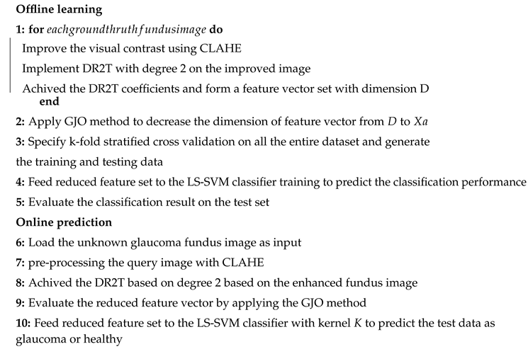
In our deployed work, DR2T has been utilized as the feature extractor. We applied DR2T and obtained the coefficients for every training input glaucoma image. Then, the transform coefficients are organised in a feature vector of dimension D, where D = m * n, and m and n are the number of rows and columns of the image. This vector is derived for every training fundus image, and a feature matrix is formed. Hence, the implementation method of the feature generation is outlined in the Algorithm 1.
| Algorithm 1:Feature extraction based on discrete ripplet-II tansform |
|
3.3. Feature Selection using meta-heuristic optimization techniques
Metaheuristic optimization methods are adaptable algorithms employed for tackling a diverse array of intricate optimization challenges. They provide advantages such as the ability to handle various problems independently, conduct global searches, offer flexibility, ensure computational efficiency, and maintain resilience. There are number of meta-heuristic techniques like, gnetic algorithms (GA) [9], simulated annealing (SA) [10], particle swarm optimization (PSO) [11] and ant colony optimization (ACO) [12] etc. In our suggested model, we have used golden jackal optimization (GJO) [13] for feature selection is crucially significant within the context of picking out the most significant image characteristics to decrease complexity and enhance the effectiveness of tasks. The GJO algorithm excels in its capacity to efficiently address intricate optimization problems by harnessing the insights derived from the behavior of jackals. Typical approaches involve using statistical measures and machine learning algorithms to preserve essential data while eliminating redundant information.
3.3.1. Golden Jackal Optimization Algorithm
The Golden Jackal Optimization (GJO) technique draws its inspiration from the hunting and feeding habits of golden jackals, serving as a meta-heuristic optimization approach. This approach seeks to replicate the versatile predators’ adaptive hunting tactics, renowned for their capacity to flourish in a wide range of environments. GJO endeavours to tackle optimization problems with efficiency and effectiveness [13]. It’s following are the key steps in the search for a pair of golden jackals:
- Finding the target and moving closer to it.
- Catching the quarry and provoking it.
- Hunting down and capturing the prey.
Like many other meta-heuristic approaches, the GJO utilizes a strategy centered around a population, commencing with an initial solution randomly distributed throughout the entire exploration region, as demonstrated in Equation 9.
Here, is denoted as the lower bound, is specified as the upper bound, shows a method that ranges from 0 to 1. Hence, () specified as initial matrix Prey in Equation 10. During the initialization phase, a pair of jackals emerged as the top two most fitness members in the group that was created.
Equation 10 demonstrates, ’p’ represents the prey, while ’q’ represents the attributes. The attributes of a specific outcome are mirrored by the position of each potential target. In the course of optimization, a fitness function is employed to evaluate the appropriateness of each target as described in Equation 11, all the fitness values of the prey are gathered within a matrix, with the F matrix containing these values for each individual prey. In this context, represents the component of the prey’s dimension. The optimization problem pertains to a group of ’p’ preys, we represent the objective method as F. When studying the hunting patterns of golden jackals, the main focus is on the male jackal, while the female jackal is considered a secondary fittness. The hunting pair collaboratively determines the locations of their prey respectively.
Because of their inherent characteristics, jackals excel at detecting and chasing after prey. However, there are occasions when the prey manages to elude them, leading the jackals to explore other potential targets, a phase called as stage of exploration. While engaged in hunting, the male jackal assumes the role of the pack’s leader, taking charge of the pursuit, with the female jackal closely trailing behind. Equations 12 and 13 Show the changing the male jackal’s location in each iteration, indicated by ’i’. The female jackal’s location is denoted as XFM, while X represents the position of the male jackal, and Xprey viewed as the place of the prey. Bases on current location the male jackal is referred on , while the adjusted location based on female jackal as she pursues the prey is labeled on . The energy expended by the prey as it tries to escape is quantified as ’e’ and is established using the following method in Equation 14.
So, represents the initial energy level, while signifies the declining energy of the prey.
The variables in Equations 15 and 16 consist of ’r,’ a random integer with values ranging between 0 and 1, and ’c1,’ which remains constant based on 1.5. The ′I′ shows the maximum number of iterations, while ’i’ stands for the ongoing iteration. Additionally, ’e1’ experiences a gradual reduction from 1.5 to 0 as the iterations progress. Equations 12 and 13 deal with the calculation involves determining The gap separating the jackal from its target, viewed as . Considering the prey’s evasive energy, the jackal’s current position remains unchanged, with no addition or subtraction of distance. Two equations are utilized, with vector generating a series of random numbers following the Levy distribution, representing the Levy position. To assess the prey’s location in a Levy sequence, the equation represents the vector alongside the prey vector as visualized in Equation 17.
In Levy flight technique, specified as , has assessed based on Equation 18 and 19. In this context, ’v’ ranges from 0 to 1, and the value of is established at 1.5.
At the end, Equation 20 specified as the new jackal positions are determined by averaging the results of the Equations 12, 13.
In our computational approch, we demonstrate the collaborative hunting behaviors of a male, female jackal through the use of mathematical Equations 21, 22. In this particular scenario, ’i’ stands for the ongoing iteration, ’’ symbolizes the prey’s position vector, ’’ specified as male jackal’s location, ’’ represents based on position of female jackal. ’’ specified as the updated location based on male jackal, while ’’ signifies as updated location of the female jackal based on prey. For updation in jackals’ positions are specified by Equations 14 and 20, that are used for calculating the prey’s evasion energy. In order to prevent becoming trapped in local optima and encourage the pursuit of new possibilities, Equations 21, 22 integrate on ’’ method. In Equation 17, assessing ’’ with the aim of reducing the likelihood of becoming trapped in suboptimal situations, particularly in the latter phases, mirrors the difficulties jackals encounter while hunting in their native environment. During the exploitation phase, ’’ grapples with these challenges.
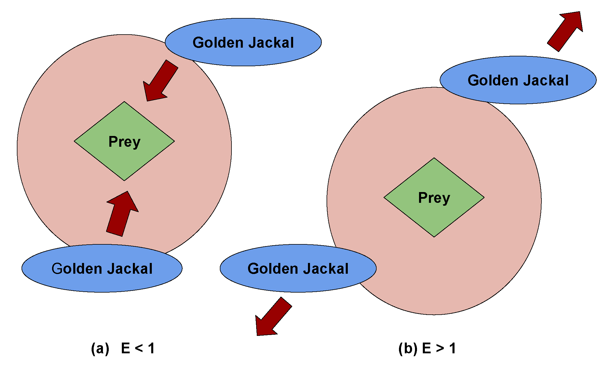
Lastly, the GJO algorithm initiates by forming a randomized collection of prey to serve as a potential solution. In every cycle, the jackals work together to predict where their prey might be located. Within the group, each jackal update the distances between pairs of jackals based on a preset rule. As time goes on, the parameter e1 decreases gradually between 1.5 to 0 to achieve equilibrium between the pursuit of new opportunities and the utilization of existing resources. When the value of e surpasses 1, the golden jackal sets distance themselves based on prey. Conversely, e drop below 1, the teams move closer to the prey in an attempt to improve their odds of capturing it.
3.3.2. Feature selection using golden jackal optimization algorithm (GJO)
Feature selection involves the deliberate choice of a more focused subset of input variables from a larger dataset. The main goal is to improve the precision of machine learning models, reduce computational demands, and reduce the chances of overfitting. This technique aims to identify the most vital features that significantly influence the target variable. Selecting the appropriate features for classification can pose a challenge, and this is where GJO optimization comes into play. GJO optimization is used to identify a relevant subset of features. By utilizing GJO, we achieve a boost in classification accuracy. The subsequent segments offer a comprehensive elucidation of the distinct phases involved in GJO.
- Initialization: GJO employs a population-centric strategy, much like several other metaheuristic techniques, wherein it uniformly explores the search space, commencing from starting phase. The starting result specified in Equation 23, In this context, represents the minimum limit, signifies the maximum limit, and ’rand()’ is a method that produces values within the range of 0 to 1.Suppose we have ’p’ possible prey items and ’q’ variables that each individual can exhibit, as outlined in the Equation 24. In this context, ’i’ ranges from 1 to ’p’, with each ’i’ representing the position of a single prey’s. Consequently, the prey groups can be represented based on ’p × q’ vector denoted by , as described, Equation 25. Here, ’i’ takes values , and , with each row representing an individual prey, and each column representing a specific variable or dimension. symbolizes the initial prey matrix established during initialization, comprising the two healthiest individuals, one male, and one female jackal.Utilizing an optimization approach involving a set of p prey entities and q variables, the position of each prey entity unveils the characteristics of a particular solution. A performance evaluation function, also referred to as a fitness function, it is used to evaluate the effectiveness of each potential solution during the optimization process. The outcomes of this function for all conceivable solutions have been recorded in a matrix, as illustrated in Equation 26. In this equation, the variable ’i’ ranges from 1 to ’p’ and ’j’ from 1 to ’q’. We capture the performance metrics for each prey in a matrix denoted as . The optimization procedure includes ’p’ prey individuals, and their performance is evaluated using the designated objective function denoted as . The male and female jackals are considered to be the most and second-most adept prey individuals, respectively, often referred to as male jackal and female jackal prey positions.
- Exploration Phase: In golden jackal optimization (GJO) method, exploration has achieved based on simulating the actions of a group of golden jackals as they forage for food in an unknown environment. Every jackal, representing a potential result, undergoes random movement based on specified limit to enhance the search area which random movement strategy prevents the algorithm from getting stuck in local optimal solutions and promotes the discovery of novel solutions. Occasionally, the prey may elude capture, but jackals are naturally adept at sensing and tracking it. Consequently, when the prey proves elusive, the jackals explore to seek out alternative destinations. Throughout the hunt, the male jackal assumes the lead position, with the female jackal following closely behind. Equations 27 and 28 outline the process of updating the male jackal’s position in this pursuit.In this scenario, ’Xprey’ signifies the vector indicating the prey’s location, "" represents the male jackal’s location, while "" signifies the female jackal’s position. The instaces ’i’ denotes the recent iteration, while ’’ represents as updated location based on male jackal ’’. ’’ specified as the position adjusted relative to the prey based on the jackal belongs to female groups ’’. For compute the prey’s evasion energy, referred to as ’Ep,’ Equation 29 is applied. Within this equation, ’Ep0’ specified as the current energy of the prey, while ’’ represents as reduction in its energy level.Here, is determined by applying Equation 30, and is computed using Equation 31. In these equations, we utilize the variable ’r,’ a randomly generated number falling within the range of 0 to 1, along with a fix value specifed as ’c1,’ set to 1.5. Furthermore, We introduce the variables ’I’ to denote throughout the iterations and ’i’ to represent the ongoing iteration count. The variable specified as decreasing energy of the prey labeled as ’.’ Its value gradually decreases based on 1.5 to 0, Indicating the gradual decrease in the prey’s vitality.Equations 27 and 28 serve to calculate the jackal’s distance based on prey, specified on . Based on jackal’s positional adjustments are influenced by the prey’s energy level, causing it to shift its position upwards or downwards depending on the proximity based on prey. By using vector s1, which is used in Equations 27, 28 respectively, the sequence of unique values adheres to the Levy distribution, which is a distinct probability distribution. This probability distribution is employed to replicate Levy-type motion and is utilized to model the movement of the prey vector, resembling Levy motion patterns. The procedure for computing ’s1’ is detailed in the subsequent equation 32.The Levy Flight method, represented as LF, is a computational formula used to model stochastic movements within a defined search area. It finds common application in optimization algorithms, serving the same purpose in this particular scenario. The process involves creating random numbers that follow the Levy distribution and utilizing them to alter the position of the search agent. The Levy distribution is a probability distribution recognized for its pronounced tails, enabling occasional substantial movements. It’s quality proves advantageous in optimization assignments since it empowers search agents to venture into far-flung areas within the search space, which would be challenging to access through minor, gradual adjustments. The LF can be calculated by applying Equation 33, where ’u’ and ’v’ are sampled from a normal distribution with standard deviations ’’ and ’u’ respectively. In this context, ’u’ is represented as a normal distribution characterized by a mean of and a variance of . On the other hand, ’v’ follows a normal distribution with a mean of derived from a normal distribution with mean 0 and variance , and it also has a variance of v obtained from a normal distribution with mean 0 and variance . whre, and The value of is determined on Equation 34.In Equation 35 specified as current position based on jackals’ based on male and female specifications, considering as the mean values derived from Equations 27 and 28.
- Exploitation Phase: This phase replicates how a dominant male golden jackal leads a pack in hunting, gradually wearing down the prey until a male and female jackal duo can encircle it, leading to a swift capture. This collaborative hunting behavior is mathematically shown in Equations 36, 37, with ’i’ denoting the current iteration. ’’ represents the male jackal’s updated position, while ’’indicates the altered positions of the female jackal in relation to the prey. To determine the prey’s elusive vitality, labelled as ’,’ we apply Equation 29, and subsequently, Equation 35 is employed to reposition the jackals. In the exploitation phase, the utilization of ’s1’ is integrated into Equations 36 and 37 in order to enhance exploration, reduce the likelihood of becoming trapped in local optimal solutions, and tackle issues similar to those encountered in actual hunting scenarios ’s1’ assists the jackals in converging toward the prey, particularly in later iterations.
Fitness and Transfer Function:
- During fitness calculation and adjustments, the position matrix is converted from continuous values to binary values through the use of a transfer function. In this particular research, a sigmoid transfer function has been presented on Equation 38. The rationale behind selecting this sigmoid transfer function is its ability. To optimize the algorithm’s search efficiency and avoid premature convergence, it is important to transition smoothly from real-number positions to binary values.In this equation, ’X’ stands for the initial position value within the initial matrix, labeled as ’, prior to its transformation into a binary format. The sigmoid function is employed to convert the continuous input ’X’ into a span that ranges from 0 to 1, which allows for the determination of the appropriate binary representation. This conversion ensures that the position values are in binary format, making it easier to use them in the computation of the prey’s fitness. Here, ’fitness’ pertains as assessing a machine learning (ML) classifier’s predictive accuracy. This evaluation involves comparing the classifier’s actual output to its predicted output. The dataset has been splited into traning and testing set with ratio 60:40. The 40% of the dataset is using for testing and rest 60% for training set . The ’fitness’ is determined by utilizing Equation 39, where ’k’ spans from 1 to ’m’, where ’m’ represents the quantity of testing observations, and ’’ represents the prediction error for the ’’ observation. The ultimate outcome is obtained by aggregating these errors and subsequently dividing by ’m’ to produce the mean prediction error.The algorithm makes use of two variables, MaleJackalscore and FemaleJackalscore, which represent the fitness scores of the best-performing male and female jackals that were identified as part of the optimization process. Here, the ’fitness’ specified as fitness value, while MaleJackalscore and FemaleJackalscore serve as the updated fitness values. In this context, if the fitness level of a jackal, denoted as f, is less than the present MaleJackalscore, it indicates that the jackal possesses higher fitness than the current top male jackal. As a result, he position and performance of this jackal will replace those of the current male jackal. On the other hand, if a jackal’s health is superior to MaleJackalscore but inferior to FemaleJackalscore, It implies a higher level of fitness than the current leading female jackal but falls short of matching the fitness of the male jackal. In these instances, the current position and performance of the female jackal will be replaced by those of the new female jackal. After the fitness assessment, the resulting fitness will be expressed according to the Equation 40, with the fitness array labelled as ’,’ comprising p elements, namely , , , and so forth, up to .Each algorithm step assigns a random value ranging from -1 to 1 to the initial energy, . represents the physical strength of the prey, and a decrease between 0 and -1 signifies a decline in the prey’s energy. On the other hand, an increase between 0 to 1 implies an improvement based on prey’s vitality, while declined based on becomes evident as the circular manner unfolds, which depicted in Figure 3. When absolute of magnitude that exceeds to 1, it signifies that the pairs of jackals are exploring various territories in search of prey, indicating that the algorithm is currently in an exploratory stage. Conversely, here, absolute magnitude based on is less than 1, the Algorithm shifts into an exploitation stage, initiating predatory actions on the prey according to the Algorithm 2.
| Algorithm 2: The deployed GJO method for Algorithm |
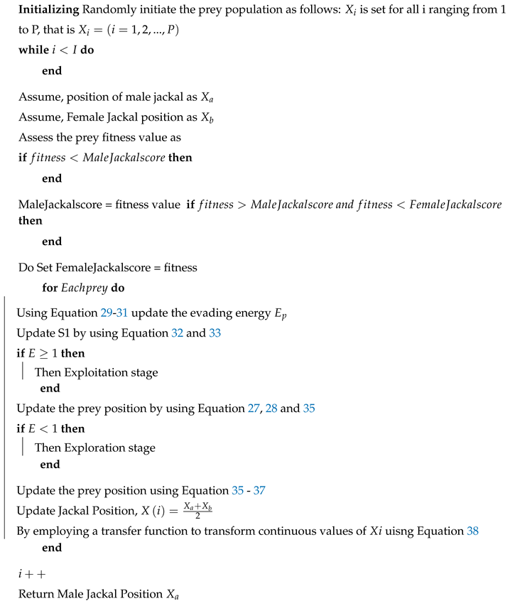 |
Figure 3.
Proposed algorithm GJO searching and attacking approches
The GJO approch, crafted as a metaheuristic optimization method inspired by the hunting behavior of golden jackals, initiates by randomly populating prey. It embarks on the pursuit of the best solution through multiple iterations, drawing parallels with jackals. In this analogy, the male jackal symbolizes the currently best solution, and the second-best choice is symbolized by the female jackal. The algorithm subsequently fine-tunes the location and evasive energy of every target by employing specific equations designed for the purpose. Subsequently, it proceeds with either exploration or exploitation based on the evasion energy value. The algorithm alters the jackal’s position by calculating the mean of the male and female locations. Subsequently, it converts the ongoing prey position values into binary equivalents through a specified transformation function. This repetitive procedure persists for a pre-defined number of iterations, ultimately yielding the male jackal’s position, which represents the optimal outcome achieved throughout its execution. This process serves to provide a deeper insight into the GJO algorithm, based on Algorithm 3 for a detailed explanation and Figure 4 for a visual depiction in a flowchart.
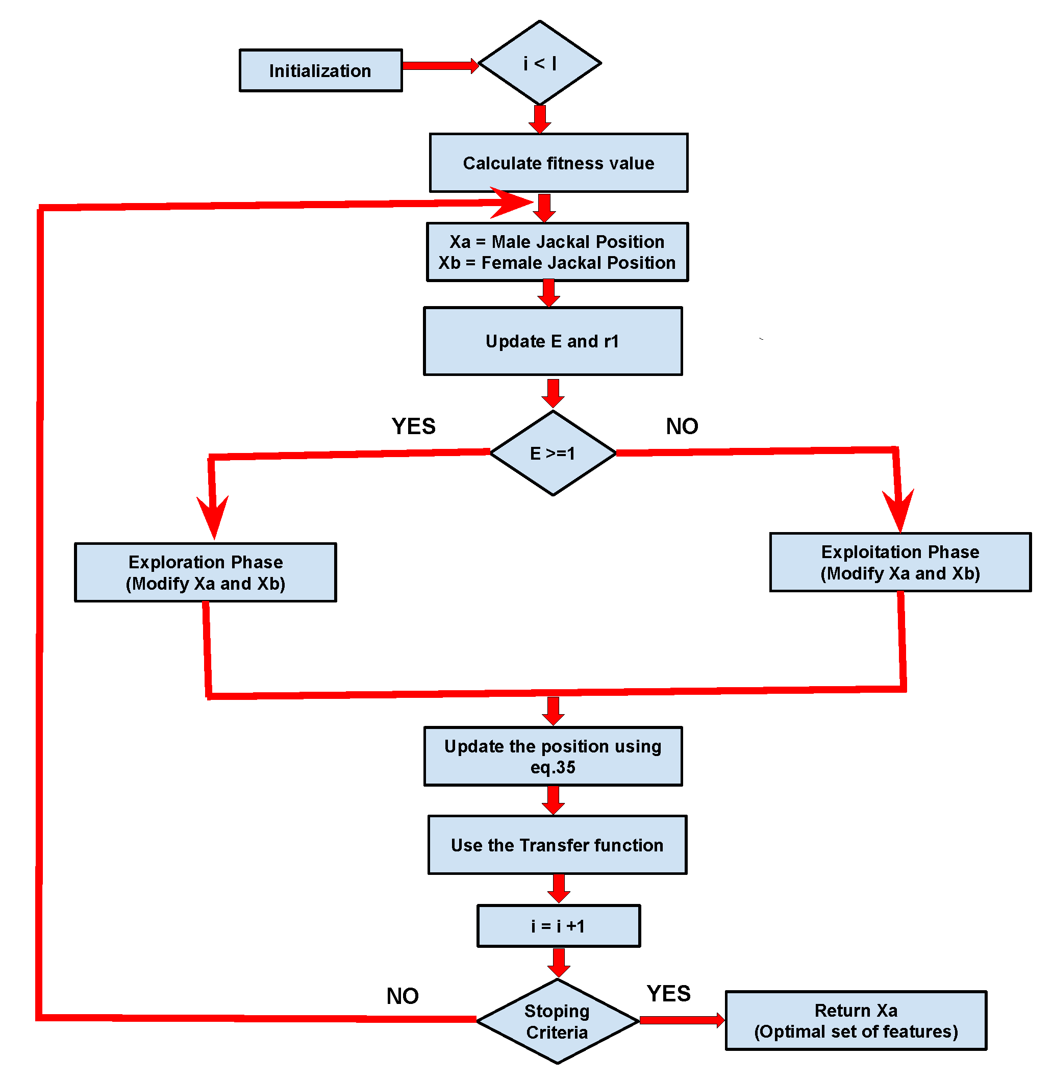
Figure 4.
Flowchart of the proposed algorithm
| Algorithm 3:Pseudocode of the proposed system |
 |
3.4. Classification using LS-SVM
In fundus image classification, machine learning classifiers are used to label data, a crucial aspect of supervised learning. There are several classifiers like XGBoost [41], random forest (RF) [8], decision trees (DT) [42], k-nearest neighbour (KNN) [5], and back-propagation neural network (BPNN) [5] with distinct applications and performance characteristics. In our proposed work, we have used LS-SVM to classify glaucoma fundus images.
Conventional SVM poses a substantial computational burden when handling large-dimensional datasets. To address this computational complexity, this paper employs a updated variant known as the least squares support vector machine (LS-SVM) has been used for glaucoma detection. Unlike the standard SVM, which involves solving a quadratic programming problem, LS-SVM operates by addressing a collection of linear equations because it uses equality constraints in its formulation [43]. In Equation 41, provided with a training dataset consisting of N data points represented as for k ranging from 1 to N, where each belongs to a space of dimension m and each is a class label taking values from, Formulating LS-SVM as an optimization problem can be expressed as follows:
Hence, the quality constant defined as follows
In Equation 42, specified as weight vector shown as mapping method, called the factor of regularization, b assigned as the bias and specifed as variables error. The Lagrangian can be specified as
Here, is specified as multipliers language. The optimality conditions in Equation 43 shown as , that specified as result of the following set of linear equations.
Here, . We have find the result as
Here, and based on Mercer’s condition [44],
Hence, is the kernel function. The LS-SVM algorithm can be obtained based on:
The kernel functions applied to train the classifier are tabulated in Table 3. The hyperparameter shows the degree of the polynomial, and is the free parameter that manages the shape of the kernel.

Table 2.
Several Kernel Functions applied in LS-SVM
| Kernel | Defination |
|---|---|
| Linear | |
| Polynomial | |
| Radial Basis Function (RBF) |
4. Experimental Results and Discussion
The experiments have been performed on the PARAM Shavak – Supercomputer with an HPC system set up in a tabletop configuration. This system has an Intel(R) Xeon(R) Gold 5220R CPU running at 2.20GHz. It boasts a minimum of 2 multicore CPUs, each possessing at least 12 cores, along with one or two GPU accelerator cards, including the NVIDIA K40 accelerator card and NVIDIA P5000. The system offers a computing power of 3 Tera-Flops at its peak, complemented by 8 TB of storage and 64 GB of RAM. It comes pre-loaded with a parallel programming development environment and possesses computing power of 2 TF and above. We conducted our experiments using the computer-aided diagnosis (CAD) model we proposed and implemented using Python 3.9.6. In our deployed work, we have considered two standard datasets, namely, G1020 [25] and ORIGA [26]. Here, we have divided the glaucoma datasets into a 60:40 ratio for training and testing to achieve the highest level of accuracy. The experiments have been configured with specific parameters like set at 1.5, the population size is 30, and the values of maximum iteration is 200 tabulated in the Table 3. Similarly, the hyper-parameters lists used for various classifiers have been tabulated in Table 4. We’ve utilized a five-fold stratified cross-validation (SCV)approach to address overfitting concerns. This technique splits the dataset into five distinct subparts, observing that no overlapping occurs. Then, the scheme was trained on four subparts and evaluated on the remaining part. This process continues five times; each subpart is the evaluation set once. This method enhances the model’s performance more and avoids overfitting. The 5-fold SCV for a single run has been shown in Figure 5.
Table 3.
Parameters utlized in GJO feature selection models
| Parameters | Values |
|---|---|
| Population size | 30 |
| Maximum iteration | 200 |
| r (Random integer) | 0 to 1 |
| c1(Constant value), | 1.5 |
Table 4.
Hyperparameters for different classifiers
| Algorithms | Specifications | Parameters |
|---|---|---|
| XGBoost [41] | Learning rate | 0.3 |
| n-estimators | 100 | |
| Scale-pos-wirght | 1 | |
| Random Forest [8] | n-estimators | 100 |
| Criterion | Gini | |
| Min-impurity-decrease | 0 | |
| Number of folds | 5 | |
| Decision Tree [42] | Criterion | Gini |
| Max-features | 0,1 | |
| Min-sample-leaf | 1 | |
| Min-sample-split | 2 | |
| KNN [5] | Nearest neighbors(K) | 1 |
| Nearset neighbor search algorithm | Euclidean distance | |
| List of folds | 5 | |
| BPNN[5] | Learning rate, momentum | 0.001, 0.4 |
| Hidden neurons | 6 | |
| List of folds | 5 | |
| LS-SVM Linear[45] | Dimension space | -1, +1 |
| Kernel type | Linear | |
| List of folds | 5 | |
| LS-SVM Polynomial [45] | Order | 2 |
| Kernel type | Poly | |
| List of folds | 5 | |
| LS-SVM RBF [45] | , | [1-10] |
| Kernel type | RBF | |
| List of folds | 5 |
Poly-Polynomial, RBF-Radial basis function kernel
4.1. Preprocessing and feature extraction results
To enhance the contrast of the initial glaucoma fundus image, the CLAHE method is used, and its performance is influenced by the settings of its parameters. In this scenario, the initial fundus image is partitioned into 64 distinct contextual regions, with 256 bins and a clip limit of 0.01 have been selected. It’s important to highlight that a uniform distribution approach is applied to each region to achieve a consistent flat histogram shape. Subsequently, we apply the DR2T technique to each preprocessed image, extracting features as transform coefficients using a 2-level 1D DWT with the Haar wavelet is chosen as the basis because of its straightforward nature. Since the sum of glaucoma fundus images has been obtained, the dimensions of . Hence, instead of DR2T, we employ 2D DWT and ridglet transform, and we have preserved their coefficients. The procedure entails determining the magnitude of the coefficients for each change and then normalizing them according to the most crucial coefficient. The normalized coefficients’ magnitudes are then arranged in descending order to assess the rate of reduction in coefficients, as illustrated in Figure 6. Notably, DR2T outperforms 2D DWT and ridgelet regarding the speed at which coefficients decline. Consequently, DR2T generates sparse feature vectors that notably improve classification accuracy.
4.2. Feature selection results
Here, we have implemented a novel method for feature selection, which involves using the golden jackal optimization (GJO) algorithm. This approach leverages metaheuristic optimization with the GJO algorithm to effectively identify the most optimal set of features, i.e., (29 features) from discrete ripplet-II transform (DR2T). Feature selection helps mitigate collinearity, leading to more stable coefficient estimates and improved model accuracy. From our experimental analysis, we have obtained better classification results on both datasets, namely, G1020 [25] and ORIGA [26] by selecting 29 number of features. The proposed model DR2T+GJO+LS-SVM+RBF provides better classification accuracy with 29 optimal features. Also, we have compared the performance of our proposed model with feature selection and without feature selection. The comparative analysis of the table is shown in Table 6. Similarly, we have compared the number of features with their respective classification accuracy, and the comparison graphs have been shown in Figure 7 and Figure 8. From the experimental results, we have observed that the proposed model DR2T+GJO+LS-SVM+RBF gives better classification accuracy with 29 optimal features in both datasets.
Table 5.
Comparative analyses (%) of the proposed model with LS-SVM with list of kernels and LS-SVM with kernels+GJO scheme
Table 5.
Comparative analyses (%) of the proposed model with LS-SVM with list of kernels and LS-SVM with kernels+GJO scheme
| Proposed Method | No. of feature |
G1020 | ORIGA | ||||
|---|---|---|---|---|---|---|---|
| DR2T+LS-SVM+Linear | 32 | 91.42 | 88.14 | 92.76 | 94.62 | 94.03 | 94.82 |
| DR2T+LS-SVM+Polynomial | 32 | 92.16 | 88.98 | 93.45 | 95.38 | 91.04 | 96.89 |
| DR2T+LS-SVM+RBF | 32 | 92.65 | 91.53 | 93.10 | 96.15 | 94.03 | 96.89 |
| DR2T+GJO+LS-SVM+Linear | 29 | 92.63 | 90.60 | 93.45 | 95.77 | 95.52 | 95.82 |
| DR2T+GJO+LS-SVM+Polynomial | 29 | 93.14 | 90.68 | 94.14 | 96.54 | 96.37 | 97.01 |
| DR2T+GJO+LS-SVM+RBF | 29 | 93.38 | 92.37 | 93.79 | 97.31 | 97.01 | 97.41 |
| -Accuracy, -Sensitivity, -Specificity | |||||||
4.3. Classification results
We have utilized LS-SVM with several kernels for glaucoma detection during our classification. We have assessed how well our suggested model performs using three parameters: accuracy, sensitivity and specificity. Here, we have considered two standard datasets: G1020 [25] and ORIGA [26]. To improve the quality of our dataset, we applied a cropping process to extract relevant regions of interest (ROI). Ophthalmologists provided the cup and disc values on numerous images. Our approach primarily centred on cropped images resized at 256 × 256 pixels. In cases where specific ROIs were unavailable due to a lack of prior knowledge, the entire 256 × 256 image has been considered. We have divided our whole dataset into training and testing with the ratio 60:40. The training and testing samples details have been specified in Table , and some samples of the dataset set have been shown in Figure . We have deployed by assessing the classification performance through a 5-fold stratified cross-validation procedure involving ten iterations and manually fine-tuned the model’s hyperparameters to extract high-level features. Then, the LS-SVM has been the prime classifier in our classification task. We have used different traditional classifiers like XGBoost [41], RF [8], DT [42], KNN [5], and BPNN [5] with accuracy 90.93%, 89.22%, 88.97%, 91.18%, 91.67% accordingly in the G1020 dataset. Similarly, in the ORIGA dataset, several classifiers, namely, XGBosst, RF, DT, KNN, and BPNN, have an accuracy of 91.41%, 90.63%, 89.84%, 93.44%, 93.46%. The comparison of all existing classifiers with our deployed scheme is tabulated in Table 6. Furthermore, to showcase the enhanced performance of DR2T features in comparison to DWT and curvelet (FDCT) features, we carried out an experiment in which we separately utilized DWT and FDCT features within the proposed system, and the outcomes can be found in Table 7. From the classification results, we have observed that our suggested model produced superior classification accuracy at 93.38% and 97.31% with the G1020 and ORIGA datasets, respectively. Table 8 to Table 11 represents the details of 5-fold SCV results of both the datasets. The AUC results of different kernels obtained by the false positive rate concerning the true positive rate on both the G1020 and ORIGA datasets are shown in Figure 9 and Figure 10. Then, The confusion matrix of both datasets, namely G1020 and ORIGA, is shown in Figure 11. The performance comparison of the various classifiers on both datasets has been shown in Figure 12 and Figure 13, respectively.
Table 6.
Comparative analysis (%) of deployed model with Glaucoma datasets
| Classifiers | G1020 Dataset | ORIGA Dataset | ||||
|---|---|---|---|---|---|---|
| XGBoost | 90.93 | 87.29 | 92.41 | 91.41 | 88.89 | 92.23 |
| RF | 89.22 | 83.90 | 91.38 | 90.63 | 87.38 | 91.71 |
| DT | 88.97 | 86.97 | 90.00 | 89.84 | 85.84 | 91.19 |
| KNN | 91.18 | 87.29 | 92.76 | 93.44 | 92.54 | 93.75 |
| BPNN | 91.67 | 89.83 | 92.41 | 93.46 | 89.55 | 94.82 |
| DR2T+GJO+LS-SVM+RBF(Proposed) | 93.38 | 92.37 | 93.79 | 97.31 | 97.01 | 97.41 |
| : Accuracy, : Sensitivity , : Specificity | ||||||
Table 7.
Comparative result(%) based on wavelet and curvlet based on G1020 and ORIGA dataset
| Schemes | No. of features | Dataset ( in (%) | |
| G1020 | ORIGA | ||
| DWT+LS-SVM | 32 | 90.20 | 91.92 |
| DWT+GJO+LS-SVM | 32 | 91.42 | 94.23 |
| FDCT+GJO+LS-SVM | 32 | 91.98 | 95.38 |
| DR2T+GJO+LS-SVM | 29 | 93.38 | 97.31 |
Table 8.
Glaucoma detection of average results (%) of suggested DR2T without GJO architecture for G1020 dataset for 5-fold 10 times for DR2T+LS-SVM+RBF kernel
Table 8.
Glaucoma detection of average results (%) of suggested DR2T without GJO architecture for G1020 dataset for 5-fold 10 times for DR2T+LS-SVM+RBF kernel
| R | ||||||
|---|---|---|---|---|---|---|
| 1 | 92.65 | 92.65 | 92.65 | 92.63 | 92.63 | 92.64 |
| 2 | 92.65 | 92.65 | 92.65 | 92.65 | 92.63 | 92.65 |
| 3 | 92.65 | 92.65 | 92.65 | 92.63 | 92.63 | 92.64 |
| 4 | 92.65 | 92.65 | 92.65 | 92.65 | 92.63 | 92.65 |
| 5 | 92.65 | 92.65 | 92.65 | 92.63 | 92.65 | 92.65 |
| 6 | 92.65 | 92.65 | 92.63 | 93.65 | 93.65 | 92.65 |
| 7 | 92.65 | 92.65 | 92.63 | 92.63 | 92.63 | 92.64 |
| 8 | 92.65 | 92.65 | 92.65 | 92.65 | 92.63 | 92.65 |
| 9 | 92.65 | 92.65 | 92.65 | 92.65 | 92.63 | 92.65 |
| 10 | 92.65 | 92.65 | 92.65 | 92.63 | 92.65 | 92.65 |
| Final Result | 92.65 ± 0.0045 | |||||
| : Fold Number, R: Run, : Average Accuracy | ||||||
Table 9.
Glaucoma detection of average results (%) of suggested DR2T with GJO architecture for G1020 dataset for 5-fold 10 times for DR2T+GJO+LS-SVM+RBF kernel
Table 9.
Glaucoma detection of average results (%) of suggested DR2T with GJO architecture for G1020 dataset for 5-fold 10 times for DR2T+GJO+LS-SVM+RBF kernel
| R | ||||||
|---|---|---|---|---|---|---|
| 1 | 93.30 | 93.30 | 93.30 | 93.63 | 93.63 | 93.43 |
| 2 | 93.30 | 93.30 | 93.30 | 93.63 | 93.63 | 93.43 |
| 3 | 93.30 | 93.30 | 93.30 | 93.3 | 93.3 | 93.30 |
| 4 | 93.30 | 93.30 | 93.30 | 93.63 | 93.63 | 93.43 |
| 5 | 93.30 | 93.30 | 93.30 | 93.63 | 93.63 | 93.43 |
| 6 | 93.30 | 93.30 | 93.30 | 93.30 | 93.30 | 93.30 |
| 7 | 93.30 | 93.30 | 93.30 | 93.63 | 93.63 | 93.43 |
| 8 | 93.30 | 93.30 | 93.30 | 93.30 | 93.30 | 93.30 |
| 9 | 93.30 | 93.30 | 93.30 | 93.63 | 93.63 | 93.43 |
| 10 | 93.30 | 93.30 | 93.30 | 93.30 | 93.30 | 93.30 |
| Final Result | 93.38 ± 0.0636 | |||||
| : Fold Number, R: Run, : Average Accuracy | ||||||
Table 10.
Glaucoma detection of average results (%) of suggested DR2T without GJO architecture for ORIGA dataset for 5-fold 10 times for LS-SVM+RBF kernel
Table 10.
Glaucoma detection of average results (%) of suggested DR2T without GJO architecture for ORIGA dataset for 5-fold 10 times for LS-SVM+RBF kernel
| R | ||||||
|---|---|---|---|---|---|---|
| 1 | 96.03 | 96.03 | 96.27 | 96.27 | 96.27 | 96.17 |
| 2 | 96.03 | 96.03 | 96.27 | 96.27 | 96.27 | 96.17 |
| 3 | 96.03 | 96.03 | 96.03 | 96.03 | 96.27 | 96.08 |
| 4 | 96.27 | 96.27 | 96.27 | 96.03 | 96.03 | 96.17 |
| 5 | 96.03 | 96.03 | 96.27 | 96.27 | 96.27 | 96.17 |
| 6 | 96.03 | 96.03 | 96.03 | 96.03 | 96.27 | 96.08 |
| 7 | 96.03 | 96.03 | 96.27 | 96.27 | 96.27 | 96.17 |
| 8 | 96.27 | 96.27 | 96.27 | 96.03 | 96.03 | 96.17 |
| 9 | 96.03 | 96.03 | 96.27 | 96.27 | 96.27 | 96.17 |
| 10 | 96.03 | 96.03 | 96.03 | 96.03 | 96.27 | 96.08 |
| Final Result | 96.15 ± 0.0017 | |||||
| : Fold Number, R: Run, : Average Accuracy | ||||||
Table 11.
Glaucoma detection of average results (%) of suggested DR2T with GJO architecture for ORIGA dataset for 5-fold 10 times for DR2T+GJO+LS-SVM+RBF kernel
Table 11.
Glaucoma detection of average results (%) of suggested DR2T with GJO architecture for ORIGA dataset for 5-fold 10 times for DR2T+GJO+LS-SVM+RBF kernel
| R | ||||||
|---|---|---|---|---|---|---|
| 1 | 97.31 | 97.30 | 97.31 | 97.31 | 97.31 | 97.31 |
| 2 | 97.31 | 97.30 | 97.31 | 97.31 | 97.31 | 97.31 |
| 3 | 97.30 | 97.30 | 97.30 | 97.30 | 97.30 | 97.30 |
| 4 | 97.31 | 97.31 | 97.31 | 97.31 | 97.31 | 97.31 |
| 5 | 97.31 | 97.31 | 97.31 | 97.31 | 97.31 | 97.31 |
| 6 | 97.30 | 97.30 | 97.30 | 97.30 | 97.30 | 97.30 |
| 7 | 97.31 | 97.31 | 97.31 | 97.31 | 97.31 | 97.31 |
| 8 | 97.31 | 97.31 | 97.30 | 97.31 | 97.31 | 97.31 |
| 9 | 97.31 | 97.31 | 97.30 | 97.31 | 97.31 | 97.31 |
| 10 | 97.30 | 97.30 | 97.30 | 97.30 | 97.30 | 97.30 |
| Final Result | 97.31 ± 0.0045 | |||||
| : Fold Number, R: Run, : Average Accuracy | ||||||
4.4. Compariosn with other state-of-the-art models
We have conducted experiments to evaluate our new model, comparing it to previous models. To gauge its effectiveness, we have compared our proposed model with traditional CAD schemes. The results of this evaluation, conducted with G1020 and ORIGA images, are displayed in Table 12. Our proposed model obtained better classification outcomes than existing models, even with fewer features. This represents a significant advantage compared to various CAD models for identifying glaucoma. While the increase in accuracy is modest and similar to specific existing methods, it’s worth noting that this outcome was achieved across multiple iterations of a k-fold stratified cross-validation procedure, underscoring the robustness and dependability of the proposed approach.
Table 12.
Performance analysis of proposed model with existing CAD models with G1020 and ORIGA datasets
Table 12.
Performance analysis of proposed model with existing CAD models with G1020 and ORIGA datasets
| Existing Methods | (%) | |
|---|---|---|
| Datasets | ||
| G1020 | ORIGA | |
| 2D-FBSE-EWT [46] | — | 91.01 |
| SMOTE+RF [47] | — | 78.30 |
| SMOTE+SVM [47] | — | 82.80 |
| HOG+SVM [48] | 83.32 | — |
| HOG +PNN [48] | 87.92 | — |
| HOG+RNN [48] | 85.72 | — |
| DR2T+GJO+LS-SVM+RBF(Proposed Model) | 93.38 | 97.31 |
| - Accuracy | ||
4.5. Advantages and Disadvantages of Proposed Model
The experimental results show that the proposed model improves the classification results as compared to other existing models with less number of features. The proposed model uses discrete ripplet-II transform (DR2T) for feature extraction. Compared to other transforms like discrete wavelet transform (DWT), Fourier transform, ridgelet, lifting wavelet transform (LWT), etc., DR2T has produced 2D singularities with arbitrarily shaped curves, which are available in the fundus images. Also, it provides rotation invariant and sparse features, which is important for improving the classification problem. Here, the golden Jackel optimization (GJO) algorithm has been used to select the optimal features with reduced feature dimensions and improve the model’s accuracy.
Still, the proposed model has several demerits, as follows. The proposed model has been experimented with only retinal fundus images. We can test our model with other images like Optical Coherence Tomography (OCT) images, Confocal Scanning Laser Ophthalmoscopy (CSLO) images, etc. The proposed model solves binary classification problems, but multiclass classification is challenging. However, the GJO requires more number of parameters to tune, so in future, we can use other optimisation techniques with less number of parameters.
5. Conclusions and Future Scope
The paper introduced an improved glaucoma detection model, which uses ripplet-II transform (DR2T) to extract the relevant features from the enhanced fundus images. A meta-heuristic optimization algorithm called golden jackal optimization (GJO) has been employed for selecting the optimal features to reduce the dimension of the feature vector. Finally, LS-SVM with RBF kernel applied to classify the image as glaucoma or healthy. The proposed model represents the advantages of DR2T and GJO for glaucoma detection from fundus images. The findings from the experiments on two recognized datasets show that the suggested method achieves greater classification accuracy than other competent methods, even when using a minimal number of features. In the future, the proposed model’s overall performance could be enhanced by employing advanced feature extraction and selection techniques. Deep learning could be investigated as a vital alternative to the deployed scheme, and hybridizing fewer parameters based on different optimization techniques can be another future work.
Author Contributions
Conceptualization, S.S. and D.M.; methodology, S.S. and D.M.; software, S.S., D.M. and G.P; validation, D.M, G.P,and S.D; formal analysis, S.S., D.M. and A.R; investigation, S.S. and D.M.; resources, S.S. and D.M.; data curation, X.X.; writing—original draft preparation, S.S. and D.M.; writing—review and editing, S.S., D.M., G.P. and S.D; visualization,S.S., D.M., G.P. and S.D ; supervision, D.M., G.P. and S.D; project administration, D.M., G.P. and S.D; funding acquisition, S.D. All authors have read and agreed to the published version of the manuscript.
Funding
This research received no external funding
Conflicts of Interest
The authors declare no conflict of interest.
References
- Singh, A.; Dutta, M.K.; ParthaSarathi, M.; Uher, V.; Burget, R. Image processing based automatic diagnosis of glaucoma using wavelet features of segmented optic disc from fundus image. Computer methods and programs in biomedicine 2016, 124, 108–120. [Google Scholar] [CrossRef] [PubMed]
- Drance, S.; Anderson, D.R.; Schulzer, M.; Group, C.N.T.G.S.; others. Risk factors for progression of visual field abnormalities in normal-tension glaucoma. American journal of ophthalmology 2001, 131, 699–708. [Google Scholar] [CrossRef]
- Fu, H.; Cheng, J.; Xu, Y.; Zhang, C.; Wong, D.W.K.; Liu, J.; Cao, X. Disc-aware ensemble network for glaucoma screening from fundus image. IEEE transactions on medical imaging 2018, 37, 2493–2501. [Google Scholar] [CrossRef]
- Garway-Heath, D.; Hitchings, R. Quantitative evaluation of the optic nerve head in early glaucoma. British Journal of Ophthalmology 1998, 82, 352–361. [Google Scholar] [CrossRef]
- Muduli, D.; Dash, R.; Majhi, B. Automated breast cancer detection in digital mammograms: A moth flame optimization based ELM approach. Biomedical Signal Processing and Control 2020, 59, 101912. [Google Scholar] [CrossRef]
- Muduli, D.; Dash, R.; Majhi, B. Automated diagnosis of breast cancer using multi-modal datasets: A deep convolution neural network based approach. Biomedical Signal Processing and Control 2022, 71, 102825. [Google Scholar] [CrossRef]
- Muduli, D.; Dash, R.; Majhi, B. Fast discrete curvelet transform and modified PSO based improved evolutionary extreme learning machine for breast cancer detection. Biomedical Signal Processing and Control 2021, 70, 102919. [Google Scholar] [CrossRef]
- Muduli, D.; Priyadarshini, R.; Barik, R.C.; Nanda, S.K.; Barik, R.K.; Roy, D.S. Automated Diagnosis of Breast Cancer using Combined Features and Random Forest Classifier. 2023 6th International Conference on Information Systems and Computer Networks (ISCON). IEEE, 2023, pp. 1–4.
- Muduli, D.; Dash, R.; Majhi, B. Enhancement of Deep Learning in Image Classification Performance Using VGG16 with Swish Activation Function for Breast Cancer Detection. Computer Vision and Image Processing: 5th International Conference, CVIP 2020, Prayagraj, India, December 4-6, 2020, Revised Selected Papers, Part I 5. Springer, 2021, pp. 191–199.
- Muduli, D.; Kumar, R.R.; Pradhan, J.; Kumar, A. An empirical evaluation of extreme learning machine uncertainty quantification for automated breast cancer detection. Neural Computing and Applications, 2023, pp. 1–16.
- Sharma, S.K.; Zamani, A.T.; Abdelsalam, A.; Muduli, D.; Alabrah, A.A.; Parveen, N.; Alanazi, S.M. A Diabetes Monitoring System and Health-Medical Service Composition Model in Cloud Environment. IEEE Access 2023, 11, 32804–32819. [Google Scholar] [CrossRef]
- Sharma, S.K.; Priyadarshi, A.; Mohapatra, S.K.; Pradhan, J.; Sarangi, P.K. Comparative Analysis of Different Classifiers Using Machine Learning Algorithm for Diabetes Mellitus. In Meta Heuristic Techniques in Software Engineering and Its Applications: METASOFT 2022; Springer, 2022; pp. 32–42.
- Yin, F.; Lee, B.H.; Yow, A.P.; Quan, Y.; Wong, D.W.K. Automatic ocular disease screening and monitoring using a hybrid cloud system. 2016 IEEE international conference on Internet of Things (iThings) and IEEE green computing and communications (GreenCom) and IEEE cyber, physical and social computing (CPSCom) and IEEE smart data (SmartData). IEEE, 2016, pp. 263–268.
- Islam, M.T.; Imran, S.A.; Arefeen, A.; Hasan, M.; Shahnaz, C. Source and camera independent ophthalmic disease recognition from fundus image using neural network. 2019 IEEE International Conference on Signal Processing, Information, Communication & Systems (SPICSCON). IEEE, 2019, pp. 59–63.
- Maheshwari, S.; Pachori, R.B.; Acharya, U.R. Automated diagnosis of glaucoma using empirical wavelet transform and correntropy features extracted from fundus images. IEEE journal of biomedical and health informatics 2016, 21, 803–813. [Google Scholar] [CrossRef]
- Maheshwari, S.; Pachori, R.B.; Kanhangad, V.; Bhandary, S.V.; Acharya, U.R. Iterative variational mode decomposition based automated detection of glaucoma using fundus images. Computers in biology and medicine 2017, 88, 142–149. [Google Scholar] [CrossRef]
- Kausu, T.; Gopi, V.P.; Wahid, K.A.; Doma, W.; Niwas, S.I. Combination of clinical and multiresolution features for glaucoma detection and its classification using fundus images. Biocybernetics and Biomedical Engineering 2018, 38, 329–341. [Google Scholar] [CrossRef]
- Raghavendra, U.; Bhandary, S.V.; Gudigar, A.; Acharya, U.R. Novel expert system for glaucoma identification using non-parametric spatial envelope energy spectrum with fundus images. Biocybernetics and Biomedical Engineering 2018, 38, 170–180. [Google Scholar] [CrossRef]
- Parashar, D.; Agrawal, D.K.; Tyagi, P.K.; Rathore, N. Automated Glaucoma Classification Using Advanced Image Decomposition Techniques From Retinal Fundus Images. In AI-Enabled Smart Healthcare Using Biomedical Signals; IGI Global, 2022; pp. 240–258.
- Wang, W.; Zhou, W.; Ji, J.; Yang, J.; Guo, W.; Gong, Z.; Yi, Y.; Wang, J. Deep sparse autoencoder integrated with three-stage framework for glaucoma diagnosis. International Journal of Intelligent Systems 2022, 37, 7944–7967. [Google Scholar] [CrossRef]
- Shyla, N.J.; Emmanuel, W.S. Automated classification of glaucoma using DWT and HOG features with extreme learning machine. 2021 third international conference on intelligent communication technologies and virtual mobile networks (ICICV). IEEE, 2021, pp. 725–730.
- Balasubramanian, K.; N. P., A. Correlation-based feature selection using bio-inspired algorithms and optimized KELM classifier for glaucoma diagnosis. Applied Soft Computing 2022, 128, 109432. [Google Scholar] [CrossRef]
- Latif, J.; Tu, S.; Xiao, C.; Bilal, A.; Ur Rehman, S.; Ahmad, Z. Enhanced Nature Inspired-Support Vector Machine for Glaucoma Detection. Computers, Materials & Continua 2023, 76. [Google Scholar]
- Raja, C.; Gangatharan, N. A hybrid swarm algorithm for optimizing glaucoma diagnosis. Computers in biology and medicine 2015, 63, 196–207. [Google Scholar] [CrossRef]
- Bajwa, M.N.; Singh, G.A.P.; Neumeier, W.; Malik, M.I.; Dengel, A.; Ahmed, S. G1020: A benchmark retinal fundus image dataset for computer-aided glaucoma detection. 2020 International Joint Conference on Neural Networks (IJCNN). IEEE, 2020, pp. 1–7.
- Zhang, Z.; Yin, F.S.; Liu, J.; Wong, W.K.; Tan, N.M.; Lee, B.H.; Cheng, J.; Wong, T.Y. Origa-light: An online retinal fundus image database for glaucoma analysis and research. 2010 Annual international conference of the IEEE engineering in medicine and biology. IEEE, 2010, pp. 3065–3068.
- Pizer, S.M. Contrast-limited adaptive histogram equalization: Speed and effectiveness stephen m. pizer, r. eugene johnston, james p. ericksen, bonnie c. yankaskas, keith e. muller medical image display research group. Proceedings of the first conference on visualization in biomedical computing, Atlanta, Georgia, 1990, Vol. 337, p. 2.
- Pisano, E.D.; Zong, S.; Hemminger, B.M.; DeLuca, M.; Johnston, R.E.; Muller, K.; Braeuning, M.P.; Pizer, S.M. Contrast limited adaptive histogram equalization image processing to improve the detection of simulated spiculations in dense mammograms. Journal of Digital imaging 1998, 11, 193–200. [Google Scholar] [CrossRef]
- Do, M.N.; Vetterli, M. The finite ridgelet transform for image representation. IEEE Transactions on image Processing 2003, 12, 16–28. [Google Scholar] [CrossRef] [PubMed]
- Candès, E.J.; Donoho, D.L. Ridgelets: A key to higher-dimensional intermittency? Philosophical Transactions of the Royal Society of London. Series A: Mathematical, Physical and Engineering Sciences 1999, 357, 2495–2509. [Google Scholar] [CrossRef]
- Candès, E.J.; Donoho, D.L. ; others. Curvelets: A surprisingly effective nonadaptive representation for objects with edges, Department of Statistics, Stanford University USA, 1999.
- Candes, E.; Demanet, L.; Donoho, D.; Ying, L. Fast discrete curvelet transforms. multiscale modeling & simulation 2006, 5, 861–899. [Google Scholar]
- Xu, J.; Yang, L.; Wu, D. Ripplet: A new transform for image processing. Journal of Visual Communication and Image Representation 2010, 21, 627–639. [Google Scholar] [CrossRef]
- Ghahremani, M.; Ghassemian, H. Remote sensing image fusion using ripplet transform and compressed sensing. IEEE Geoscience and Remote Sensing Letters 2014, 12, 502–506. [Google Scholar] [CrossRef]
- Xu, J.; Wu, D. Ripplet transform type II transform for feature extraction. IET Image processing 2012, 6, 374–385. [Google Scholar] [CrossRef]
- Cormack, A.M. The Radon transform on a family of curves in the plane. Proceedings of the American Mathematical Society 1981, 83, 325–330. [Google Scholar] [CrossRef]
- Cormack, A. The Radon transform on a family of curves in the plane. II. Proceedings of the American Mathematical Society 1982, 86, 293–298. [Google Scholar] [CrossRef]
- Kubecka, L.; Jan, J. Registration of bimodal retinal images-improving modifications. The 26th Annual International Conference of the IEEE Engineering in Medicine and Biology Society. IEEE, 2004, Vol. 1, pp. 1695–1698.
- Larabi-Marie-Sainte, S.; Alskireen, R.; Alhalawani, S. Emerging applications of bio-inspired algorithms in image segmentation. Electronics 2021, 10, 3116. [Google Scholar] [CrossRef]
- Das, H.; Prajapati, S.; Gourisaria, M.K.; Pattanayak, R.M.; Alameen, A.; Kolhar, M. Feature Selection Using Golden Jackal Optimization for Software Fault Prediction. Mathematics 2023, 11, 2438. [Google Scholar] [CrossRef]
- Raju, M.; Shanmugam, K.P.; Shyu, C.R. Application of Machine Learning Predictive Models for Early Detection of Glaucoma Using Real World Data. Applied Sciences 2023, 13, 2445. [Google Scholar] [CrossRef]
- Rodríguez-Robles, F.; Verdú-Monedero, R.; Berenguer-Vidal, R.; Morales-Sánchez, J.; Sellés-Navarro, I. Analysis of the Asymmetry between Both Eyes in Early Diagnosis of Glaucoma Combining Features Extracted from Retinal Images and OCTs into Classification Models. Sensors 2023, 23, 4737. [Google Scholar] [CrossRef]
- Nayak, D.R.; Dash, R.; Majhi, B. Least squares SVM approach for abnormal brain detection in MRI using multiresolution analysis. 2015 International Conference on Computing, Communication and Security (ICCCS). IEEE, 2015, pp. 1–6.
- Suykens, J.A.; Vandewalle, J. Least squares support vector machine classifiers. Neural processing letters 1999, 9, 293–300. [Google Scholar] [CrossRef]
- Kar, N.B.; Babu, K.S.; Sangaiah, A.K.; Bakshi, S. Face expression recognition system based on ripplet transform type II and least square SVM. Multimedia Tools and Applications 2019, 78, 4789–4812. [Google Scholar] [CrossRef]
- Chaudhary, P.K.; Pachori, R.B. Automatic diagnosis of glaucoma using two-dimensional Fourier-Bessel series expansion based empirical wavelet transform. Biomedical Signal Processing and Control 2021, 64, 102237. [Google Scholar] [CrossRef]
- Zhao, X.; Guo, F.; Mai, Y.; Tang, J.; Duan, X.; Zou, B.; Jiang, L. Glaucoma screening pipeline based on clinical measurements and hidden features. IET Image Processing 2019, 13, 2213–2223. [Google Scholar] [CrossRef]
- Ananya, S.; Bharamagoudra, M.R.; Bharath, K.; Pujari, R.R.; Hanamanal, V.A. Glaucoma Detection using HOG and Feed-forward Neural Network. 2023 IEEE International Conference on Integrated Circuits and Communication Systems (ICICACS). IEEE, 2023, pp. 1–5.
Figure 1.
Proposed CAD model for glaucoma classification
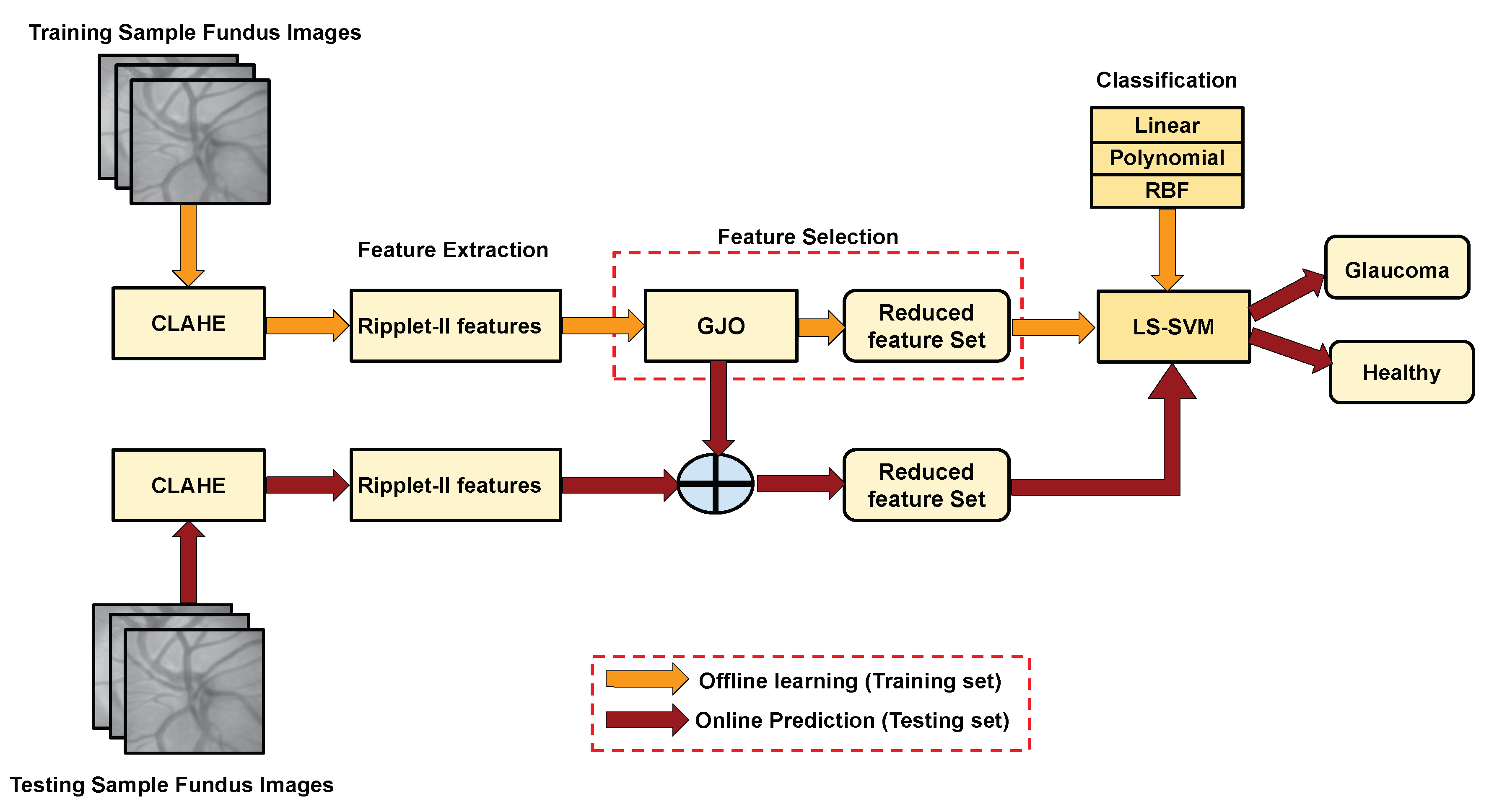
Figure 2.
Sample images of both datasets (G1020 and ORIGA).
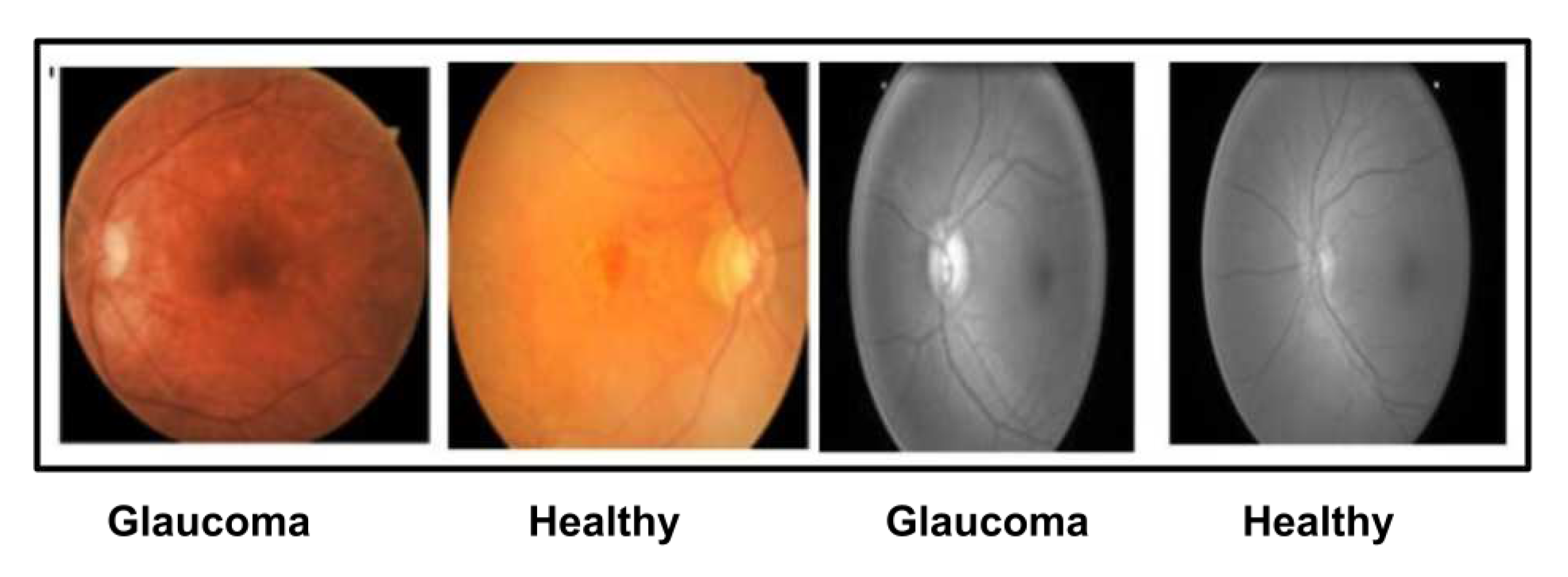
Figure 5.
Allocation of sample sets for each experiment through the utilization of k-Fold Stratified Cross-Validation
Figure 5.
Allocation of sample sets for each experiment through the utilization of k-Fold Stratified Cross-Validation
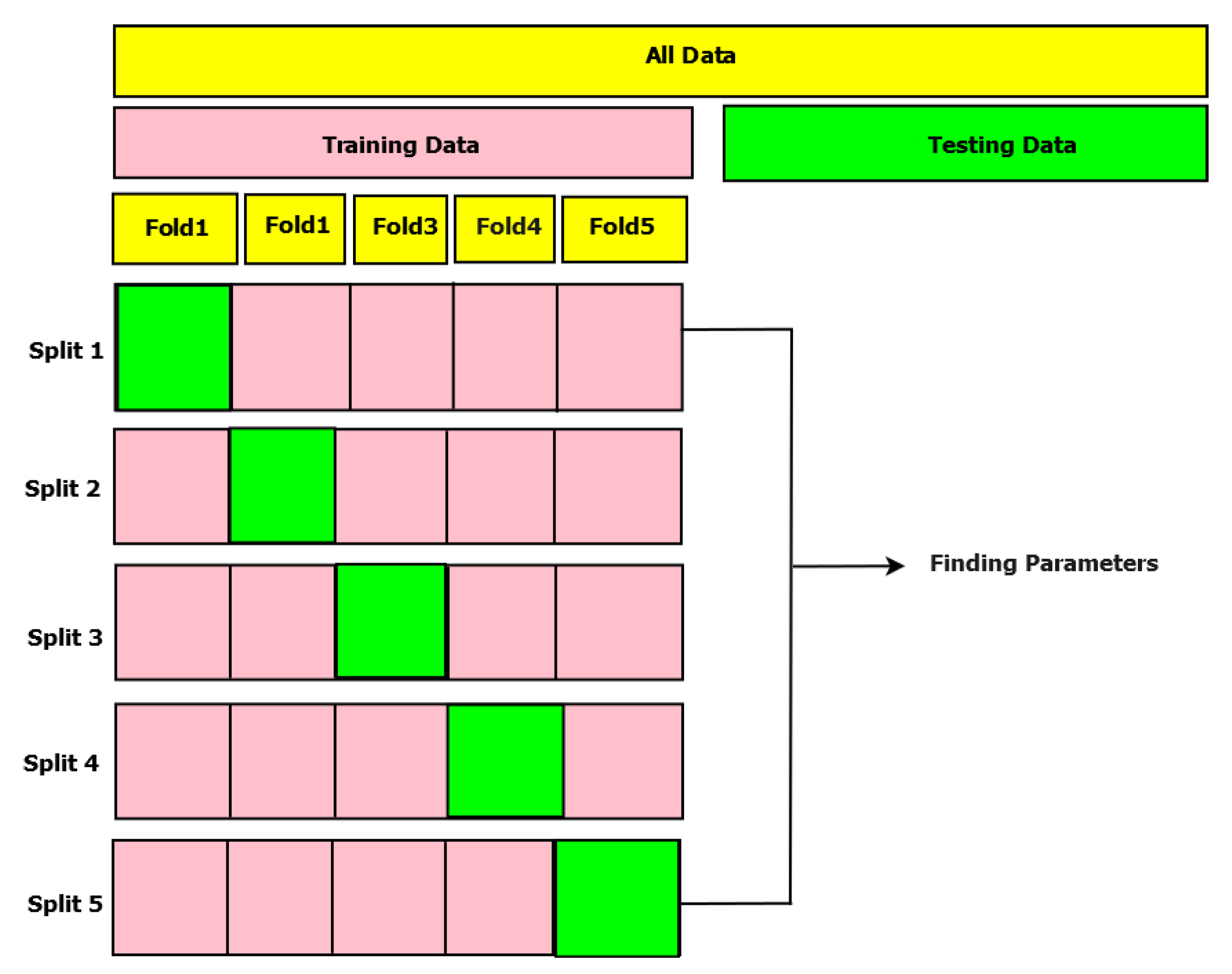
Figure 6.
Cofficient decaying comparision with list of image transform

Figure 7.
Classification result obtained in G1020 dataset has examined based on the number of features
Figure 7.
Classification result obtained in G1020 dataset has examined based on the number of features
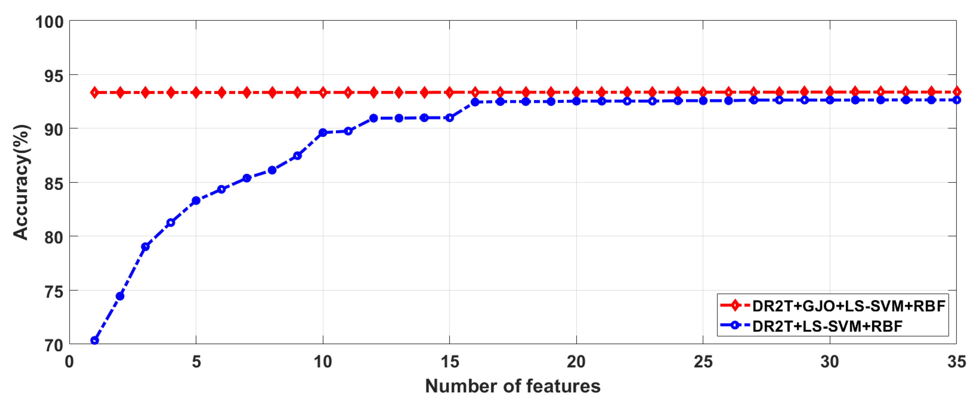
Figure 8.
Classification result obtained in ORIGA dataset has examined with based on the number of features
Figure 8.
Classification result obtained in ORIGA dataset has examined with based on the number of features
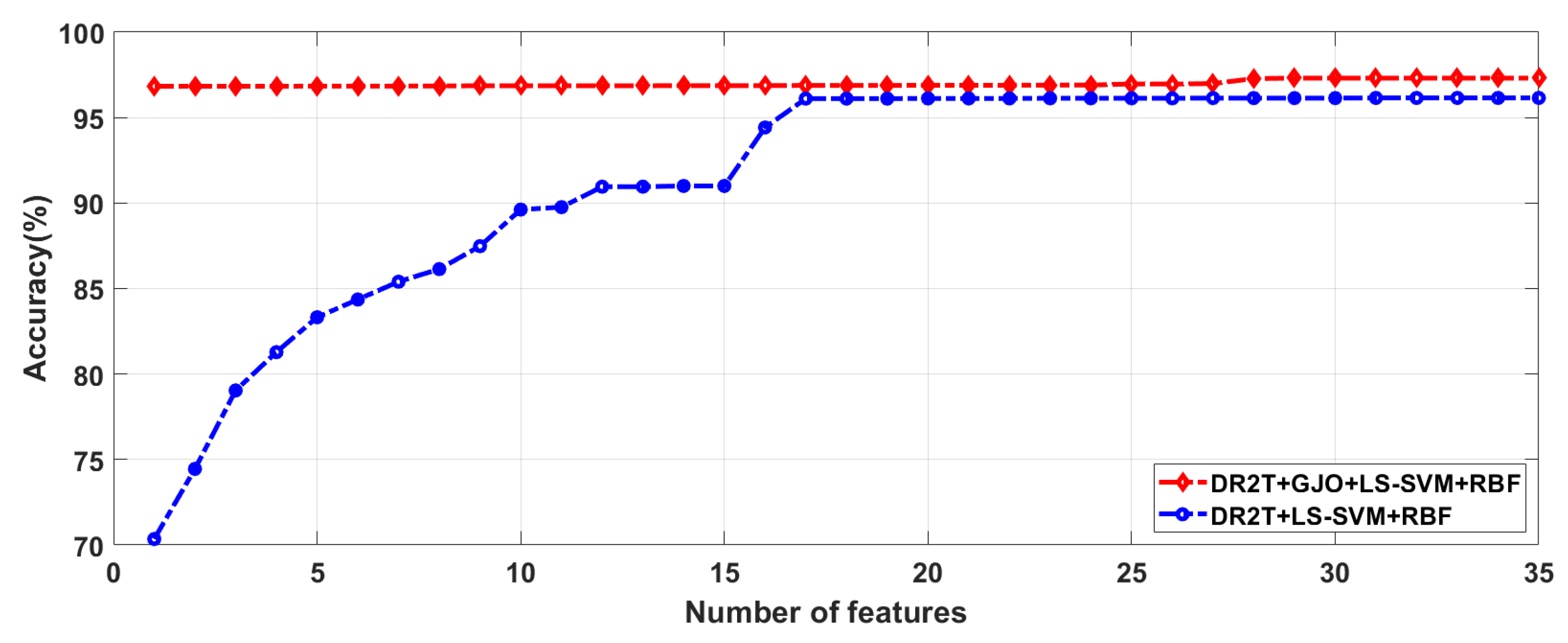
Figure 9.
The AUC curves for LS-SVM classifierwith three kernels using G1020 dataset
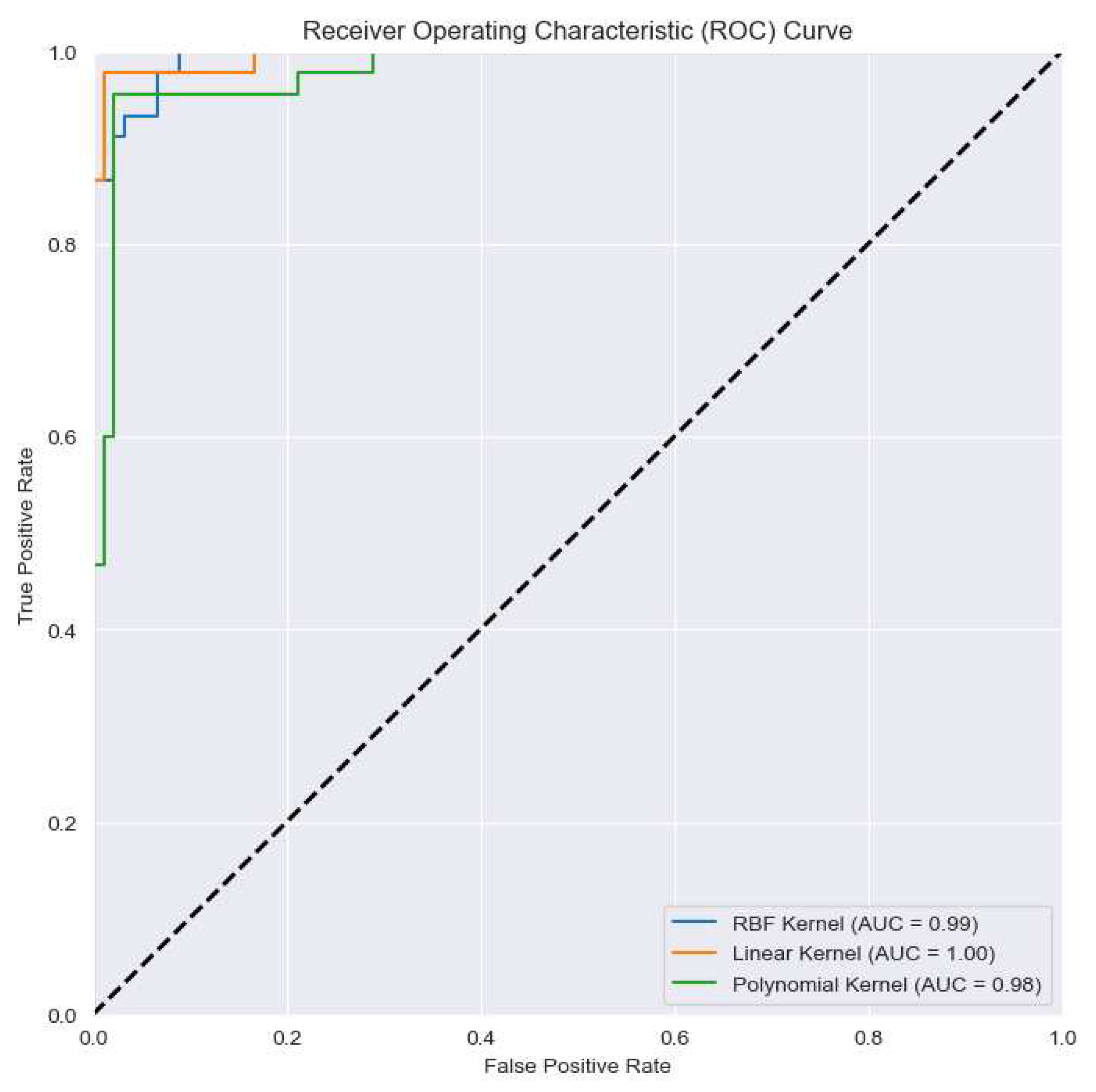
Figure 10.
The AUC curves for LS-SVM classifierwith three kernels using using ORIGA dataset
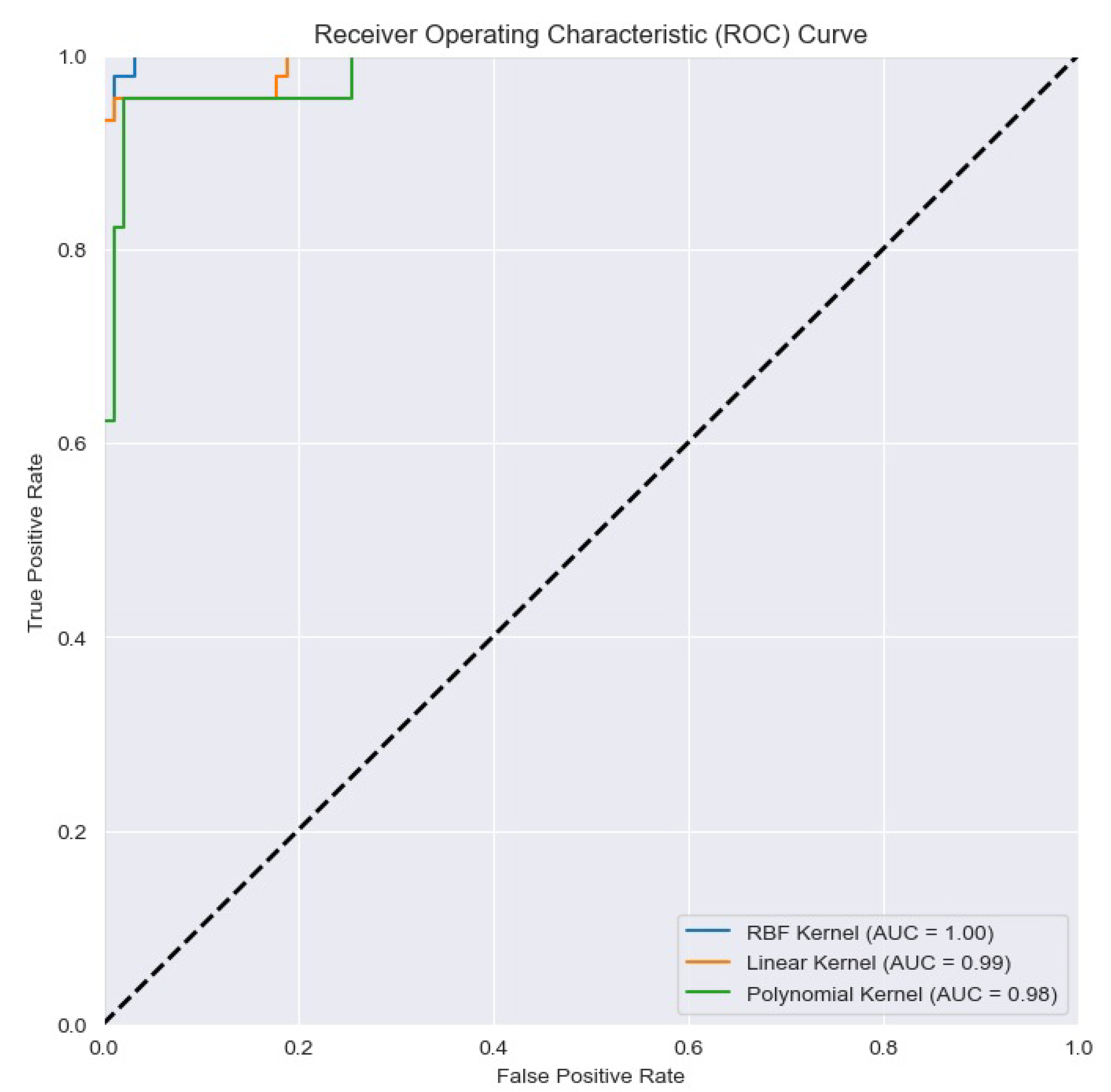
Figure 11.
Confusion matrix of proposed model visualized on G1020 and ORIGA Datasets
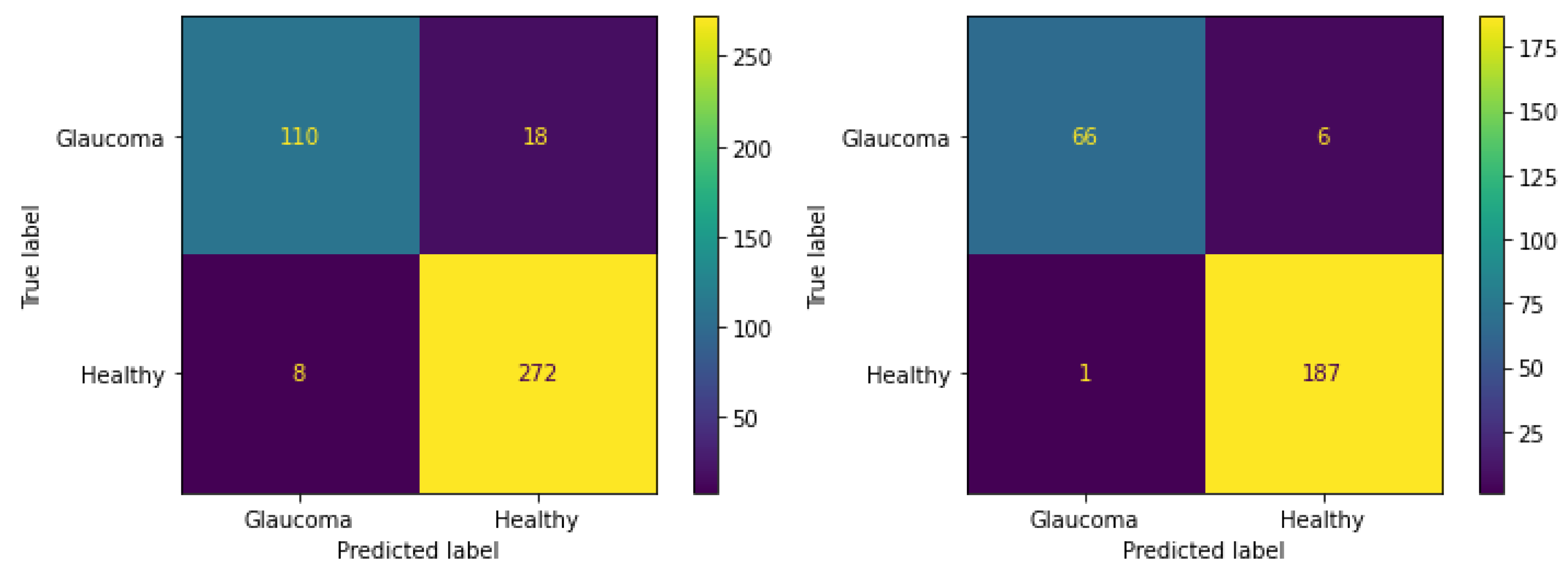
Figure 12.
Classification accuracy achieved by various classifiers with proposed scheme using G1020 dataset
Figure 12.
Classification accuracy achieved by various classifiers with proposed scheme using G1020 dataset
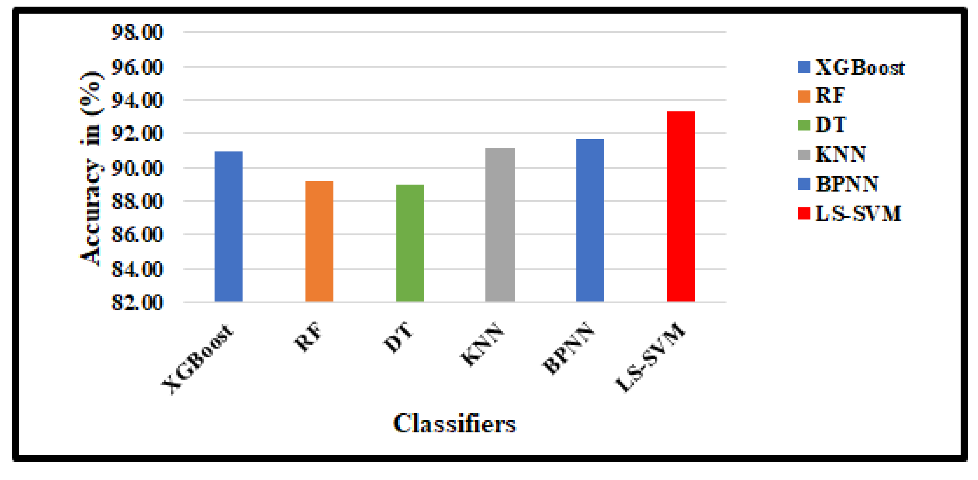
Figure 13.
Classification accuracy achieved by various classifiers with proposed scheme using ORIGA dataset
Figure 13.
Classification accuracy achieved by various classifiers with proposed scheme using ORIGA dataset
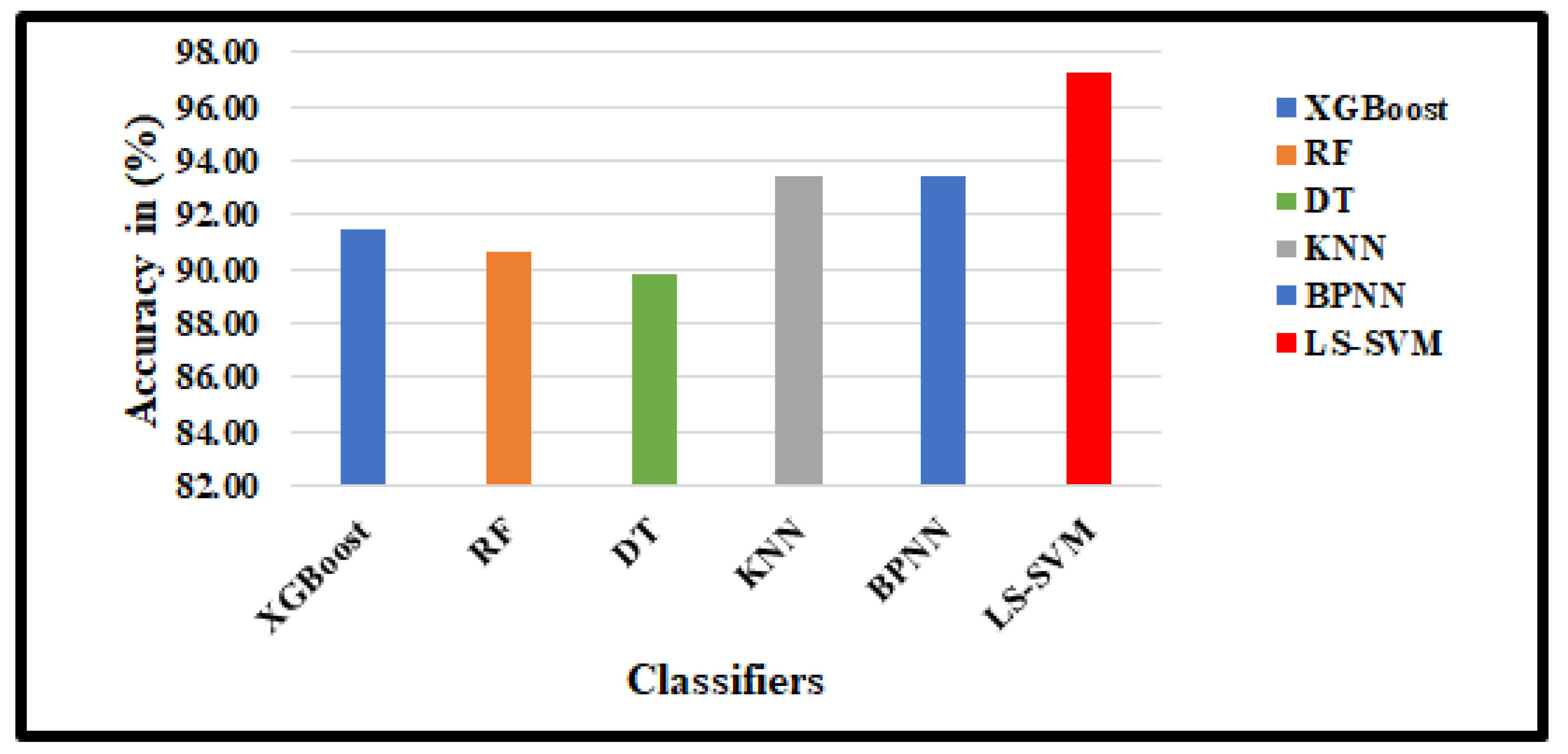
Table 1.
Proposed Glaucoma Data Sets(Glaucoma Vs. Healthy)
| Data sets | Total Images | Training Images | Testing Images | |||
|---|---|---|---|---|---|---|
| G | H | G | H | G | H | |
| G1020 | 296 | 724 | 178 | 434 | 118 | 290 |
| ORIGA | 168 | 482 | 101 | 289 | 67 | 193 |
Disclaimer/Publisher’s Note: The statements, opinions and data contained in all publications are solely those of the individual author(s) and contributor(s) and not of MDPI and/or the editor(s). MDPI and/or the editor(s) disclaim responsibility for any injury to people or property resulting from any ideas, methods, instructions or products referred to in the content. |
© 2023 by the authors. Licensee MDPI, Basel, Switzerland. This article is an open access article distributed under the terms and conditions of the Creative Commons Attribution (CC BY) license (http://creativecommons.org/licenses/by/4.0/).
Copyright: This open access article is published under a Creative Commons CC BY 4.0 license, which permit the free download, distribution, and reuse, provided that the author and preprint are cited in any reuse.


