
Submitted:
09 November 2023
Posted:
10 November 2023
You are already at the latest version
Abstract
This article describes the choice of an optimization algorithm for solving problems and the optimal design of an unmanned aerial vehicle propeller. To solve the problem using evolutionary algorithms, it was transformed into an unconstrained optimization problem using a penalty function. The airfoil contours were constructed using a Bezier curve. Design variables were divided into two types: those that describe in general terms the propeller geometry or operation, such as propeller diameter, number of blades, and rev/min; and those that vary with propeller radius, such as chord length, effective airfoil angle, and airfoil geometry. The objective function is the calculation of the propeller power required to achieve a given thrust. The differential evolution algorithm was used to solve this problem.
Keywords:
differential evolution
; penalty function
; SHADE algorithm
; CAPR
; lightweight pipelining
; isolated sections method
1. Introduction
The air propeller is one of the most important elements of an aircraft that provides lift and propulsion in the air. The relevance of using the propeller as a propulsion system has increased with the current growth in the production of unmanned aerial vehicles for various purposes around the world. An optimized air propeller can significantly reduce emissions, improve acoustic response, and enhance performance [1]. The design of air propellers to minimize propulsion system energy costs began with Zhukovsky, Betz, and Goldstein [2,3] and was then refined by a few scientists over the course of a century [4]. In recent years, computational fluid dynamics using CAE systems has become an important method for propeller design and computation [5,6,7]. Propeller optimization is a complex problem, often multi-objective optimization, requiring consideration of many factors and constraints, including not only aerodynamic issues but also strength, acoustics, etc. [8,9,10,11]. Therefore, the use of the finite volume method becomes irrational because it requires large computational power. The most common goals of propeller optimization from an aerodynamic perspective are the requirements of maximum thrust, maximum efficiency, and a balanced propeller based on Paretto optimality [12]. The paper [13] presents a methodology for inverse propeller blade design. The isolated blade section method is used to directly calculate propeller aerodynamic characteristics during the optimization process. This involved the calculation of the aerodynamic characteristics of the profiles in the blade sections using the xflr code. The obtained characteristics are verified with CFD calculations. The authors of [14] solved a multi-objective optimization problem subject to a set of constraints using a direct search algorithm. The propeller characteristics were calculated from the profiles in the blade sections using the discrete vortex method described in the Xfoil code. The paper [15] describes the experimental verification and application of a method of multi-criteria optimization using genetic algorithms for the design of a propeller for a high-altitude aircraft. The propeller characteristics were calculated from the profiles in the blade sections using vortex methods. The optimization results showed that the desirable trade-off between propeller efficiency and weight is related to power consumption, structural strength, and even manufacturing and installation conditions. The authors [16] developed a procedure to design and fabricate propellers for small unmanned aerial vehicles. The method of sections implemented in QProp is the basis for the calculation of the direct problem of aerodynamics, and the optimization process is managed by the Bearcontrol 9 written in MATLAB, which allows to create a Visual Basic code for automatic construction of 3D model in SolidWorks.
The propeller has a complex three-dimensional geometry, and its optimization problem involves a parametric approach to define the geometric model. Bezier curves and surfaces are one of the most universal and robust approaches for specifying complex shapes [17] and can be used to determine the optimal shape of propellers [18]. This paper is devoted to the development of an efficient algorithm for the parametric optimization of an unmanned aerial vehicle propeller. This paper describes step-by-step the selection of methods of parametrization of geometric model, design calculation of propeller aerodynamics, and the use of metaheuristic algorithms of parametric optimization.
2. Materials and Methods
2.1. Mathematical Model Of Propeller Optimization
The objective of optimization is to determine the geometry and appropriate operating conditions of a propeller, which requires the least operating power, depending on the operating speed of the aircraft and the diameter of the propeller, also subject to a certain thrust. Mathematically, the optimization problem can be expressed as a constrained optimization problem:
where W(x) is the required power of the propeller; T(x) is the thrust provided by the propeller; Tmin is the minimum desired thrust; x is the vector of design parameters belonging to the feasible set of solutions X.
min W(x)
such that Tmin − T(x) ≤ 0,
x∊X
such that Tmin − T(x) ≤ 0,
x∊X
In order for this optimization problem to be solved by evolutionary algorithms, the problem had to be converted into an unconstrained optimization problem, this was achieved by using a penalty function, which will be used as a fitness function [16]. The penalty function is expressed as:
where
where R is a penalty parameter; U* is an upper bound on the constrained global minimum value, which is provided initially by the user. ψ(x)>0 only if x is infeasible. Therefore, the optimization problem remains as:
min L(x),
such that x∊X
such that x∊X
2.2. Selection Of Design Variables
Two types of design variables were proposed, those that describe in a general way the geometry of the propeller or the operation, such as the diameter of the propeller (d, in m), number of blades (B) and number of revolutions per minute (nm, rev/min); and others that change depending on the radius of the propeller, such as the chord length, the effective angle of the airfoil and the geometry of the airfoil. It was considered that this type of variables has a continuous and continuous variation along the blade of the propeller. This variation was achieved by using two quadratic Bezier curves [19], (see Figure 1). A quadratic Bezier curve is the path drawn by the following function:
where P0, P1 and P2 are control points, and t is a parameter that always varies from 0 to 1.
B(t) can also be decomposed as (Br̅(t), Bx(t)), where r̅ indicates the relative radius of the propeller and x the design parameter.
The control points that determine the Bézier curves for each design variable as a function of the relative radius of the propeller are:
- Root curve
- Tip curve
In Equations 4 to 7, x may be the chord relative to the propeller diameter (c/d), the effective angle (α), maximum thickness (yt), position of the maximum thickness relative to the chord (xt), the maximum camber (yc), and the position of the maximum camber relative to the chord (xc). Each of these variables is with respect to the profile of each section of the propeller blade. The variable r̅xm refers to the union position of the two Bezier curves. The subscripts r, m, t refers to the values of the design variable with respect to 10% of the blade radius, the union point of the Bezier curves, and 97% of the blade radius respectively. Therefore, each vector of design variables is formed as xi = [(c/d)r, (c/d)m, (c/d)t, r̅cm, αr, αm, αt, r̅αm, ytr, ytm, ytt, r̅ytm, xtr, xtm, xtt, r̅xtm, ycr, ycm, yct, r̅ycm, xcr, xcm, xct, r̅xcm, nm, B, d]i.
2.3. Model For The Resolution Of The Objective Function
The objective function of the optimization process is the calculation of the required propeller power (W, in W) to achieve a thrust (T, in N). A modified version of the Isolated Sections Method (ISM) [20] was used to obtain these values. The variation between the original and our modified version of the ISM is to replace the geometric twisting of the sections (φ, in deg) by the effective angle of attack of the sections (α, in deg) as the input value.
The input variables required by the method are the following: B, V∞, d, n(n, rev/s), and physical characteristics of the air (density (ρ, in kg/m3), kinematic viscosity (ν, [m2/s]), sound speed (a, [m/s])). ISM requires sectioning one of the propeller blades into an infinite number of sections (NS). In each section it is necessary to know the following values: chord length (c, in m), r̅, and the geometry of the airfoil ((XU, YU), (XL, YL), each coordinate is in m).
To obtain the coordinates of the profile in each section, an airfoil parameterization method based on the Bezier-PARSEC technique was proposed [21]. Each airfoil is constructed with 4 cubic Bezier curves, two curves for determining the thickness of the airfoil and two curves for determining the camber of the airfoil (see Figure 2).
The parametric functions for determining each cubic Bezier curve are:
The construction of the profile is carried out using the following equations:
The control points for the leading edge thickness curve are defined by:
The control points for the trailing edge thickness curve are defined by:
The control points for the leading edge camber curve are defined by:
And the control points for the trailing edge camber curve are defined by:
The points for determining the upper curve of the airfoil are determined by:
And the points for determining the lower curve of the airfoil are determined by:
All the distribution curves of the design variables are generated by Algorithm 1.
| Algorithm 1: Subroutine for creation of the Bezier curves and airfoils |
|
, NS; Outputs: (c/d)i, αi, xti, yti, xci, yci, XU, YU, XL, YL; Get Xts,i and Yts,i with (8), (9), (10), (11), (15), (16); Get Xcs,i and Ycs,i with (8), (9), (12), (13), (17), (18); Get θs,i with (14); Create and save the points of the sth-airfoil XU, YU, XL, YL with (19), (20), (21), (22); |
The iterative method to obtain the thrust provided by the propeller and the required power is shown in [20]. This method was modified to use the effective angle of attack (α) of the profile in each section as a constant and the geometric twist (φ) of the section as a variable that is updated in each iteration.
To obtain the aerodynamic coefficients of each section of the blade, it was obtained by using the Xfoil program, which shows a good performance for the evaluation of profiles (see Figure 3).
In Algorithm 2 the modified ISM is described in pseudo code. To simplify the ISM calculations, it is necessary to obtain the radius (R, [m]), the angular velocity (ω, [rad/s]) and the relative velocity (v̅, dimensionless) of the propeller.
The sections are defined by the r̅ array. For example, in the cases that we evaluate, the sections begin to be numbered from 10% of the R of the propeller and end at 97% of R (r̅ = [0.1, ..., 0.97]). In our modified ISM, having the α of each section as input, it is necessary to calculate in the first instance the aerodynamic coefficients of each section delimited by r̅. For this it is necessary to obtain the local Reynolds (Re) and Mach (M) numbers.
To determine the aerodynamic characteristics of the propeller to reduce the number of calculations, interpolation of the profile data was performed over a smaller number of sections, in each of which the characteristics of the angle of attack were calculated considering the local values of the Reynolds and Mach numbers (see Figure 4).
A study was conducted out on the required number of sections, which showed that the use of 15 sections to calculate the aerodynamics of the profile and 75 sections to integrate thrust and moment allows one to quickly obtain accurate values of the propeller characteristics.
Having the local characteristics of the flow, in addition to the chord, geometry and angle of attack of the airfoil, coefficients of lift (cl) and drag (cd) coefficients in each section are calculated. The next step is to get , and by an iterative process, which are necessary to get the coefficients ct and mk. The equations involved in this process are shown below:
previously before initializing the iterative process, it is important to initialize the n values of and equal to zero. At the end of each iteration has to be updated making use by:
while the values of are updated as shown in lines 24, 25 and 26 of Algorithm 2, where trapz(Y, X) integrates along the given axis using the compound trapezoidal rule, Y is the input array to integrate and X is the sample points corresponding to the Y values.
It has been proven that the loop described between lines 10 and 26 of Algorithm 2 only needs 10 cycles to obtain good results.
To obtain the coefficients ct and mk, it is first necessary to calculate their differentials in each section, and then integrate with respect to r̅, making use of trapz().
By obtaining the coefficients ct and mk, the thrust provided by the propeller (T) and the required power of the propeller (W) can be calculated.
Other propeller performance metrics that can be obtained with this method are the dynamic efficiency and the static efficiency of the propeller.
| Algorithm 2: Modified ISM | ||
| Input n, B, V∞, d, ρ, ν, a, c, , [XU, YU, XL, YL], NS; | ||
| R = d/2; | ||
| Get ω with (33); | ||
| Get with (34); | ||
| for s = 1 to NS do | ||
| rs = R; | ||
| Get Res and Ms in each section; | ||
| cls, cds = runXFOIL(αs, [XU, YU, XL, YL]s, Res, Ms); | ||
| 0 →, 0→ | ||
| for l = 1 to 10 do | ||
| Iu = ⌀;; | ||
| for s = 1 to NS do | ||
| Get with (25); | ||
| Get with (26); | ||
| Get with (27); | ||
| Get with (28); | ||
| Get β1s with (29); | ||
| Φs = αs + β1s; | ||
| Ks = cls/cds; | ||
| Get σs with (30); | ||
| Get with (31); | ||
| Get frs with (32); | ||
| Update with (33); | ||
| →; | ||
| fors = 1 to NS do | ||
| Get with trapz(Iu[s:end], [s:end]); | ||
| fors = 1 to NS do | ||
| Get with (34); | ||
| Get with (35); | ||
| ct = trapz(dct, ); | ||
| mk = trapz(dmk, ); | ||
| Get αp, βp and λp with (38), (39) and (40) respectively; | ||
| Get outputs T, W, ηd, and ηs with (36), (37), (41) and (42) respectively; | ||
Verification of the proposed method of propeller calculation has been carried out by comparing it with the experimental data of the NACA 5868-9 propeller, (experimental results, geometric and kinematic characteristics of the propeller are given in [22]), as well as by comparison with the results of numerical mathematical modeling by solving the Navier-Stokes equations in CFX software. The results of comparison in terms of thrust coefficient and power are shown in Figure 5.
2.4. Optimization Algorithm
The optimization algorithm used to solve the task is based on the differential evolution (DE) algorithm. The proposed algorithm contemplates the use of self-adaptive schemes of the evolutionary operators, methods of population size reduction (PSR), sampling techniques for selection of individuals from the initial population and stopping conditions that adapt to the needs of the optimization process. In addition, the developed algorithm contemplates the use of parallel computing strategies to accelerate the calculation of the values of the objective function.
DE is a stochastic, population-based algorithm developed for real-valued function optimization problems. It operates by having a population of individuals (x vector) that move around in the search space by recombining through crossover and mutation with other existing individuals in the population. Through a selection process, a newly generated individual is accepted as part of the population if the new individual x is an improvement; otherwise, it is discarded. This iteration process is repeated to find a vector x that optimizes a function f(x) [23]. As with other evolutionary algorithms, the search performance of DE algorithms depends on control parameter settings. A standard DE has three main control parameters, which are the population size, scaling factor F, and crossover factor CR. However, it is well-known that the optimal settings of these parameters are problem dependent. Therefore, when applying DE to a real-world problem, it is often necessary to tune the control parameters to obtain the desired results. In practical cases, many researchers suggest the use of self-adaptive schemes to adjust the online control parameters during the search process. One of the variants of DE that apply this type of schemes is the success-history based adaptation for DE (SHADE) [24].
SHADE uses a historical memory MCR, MF which stores a set of CR, F values that have performed well in the past, and generates new CR, F pairs by directly sampling the parameter space close to one of these stored pairs.
| Algorithm 3: Memory update algorithm in SHADE | ||
| IfSCR ≠ ∅ and SF ≠ ∅ then | ||
| If MCR,k,g = -1 ormax(SCR) = 0 then | ||
| MCR,k,g+1 = -1; | ||
| else | ||
| MCR,k,g+1 = meanWL(SCR); | ||
| MF,k,g+1 = meanWL(SF); | ||
| k++; | ||
| If k > Hthen, k = 1; | ||
| else | ||
| MCR,k,g+1 = MCR,k,g; | ||
| MF,k,g+1 = MF,k,g; | ||
In Algorithm 3, index k (1 ≤ k ≤ H) determines the position in the memory to update. In generation g, the k-th element in the memory is updated. At the beginning of the search k is initialized to 1. k is incremented whenever a new element is inserted into the history. If k > H, k is set to 1. In the update algorithm 1, note that when all individuals in generation g fail to generate a trial vector which is better than the parent, i.e., SCR = SF = ∅, the memory is not updated. The weighted Lehmer mean meanWL(S) is computed using the formula below:
The amount of fitness improvement ∆fmis used in order to influence the parameter adaptation (S refers to either SCR or SF). As MCR is updated, if MCR,k,g = -1 or max(SCR) = 0 (i.e., all elements of SCR are 0), MCR,k,g+1 is set to -1. Thus, if MCR is assigned the terminal value -1, then MCR will remain fixed at -1 until the end of the search. This has the effect of locking CRi to 0 until the end of the search, causing the algorithm to enforce a “change-one-parameter-at-a-time” policy, which tends to slow down convergence, and is effective on multimodal problems.
The SHADE algorithm has been shown to work well in conjunction with PSR methods. For the development of the present optimization algorithm, it has been decided to incorporate the continuous adaptive population reduction (CAPR) method. The CAPR method gradually reduces the population size according to the change of gradient of the fitness value [25].
where
In the third generation and in subsequent generations, the evaluated function values of all vectors in the population are averaged to be . This value, together with that form the previous evaluation generation, is used to calculate the normalized gradient value . is calculated in a similar fashion using the previous average function evaluation value, , and the one before the previous . If the ratio / is within the range of [0, 1], then NP is reduced by a fraction equal to the γ-th root of the ratio /. The reason for taking root of the ratio is to slow down the population size reduction rate.
Another criterion to consider when wanting to increase the performance of algorithms based on Differential Evolution is the way to generate the initial population. It has been shown that a population, whose individuals are best distributed throughout the entire design space, has a greater chance of finding a global optimum, in addition to reducing the search time. The LHS design is a statistical method for generating a quasi-random sampling distribution. It is among the most popular sampling techniques in computer experiments thanks to its simplicity and projection properties with high-dimensional problems. LHS is built as follows: each dimensional space, representing a variable, is cut into n sections where n is the number of sampling points, and only one point is placed in each section [26].
For real-case optimization processes, it is common to make use of two types of stopping criteria. The following two types of stopping criteria were considered for this algorithm [27]:
- Exhaustion-based criteria: Due to limited computational resources optimization run might be terminated after a certain generation, number of objective function evaluations or CPU time. Commonly, a maximum number of generations or number of objective function evaluations is used in combination with every stopping criterion to prevent the algorithm from running forever if a criterion is not able to stop the run.
- Distribution-based criteria: For DE algorithms all individuals converge to the optimum eventually. Therefore, it can be concluded that convergence is reached when the individuals are close to each other. Because is assumed that the optimum is not known as for the reference criterion, the distances between the population members are examined. This type of criterion can be applied in the design space or in the objective space.
One of the main disadvantages of evolutionary algorithms is that they need to evaluate multiple vectors to find the global optimum, which implies calculating the values of the objective function many times. One of the ways to speed up the calculation process is by using parallel computing strategies. The strategy that was proposed to be used is Lightweight Pipelining (LP) [28]. The pipelining process helps in providing an easy approach in downloading and using the models on-demand. It helps in parallelization which means different jobs can be run parallelly also it reduces redundancy and helps to inspect and debug the data flow in the model. Some of the features that pipelines provide are on-demand computing, tracking of data and computation, inspecting the data flow, etc.
OpenVINT is the union and adaptation of each of the aforementioned algorithms and methods to achieve the objective of the optimization process mentioned at the beginning of this work. The coding of this algorithm was performed based on the Python 3 language mainly, in a GNU/LINUX environment.
| Algorithm 4: OpenVINT algorithm | |||
| // Initialization phase | |||
| Input the design constants d, V∞, ρ, ν, a, Tmin, , NS; | |||
| Input the design variables intervals [Xmin, Xmax]; | |||
| Input the optimization conditions G, NP, NPmin, ε, U*, γ, H, p, g=1; | |||
| Initialize of metrics; | |||
| Initialize population Pg with LHS; | |||
| //Parallelized loop by joblib | |||
| for i = 1 to NP do | |||
| Apply Algorithm 1 for xi,g; | |||
| //Parallelized loop by joblib | |||
| for i = 1 to NP do | |||
| Get T(xi,g), W(xi,g), ηd(xi,g), ηs(xi,g) with Algorithm 2; | |||
| Get ψ(xg) with (2) and L(xg) with (1); | |||
| Update U*; | |||
| Save Lavg(xg); | |||
| Save data of generation g; | |||
| Set all values in MCR, MF to 0.5; | |||
| Archive A = ∅; | |||
| k = 1; | |||
| // Main loop | |||
| for g = 1 to G do | |||
| SCR = ∅, SF = ∅; | |||
| for i = 1 to NP do | |||
| ri = select from [1, H] randomly; | |||
| Get CRi,g; | |||
| Get Fi,g; | |||
| Get mutation vector vi,g; | |||
| Get trial vector ui,g; | |||
| //Parallelized loop by joblib | |||
| for i = 1 to NP do | |||
| Apply Algorithm 1 with ui,g; | |||
| //Parallelized loop by joblib | |||
| for i = 1 to NP do | |||
| Get T(ui,g), W(ui,g), ηd(ui,g), ηs(ui,g) with Algorithm 2; | |||
| Get ψ(ug) with (2) and L(ug) with (1); | |||
| Update U*; | |||
| for i = 1 to NP do | |||
| if L(ui,g) ≤L(xi,g) then | |||
| xi,g+1 = ui,g; | |||
| xi,g→ A; | |||
| CRi,g→ SCR, Fi,g→ SF; | |||
| else | |||
| xi,g+1 = xi,g; | |||
| Update memories MCR and MF with Algorithm 3; | |||
| Save Lavg(xg+1); | |||
| if g≥ 3 then | |||
| Get Δg and Δg-1 with (48); | |||
| Get NPg+1 with (46); | |||
| if NPg+1<NPmin then | |||
| Apply (47); | |||
| (NPg – NPg+1)-th worst vectors → A; | |||
| Remove the (NPg – NPg+1)-th worst vectors from Pg+1; | |||
| Save data of generation g+1; | |||
| if |Lavg(xg+1) – Lopt(xg+1)| ≤ε then | |||
| break; | |||
| k++; | |||
| Print metrics plots; | |||
| Output xopt, L(xopt); | |||
| Drawing the optimal propeller in point clouds; | |||
3. Study Case
To evaluate the performance of the OpenVINT algorithm, a test was conducted to obtain the optimal design of a propeller used for an engine of a fixed-wing aircraft.
The flow characteristics for this study are V∞, 25 m/s; ρ, 1.225 kg/m3; ν, 0.000014607 m2/s; and a, 340.294 m/s. A minimum permissible thrust of 7.5 N was considered for the optimization process. The intervals of the design variables are shown in Table 1.
For this optimization case the following parameters of the optimization algorithm will be taken:
- in real optimization problems it is considered to use at least 50 individuals in the initial population, and as a minimum population 10 individuals were considered;
- the stop conditions contemplated for this case were, a maximum number of evaluated generations of 200, an ε value of 1 W to fulfill the condition indicated in line 48 of algorithm 4;
- a γ factor of 50 was used in equation 64;
- finally, an initial U*-value of 100 W was considered.
4. Results
To find the optimal propeller geometry, the algorithm needed to evaluate 127 generations to meet one of the stopping conditions. The penalty function was evaluated 5742 times. Figure 6 shows the evolution of the optimization process.
The optimal propeller can generate a thrust of 7.505 N, requiring a power of 226.08 W, with a dynamic efficiency of 83%. The optimal vector is shown in Table 2. The next figure shows the geometric characteristics of the propeller.
Geometric characteristics of the optimal propeller are shown in Figure 7.
The general view of the propeller and the shape of the airfoils in each section in of the propeller blade are shown in Figure 8.
4. Discussion
Good agreement was shown by comparing the calculations of the aerodynamic characteristics of airfoils in Xfoil with the results of solving the Navier-Stokes equations using the control volume method and experimental data. This allows fast discrete eddy Xfoil calculations with viscosity and compressibility corrections to be used for propeller design calculations.
The cross-sectional calculation method implemented for propeller design showed good agreement with experiment and CFD modeling in terms of thrust and torque (Figure 5a,b) and provided a quick time for assessing aerodynamic characteristics.
The optimization of propeller parameters was based on the differential evolution method. It is shown that 120 generations of 60 individuals are sufficient to determine 27 design variables.
The solution to the demonstration problem of designing an aircraft propeller with a required thrust of 7.505 N with a diameter of 300 mm and a free-stream speed of 25 m/s yielded a combination of design parameters that provides a propeller efficiency of 83% and requires 226 W of power at a rotation speed of 6896.5 rev/min.
Approbation of the proposed methodology in the design of real propellers of unmanned aerial vehicles has shown its effectiveness. The propellers obtained because of optimization have consistently high efficiency. This methodology has high performance and does not require large computing power.
5. Conclusions
This paper describes the developed methodology for designing air propellers. The novelty of the technique is the selection of the aerodynamic profile for each cross-section of the propeller blade by using Bezier curves for accuracy, flexible and robust setting of the geometry of the blades. It is shown that to accurately describe a propeller, 27 parameters are sufficient, of which 16 are for describing the profile, 10 are for the shape of the blade, and 1 is for specifying the kinematics (rotation speed of the propeller).
The use of discrete vortex and isolated section methods makes it possible to calculate the thrust and required propeller power in less than one second. Combined with the differential evolution method, this makes it possible to solve the optimization problem in less than 2 hours on a workstation with four Intel Core i5 cores.
The OpenVINT program has been developed in Python, which implements the presented methodology with the possibility of parallel calculations (standardly with four threads). To evaluate the performance of the OpenVINT algorithm, a test was conducted to determine the optimal design of the propeller used for the engine of an unmanned aerial vehicle. The algorithm makes it possible to obtain propellers with parameters that provide an efficiency of up to 80% under given requirements, which is a good indicator.
The program that implements the technique also allows you to automatically obtain a geometric description of the obtained result in the form of point clouds, from which it is possible to quickly construct a three-dimensional geometric model in any of the existing CAD systems (see Figure 8) for the purpose of its further use in subsequent calculations in other programs or for the development of equipment for the manufacture of propellers using any available technologies.
Author Contributions
Conceptualization, D. N., Ev. K. and O.L.; methodology, D. N., JG. QP., Ev. K. and O.L.; software, JG. QP., Ev. K.; validation, D. N., JG. QP; formal analysis, V. Ch., Ek. K. and VH. H.; resources, A.S.; writing—original draft preparation, A.S., JG. QP, O.L. and V. Ch.; writing—review and editing, JG. QP., Ev. K., O.L., D. N., V. Ch., Ek. K., VH. H. and A.S.; visualization, V. Ch., Ek. K. and VH. H.; supervision, D. N.; project administration, D. N.; funding acquisition, D. N., O.L. and A.S. All authors have read and agreed to the published version of the manuscript.
Funding
This research was funded by Samara National Research University Development Program for 2021–2030 as part of the Strategic Academic Leadership Program “Priority 2030”, grant number PR-NU 2.1-08-2023.
Data Availability Statement
The raw data cannot be shared at this time as the data also forms part of an ongoing study.
Conflicts of Interest
The authors declare no conflict of interest. The funders had no role in the design of the study; in the collection, analyses, or interpretation of data; in the writing of the manuscript, or in the decision to publish the results.
References
- Traub, L.W. Considerations in optimal propeller design. Journal of Aircraft 2021, 58, 8. [Google Scholar] [CrossRef]
- Betz, A. Introduction to the Theory of Flow Machines. Oxford: Pergamon Press 1966.
- Betz, A. Schraubenpropeller Mit Geringstem Energieverlust (Screw Propeller with Least Energy Loss). Akademie der Wissenschaften in Gottingen, Germany 1919, pp. 193–217.
- Adkins, C.N.; Liebeck, R.H. Design of optimum propellers. J Propul Power 1994, 10, 676–682. [Google Scholar] [CrossRef]
- Fang, B R. Design of Aircraft Aerodynamic Configuration. Beijing: Chinese Aviation Industry Press 1997, pp. 97–130. [CrossRef]
- Colozza, A. High altitude propeller design and analysis overview. NASA/CR 98-208520. 1998.
- Morgado, J.; Abdollahzadeh, M.; Silvestre, M.A.R.; et al. High altitude propeller design and analysis. Aerosp Sci Technol 2015, 45, 398–407. [Google Scholar] [CrossRef]
- Gur, O.; Rosen, A. Optimization of Propeller Bases Propulsion Systems. Journal of Aircraft, 2009, 46, 95–106. [Google Scholar] [CrossRef]
- Dorfling, J.; Rokhsaz, K. Constrained and Unconstrained Propeller Blade Optimization. Journal of Aircraft, 2015, 52, 1179–1188. [Google Scholar] [CrossRef]
- Yu, P.; Peng, J.; Bai, J.; Han, X.; Song, X. Aeroacoustic and Aerodynamic Optimization of Propeller Blades. Chinese Journal of Aeronautics 2020, 33, 826–839. [Google Scholar] [CrossRef]
- Wang, S.; Zhang, S.; Ma, S. An Energy Efficiency Optimization Method for Fixed Pitch Propeller Electric Aircraft Propulsion Systems. IEEE Access 2019, 7, 1. [Google Scholar] [CrossRef]
- Bekele, E.G.; Nicklow, J.W. Multi-objective automatic calibration of SWAT using NSGA-II. J Hydrology 2007, 341, 165–176. [Google Scholar] [CrossRef]
- Ma, R.; Zhong, B.W.; Liu, P.Q. Optimization design study of low-Reynolds-number high-lift airfoils for the high-efficiency propeller of low-dynamic vehicles in stratosphere. Sci China Technol Sci 2010, 53, 2792–2807. [Google Scholar] [CrossRef]
- Jiao, J.; Song, B.-F.; Zhang, Y.-G.; Li, Y.-B. Optimal design and experiment of propellers for high altitude airship. Proc. Inst. Mech. Eng. Part G J. Aerosp. Eng. 2017, 232, 1887–1902. [Google Scholar] [CrossRef]
- Munguia, J.; Van Treuren W. Designing small propellers for optimum efficiency. Baylor University, Waco, TX, 76798, 27 p.
- Ali, M.M.; Zhu, W.X. A penalty function-based differential evolution algorithm for constrained global optimization. Comput. Optim. Appl. 2013, 54, 707–739. [Google Scholar] [CrossRef]
- Pierret, S.S.; Van den Braembussche, R.A. Turbomachinery Blade Design Using a Navier-Stokes Solver and Artificial Neural Net-work. Journal of Turbomachinery 1999, 121, 326–332. [Google Scholar] [CrossRef]
- Borovkov, A.I.; Voinov, I.B.; Ibraev, D.F. Determination of the Optimal Aerodynamic Shape for a Propeller Blade Based on Parametric Optimization. Izv. VUZ. Aviatsionnaya Tekhnika 2021, 2, 9. [Google Scholar] [CrossRef]
- Van To, T.; Ngoc Phien, H. Development of Bezier-based curves. Computers in Industry 1992, 20, 109–115. [Google Scholar] [CrossRef]
- Zherejov, V.V.; Kusumov A.N. Aehrodinamicheskij raschet nesushchego vinta vertoleta uch posobie po kursovomu i diplomnomu proektirovaniyu (in rus). Russia, Kazan: KGTU 1997, 28 p.
- Derksen, R.W.; Rogalsky, T. Bezier-PARSEC: An optimized aerofoil parameterization for design. Advances in Engineering Software, 2010, 41, 923–930. [Google Scholar] [CrossRef]
- Kravec, A.S. Kharakteristiki vozdushnykh vintov (in rus). Uchebnoe posobie, Gos. Izd. oboronnoj promyshlennosti, Moscow 1941.
- Eltaeib, T.; Mahmood, A. Differential Evolution: A survey and analysis. Appl. Sci. 2018, 8, 1954. [Google Scholar] [CrossRef]
- Tanabe, R.; Fukunaga, A.S. Improving the search performance of SHADE using linear population size reduction. IEEE Congress on Evolutionary Computation (CEC) 2014, 1200–1207. [Google Scholar] [CrossRef]
- Wong, I.; Liu, W.; Ho, C.H.; Ding, X. Continuous adaptive population reduction (CAPR) for differential evolution optimization. SLAS Technology 2017, 22, 289–305. [Google Scholar] [CrossRef] [PubMed]
- Iman, R.L. Encyclopedia of quantitative risk analysis and assessment. John Wiley & Sons 2008, pp. 408-411.
- Zielinksi, K.; Weitkemper, P.; Laur, R.; Kammeyer, K.D. Examination of stopping criteria for differential evolution based on a power allocation problem. Available online: https://api.semanticscholar.org/CorpusID:13358798 (accessed on 2 November 2023).
- Sharma, H. Lightweight pipelining in Python. Using Joblib for storing the machine learning pipeline to a file. Available online: https://towardsdatascience.com/lightweight-pipelining-in-python-1c7a874794f4 (accessed on 2 November 2023).
Figure 1.
The Bezier curves determine the variation of the design variables.
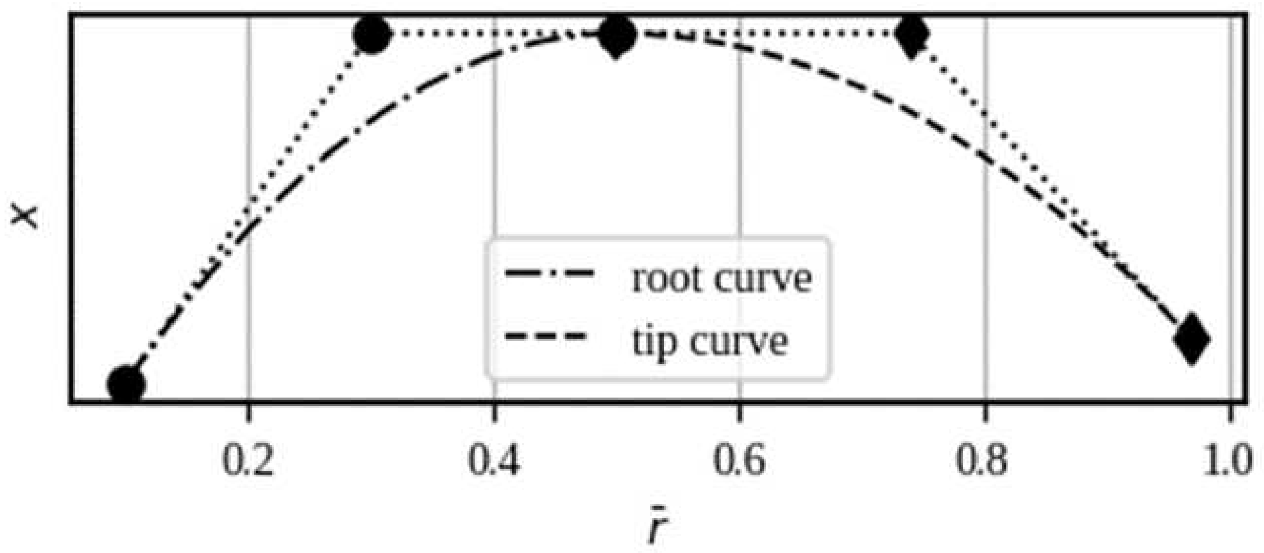
Figure 2.
Airfoil construction using cubic Bezier curves.
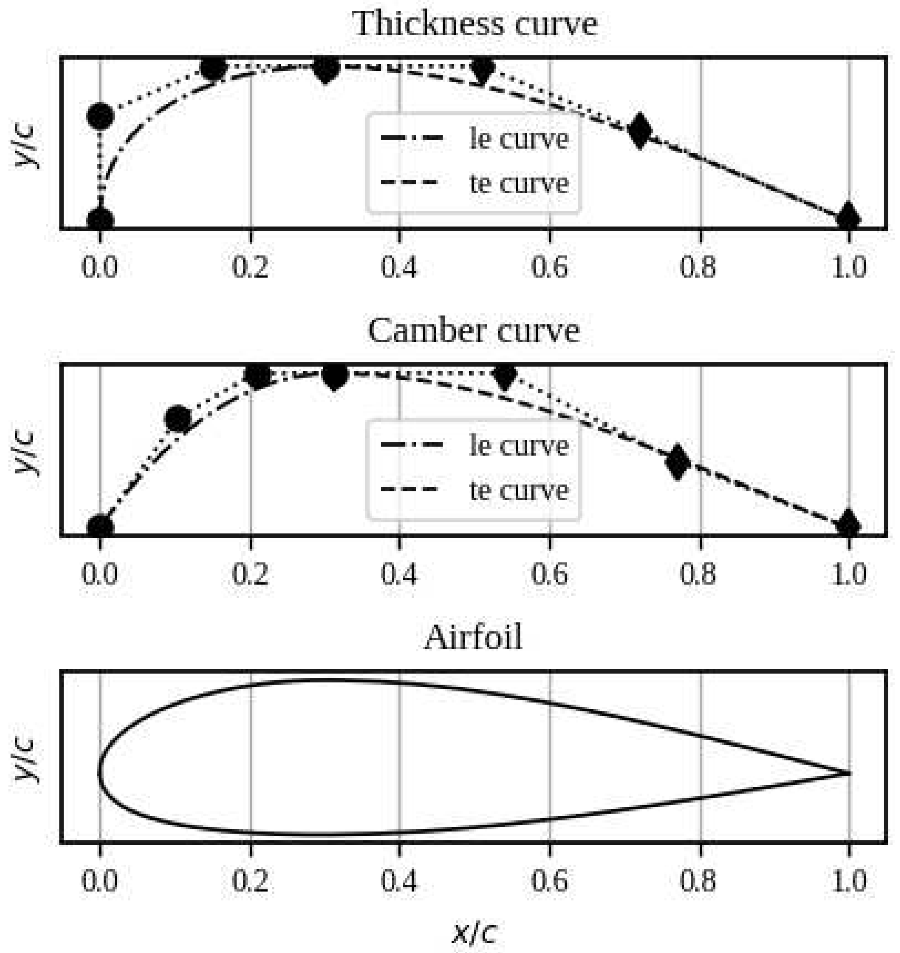
Figure 3.
Aerodynamic coefficients of the CLARK Y profile by different methods.
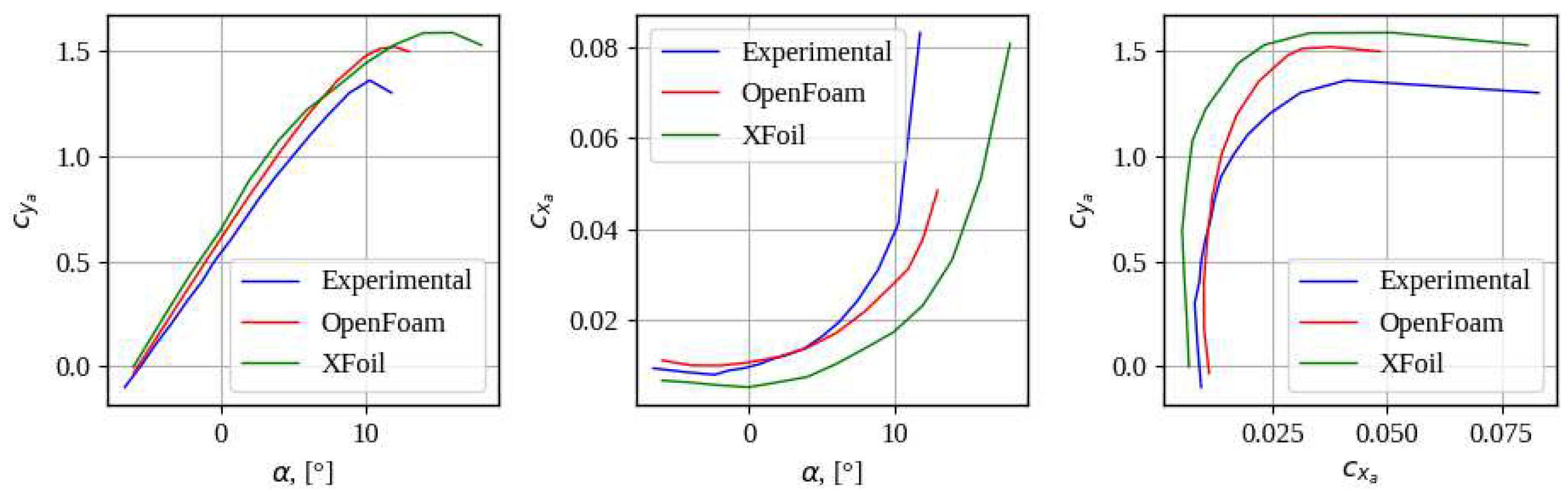
Figure 4.
Calculation and interpolation of aerodynamic characteristics of the profile by propeller span.
Figure 4.
Calculation and interpolation of aerodynamic characteristics of the profile by propeller span.
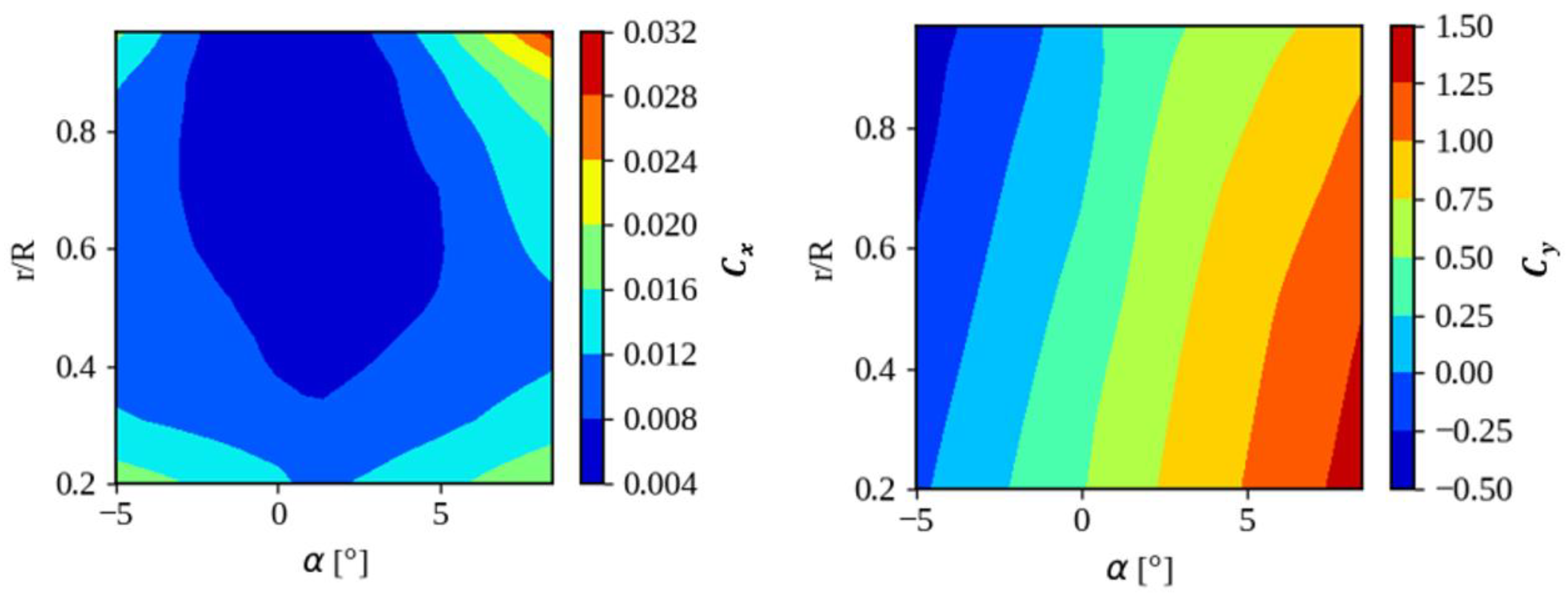
Figure 5.
Comparison by thrust coefficient (a) and power coefficient (b).
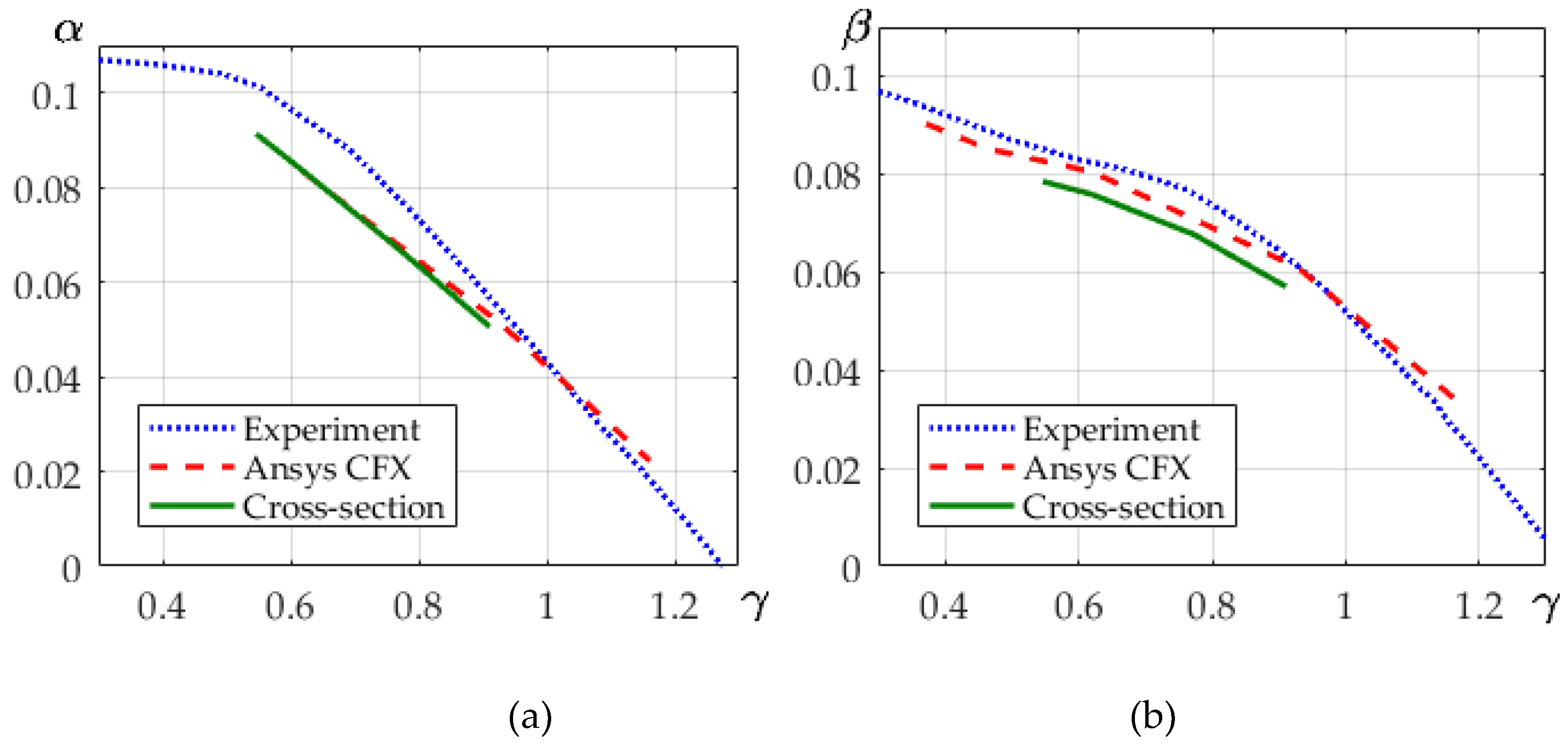
Figure 6.
Metrics of the optimization process.
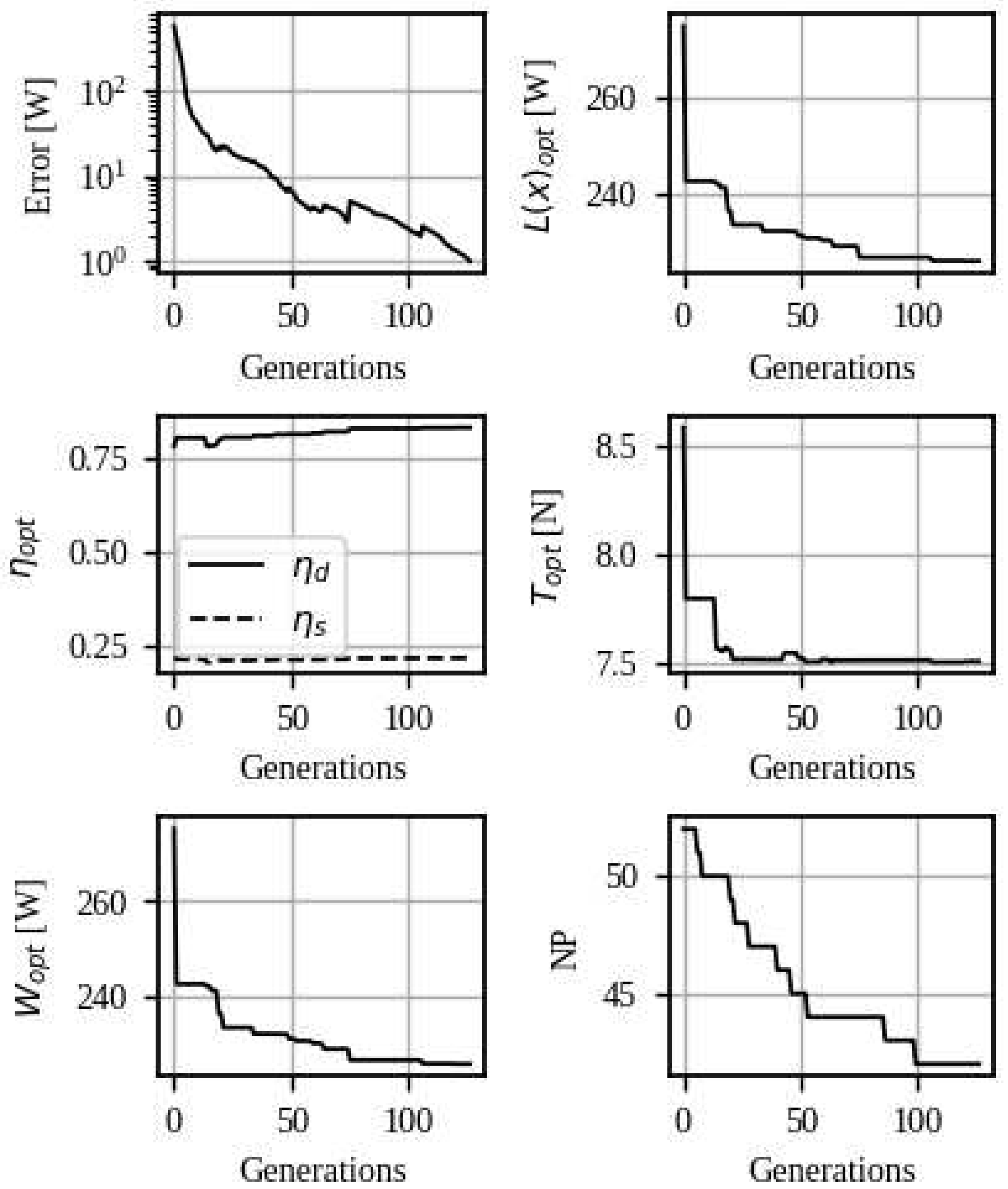
Figure 7.
Geometric characteristics of the optimal propeller.
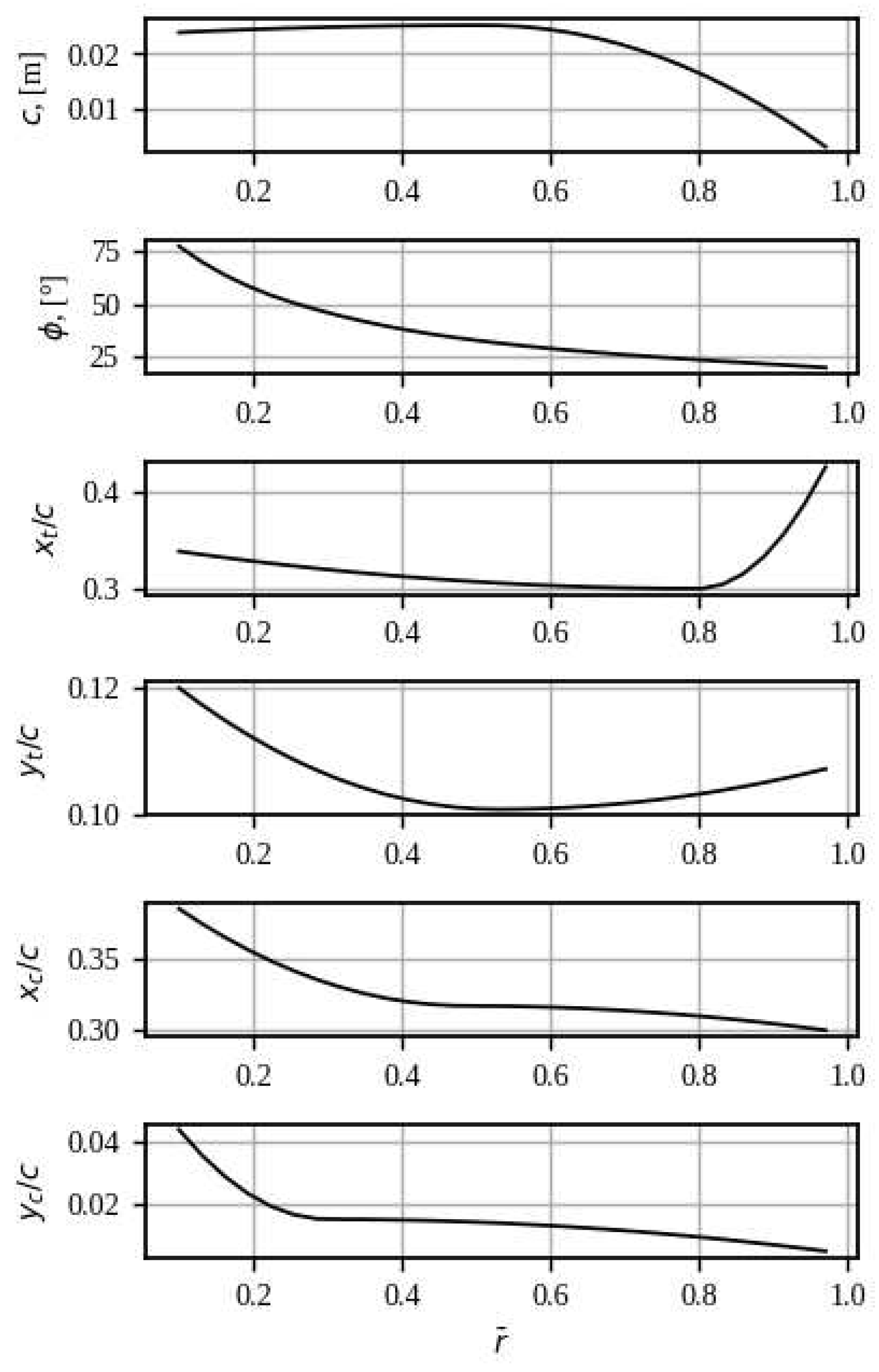
Figure 8.
The general view of the propeller and the shape of the airfoils in each section in of the propeller blade.
Figure 8.
The general view of the propeller and the shape of the airfoils in each section in of the propeller blade.
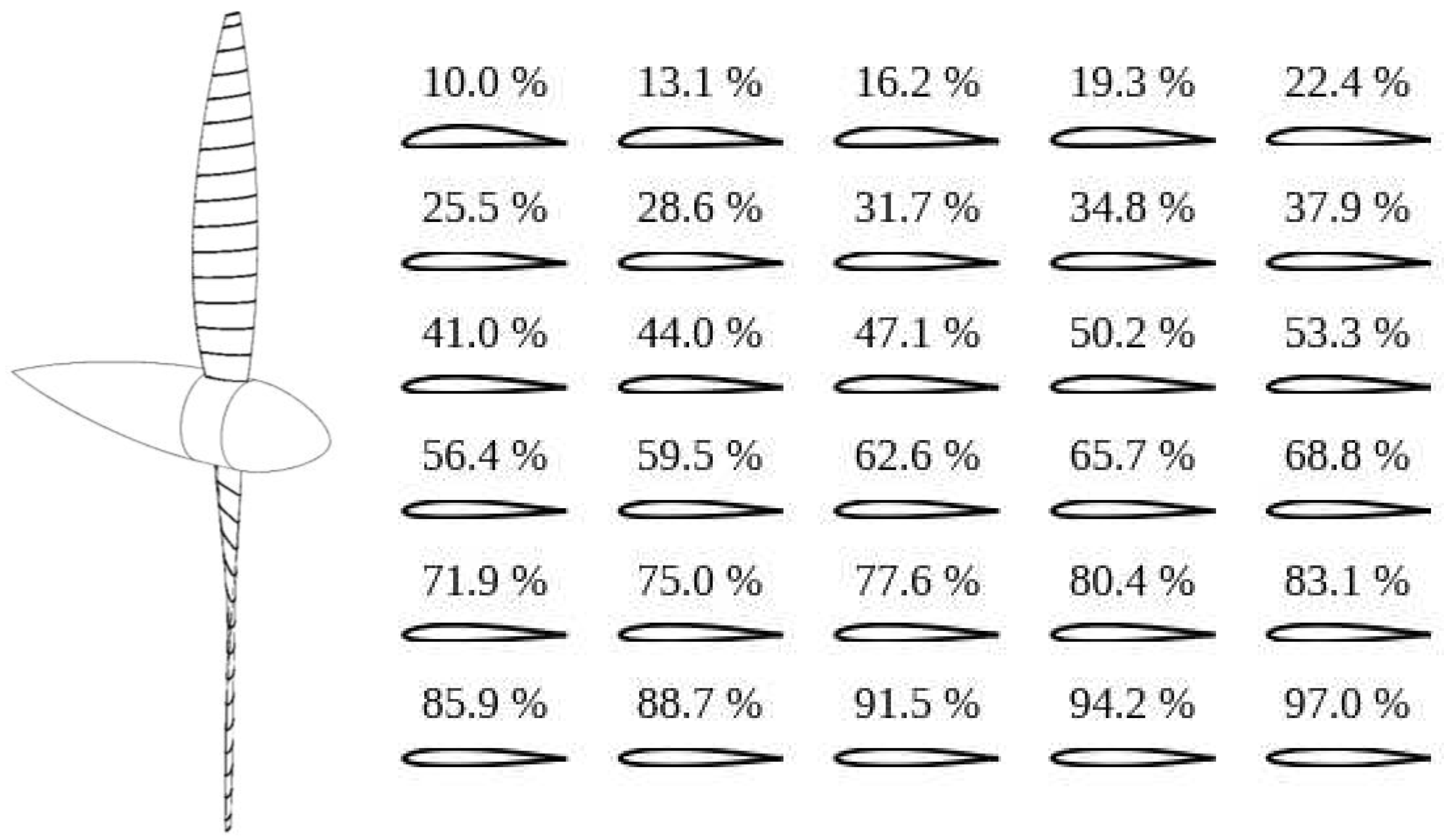

Table 1.
Intervals of the design variables.
| Variable | Interval | Variable | Interval |
|---|---|---|---|
| (c/d)r | [0.03, 0.10] | xtt | [0.30, 0.45] |
| (c/d)m | [0.03, 0.10] | r̅xtm | [0.30, 0.80] |
| (c/d)t | [0.01, 0.02] | ycr | [0.01, 0.05] |
| r̅cm | [0.35, 0.60] | ycm | [0.01, 0.05] |
| αr | [-7, 7] ° | yct | [0.005, 0.05] |
| αm | [-5, 7] ° | r̅ycm | [0.30, 0.80] |
| αt | [-5, 7] ° | xcr | [0.30, 0.40] |
| r̅αm | [0.25, 0.75] | xcm | [0.30, 0.45] |
| ytr | [0.12, 0.20] | xct | [0.30, 0.45] |
| ytm | [0.12, 0.16] | r̅xcm | [0.30, 0.80] |
| ytt | [0.10, 0.12] | nm | [5e3, 10e3] rev/min |
| r̅ytm | [0.30, 0.80] | B | [2, 4] |
| xtr | [0.30, 0.40] | d | [0.3, 0.3] m |
| xtm | [0.30, 0.45] |
Table 2.
Optimal vector.
| Variable | Value | Variable | Value |
|---|---|---|---|
| (c/d)r | 0.0798405 | xtt | 0.42644 |
| (c/d)m | 0.0842341 | r̅xtm | 0.8 |
| (c/d)t | 0.010028 | ycr | 0.0439051 |
| r̅cm | 0.513672 | ycm | 0.0152008 |
| αr | 7 ° | yct | 0.005 |
| αm | 4.71326 ° | r̅ycm | 0.3 |
| αt | 5.23632 ° | xcr | 0.385744 |
| r̅αm | 0.2543 | xcm | 0.317216 |
| ytr | 0.12 | xct | 0.3 |
| ytm | 0.1007486 | r̅xcm | 0.487034 |
| ytt | 0.1071704 | nm | 6896.51 rev/min |
| r̅ytm | 0.52874 | B | 2 |
| xtr | 0.338746 | d | 0.3 m |
| xtm | 0.3 |
Disclaimer/Publisher’s Note: The statements, opinions and data contained in all publications are solely those of the individual author(s) and contributor(s) and not of MDPI and/or the editor(s). MDPI and/or the editor(s) disclaim responsibility for any injury to people or property resulting from any ideas, methods, instructions or products referred to in the content. |
© 2023 by the authors. Licensee MDPI, Basel, Switzerland. This article is an open access article distributed under the terms and conditions of the Creative Commons Attribution (CC BY) license (http://creativecommons.org/licenses/by/4.0/).
Copyright: This open access article is published under a Creative Commons CC BY 4.0 license, which permit the free download, distribution, and reuse, provided that the author and preprint are cited in any reuse.


