Submitted:
08 November 2023
Posted:
09 November 2023
You are already at the latest version
Abstract
Gravitational data are the only ones able to provide otherwise hidden details of what happens below the surface. In this paper, several models are implemented to constrain them with the outer structure of Mars: firstly a Bouguer inversion to reduce gravitational residual, obtaining a crustal depth in the range 23.19-94.56 km. Successively, it was considered an Airy model providing for local buoyancy. Given that its configuration does not permit to evaluate properly the different flexural responses of the lithosphere, and that it overcompensates for the crust of the highest volcanic conformations, a flexural response function was used to filter this model. It uses the lithosphere elastic thickness T_e to scale especially the short wavelengths, correcting for local phenomena. Finally, an optimization was implemented to find the best-fitting values for T_e, using both an infinite plate and a thin shell approximation, and then obtain a global map for crustal density and thickness. Even if the Martian dichotomy is basically confirmed by all the models, along with the well-known anomalies localized at the major basin craters and volcanic Paterae, the Bouguer model supplies the best representation of the state-of-the-art knowledge about the outer layers of Mars and with further improvements can represent a future benchmark for the research on the Red Planet.
Keywords:
Mars
; Geophysics
; Bouguer
; Gravity Models
; Planetary Interiors
; Crustal Variations
1. Introduction
1.1. Purpose of this Study
The study of a planet’s interiors is crucial to understanding its history and evolution, the processes it underwent, and their consequences on the superficial ecosystem. In such a way, even a world that can appear desolate and mortifying as Mars can provide precious insights into planetary evolution that can help us improve our knowledge of the Earth.
Consequently, if the previous studies were focused on the building of Mars’s interior structure and its principal physical properties, and successively on the responsive behavior of the viscous layers when solicited by a mechanical load, this paper will analyze another discriminating factor that characterizes any body in the Universe: gravity.
Gravitational data are the only ones able to provide otherwise hidden details of what happens below the surface, helping to understand not only the spatial variations of parameters like density and thickness (as in the works of Beuthe et al. [1] and Goossens et al. [2]) but also possible dynamic processes on larger scales as mantle plumes (as suggested by the work of Broquet and Andrews-Hanna [3]).
In an attempt to join this thriving literature on the subject, this study will start from the topographical data obtained by MGS (Mars Global Surveyor) and from the gravitational data obtained by MRO (Mars Reconnaissance Orbiter) to then implement different models capable of matching their constraints. By doing so, it would be possible to better understand the main Martian features and, by studying the discrepancies between observations and models, as well as between each model, it would be possible to assess possible explanations for global anomalies.
1.2. Reference Models
The starting point for this research cannot be different from citing and introducing some reference models from the literature.
The first one is the work of Thiriet et al [4], focused on analyzing and comprehending the hemispherical dichotomy between the northern and southern regions of Mars. By means of Monte Carlo simulations, they investigated the evolution over geological eras of the lithosphere’s elastic thickness, trying to understand the reasons behind the differences between North and South.
Essentially, they first managed to solve the energy balance equation for the core, the mantle, and the stagnant lid (namely, the lithosphere). Considering that this aspect serves only to study the variations in crustal composition, they assumed a well-mixed mantle and core, as well as a constant mantle heat flux - that does not take into account the possible presence of mantle plumes.
Successively, they provide for the computation of the elastic lithosphere thickness. These calculations rely on two major components: a brittle deformation, as a consequence of the lithospheric pressure, and a ductile creep, dependent on the temperature profile, the strain rate, and the lithospheric rheological parameters. In particular, this last aspect forces them to differentiate the calculation between the crust and the mantle, as their rheologies and temperature profile are different. Consequently, the elastic lithosphere thickness is given by the following formula:
At the end of their work, they succeed to find optimal values - shown in Table 1 - that are able to explain the dichotomy only taking into account both a significantly smaller density and a higher enrichment in radioelements for the southern hemisphere.
Although their approach allows building a completely different model with respect to the ones that will be implemented here later, their results can actually be crucial in validating this study: coming from very different paths, similarities and differences can lead to a more effective understanding of the limits and advantages of both models.
The second model is, instead, represented by the work of Neumann et al. [5]. If in the first reference the analysis was tackled in a completely different way, in this one the starting point is actually the same: they retrieved topographic and gravitational data from MGS measurements in order to construct a Bouguer Map and then a global model for crustal densities and thicknesses.
Constructing a gravitational model for the Martian crust, they investigated the spherical harmonics signals from order 3 up to around order 72. In this way, they cut off the signal of the lowest degrees, corresponding to large-scale contributions such as mantle convection and the dual effect of the dynamic topography and the hydrostatic flattening of the mantle-core boundary, and at the same time, they avoided noises from the highest order, caused by limits in the sensibility of the instrumentation.
Successively, performing an inversion on the Bouguer anomaly, they iteratively changed the depth of the Moho discontinuity - firstly assumed at -45 km - to minimize the residuals and therefore construct a crustal thickness map, in a way that is almost identical to what will be done here later. In the end, their conclusion shows results - shown in Table 1 - that underline how the south of the planet is coherent with the observations only considering a crust less dense than the average: only in that way their thinnest region, the Isidis Planitia, keeps physical values of thickness.
Concluding their work, they also investigated the major impact features and volcanic spots in order to estimate visible consequences inherited by the crust and the mantle to the present day. Anyway, the details of this part will be discussed later in the paper when necessary to explain and compare some results.
Thus, without waiting further, in the following section it will be possible to get familiar with the study, precisely with the topography and the gravity of Mars.

Table 1.
Main parameters from the reference literature. Note that for the work of Thiriet et al [4], the lithosphere elastic thicknesses come from estimates under the polar ice caps that they assumed valid for the totality of the hemispheres.
Table 1.
Main parameters from the reference literature. Note that for the work of Thiriet et al [4], the lithosphere elastic thicknesses come from estimates under the polar ice caps that they assumed valid for the totality of the hemispheres.
| Variable | Thiriet et al. | Neumann et al. |
| d (km), (kg/) | (2018) | (2004) |
| 30-55 | 32 | |
| 40-96 | 58 | |
| ≥ 293 | 150 | |
| ≥ 193 | 150 | |
| 3100 | 3100 | |
| 2530-3100 | 2700 | |
| 3500 | 3500 |
2. Topography, Gravity and Bouguer Anomaly
As mentioned in Section 1, gravity and topography data come directly from MRO and MGS measurements, respectively. In detail, the data sheets were retrieved from the PDS Geosciences Node database [6,7]; they provide both an image outlining the geological features of the planet with an accuracy of four pixels per degree and its spherical harmonics coefficients up to degree 120.
Anyway, for the purpose of this study, the analysis of the spherical harmonics domain will be limited to the first 80 degrees or, when specified, to the first 50. This choice will simplify the analysis of the results, avoiding possible errors due to noises of the smallest wavelengths. Additionally, the topographical data will be compressed to 1 pixel per degree performing a mean; in this way, they can fit with the gravitational data and lighten the computations.
In Table 2, it is possible to see the main parameters used for the modeling of Mars, along with a schematic of the outer layers of the planet. In Figure 1a,b, instead, it is presented the topographic and gravitational maps. For the latter, the coefficient of the spherical harmonics was set equal to 0 to ignore the effect of the flattening due to centrifugal force.
In order to produce the Bouguer Anomaly Map from Figure 1c, the following approach was applied:
-
The Bouguer correction was computed using the formula:This step permits taking into account the contribution of the topography (thus, the attraction of each column of rocks) at each point of the map;
- The gravitational data were corrected turning off the coefficient and . If the latter was already ignored before, the former is now set to 0 to eliminate the contribution of the mean gravity over the planet and keep only regional signals.
- The Bouguer Anomaly can be now computed, essentially following the formula:
This map is essential to start understanding the crustal structure of a planet: considering that the model is assuming a constant density for the crust, and moreover lower than the mantle’s one, positive values for the anomaly should match with more mass under the surface and consequently a thinner crust. This is the case of depressions such as Hellas, Isidis, and Utopia Planitiae or Argyre Planitia (for accurate positioning over the Martian globe, see Appendix A), but also of Olympus Mons which is actually unusual. In fact, mountains or mass conglomerates are usually compensated by a thickening of the crust in the advantage of a thinning of the mantle - and, as visible for the Tharsis and the Elysium Regions, they present negative anomalies. The Olympus Mons, nevertheless, shows an unexpected behavior that can be explained by considering a denser surface composition due to infiltration of magmatic flows in crater basins below the patera [5,6].
However, these are only the first insights given by gravity measurements. In the following section, numerical modeling will provide an interpretation of these data and their influence on global crustal thickness variations and local anomalies.
Figure 1.
Topography, Gravitational data, and Bouguer Anomaly of Mars.
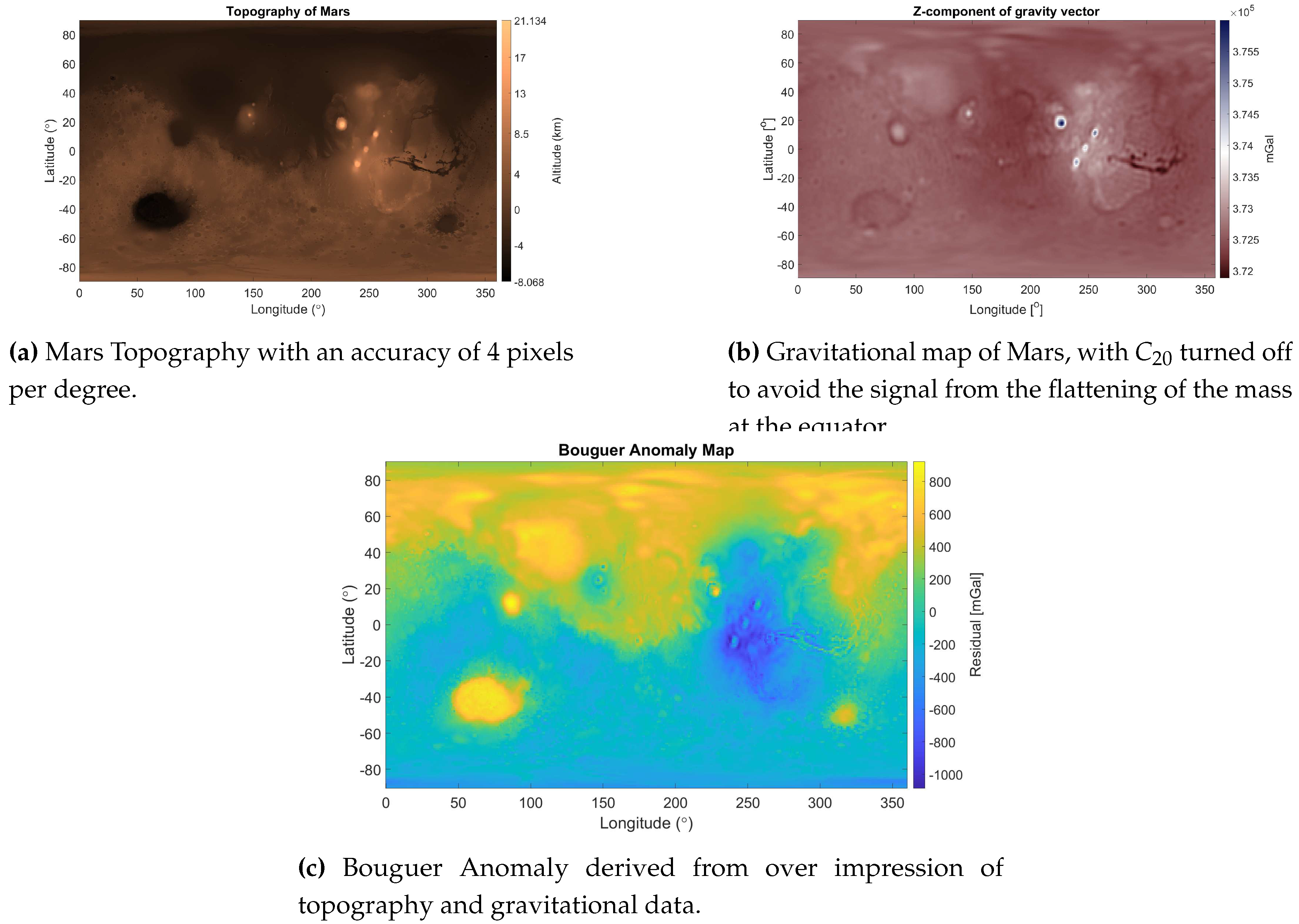
Table 2.
Main parameters of Mars and a schematic of the modelization of the outer layers of the planet. Note that refers to the distance at which the gravity is computed, that in this case is 0 which means on the surface of Mars. The boundaries of the layers - 3 in total - were chosen to avoid problems with the discretization: the layers were kept as close as possible to 25 km - that is the width the code uses to discretize the planet over its circumference - to avoid numerical errors.
| Constant | Value | Reference |
| GM | N/kg | [7] |
| 3389.5 km | [8] | |
| 0 km | (-) | |
| - 33 km | (-) | |
| - 65 km | [4] | |
| - 90 km | (-) | |
| 2850 kg/ | (-) | |
| 2850 kg/ | [9] | |
| 3500 kg/ | [4,5] |
3. Bouguer Inversion for Crustal Thickness
With the scope to map the crustal lateral variation in density, a discretization scheme, able to model the Martian crust, was chosen and iterated. As visible in Table 2, three layers were considered:
- A first one, enclosed between the topography and a depth of -33 km; considering that the lowest point of the topography is at -8 km, it was reasonable to place the boundary at a distance of 25 km.
- A second one, enclosed between -33 km and -65 km, the latter corresponding to the Moho discontinuity. This boundary was chosen accordingly with the results of Thiriet et al. [4], which found a mean crustal thickness in the range of 40-72 km around the globe, but moved more towards the southern values to take into account the greater surface area.
- A third one, between -65 km and -90 km, representing the transition between the crust and the lithosphere.
As cited before, assuming constant densities and thicknesses for the crust, the gravitational data cannot be fitted perfectly: the Bouguer Anomaly, in fact, shows the residuals of this approximation. The first approach is thus to keep a constant density for the crust - extended also to the geological features of the topography, for simplicity - and iteratively vary the Moho boundary at each point of the globe proportionally to the residuals. In this way, a positive residual moves the boundary up, and vice-versa for a negative one.
In the numerical setup, particular attention was paid to the proportionality factor. In fact, a too-high choice often results in inaccuracies of even 500 meters, while a too-low one slow-downs the computational time. Therefore, a factor of 80 was picked as a trade-off to reduce the mean of the residuals - that was the convergence target - of two orders of magnitude, for then passing to 300 and 500 for the other two orders of magnitude. During the iterations, the ratio of the standard deviations of modeled to real gravity data was also monitored to keep track of the consistency between the two models.
In addition, a specific section of the code avoids the possibility of overlapping between the Moho and the other boundaries: in the case this happens, the interested points are overwritten with the new values of depth, permitting the evaluation of those portions of the layers only once.
Finally, the convergence was performed on the basis of the first 50 degrees of spherical harmonics, ignoring also the first two. If this last choice is again driven by the necessity to avoid large-scale events, the degrees over 50 were neglected to take into account a safer margin from noise. In fact, Neumann et al. [5] implemented a dedicated filter to safely treat the highest degree, but this strategy was not applied here. As an effect, some regions of the map may appear more blurred.
The results, shown in Figure 2b, confirm two general and different behaviors for the two hemispheres: the northern crust is globally thinner, while the southern one is wider. This trend finds confirmations in the literature, and a proposed explanation recalls the possibility of a huge impact, occurred in the north, that forced an isostatic enlargement of the southern crust [4]. This event, in addition, would also explain possible differences in crustal composition between the hemisphere, considering super-isostatic events that may have brought mantle materials up to the southern surface.
Nevertheless, the most prominent geological conformations leave their own footprint on the map, creating marks that may be in contrast with the neighborhood. This happens for the main crater basins and Paterae, as well as for the ice caps at the poles, which follow the pattern mentioned in Section 2 but the trend is still anomalous for Olympus Mons, confirming the peculiarity of such feature.
In Figure 2a, it is possible to see the residuals at the end of the iterations. All of them are limited to a range of a few decimals of mGal - although starting from the thousands of the Bouguer anomaly - and don’t present the typical geological pattern. For a better comprehension of the implications that the assumptions bring to the model, a sensitivity analysis was performed and its results are shown in Figure 2c and in Table 3. It was decided to vary, alternatively, the density of the topography and of the layer below - that is the layer constrained by the Moho discontinuity - to understand their influence on the computation and on the structure. From the picture, it is noticeable that higher densities for the topography layer correspond to higher initial errors, and lower densities for the rest of the crust mean faster convergence. This is likely due to the fact that a denser topography requires globally more changes below to fit the gravitational data, increasing thus the initial error; moreover, a lighter crust compensates less for the weight above, speeding up the process of thickening or thinning under the more delicate spots.
Nonetheless, this explanation finds only partial confirmation in the results shown in the table. Indeed, if lower density contrasts between the crust and the mantle should imply higher deformations of the Moho discontinuity [5], as it happens for the second and the third case, in the last case the highest boundary is much closer to the surface than in the benchmark. The explanation for this relies on the fact that, for this setup, the thinnest crust is located below Olympus Mons, instead of the Hellas Planitia. Therefore, it is that singular point that is impossible to explain with such a low density for the topography. Another piece of evidence enforcing the presence of dense structures inside the Paterae of the Mons.
Figure 2.
Results from Bouguer Model for the global crustal thickness (a,b,c); Results from Airy Model for the global crustal thickness (d); Results from the flexural corrected Airy Model for the global crustal thickness (e).
Figure 2.
Results from Bouguer Model for the global crustal thickness (a,b,c); Results from Airy Model for the global crustal thickness (d); Results from the flexural corrected Airy Model for the global crustal thickness (e).
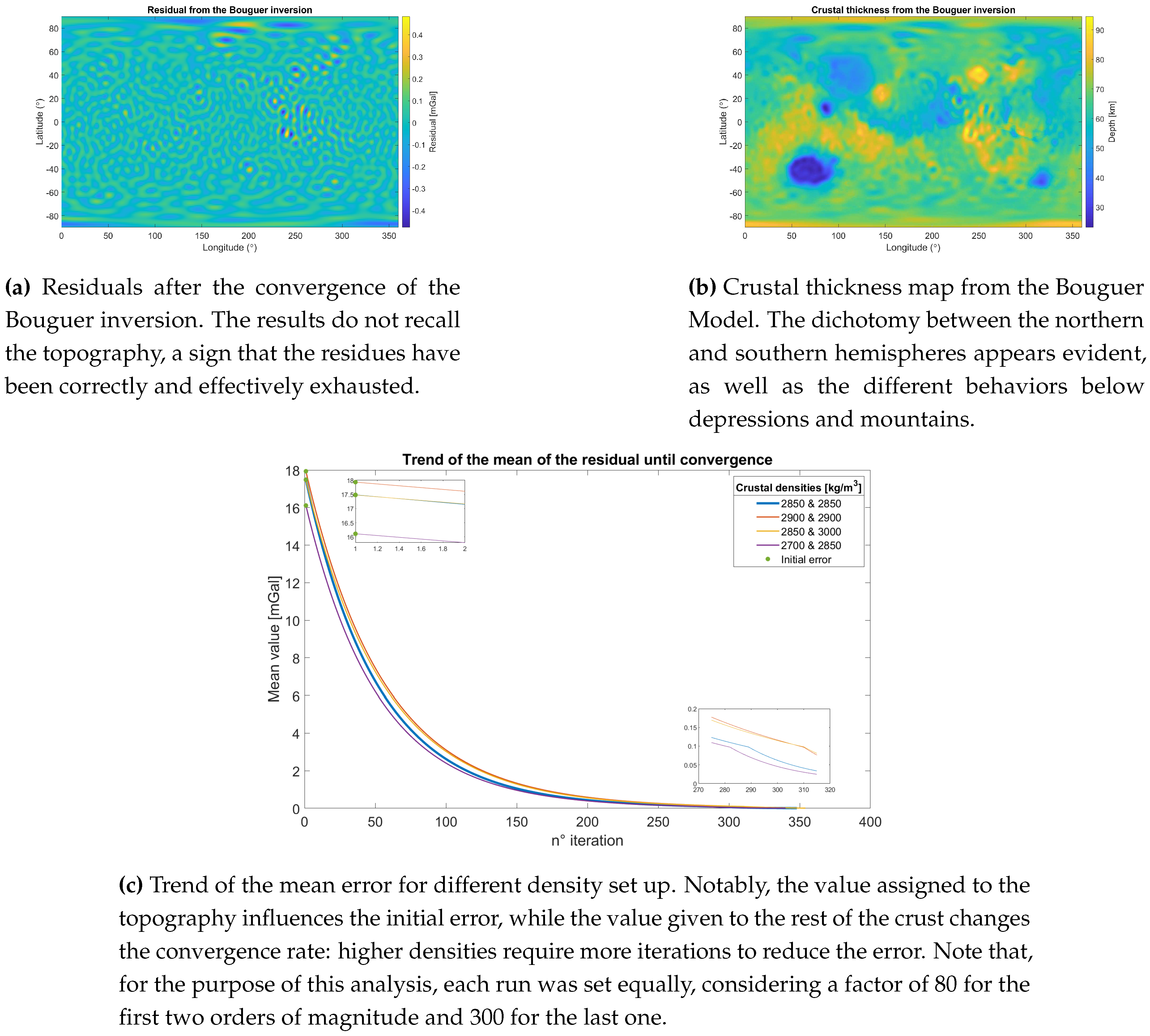
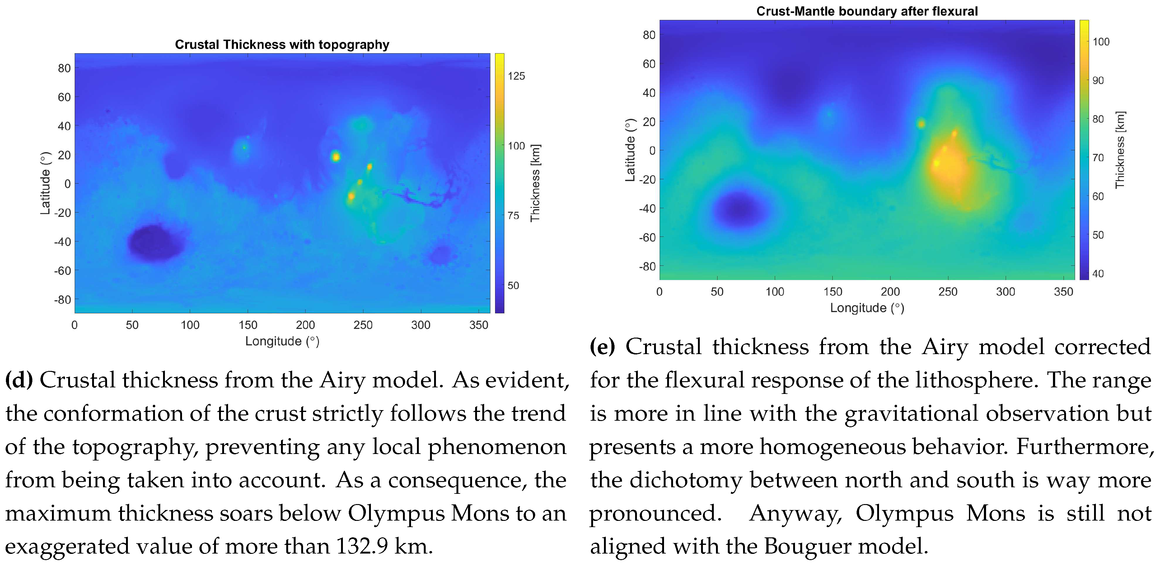
Table 3.
Different combinations applied for the sensitivity analysis of the Bouguer model, and respective highest and lowest points reached by the Moho discontinuity.
Table 3.
Different combinations applied for the sensitivity analysis of the Bouguer model, and respective highest and lowest points reached by the Moho discontinuity.
| Highest boundary | Lowest boundary | ||
| (kg/) | (kg/) | (km) | (km) |
| 2850 | 2850 | -21.83 | -89.74 |
| 2900 | 2900 | -20.62 | -96.84 |
| 2850 | 3000 | -19.97 | -93.72 |
| 2700 | 2850 | -18.82 | -87.62 |
4. Airy Model and Corrected Airy Model
For the next steps in this study, an Airy model will be constructed. It is very similar to the Bouguer model, in the sense that it keeps the density of the crust constant while varying its thickness. However, in contrast with the Bouguer approach that compensated for gravitational anomalies, the Airy model compensates for the local isostasy of each material column on the surface of the planet, more precisely discretizing with one column for each degree of latitude and longitude. Therefore, its response is pretty proportional to the pattern of the topography:
Where h is precisely the altitude of the topography, and the remaining proportional factor keeps track of the density variation between crust and mantle.
Nevertheless, this approach falls into oversimplifying the response of the crust, generating thicknesses that follow the geological features - as visible in Figure 2d - and do not take into account local phenomena. As a consequence, the range of thickness assumes strange values that are in conflict with other models and satellite measurements. In order to buffer at least partially this discrepancy a flexural correction is applied to the model.
This filter permits to evaluate also the effect of the deflection of the elastic lithosphere when loaded at the surface, and it is applied to the spherical harmonics coefficients calculated after the simplified Airy model. It depends on the regional isostasy of the lithosphere, thus on its rigidity D:
Where is the lithosphere elastic thickness, E is the elastic modulus, and is the Poisson’s ratio of the elastic lithosphere. The values used for them are reported in Table 4. The complete formula for the filter is instead:
Where n determines the order of spherical harmonics to which applies this flexural response function - valid for the approximation of infinite plate - and R is the radius of the planet.
Figure 2e is representative of the crustal thickness that derives from this filter, and compared with the results from the Airy model it is evident the introduced effect: the lateral variations are smoother, and the range is narrower than before. This is linkable to the fact that each material column is no longer treated on its own but as a combined effect on the landscape; furthermore, each order of spherical harmonics is tuned differently, permitting tuning signals from different wavelengths accordingly to their size.
Table 4.
Structural parameters used to compute the rigidity of Martian elastic lithosphere. Note that for the elastic thickness, the value is assumed as the arithmetic mean of the extreme found by Thiriet et al. [4]; additionally, Elastic modulus and Poisson’s Ratio come from the approach of Crane and Rich [10], but adapted to the case of this study.
| Parameter | Value | Reference |
| 205 km | [4] | |
| E | 110 GPa | [10] |
| 0.27 | [10] |
5. Degree Variance and best fitting
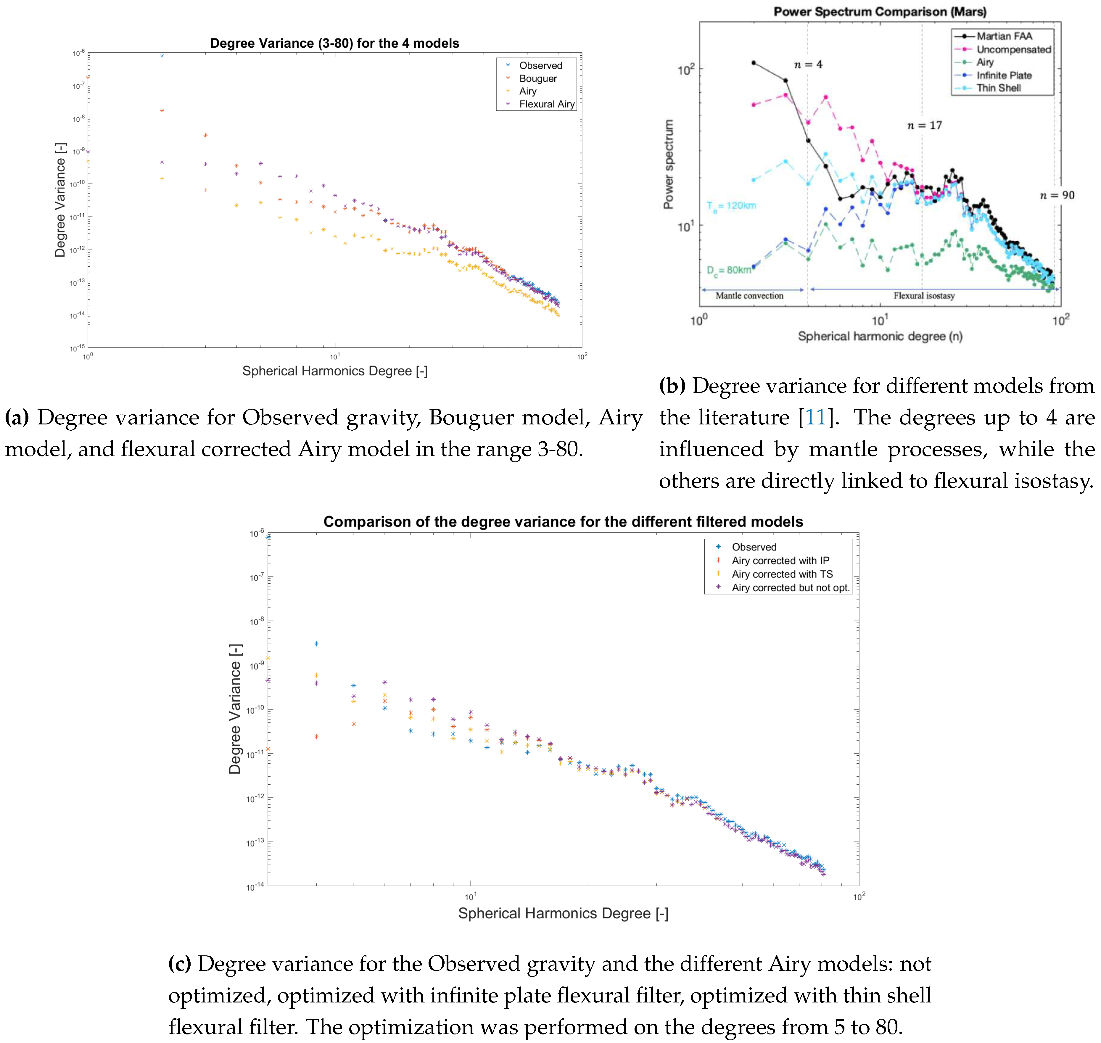
To assess the quality of the results obtained so far, a visualization of the degree variance of the spherical harmonics coefficients has been performed. This method permits keeping track of the dispersion of information in different frequency bands and for complex-valued spherical harmonics it can be computed as follow:
Where n refers to the degree of spherical harmonics, m to the order, C is the amplitude coefficient, and S is the complex phase coefficient.
In Figure 3a, it is possible to see four different trends, one for each of the data sets used so far: observed gravity, Bouguer model, Airy model, and Airy model corrected with a flexural response function. These degree variances give encouraging results:
- Except for degree 2, the Bouguer model almost overlaps perfectly with the observed data. This makes sense, considering that the Bouguer model was constructed on the observed data. The discrepancy, instead, can be attributed to mantle phenomena that were not considered in the simulation.
- The Airy model keeps always below the others. This is reasonable, considering that it provides for too-large thicknesses of the crust, therefore underestimating the gravitational response of the planet.
- The filtered Airy model, even if closer to its original for the lowest degree, degree by degree resembles the observed data set, meaning that is more true to reality.
To validate these results, Figure 3b was picked from literature [11]. It shows the Power Spectrum for the spherical harmonics degrees, which is the degree variance multiplied by a factor (GM/R. As visible, the general trend is pretty identical to the results of this study, with the only difference that the Airy model and the Infinite Plate - that corresponds to the filtered Airy model in Figure 3a - are more similar for the first degrees. This can be attributed to the small compensation thickness used in that model - only 80 km, with respect to the 205 km used in this work.
Another difference relies on the missing, in Figure 3a, of a curve for the Thin Shell flexural response. Actually, this model was implemented immediately after and is visible in Figure 3c, but it required the implementation of additional coding because is the result of an optimization.
In fact, the selected lithosphere elastic thickness of 205 km is an oversimplification. In order to improve it, a range of elastic thicknesses between 70 and 600 km was tested, with the objective to minimize the root sum squared of the difference between each degree variance of the Airy and the observed models. Furthermore, the aforementioned flexural response function , associated with an infinite plate, was compared with a more complex function, related to a thin shell. The latter should better take into account the response of such a small planet as Mars, where the global curvature cannot be easily neglected in favor of an infinite plate simplification.
The thin shell flexural response function is:
Two optimizations were performed, one using this filter and one using the infinite plate function, and the results are summarized in Table 5. The degree variance was corrected in the range between 5 and 80: the lower boundary was moved to 5 because, as visible from Figure 3b, the first four degrees are related to mantle convection, and fitting them would have required unrealistic values of lithosphere elastic thickness.
The degree variance in Figure 3c resembles almost perfectly the results from the literature, also because the best fitting from the thin shell model - 115.71 km - is very close to the reference. Additionally, the thin shell approximation adheres more to the observations with respect to the other, confirming the necessity to take into account the curvature of the planet. Nevertheless, the model still shows discrepancies: for the highest degree, where the optimization had no effect in moving the degree variance from the Airy model, and for the lowest degree, where the distance from the observations is still considerable. If the former would have required a tailor-made optimization, not influenced by the higher order of magnitude at the lowest degree, the latter implies the presence of deep mantle events such as plumes under the Elysium Planitia [3].
Table 5.
Results from the optimization with Infinite Plate and Thin Shell flexural response functions. As visible, Thin Shell requires less thickness and reduces better the discrepancies with the observed data.
Table 5.
Results from the optimization with Infinite Plate and Thin Shell flexural response functions. As visible, Thin Shell requires less thickness and reduces better the discrepancies with the observed data.
| Model | Best fitting | RSS |
| Thin Shell | 115.71 ± 1.5 km | |
| Infinite Plate | 177.76 ± 1.5 km |
Figure 3.
6. Inversion for Crustal Lateral Variations
The optimization performed in Section 5 has also influence on the depth of the Moho discontinuity in each portion of the planet, therefore modifying the crustal thickness map to match the observations. However, this passage does not definitively constrain the model: the maximum difference between the observed gravity and the gravity calculated from the best-fitting model - using the thin shell approximation - is near 840 mGal. Something is still missing: the assumption of constant density for the elastic lithosphere is too strict and has to be corrected.
A numerical setup was implemented to evaluate lateral variations of density: starting from the gravitational residual, an inversion provides for augmenting or diminishing the density depending on the sign of the discrepancy, respectively positive or negative. The process is quite similar to the convergence of Section 3, but here the proportionality factor is reduced to 15 to more definitely discretize the density variations, that in the code are already implemented in g/c.
Starting from the same mantle density used in the previous models - that is, 3500 kg/, keeping the same density for the crust (2850 kg/), but adjusting the lowest boundary to the best-fitting of 115 km, the final range for the lithosphere is shown in Figure 4a. Again, the singularity of Olympus Mons is quite evident: the density required to explain its gravitational anomaly, 4 kg/, may actually be not addressed in the lithosphere but on the surface. However, in this case also the other Tharsis Montes show the same behavior, indicating some sort of analogy among them in terms of composition and/or formation. Other elevations like Alba Patera and Elysium Mons, instead, deviate from this trend and align more with a traditional explanation. It may be linked to their position: they are more distant from the boundary between northern and southern hemisphere, therefore avoiding them to be affected by the geological processes happened near this trench [6].
Figure 4.
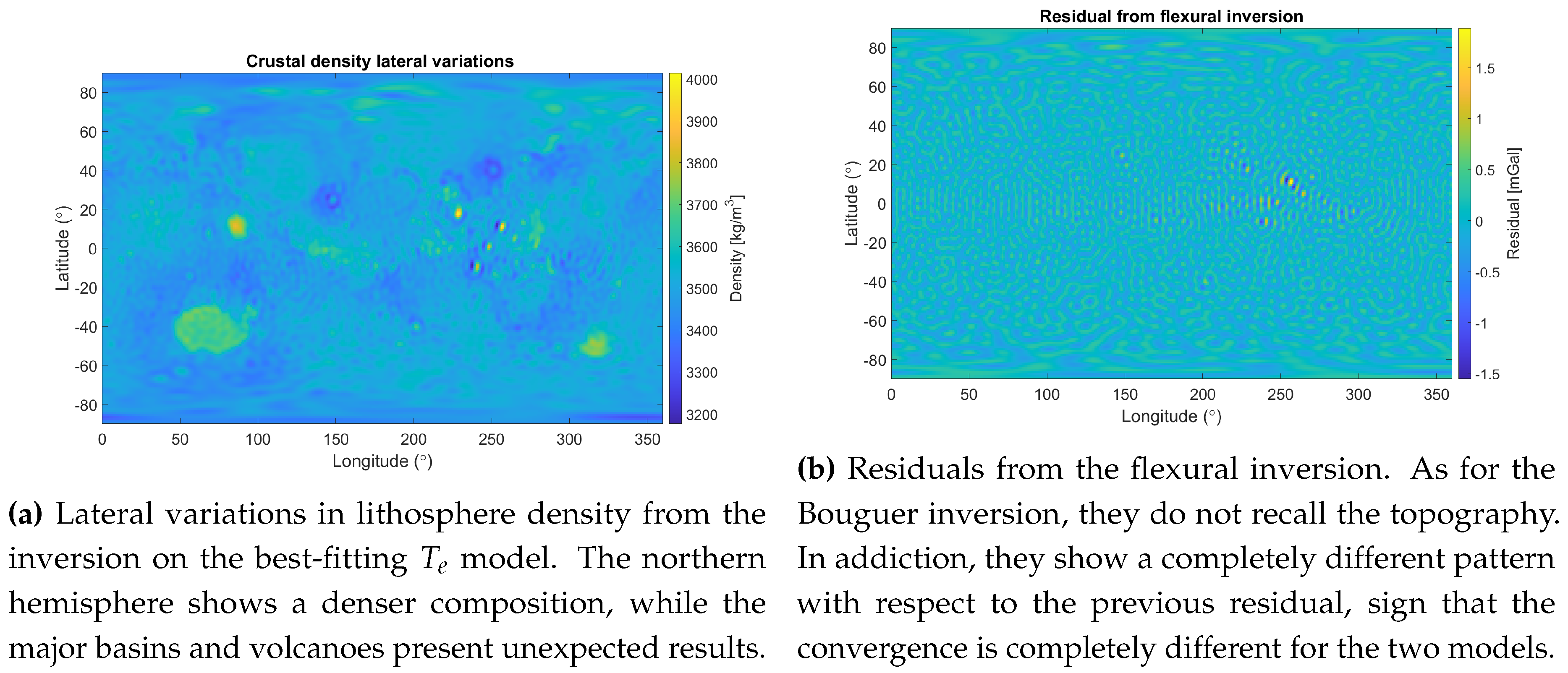
Another peculiarity is represented by the main crater basins, especially the Isidis Planitia. The required density of the mantle is exaggerated, especially considering the results obtained from the previous models in terms of thickness. A possible explanation for this comes from the work of Neumann et al. [5], where they fit the Isidis’ conformation assuming a superficial density of 3200 kg/ coming from magma infiltrations. Their model constrains the thickness with a maximum thickness of 45 km, thus avoiding the necessity of a super-isostatic mantle uplift. Anyway, they also suggest that a thicker crust would imply a too-dense mantle, and this seems the case in this model, where the crust extends for 65 km under Isidis - see Figure 5. And this theory is actually extendable to the other basins, more or less extensively.
The rest of the lithosphere repeats, even if less evidently, the global dichotomy of the surface.
Figure 5.
Crustal thickness from the optimized flexural model. The results for the main basins, Tharsis Montes, and Olympus Mons are slightly off with respect to the Bouguer model. The global dichotomy is instead evident.
Figure 5.
Crustal thickness from the optimized flexural model. The results for the main basins, Tharsis Montes, and Olympus Mons are slightly off with respect to the Bouguer model. The global dichotomy is instead evident.

7. Discussion and Conclusions
In an attempt to understand the information encoded in the outer layers of the Martian planet, this study went through different approaches and models, for which the results are summarized in Table 6. Starting from satellite data, a Bouguer map was constructed reducing the residuals between observed and modeled gravity. Successively, different isostatic models were implemented: an Airy model, then corrected by a flexural response function, then optimized with the thin shell approximation.
Table 6.
Major results from the models developed in this study, along with uncertanties. Note that, when these uncertanties do not depend on numerical modeling, conservative values - one order of magnitude greater - were considered on the measurements.
Table 6.
Major results from the models developed in this study, along with uncertanties. Note that, when these uncertanties do not depend on numerical modeling, conservative values - one order of magnitude greater - were considered on the measurements.
| Model | Parameter | Value |
| Bouguer | Max crust thickness | 94.56 ± 0.5 km |
| Min crust thickness | 23.19 ± 0.5 km | |
| Airy | Max crust thickness | 132.9 ± km |
| Min crust thickness | 32.7 ± km | |
| Flexural Airy | Max crust thickness | 105.5 ± km |
| Min crust thickness | 38.09 ± km | |
| Flexural Opt. | Max crust thickness | 74.8 ± km |
| Min crust thickness | 46.71 ± km | |
| Max litho. density | 4014 ± 0.5 kg/ | |
| Min litho. density | 3176 ± 0.5 kg/ |
The results that seem to better adhere to the literature are those coming from the Bouguer inversion. In fact, the minimum crustal thickness matches the requirement set by Neumann et al [5], which implies a thickness in excess of 6 km under the Isidis Planitia - and minimizes the distance from their result - 14 km. Even the maximum thickness is similar to their outcomes. However, the model presents many limitations - constant density for the topography and the crust, a limited amount of spherical harmonics degree - that need to be improved in further developments.
Moving on to the Airy model, it seems to overcompensate, with a too-thick crust, the presence of the main volcanic structures. Here the limitation, along with the aforementioned assumptions, comes from a constant lithosphere elastic thickness all over the globe. As shown by Thiriet et al. [4], in fact, this parameter can assume very different values in the two hemispheres, and local variations are more than probable considering their direct correlation with geological events over the evolution of Mars.
The same limits apply to the model filtered with the flexural response function, both in the non-optimized and in the optimized case. Further studies would require the compelling necessity to vary the density on the surface, to avoid wrong predictions for the lithosphere, in terms of both thickness and density.
Concluding, this study revealed once again that even a "dead" planet as Mars looks like today can actually hide an eventful and turbulent past. Whether justifying the gravitational anomalies of craters and volcanoes with a plume in the mantle or with a super-impactor, geological events have deeply marked the history of this planet, and only with future studies and missions, it will be possible to find out more about its past.
Acknowledgement
This paper was produced during the course "Physics of Planetary Interiors" within the Master’s Degree program in Space Engineering. The source code for all the results in this paper can be found in my GitHub directory: https://github.com/vinz2000/Assignment3.
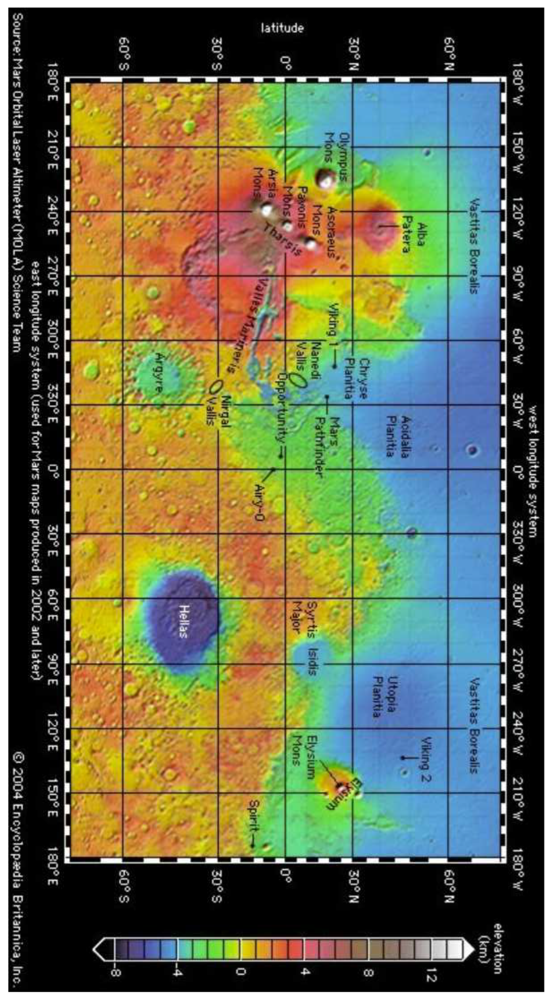
Appendix A. Geology of Mars
Figure A1.
Geology of Mars, with the main nomenclature. Retrieved by Britannica [14].
References
- Beuthe, M.; Le Maistre, S.; Rosenblatt, P.; Pätzold, M.; Dehant, V. Density and lithospheric thickness of the tharsis province from Mex Mars and Mro Gravity Data. Journal of Geophysical Research: Planets 2012, 117. [Google Scholar] [CrossRef]
- Goossens, S.; Sabaka, T.J.; Genova, A.; Mazarico, E.; Nicholas, J.B.; Neumann, G.A. Evidence for a low bulk crustal density for Mars from gravity and Topography. Geophysical Research Letters 2017, 44, 7686–7694. [Google Scholar] [CrossRef] [PubMed]
- Broquet, A.; Andrews-Hanna, J.C. Geophysical evidence for an active mantle plume underneath Elysium Planitia on Mars. Nature Astronomy 2022. [Google Scholar] [CrossRef]
- Thiriet, M.; Michaut, C.; Breuer, D.; Plesa, A.C. Hemispheric dichotomy in lithosphere thickness on Mars caused by differences in crustal structure and composition. Journal of Geophysical Research: Planets 2018, 123, 823–848. [Google Scholar] [CrossRef]
- Neumann, G.A. Crustal structure of Mars from gravity and Topography. Journal of Geophysical Research 2004, 109. [Google Scholar] [CrossRef]
- McGovern, P. INTERPRETATIONS OF GRAVITY ANOMALIES AT OLYMPUS MONS, MARS: INTRUSIONS, IMPACT BASINS, AND TROUGHS 2002.
- Konopliv, A.S.; Park, R.S.; Folkner, W.M. An improved JPL Mars Gravity Field and orientation from Mars Orbiter and lander tracking data. Icarus 2016, 274, 253–260. [Google Scholar] [CrossRef]
- (Chair), P.K.; Abalakin, V.K.; Bursa, M.; Davies, M.E.; Bergh, C.d.; Lieske, J.H.; Oberst, J.; Simon, J.L.; Standish, E.M.; Stooke, P.; et al. Celestial Mechanics and Dynamical Astronomy 2002, 82, 83–111. [CrossRef]
- Khan, A.; Ceylan, S.; van Driel, M.; Giardini, D.; Lognonné, P.; Samuel, H.; Schmerr, N.C.; Stähler, S.C.; Duran, A.C.; Huang, Q.; et al. . Upper Mantle Structure of Mars from Insight Seismic Data. Science 2021, 373, 434–438. [Google Scholar] [CrossRef] [PubMed]
- Crane, K.; Rich, J. Lithospheric strength and elastic properties for Mars from Insight Geophysical Data. Icarus 2023, 400. [Google Scholar] [CrossRef]
- Root, B. Physics of Planetary Interiors, 2023. Lecture slides.
Disclaimer/Publisher’s Note: The statements, opinions and data contained in all publications are solely those of the individual author(s) and contributor(s) and not of MDPI and/or the editor(s). MDPI and/or the editor(s) disclaim responsibility for any injury to people or property resulting from any ideas, methods, instructions or products referred to in the content. |
© 2023 by the authors. Licensee MDPI, Basel, Switzerland. This article is an open access article distributed under the terms and conditions of the Creative Commons Attribution (CC BY) license (http://creativecommons.org/licenses/by/4.0/).
Copyright: This open access article is published under a Creative Commons CC BY 4.0 license, which permit the free download, distribution, and reuse, provided that the author and preprint are cited in any reuse.


