Submitted:
30 October 2023
Posted:
03 November 2023
You are already at the latest version
Abstract
Single Image Super Resolution (SSIR) is a problem in computer vision where the goal is 1 to create high-resolution images from low-resolution ones. It has important applications in fields 2 such as medical imaging and security surveillance. While traditional methods such as interpolation 3 and reconstruction-based models have been used in the past, deep learning techniques have recently 4 gained attention due to their superior performance and computational efficiency. This article proposes 5 an Autoencoder based Deep Learning Model for SSIR, in particular, a light model that uses fewer 6 parameters without compromising performance. The down-sampling part of the Autoencoder 7 mainly uses 3 by 3 convolution and has no subsampling layers. The up-sampling part uses transpose 8 convolution and residual connections from the down sampling part. The model is trained using a 9 subset of the VILRC ImageNet database. The model is evaluated using quantitative metrics PSNR, 10 SSIM as well as qualitative measures such as perceptual quality. PSNR and SSIM figures as high as 11 76.06 and 0.93 are reported.
Keywords:
Single image super-resolution
; deep learning
; autoencoders
; convolutional neural net- 13 works
; convolution
; transpose convolution
; skipped connections
1. Introduction
In many applications in computer vision, such as security and surveillance imaging and medical imaging, there is a need to obtain a high-resolution image from the low resolution image captured at the site or in the lab. The problem of generating a high-resolution image given a low-resolution image is commonly referred to as Single Image Super Resolution (SISR). The fact that given a collection of low resolution pixels, there are more than one solution for the corresponding high resolution pixels make this problem difficult. A usual solution is to constrain the solution space using prior information about the scenery.
Common techniques for SISR can be mainly divided into three categories: interpolation-based methods, reconstruction-based methods, and learning-based methods. Interpolation based methods such as bi-cubic interpolation [1] and Lanczos re-sampling [2] are fast and straightforward but suffer from accuracy shortcomings. Reconstruction-based models [3,4,5,6], typically incorporate complex prior knowledge to constrain the set of feasible solutions, resulting in high-quality results with sharp and detailed outputs. Despite these advantages, many reconstruction-based techniques suffer from diminishing performance as the scaling factor increases, and are often computationally demanding.
Learning-based methods, also knows as example-based methods have gained popularity in recent years. These methods utilize machine learning algorithms to recover the relationship between the Low Resolution input and its corresponding high resolution counterpart. Learning-based methods have shown greater performance and lower computation time compared to all other methods. Very recently, deep convolutional neural networks have emerged as a powerful tool for solving the SISR problem.
A Convolutional Neural Network (CNN) is a type of machine learning algorithm that can automatically learn complex features in input image data [7]. This makes CNN a very powerful tool in various image processing tasks. Autoencoders were originally developed to learn a compressed, low dimensional, representation of the data in a large vector [8]. Autoencoders found a new application when scientists realized that the compressed representations could be used to generate a new variation of the original large vector. Eventually, deep Autoencoders that took in images, and used a CNN followed by a type of ‘reverse’ CNN were developed to create a new variation of the input image.
Several deep learning-based methods that have been proposed for the SISR problem use different variations on the Autoencoder architecture mentioned above. These methods have achieved state-of-the-art results in terms of both quantitative metrics and visual quality. However, there are still some challenges that need to be addressed, such as the trade-off between computation time and quality, the extent of generalization of a particular model across different domains and scales, and the need for more realistic evaluation metrics. Despite these challenges, the use of deep networks for SISR continues to be an active area of research, with new methods and architectures being proposed regularly.
In this article, we propose a novel approach for Single Image Super Resolution using Deep Convolutional Residual Neural Networks. Our model will be based on an Autoencoder structure which has Convolutional Neural Network (CNN) at the first half followed by a ‘reverse’ CNN on the second half mentioned above. The ‘reverse’ CNN part will perform upsampling using transpose convolution, and use skipped connections from the CNN part to enrich the collection of featuremaps on the second half. The article will examine the different metrics and loss functions used to achieve optimal performance. The focus is to design a light model that uses fewer parameters without a significant reduction in performance. The proposed approach will be evaluated using both quantitative and qualitative measures to compare the results of each model, including peak signal-to-noise ratio (PSNR), structural similarity (SSIM), and perceptual quality. Overall, our approach aims to provide a comprehensive and in-depth evaluation of deep learning models for super resolution and explore the design space for a more efficient and lightweight model.
The next section will present a brief overview of related works. Section 3 will outline the evolution of Autoencoders and the place of of the model used in this article. The problem statement, a description of the model, and the dataset used will be given in Section 4. The results will be discussed in Section 6, followed by conclusions in Section 7.
2. Related Work
This section presents a brief review of the work in image super resolution that used deep learning techniques.
Dong et al. [9] proposed a Super Resolution Convolutional Neural Network (SRCNN) that consisted three major components; patch extraction, non-linear mapping, and reconstruction . In the patch extraction layers, convolution filters extracted the image features without any subsampling (Figure 1). The non-linear mapping was performed by an artificial neural network. The reconstruction layer used bi-cubic interpolation to up-sample the low-resolution image. The model was trained using the Mean Squared Error (MSE) loss function and the results were evaluated using SSIM and MSSIM. It was reported that increasing the number of layers did not result in better performance. The article reported that the architecture is sensitive to learning rate and parameter initialization, and the depth of the network made it very difficult to set appropriate learning rates that guarantee convergence. The architecture reportedly achieved a PSNR of 32.52.
A model that uses a special, pre-trained, loss network instead of the pixel by pixel losses was developed by Johnson et al. [10]. The loss network used perceptual losses that depend on high-level features which produced visually appealing results. The model consisted of two main components; an image transformation network and a loss network (Figure 2). The transformation network used several residual blocks followed by convolutional layers. The results achieved were very visually pleasing. However, quantifying these results seemed to be a problem. In defence of [10], it should be noted that as reported in [11,12], PSNR and SSIM rely on per-pixel differences and correlate poorly with human assessment of visual quality, which is what this model is supposed to achieve.
Motivated by the small receptive field and the very slow training needed in the SRCNN [9], a Very Deep Super Resolution (VDSR) model was proposed in [13] that makes use of 20 convolutional layers. This very deep CNN network used gradient clipping techniques to handle exploding gradient problems. Moreover, the model was designed to learn the difference between the target Hi-Res image and the input Lo-Res image rather than learning the Hi-Res image directly. This resulted in significantly reduced the training time.
The introduction of ResNet by He et al. [14] opened the door for more advancement in Super Resolution. The core idea of ResNet is to enable a CNN network to be very deep without suffering from the vanishing gradient problem. ResNet layers were reformulated to learn residual functions with reference to the layer inputs, instead of un-referenced functions. These residual networks were easier to optimize and gained higher accuracy with increased network depth. A ResNet block constituted of one or more convolutional layer followed by a Batch Normalization and a ReLU activation.
The Super Resolution Residual Network (SRResNet) architecture was proposed by Ledic et al. [15]. Removing the Batch Normalization (BN) modules in the SRResNet architecture as proposed by Lim et al. [16] achieved better results. The model contained convolutional layers followed by residual blocks. The last part constituted of upsampling and convolution layers.
To make better use of the hierarchical features extracted from Low-Resolution images, Zhang et al. [17] proposed a Residual Dense Network (RDN) for Image Super Resolution that is also based on ResNet architecture (Figure 4 and Figure 5). This network modifies the residual blocks by connecting each layer to all subsequent layers in the block.
Since low resolution inputs and features contain low frequency information that are equally treated across channels, Zhang et al. [18] presented a model that selectively emphasizes informative channels in each feature map (Figure 6. This Image Super-Resolution Using Very Deep Residual Channel Attention Network (RCAN) is also based on ResNet architecture.
MSE loss function has its limitations when used in Super Resolution as it encourages average-like solutions that are not visually pleasing. Motivated by this, Ledig et al. [19] proposed a model for image Super Resolution using Generative Adversarial Network (SRGAN), the authors suggested a perceptual loss function which consists of an adversarial loss and a content loss. The adversarial loss pushes the solution to the natural image manifold by using a discriminator network that is trained to differentiate between the super-resolved images and the original photo-realistic images. The content loss is motivated by perceptual similarity instead of pixel-wise similarity. The generator network structure mainly consists of residual blocks each of which starts with two convolutional layers followed by batch normalization layers and ReLU as the activation function. One of the metrics used by the authors to evaluate the model is the Mean Opinion Score (MOS), 26 human raters rated the Hi-Res output images of this model compared to other SISR methods, the authors showed that the SRGAN model achieved the highest score compared to other models.
Yang et al. [20] reviewed deep learning methods used for Single Image Super Resolution (SISR) and summarized the trends and challenges ahead for Deep Learning (DL) algorithms in tackling the SISR problem. Firstly, the authors argued that lighter deep architectures for efficient SISR are needed. Even though very high accuracy for Hi-Res images from Lo-Res images was achieved, it is very difficult and impractical to deploy these models to real world scenarios, due to massive number of parameters and computational needs. They suggested that lighter models should be designed either from scratch or from slimming down current architectures without large compromise on performance. Moreover, the authors believed that more work should be done to bridge the gap in our understanding of deep models for SISR. The success of deep learning is said to be attributed to learning powerful representations. However, to date, these representations are not fully understood, and the deep architectures are treated as a black box. For DL-based SISR, the deep architectures are often viewed as a universal approximation, and the learned representations are often omitted for simplicity. This behavior is not beneficial for further exploration, and the authors argued that more work should be done on why and how these models work. That is, more theoretical explorations are needed. Lastly, the paper addressed the issue of not having rational unified assessment criteria for SISR. Most of the DL methods use the MSE as the loss function despite the fact that it has been shown as a poor criterion for SISR. Clear definitions for assessment criteria for SISR will help designing better optimization objectives and will make the comparison between models more rational.
3. Autoencorders
The deep learning model used in this article belong to a class of networks called Autoencoders. Autoencoders were originally developed for the purpose of dimensionality reduction [8]. They were used to learn a compressed representation of vector data. The simplest Autoencorders are Artificial Neural Networks with an hour-glass structure. These Autoencoders were trained with the input vectors as the targets. An Autoencoder that takes in a vector of size 1000 and reduces the dimension to 100 is shown in Figure 7. After training, the outputs from the bottle-neck layer in the middle produced a lower dimensional representation of the input vector.
Later on, researchers surmised that the compressed data could be used to construct a different version of the original input. In most of these applications, the inputs were often images rather than vectors (Figure 8). The input images were flattened and fed to the hour-glass ANN. A well known application of this is found in Image-de-noising networks.
Eventually Autoencoders dealing with images evolved to include the components from Convolutional Neural Networks (CNN) [7]. They used a U-shaped architecture, where the left side had a CNN and the right side had a ‘reverse’ CNN. A typical CNN has convolutional filters (Figure 9), featuremap layers, activations, and subsampled maps (Figure 10) followed by an Artificial Neural Network (ANN) that preforms the classification (Figure 11).
A convolutional filter moves around the image, takes dot products with the image at each location and places them on a featuremap. The convolution operation is illustrated in Figure 9. Maxpooling is a subsampling operation where a region in a featuremap is replaced by a single representative pixel. Maxpooling is explained in Figure 10. A simple CNN that uses two layers of convolution and maxpooling to extract features, and then uses an ANN to perform image classification is shown in Figure 11.
A typical Autoencoder structure is shown in Figure 12. It is important to note that the CNN on the left side of an Autoencoder does not end in an ANN. Rather, the CNN in an Autoencoder ends in a small featuremap. The right side of the Autoencoder starts with this small featuremap and uses transpose convolution and skipped connections from the left side to gradually build up the required output image.
The most important operation on the right side of an Autoencoder is the upsampling done by the Transposed convolution. The following example explains this operation. In Figure 13, a 3 by 3 transpose convolution filter operates on a featuremap of shape 4 by 4 pixel by pixel with stride 2 to produce an upsampled map. The filter kernels are multiplied by the pixel value in the top left corner of the feature map to generate a 4 by 4 submatrix. Now the filter moves to the right by one pixel and repeats the computation. The resulting submatrix is placed in the upsampled map after moving two pixels to the right. The calculations are shown step by step below:
Skipped connections in Autoencoders refers to the fact that some featuremaps from the CNN on the left side are copied and added to the collection of upsampled maps on the ’reverse’ CNN on the right side.
4. Problem Statement and the Model
The goal is to produce a deep neural network model that is capable of learning Hi-Res image given the corresponding Low-Res image. In particular, the purpose is to develop a lightweight model with a minimum number of parameters, in order to address the computational and resource constraints associated with the existing models. The architecture used in CNN part of the Autoencoder used in this article is borrowed from the state-of-the-art CNN called ResNet.
The Dataset to be used is a subset from the widely adopted imageNet database since this dataset was adopted by most of the models mentioned earlier and represent a benchmark for performance comparison.
5. Proposed Method
5.1. Proposed Network
The Low-Res input image, was first reshaped the to the size of 256x256x3. Let us denote the reshaped input image as . The aim is to recover a Hi-Res image from , and that for to be as similar as possible to the ground truth Hi-Res image .
The Autoencoder model used consists of 5 convolutional layers that down-sample the input image from 256x256x3 to 8x8x512 after the fifth layer. This is followed by 5 transposed convolutional layers that up-sample the image from 8x8x512 to 256x256x6. Residual connections were used between the convolutional layers and the transposed convolutional layers as shown in Figure 14. Finally, image reconstruction is achieved by one convolutional layer at the end.
All the filters used in the model are of the same kernel size 3x3 except for the last image reconstruction layer which has a kernel size of 2x2. The number of filters in each layer starts with 128 filters on the first and second convolutional layers and goes to 256, 512, 512 on the third, fourth, and fifth down-sampling layers respectively. Using increasing number of filters enabled us to stack feature maps and avoid any loss of features between the layers through this down-sampling. As for the decoder part of the model, the number of filters decrease gradually from 512 filters at the first layer to 256, 128, 128, 3 on the other four layers. The last reconstruction layer consists of only 3 filters.
When removing Batch Normalization (BN) modules from the model, better results were achieved with less memory usage. To help tackling the issue of vanishing gradients, the activation function applied through all the layers was the Leaky Rectified Linear Unit (Leaky ReLU).
The model is implemented using the TensorFlow framework and run on Google Colab. The complete TensorFlow code is provided in Appendix A.
5.2. Training
Learning end-to-end mapping requires the estimation of the network parameters and where denotes the parameters of the learning filters in the layer, that minimize the loss between the reconstructed image and the ground truth image. We use the Mean Absolute Error as the loss function:
In Super-resolution algorithms, the input image goes through all layers until the output. This requires very-long term memory, and also causes the issue of vanishing gradients. Residual learning with skip connections solve this issue; instead of learning the output directly from the input, the network learn the residual image between the output and input in different layers as shown in Figure 15
6. Experiments and Results
6.1. Training Data
Because of limitations in computational time, a subset of the ILSVRC 2013 ImageNet datset were used in our experiments. The subset consisted of 855 images. Out of the 855 images, 700 images used for training, 130 for validation, and 25 images for testing.
6.2. Training Parameters
For the final model, we selected a network with 11 layers. Filters in all the layers except for the last layer, are of size 3x3. This achieved the best results when compared with 5x5 filters. The optimizer we use is ’adam’ and the initial learning rate is 0.001. Activation functions through all layers is the Leaky Rectified Linear Unit (Leaky ReLu). We train all experiments over different numbers of epochs, however best results achieved with an epoch equals to 7. Our final model consists of 9,597,646 trainable parameters.
6.3. Model and Performance Trade-off
Our proposed model was evaluated with different values of learning rate and number of epochs. We computed three metrics to assess the quality of the predicted images: Peak Signal to Noise Ratio (PSNR), Mean Squared Error (MSE), and Structural Similarity Measure (SSIM). We found that increasing the number of epochs generally improve the performance of the network, as reflected by higher values of PSNR and SSIM and lower values of MSE. As for the learning rate, using lower learning rate achieved better results only when higher number of epochs is used. Overall, our findings suggest that optimizing the number of epochs while fine tuning the learning rate will further enhance the performance of the model.
The PSNR, MSE, and SSIM results are presented in Table 1, Table 2, Table 3 and Table 4. Eaah table lists the PSNR, MSE, and SSIM values obtained with different initial leaning rates, number of training Epochs It is worth mentioning here, that the actual range of PSNR values achieved by previous models vary greatly from the PSNR values this model achieved. This is mainly due to the dataset used and the size and complexity of the images.
For visual quality inspection, nine different test images are shown in Figure 16, Figure 17, Figure 18, Figure 19, Figure 20, Figure 21, Figure 22, Figure 23 and Figure 24. On each Figure, the left most picture shows the ground truth high-resolution image. The middle picture depicts the low-resolution input to the model. The right most picture shows the high-resolution output from the model.
7. Conclusions
In this article, we presented a super-resolution technique using deep convolutional residual networks. Training deep networks is difficult becasue of the vanishing gradient problem. We used residual-learning to overcome this issue. The network can be further optimized with larger training datasets that needs higher computational power. Moreover, performance can be possibly improved by exploring more filters and different training strategies.
Data Availability Statement
The dataset used in this article is freely available at Kaggle:
- https://www.kaggle.com/datasets/adityachandrasekhar
- /image-super-resolution
Abbreviations
- The following abbreviations were used in this manuscript:
| SISR | Single Image Super Resolution |
| CNN | Convolutional Neural Network |
| SNR | Signal to Noise Ratio |
| PSNR | Peak Signal to Noise Ratio |
| SSIM | Structural Similarity Index |
Appendix A
The TensorFlow code that creates, trains, and tests the model is listed here:
- ###################################
- #### Importing the Libraries #####
- ###################################
- import numpy as np
- import tensorflow as tf
- import keras
- import cv2
- from keras.models import Sequential
- from tensorflow.keras.utils import img_to_array
- from skimage.metrics import structural_similarity as ssim
- import math
- import os
- from tqdm import tqdm
- import re
- import matplotlib.pyplot as plt
- from google.colab import drive
- drive.mount(’/content/gdrive’)
- ################################
- ##### Managing the Files #####
- ################################
- def sorted_alphanumeric(data):
- convert = lambda text: int(text) if text.isdigit() else text.lower()
- alphanum_key = lambda key: [convert(c) for c in re.split(’([0-9]+)’,key)]
- return sorted(data,key = alphanum_key)
- # defining the size of the image
- SIZE = 256
- high_img = []
- #os.makedirs(’gdrive/MyDrive/TMU/Neural_Networks/Project/kaggle/
- Raw Data/high_res’, exist_ok=True)
- path = ’gdrive/MyDrive/TMU/Neural_Networks/Project/kaggle/
- Raw Data/high_res’
- files = os.listdir(path)
- files = sorted_alphanumeric(files)
- for i in tqdm(files):
- if i == ’855.jpg’:
- break
- else:
- img = cv2.imread(path + ’/’+i,1)
- # open cv reads images in BGR format so we have to convert it to RGB
- img = cv2.cvtColor(img, cv2.COLOR_BGR2RGB)
- #resizing image
- img = cv2.resize(img, (SIZE, SIZE))
- img = img.astype(’float32’) / 255.0
- high_img.append(img_to_array(img))
- low_img = []
- path = ’gdrive/MyDrive/TMU/Neural_Networks/Project/kaggle/Raw Data/low_res’
- files = os.listdir(path)
- files = sorted_alphanumeric(files)
- for i in tqdm(files):
- if i == ’855.jpg’:
- break
- else:
- img = cv2.imread(path + ’/’+i,1)
- #resizing image
- img = cv2.resize(img, (SIZE, SIZE))
- img = img.astype(’float32’) / 255.0
- low_img.append(img_to_array(img))
- ##################################
- ##### Visualizing the Data #####
- ##################################
- for i in range(4):
- a = np.random.randint(0,855)
- plt.figure(figsize=(10,10))
- plt.subplot(1,2,1)
- plt.title(’High Resolution Imge’, color = ’green’, fontsize = 20)
- plt.imshow(high_img[a])
- plt.axis(’off’)
- plt.subplot(1,2,2)
- plt.title(’low Resolution Image ’, color = ’black’, fontsize = 20)
- plt.imshow(low_img[a])
- plt.axis(’off’)
- ################################
- ##### Reshaping the Data #####
- ################################
- train_high_image = high_img[:700]
- train_low_image = low_img[:700]
- train_high_image = np.reshape(train_high_image,
- len(train_high_image),SIZE,SIZE,3))
- train_low_image = np.reshape(train_low_image,(len(train_low_image),
- SIZE,SIZE,3))
- validation_high_image = high_img[700:830]
- validation_low_image = low_img[700:830]
- validation_high_image= np.reshape(validation_high_image,
- (len(validation_high_image),SIZE,SIZE,3))
- validation_low_image = np.reshape(validation_low_image,
- (len(validation_low_image),SIZE,SIZE,3))
- test_high_image = high_img[830:]
- test_low_image = low_img[830:]
- test_high_image= np.reshape(test_high_image,(len(test_high_image),
- SIZE,SIZE,3))
- test_low_image = np.reshape(test_low_image,(len(test_low_image),
- SIZE,SIZE,3))
- print("Shape of training images:",train_high_image.shape)
- print("Shape of test images:",test_high_image.shape)
- print("Shape of validation images:",validation_high_image.shape)
- ###############################
- ##### Defining the Model #####
- ###############################
- from keras import layers
- def down(filters , kernel_size, apply_batch_normalization = True):
- downsample = tf.keras.models.Sequential()
- downsample.add(layers.Conv2D(filters,kernel_size,padding = ’same’,
- strides = 2))
- if apply_batch_normalization:
- downsample.add(layers.BatchNormalization())
- downsample.add(keras.layers.LeakyReLU())
- return downsample
- def up(filters, kernel_size, dropout = False):
- upsample = tf.keras.models.Sequential()
- upsample.add(layers.Conv2DTranspose(filters, kernel_size,
- padding = ’same’, strides = 2))
- if dropout:
- upsample.dropout(0.2)
- upsample.add(keras.layers.LeakyReLU())
- return upsample
- def model():
- inputs = layers.Input(shape= [SIZE,SIZE,3])
- d1 = down(128,(3,3),False)(inputs)
- d2 = down(128,(3,3),False)(d1)
- d3 = down(256,(3,3),False)(d2)
- d4 = down(512,(3,3),False)(d3)
- d5 = down(512,(3,3),False)(d4)
- #upsampling
- u1 = up(512,(3,3),False)(d5)
- u1 = layers.concatenate([u1,d4])
- u2 = up(256,(3,3),False)(u1)
- u2 = layers.concatenate([u2,d3])
- u3 = up(128,(3,3),False)(u2)
- u3 = layers.concatenate([u3,d2])
- u4 = up(128,(3,3),False)(u3)
- u4 = layers.concatenate([u4,d1])
- u5 = up(3,(3,3),False)(u4)
- u5 = layers.concatenate([u5,inputs])
- output = layers.Conv2D(3,(2,2),strides = 1, padding = ’same’)(u5)
- return tf.keras.Model(inputs=inputs, outputs=output)
- model = model()
- model.summary()
- ################################
- ##### Compiling the Model #####
- ################################
- model.compile(optimizer = tf.keras.optimizers.Adam(learning_rate = 0.001),
- loss = ’mean_absolute_error’,
- metrics = [’acc’])
- ###############################
- ##### Fitting the Model ######
- ###############################
- model.fit(train_low_image, train_high_image, epochs = 20, batch_size = 1,
- validation_data = (validation_low_image,validation_high_image))
- #################################
- ##### Evaluating the Model #####
- #################################
- def psnr(target, ref):
- target_data = target.astype(float)
- ref_data = ref.astype(float)
- diff = ref_data - target_data
- diff = diff.flatten(’C’)
- rmse = math.sqrt(np.mean(diff**2.))
- return 20 * math.log10(255. / rmse)
- def mse(target, ref):
- err = np.sum((target.astype(float) - ref.astype(float))**2)
- err /= float(target.shape[0] * target.shape[1])
- return err
- def compare_images(target, ref):
- scores = []
- scores.append(psnr(target, ref))
- scores.append(mse(target, ref))
- scores.append(ssim(target, ref, multichannel=True))
- return scores
- ####################################
- ##### Visualizing Predictions #####
- ####################################
- def plot_images(high,low,predicted):
- plt.figure(figsize=(15,15))
- plt.subplot(1,3,1)
- plt.title(’High Image’, color = ’green’, fontsize = 20)
- plt.imshow(high)
- plt.subplot(1,3,2)
- plt.title(’Low Image ’, color = ’black’, fontsize = 20)
- plt.imshow(low)
- plt.subplot(1,3,3)
- plt.title(’Predicted Image ’, color = ’Red’, fontsize = 20)
- plt.imshow(predicted)
- plt.show()
- scores = []
- for i in range(1,10):
- predicted = np.clip(model.predict(test_low_image[i].reshape(
- 1,SIZE, SIZE,3)),0.0,1.0).reshape(SIZE, SIZE,3)
- scores.append(compare_images(predicted, test_high_image[i]))
- plot_images(test_high_image[i],test_low_image[i],predicted)
- #########################################
- ##### Saving results and the model #####
- #########################################
- import pandas as pd
- df = pd.DataFrame(scores)
- df.columns = [’PSNR’, ’MSE’, ’SSIM’]
- df.to_csv(’3_3_11_20_0.001.csv’, index=False)
- model.save("final_model.h5")
References
- Keys, R. Cubic convolution interpolation for digital image processing. IEEE Transactions on Acoustics, Speech, and Signal Processing 1981, 29, 1153–1160. [Google Scholar] [CrossRef]
- Duchon, C.E. Lanczos filtering in one and two dimensions. Journal of Applied Meteorology 1979, 18, 1016–1022. [Google Scholar] [CrossRef]
- Dai, S.; Han, M.; Xu, W.; Wu, Y.; Gong, Y.; Katsaggelos, A.K. Softcuts: a soft edge smoothness prior for color image super-resolution. IEEE Transactions on Image Processing 2009, 18, 969–981. [Google Scholar] [PubMed]
- Sun, J.; Xu, Z.; Shum, H.Y. Image super-resolution using gradient profile prior. Proceedings of the IEEE Conference on Computer Vision and Pattern Recognition. IEEE, 2008, pp. 1–8.
- Yan, Q.; Xu, Y.; Yang, X.; Nguyen, T.Q. Single image super-resolution based on gradient profile sharpness. IEEE Transactions on Image Processing 2015, 24, 3187–3202. [Google Scholar] [PubMed]
- Marquina, A.; Osher, S.J. Image super-resolution by TV-regularization and Bregman iteration. Journal of Scientific Computing 2008, 37, 367–382. [Google Scholar] [CrossRef]
- A. Krizhevsky, I.S.; Hinton, G.E. ImageNet Classification with Deep Convolutional Neural Networks. Communications of the ACM 2017, 60, 84–90. [Google Scholar] [CrossRef]
- Hinton, G.E.; Zimel, R.S. Autoencoders, Minimum Description Length and Helmholtz Free Energy. Advances in Neural Information Processing Systems 6 (NIPS 1993). ACM, 1993, pp. 600–605.
- Dong, C.; Loy, C.C.; He, K.; Tang, X. Image super-resolution using deep convolutional networks. IEEE transactions on pattern analysis and machine intelligence 2015, 38, 295–307. [Google Scholar] [CrossRef] [PubMed]
- Johnson, J.; Alahi, A.; Fei-Fei, L. Perceptual losses for real-time style transfer and super-resolution. European Conference on Computer Vision. Springer, 2016, pp. 694–711.
- Wang, Z.; Bovik, A.C. Mean squared error: love it or leave it? a new look at signal fidelity measures. IEEE Signal Processing Magazine 2009, 26, 98–117. [Google Scholar] [CrossRef]
- Kundu, D.; Evans, B.L. Full-reference visual quality assessment for synthetic images: A subjective study. Proc. IEEE Int. Conf. on Image Processing. IEEE, 2015, pp. 3046–3050.
- Kim, J.; Lee, J.K.; Lee, K.M. Accurate Image Super-Resolution Using Very Deep Convolutional Networks. Proceedings of the IEEE Conference on Computer Vision and Pattern Recognition. IEEE, 2016, pp. 1646–1654.
- He, K.; Zhang, X.; Ren, S.; Sun, J. Deep Residual Learning for Image Recognition. Proceedings of the IEEE Conference on Computer Vision and Pattern Recognition 2016, pp. 770–778.
- Ledig, C.; Theis, L.; Huszár, F.; Caballero, J.; Cunningham, A.; Acosta, A.; Aitken, A.; Tejani, A.; Totz, J.; Wang, Z.; others. Photo-realistic single image super-resolution using a generative adversarial network. IEEE Transactions on Pattern Analysis and Machine Intelligence 2017, 39, 777–791.
- Lim, B.; Son, S.; Kim, H.; Nah, S.; Lee, K.M. Enhanced deep residual networks for single image super-resolution. Proceedings of the IEEE Conference on Computer Vision and Pattern Recognition Workshops. IEEE, 2017, pp. 136–144.
- Zhang, Y.; Li, K.; Li, K.; Wang, L.; Zhong, B.; Fu, Y. Residual dense network for image super-resolution. Proceedings of the IEEE Conference on Computer Vision and Pattern Recognition Workshops, 2018, pp. 39–48.
- Zhang, Y.; Tian, Y.; Kong, Y.; Zhong, B.; Fu, Y. Image super-resolution using very deep residual channel attention networks. Proceedings of the European Conference on Computer Vision, 2018, pp. 286–301.
- Ledig, C.; Theis, L.; Huszár, F.; Caballero, J.; Cunningham, A.; Acosta, A.; Aitken, A.; Tejani, A.; Totz, J.; Wang, Z.; Shi, W. Photo-Realistic Single Image Super-Resolution Using a Generative Adversarial Network. Proceedings of the IEEE Conference on Computer Vision and Pattern Recognition, 2017, pp. 105–114.
- Yang, W.; Zhang, X.; Tian, Y.; Wang, W.; Xue, J.H.; Liao, Q. Deep Learning for Single Image Super-Resolution: A Brief Review. IEEE Signal Processing Magazine 2019, 36, 110–117. [Google Scholar] [CrossRef]
Figure 1.
SRCNN Architecture reproduced from [9].
Figure 1.
SRCNN Architecture reproduced from [9].
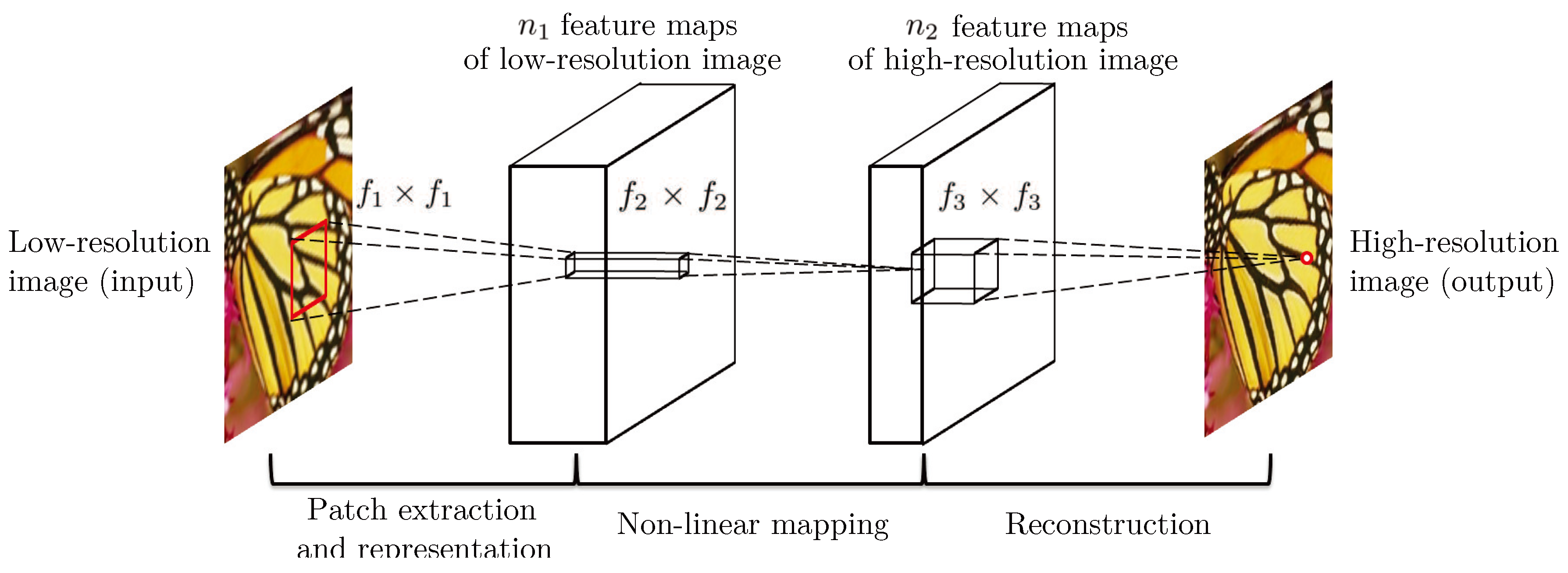
Figure 2.
A Model that uses a pre-trained loss network, courtesy of [10].
Figure 2.
A Model that uses a pre-trained loss network, courtesy of [10].
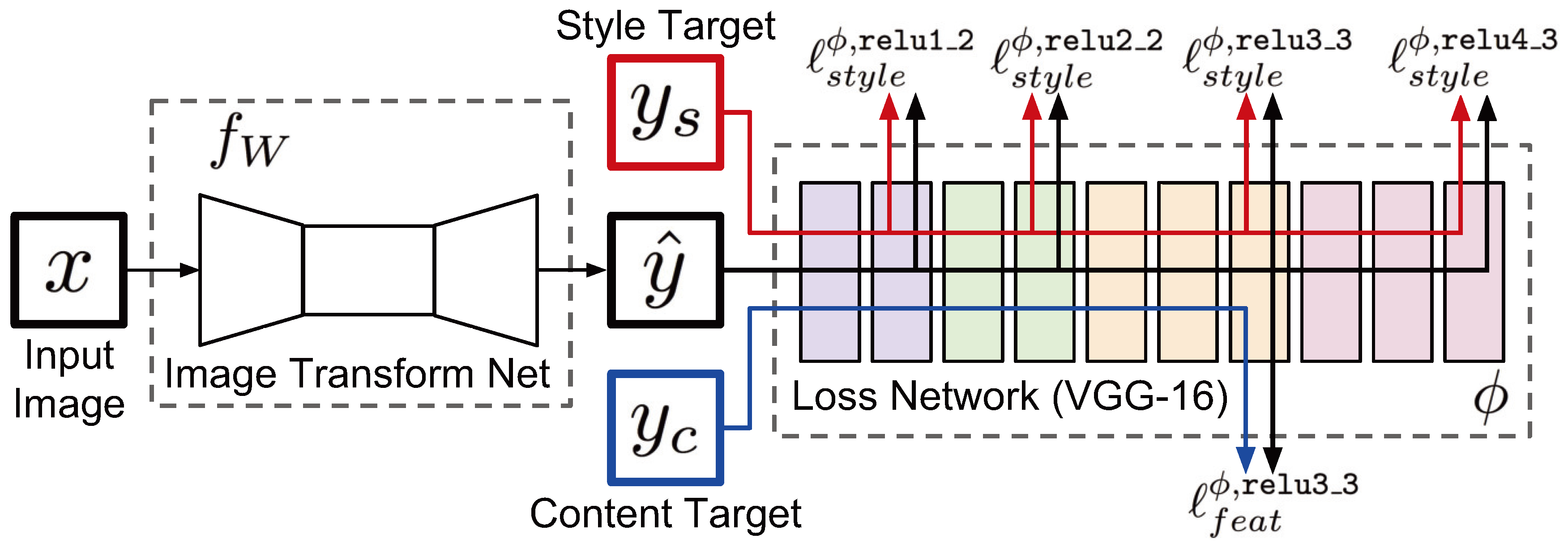
Figure 3.
SRResNet from
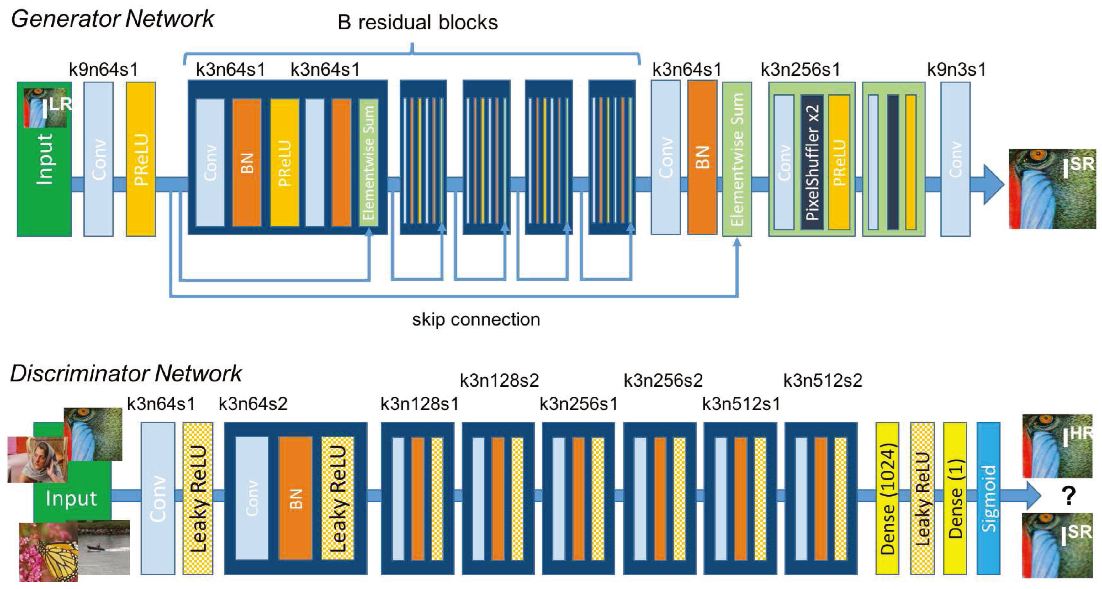
Figure 4.
Global Residual Learning: Reproduced from [17]
Figure 4.
Global Residual Learning: Reproduced from [17]
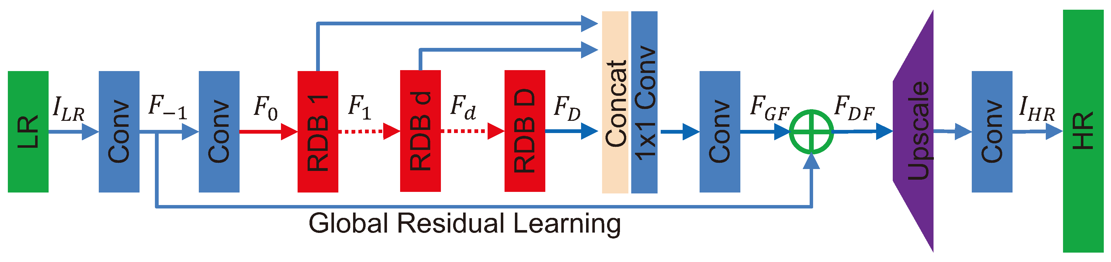
Figure 5.
Local Residual Learning: Reproduced from [17]
Figure 5.
Local Residual Learning: Reproduced from [17]
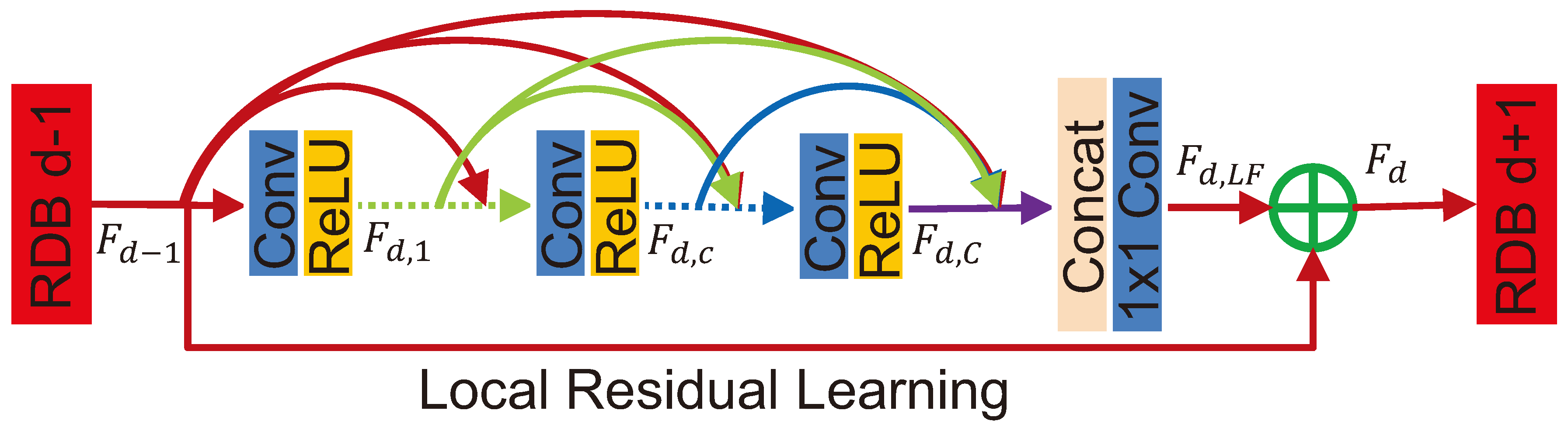
Figure 6.
Residual Channel Attention Network from [18]
Figure 6.
Residual Channel Attention Network from [18]
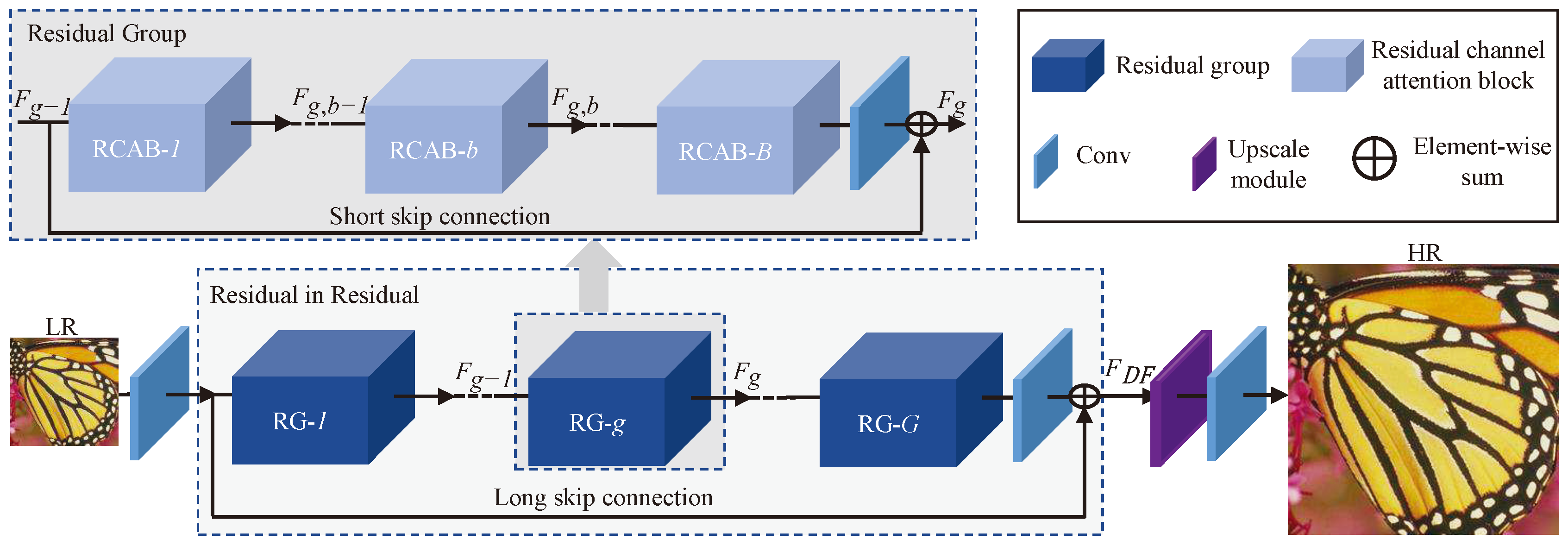
Figure 7.
Early Autoencoder Architecture
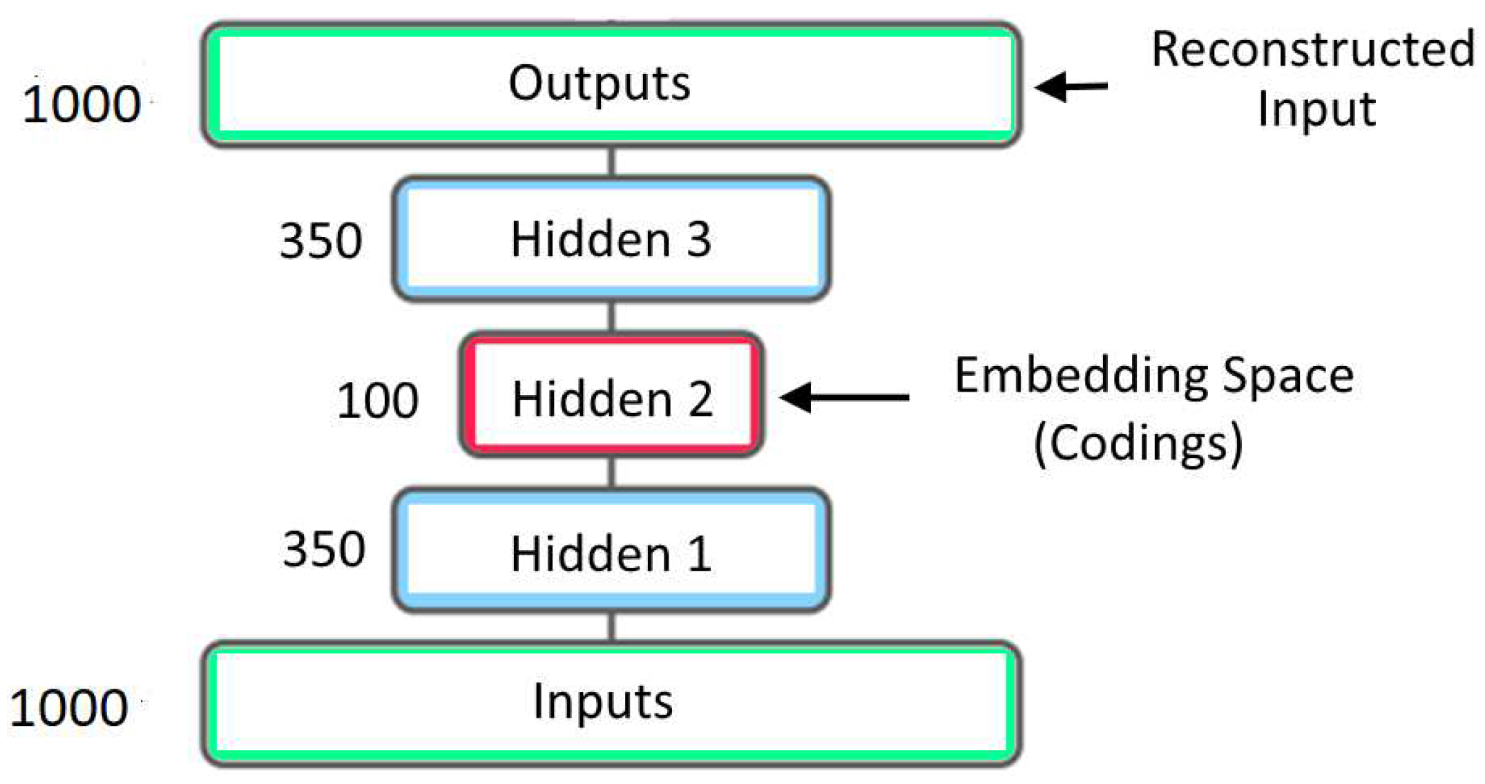
Figure 8.
Autoencoder used to reconstruct an image
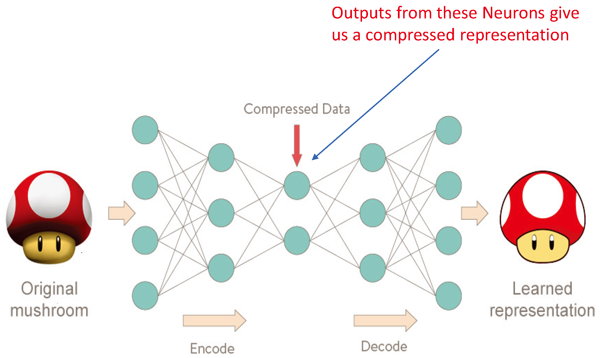
Figure 9.
Convolution: A moving image filter takes dot-products with a sub-matrix of the image and places the result in a new image called the featuremap.
Figure 9.
Convolution: A moving image filter takes dot-products with a sub-matrix of the image and places the result in a new image called the featuremap.
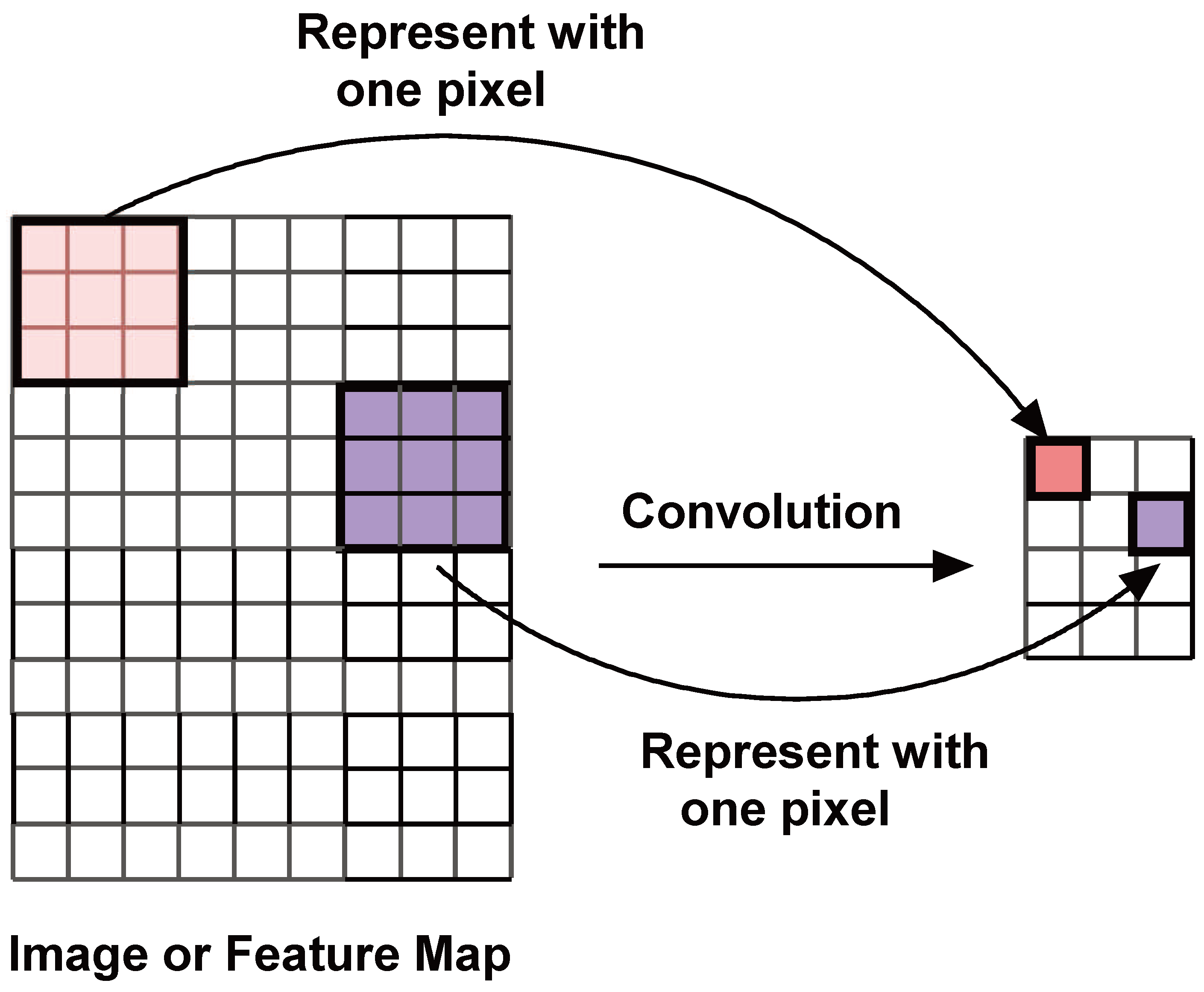
Figure 10.
Example of a Subsampling Operation: Maxpooling
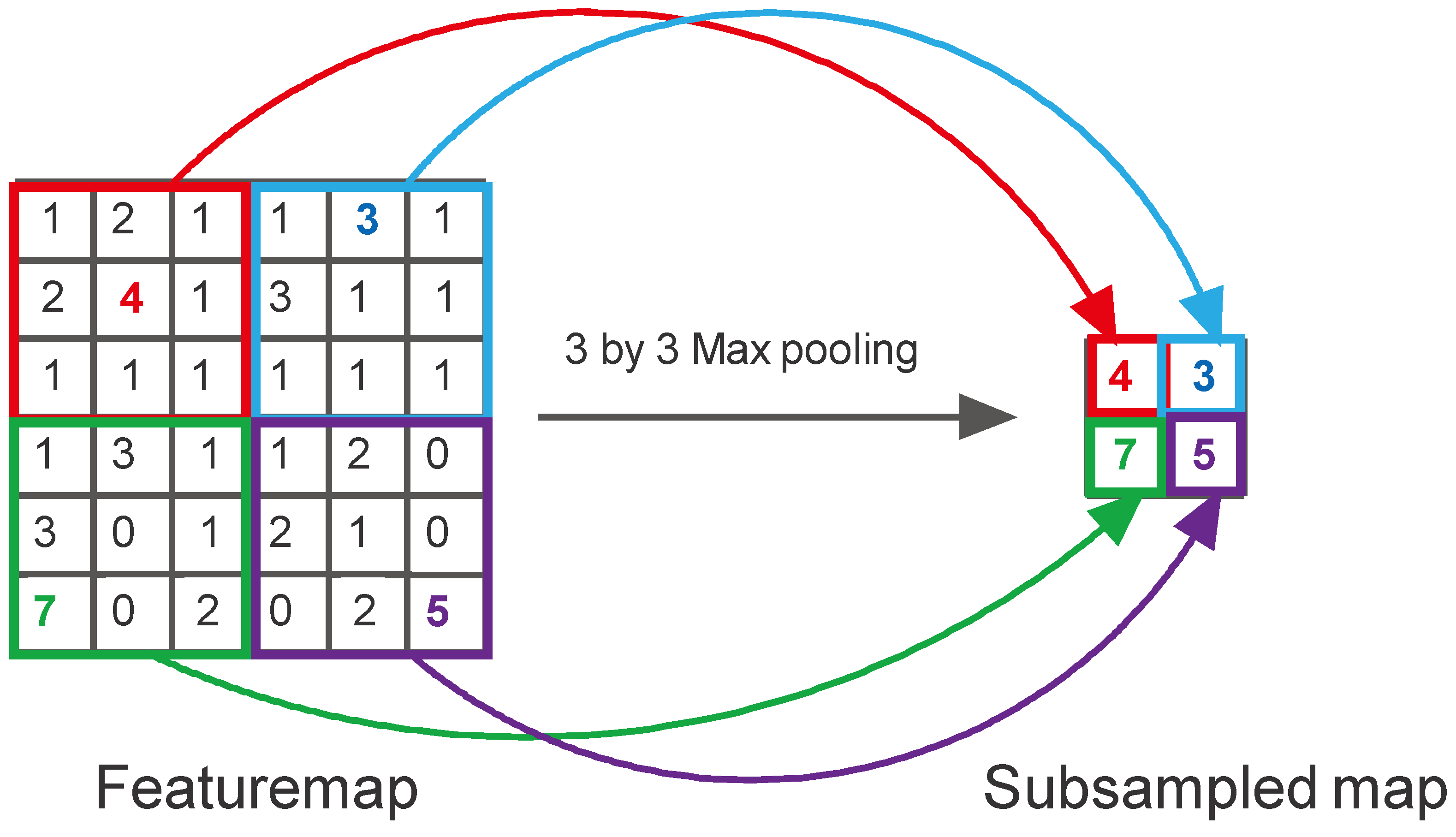
Figure 11.
A Simple CNN
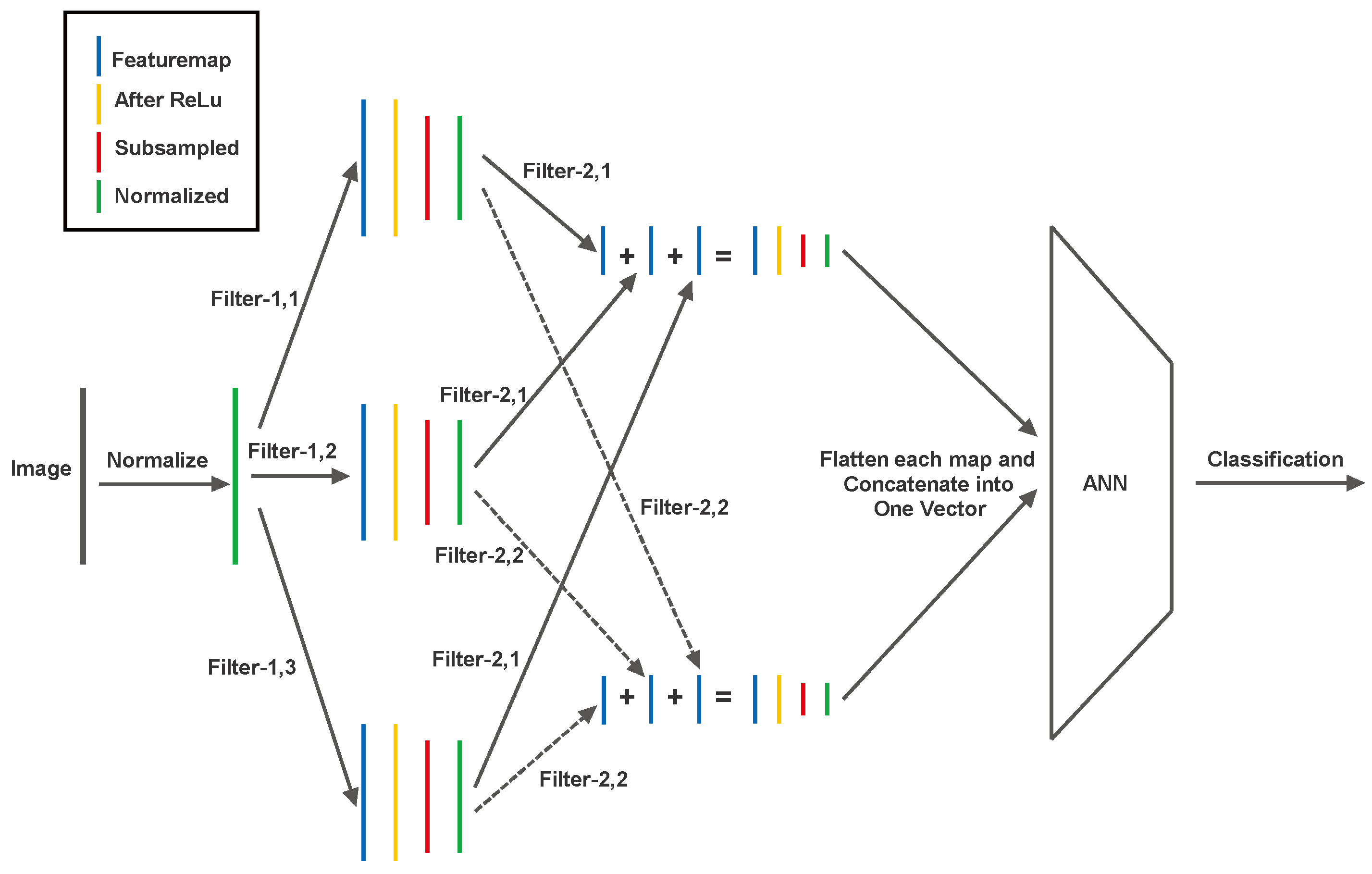
Figure 12.
Typical Autoencoder Structure
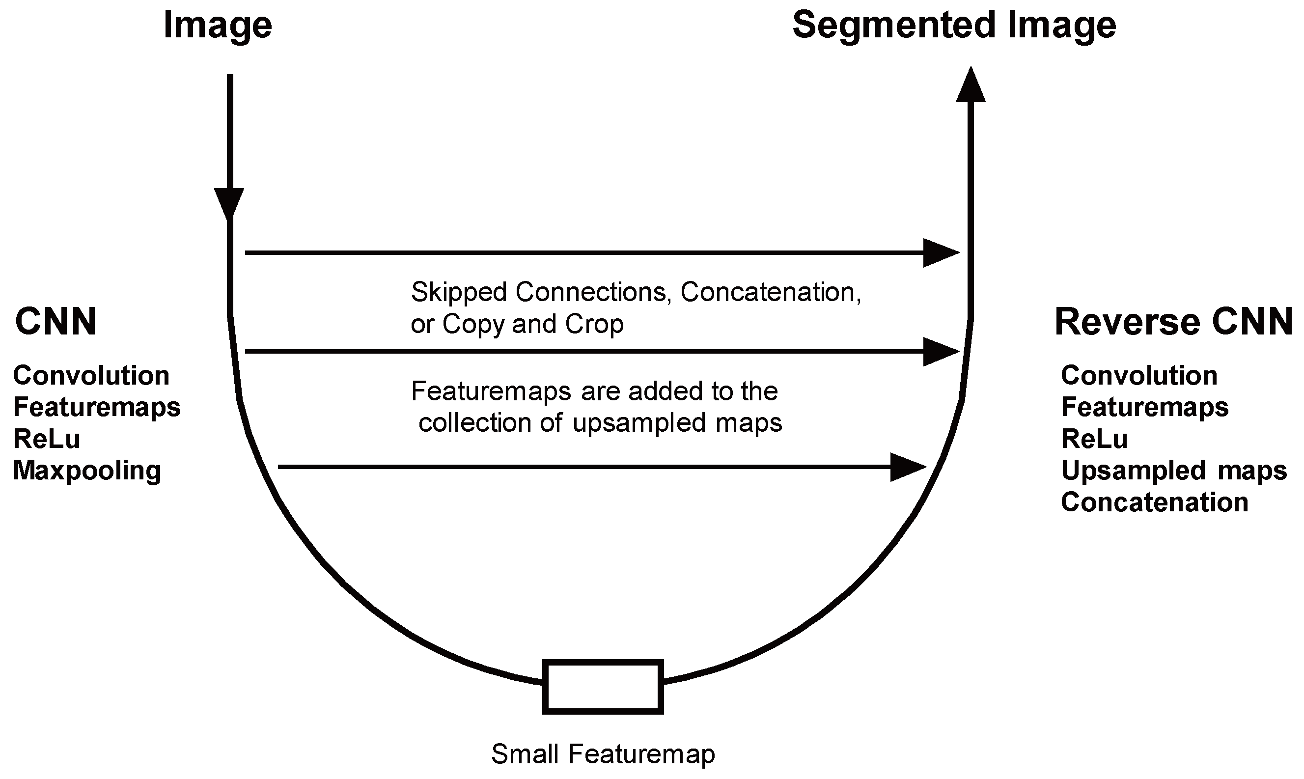
Figure 13.
Transpose Convolution.
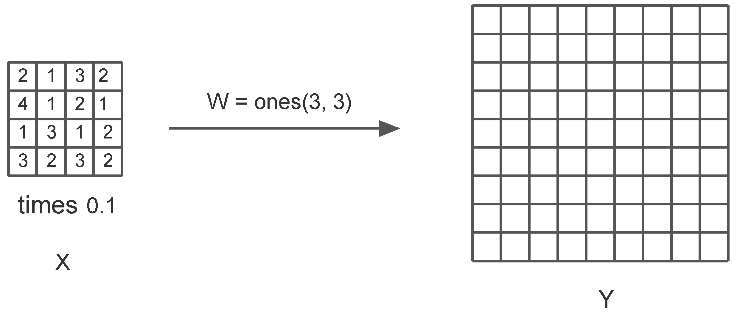
Figure 14.
Our Network Structure. Five Conv. layers that downsample the input image, followed by five Transposed Conv. layers for up-sampling, and one last Conv. layer for image reconstruction. Residual skip connections are not shown in this figure
Figure 14.
Our Network Structure. Five Conv. layers that downsample the input image, followed by five Transposed Conv. layers for up-sampling, and one last Conv. layer for image reconstruction. Residual skip connections are not shown in this figure
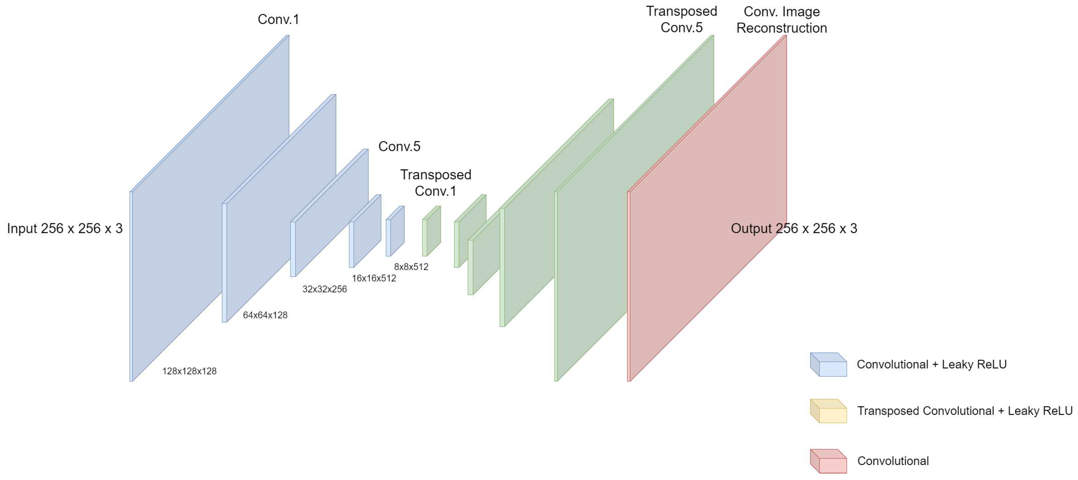
Figure 15.
Network Architecture with skip connections
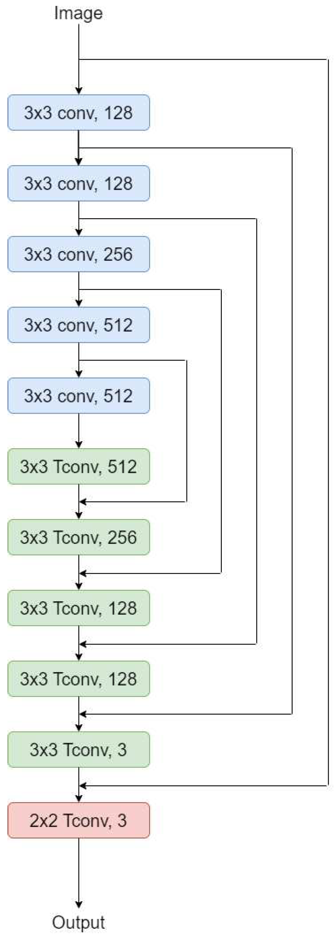
Figure 16.
High Resolution Ground Truth Image on the left, Low Resolution Input in the middle, and the High Resolution Output Image on the right.
Figure 16.
High Resolution Ground Truth Image on the left, Low Resolution Input in the middle, and the High Resolution Output Image on the right.
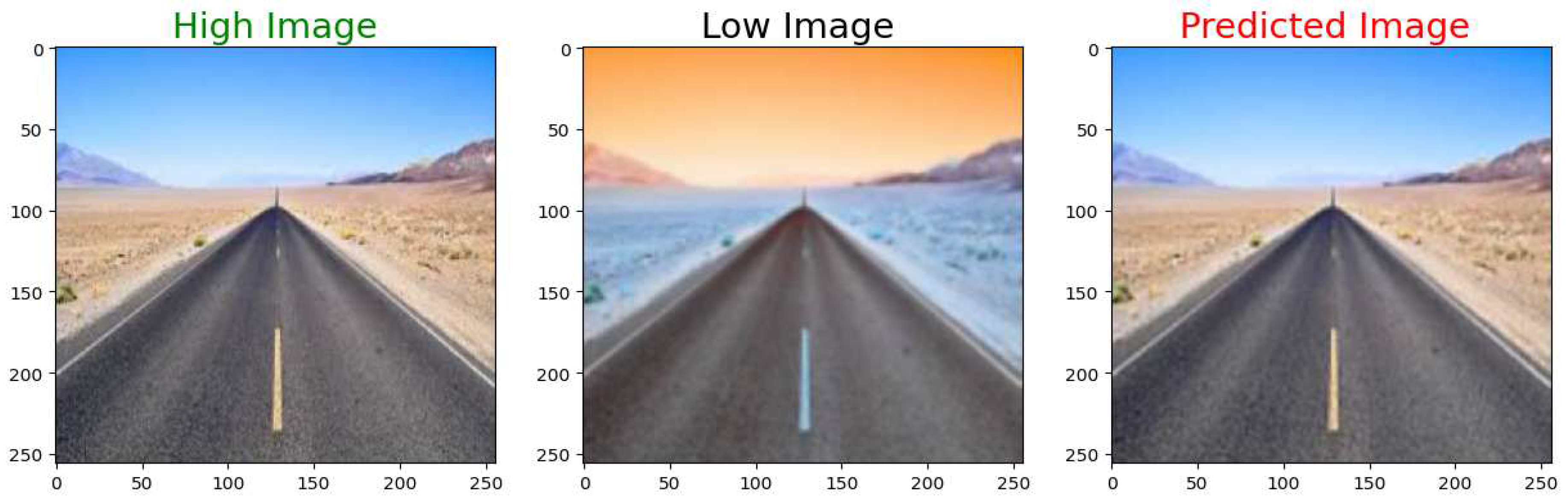
Figure 17.
High Resolution Ground Truth Image on the left, Low Resolution Input in the middle, and the High Resolution Output Image on the right.
Figure 17.
High Resolution Ground Truth Image on the left, Low Resolution Input in the middle, and the High Resolution Output Image on the right.
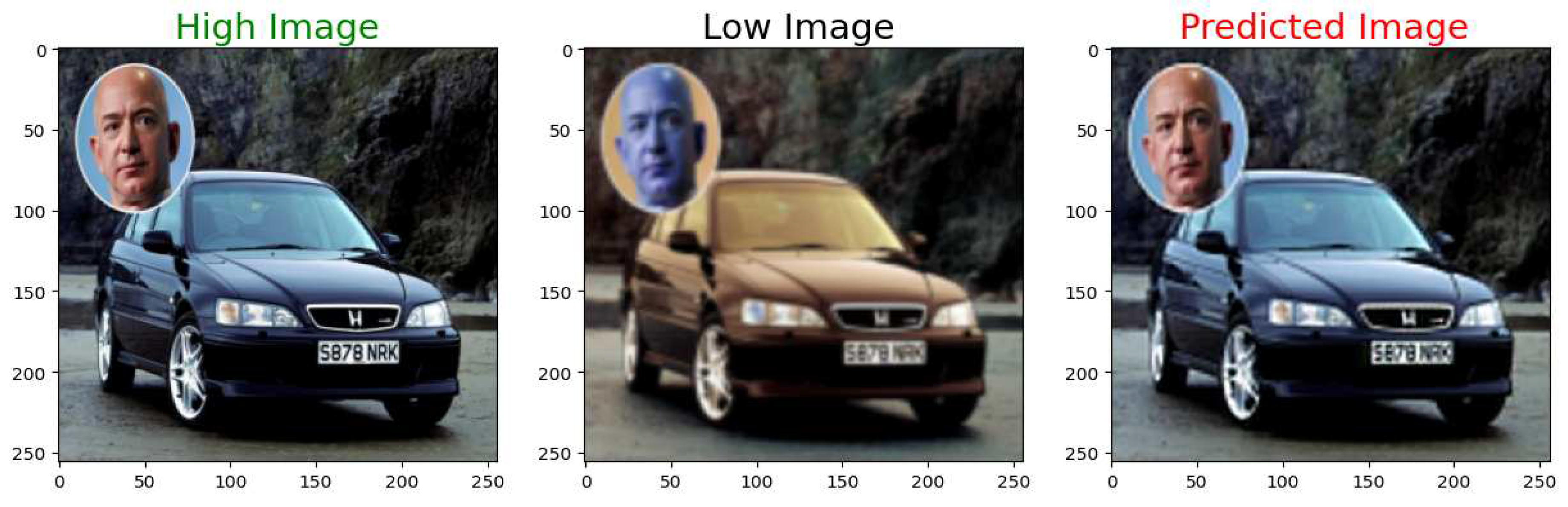
Figure 18.
High Resolution Ground Truth Image on the left, Low Resolution Input in the middle, and the High Resolution Output Image on the right.
Figure 18.
High Resolution Ground Truth Image on the left, Low Resolution Input in the middle, and the High Resolution Output Image on the right.
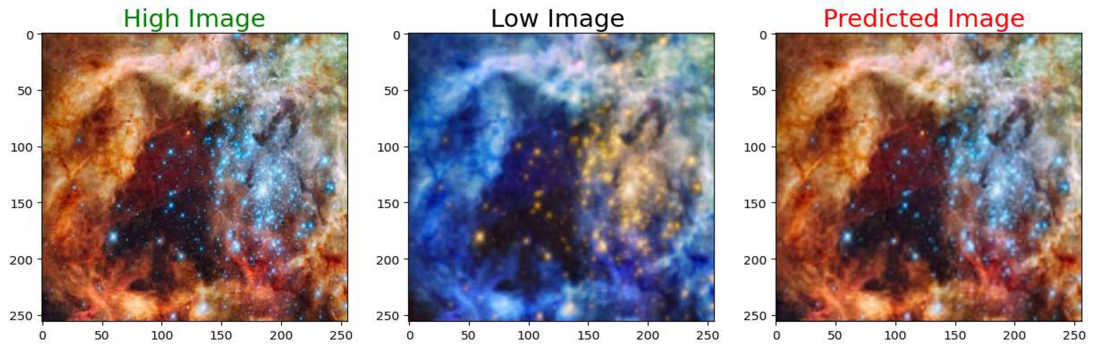
Figure 19.
High Resolution Ground Truth Image on the left, Low Resolution Input in the middle, and the High Resolution Output Image on the right.
Figure 19.
High Resolution Ground Truth Image on the left, Low Resolution Input in the middle, and the High Resolution Output Image on the right.
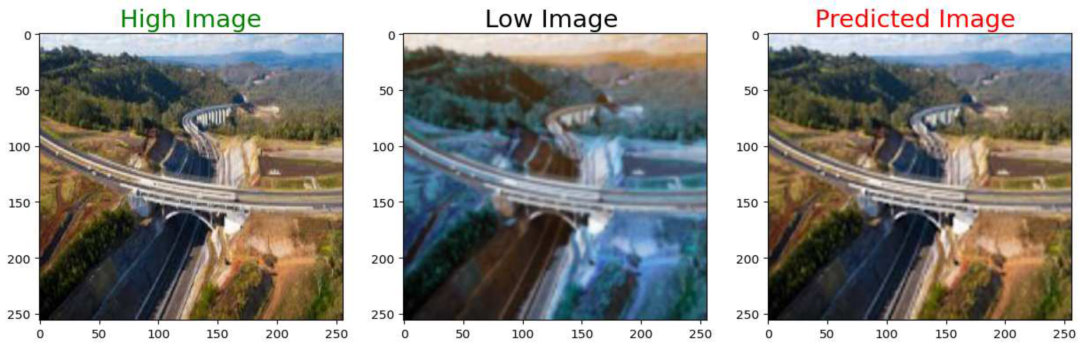
Figure 20.
High Resolution Ground Truth Image on the left, Low Resolution Input in the middle, and the High Resolution Output Image on the right.
Figure 20.
High Resolution Ground Truth Image on the left, Low Resolution Input in the middle, and the High Resolution Output Image on the right.
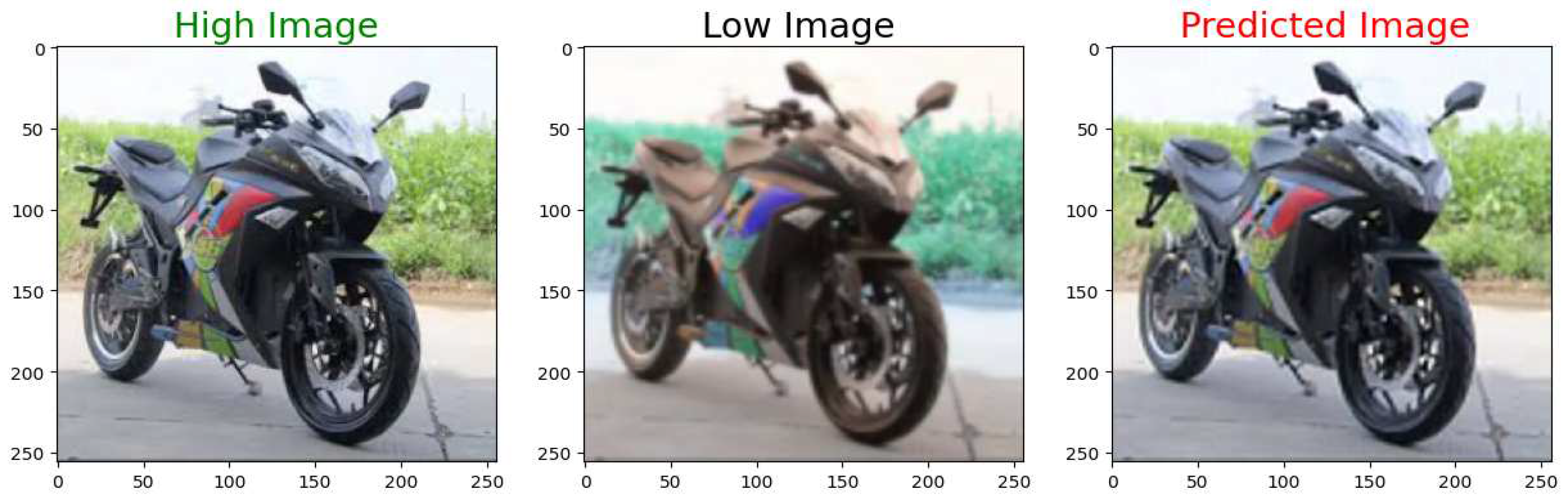
Figure 21.
High Resolution Ground Truth Image on the left, Low Resolution Input in the middle, and the High Resolution Output Image on the right.
Figure 21.
High Resolution Ground Truth Image on the left, Low Resolution Input in the middle, and the High Resolution Output Image on the right.
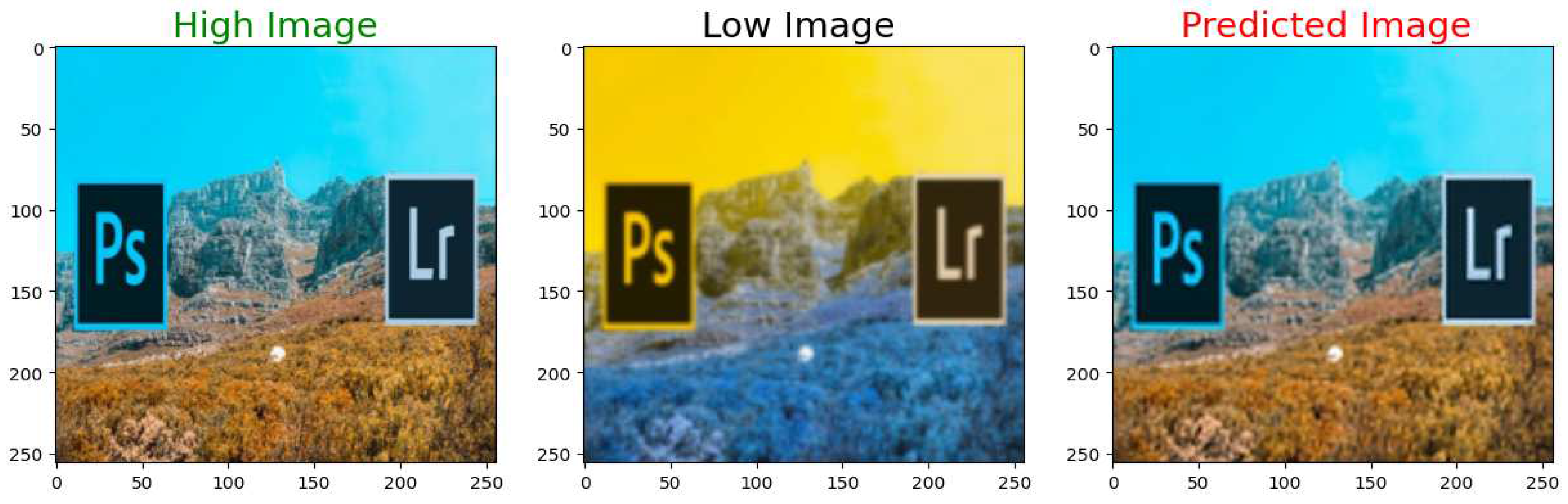
Figure 22.
High Resolution Ground Truth Image on the left, Low Resolution Input in the middle, and the High Resolution Output Image on the right.
Figure 22.
High Resolution Ground Truth Image on the left, Low Resolution Input in the middle, and the High Resolution Output Image on the right.
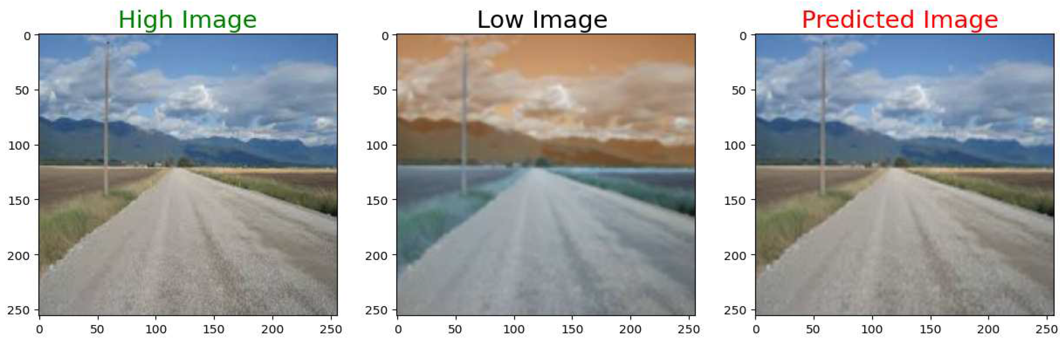
Figure 23.
High Resolution Ground Truth Image on the left, Low Resolution Input in the middle, and the High Resolution Output Image on the right.
Figure 23.
High Resolution Ground Truth Image on the left, Low Resolution Input in the middle, and the High Resolution Output Image on the right.
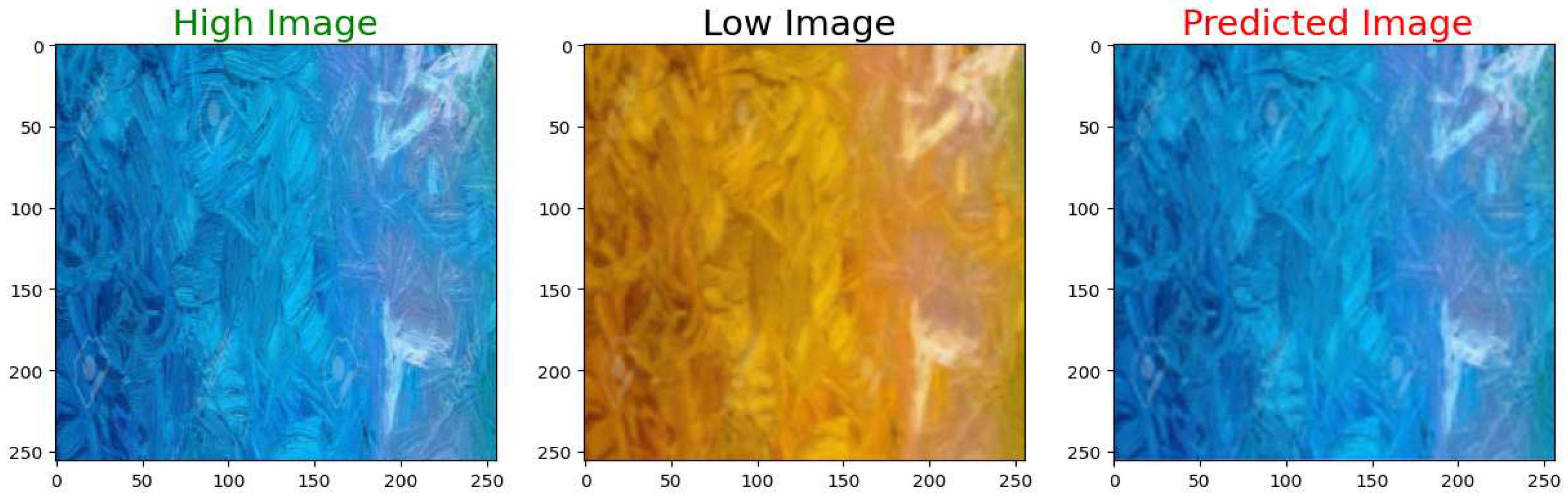
Figure 24.
High Resolution Ground Truth Image on the left, Low Resolution Input in the middle, and the High Resolution Output Image on the right.
Figure 24.
High Resolution Ground Truth Image on the left, Low Resolution Input in the middle, and the High Resolution Output Image on the right.
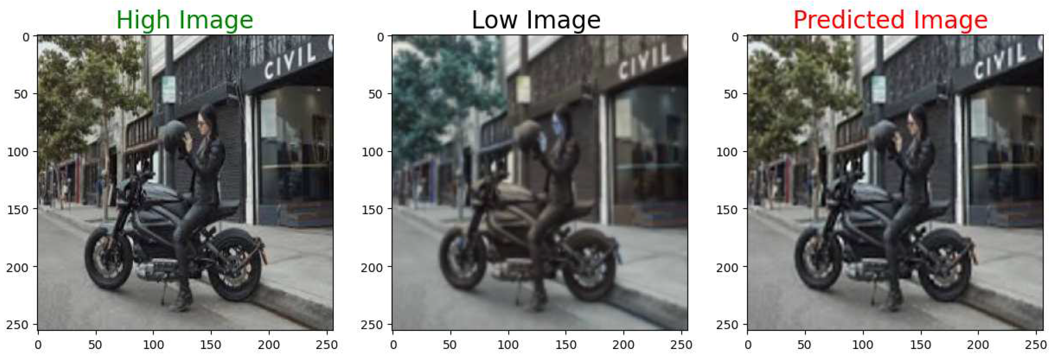

Table 1.
PSNR, MSE, and SSIM values for 9 testing images. These values obtained with 3x3 filters, 11 layers, 7 epochs, and 0.001 step size. Average values for PSNR, MSE, and SSIM are 76.40, 0.005, and 0.89 respectively
Table 1.
PSNR, MSE, and SSIM values for 9 testing images. These values obtained with 3x3 filters, 11 layers, 7 epochs, and 0.001 step size. Average values for PSNR, MSE, and SSIM are 76.40, 0.005, and 0.89 respectively
| PSNR | MSE | SSIM |
|---|---|---|
| 73.02 | 0.01 | 0.9 |
| 75.69 | 0.01 | 0.88 |
| 75.63 | 0.01 | 0.90 |
| 75.85 | 0.01 | 0.92 |
| 73.51 | 0.01 | 0.83 |
| 82.34 | 0.001 | 0.96 |
| 79.64 | 0.002 | 0.93 |
| 77.38 | 0.003 | 0.86 |
| 74.59 | 0.01 | 0.90 |
Table 2.
PSNR, MSE, and SSIM values for 9 testing images. These values were obtained with 3x3 filters, 11 layers, 7 epochs, and 0.0001 step size. Average values for PSNR, MSE, and SSIM are 72.76, 0.01, and 0.81 respectively
Table 2.
PSNR, MSE, and SSIM values for 9 testing images. These values were obtained with 3x3 filters, 11 layers, 7 epochs, and 0.0001 step size. Average values for PSNR, MSE, and SSIM are 72.76, 0.01, and 0.81 respectively
| PSNR | MSE | SSIM |
|---|---|---|
| 70.51 | 0.02 | 0.81 |
| 72.50 | 0.01 | 0.78 |
| 72.50 | 0.01 | 0.81 |
| 71.95 | 0.01 | 0.84 |
| 69.78 | 0.02 | 0.68 |
| 77.90 | 0.003 | 0.93 |
| 75.25 | 0.01 | 0.88 |
| 72.75 | 0.01 | 0.76 |
| 71.75 | 0.01 | 0.81 |
Table 3.
PSNR, MSE, and SSIM values for 9 testing images. These values were obtained with 3x3 filters, 11 layers, 20 epochs, and 0.001 step size. Average values for PSNR, MSE, and SSIM are 75.76, 0.01, and 0.91 respectively
Table 3.
PSNR, MSE, and SSIM values for 9 testing images. These values were obtained with 3x3 filters, 11 layers, 20 epochs, and 0.001 step size. Average values for PSNR, MSE, and SSIM are 75.76, 0.01, and 0.91 respectively
| PSNR | MSE | SSIM |
|---|---|---|
| 73.98 | 0.01 | 0.92 |
| 75.34 | 0.01 | 0.89 |
| 76.07 | 0.004 | 0.92 |
| 75.41 | 0.01 | 0.94 |
| 73.16 | 0.01 | 0.86 |
| 79.86 | 0.002 | 0.97 |
| 77.54 | 0.003 | 0.94 |
| 75.36 | 0.01 | 0.83 |
| 75.09 | 0.01 | 0.92 |
Table 4.
PSNR, MSE, and SSIM values for 9 testing images. These values obtained with 3x3 filters, 11 layers, 20 epochs, and 0.0001 step size. Average values for PSNR, MSE, and SSIM are 78.25, 0.003, and 0.93 respectively
Table 4.
PSNR, MSE, and SSIM values for 9 testing images. These values obtained with 3x3 filters, 11 layers, 20 epochs, and 0.0001 step size. Average values for PSNR, MSE, and SSIM are 78.25, 0.003, and 0.93 respectively
| PSNR | MSE | SSIM |
|---|---|---|
| 74.47 | 0.007 | 0.93 |
| 77.24 | 0.004 | 0.92 |
| 77.35 | 0.004 | 0.94 |
| 78.09 | 0.003 | 0.95 |
| 75.02 | 0.006 | 0.89 |
| 85.10 | 0.001 | 0.98 |
| 81.87 | 0.001 | 0.95 |
| 79.05 | 0.002 | 0.90 |
| 76.05 | 0.005 | 0.93 |
Disclaimer/Publisher’s Note: The statements, opinions and data contained in all publications are solely those of the individual author(s) and contributor(s) and not of MDPI and/or the editor(s). MDPI and/or the editor(s) disclaim responsibility for any injury to people or property resulting from any ideas, methods, instructions or products referred to in the content. |
© 2023 by the authors. Licensee MDPI, Basel, Switzerland. This article is an open access article distributed under the terms and conditions of the Creative Commons Attribution (CC BY) license (http://creativecommons.org/licenses/by/4.0/).
Copyright: This open access article is published under a Creative Commons CC BY 4.0 license, which permit the free download, distribution, and reuse, provided that the author and preprint are cited in any reuse.


