

Submitted:
02 November 2023
Posted:
03 November 2023
You are already at the latest version
Abstract
Tablets are the most used solid dosage form in medical treatments. The realistic modeling 1 of such specific object shapes in computer simulations has been demonstrated already by the author 2 for bi-convex round tablets but needs to be extended for a wider range of tablet shapes. Moreover, 3 the number of tablets must be large enough to simulate industrial drum coaters, which are typically 4 used for film coating processes. Whilst this long lasting process where tablets flow continuously, 5 tablets are loaded by frequent changes of individual contacts. Using a tailored simulation tool named 6 pharmAssist , written for GPUs (modern massively parallel processors in graphics cards and HPC 7 accelerators), we implemented the widely used oblong tablet shape. We are able to simulate flows 8 involving industrial scale number of such tablets. Data mining allows for statistical analyzis of 9 pair-wise contacts of different geometric features. Our simulation results serves as an observation 10 space, which cannot be addressed by experimental analyzis and will help to avoid degradation of 11 tablets like chipping or other defect phenomena. This paper reflects current development work in 12 order to extend the DEM with a new shape class, which comprises the modelling of compacted or 13 extruded objects, which have a smooth exterior, a flat band and sharp contour edges
Keywords:
DEM
; drum coating
; mixing
; tablet shape
; digital twin
; GPU
1. Introduction and Motivation
1.1. DEM contributions
Many anhancements of the Discrete Emlement Method (DEM) are already achieved over the years. Starting with two-dimensional simulations of some hundred particles in the early 90th, nowadays threedimensional simulations are standard. Most of them are using spherical particles.
A leapfrog enhancement of DEM was possible with CUDA programming environment for the Graphics Processing Unit (GPU) [1]. This allowed to enter the million range using regular workstations [2]. Suggestions to the authors PhD mentor M. Kuna in 2010 resulted in a particle shape definition for polyhedra [3], adapted to GPU computation by E. Siegmann lateron [4].
The acceptance of digital twin tools depend on their capabilities to reflect real world problems. It is important to develop simulation tools which are capable to model realistic content. Here, in our current study, we focus on the shape of pharmeceutical tablets.
1.2. Tablet Coating
Unit Operation: Pharmaceutical tablet coating is a process used to apply a coating layer to a tablet to improve its appearance, taste, stability, and ease of swallowing. Tablet coating also helps to mask the unpleasant taste and odor of certain drugs and protects the tablet from moisture and light.
The tablet coating process involves several steps, which can vary depending on the type of coating and equipment used. Here is a general overview of the process:
Preparation: Before coating, tablets must be prepared by cleaning and polishing to remove any impurities or residues from the manufacturing process. Mixing the coating solution: The coating solution is prepared by mixing the coating material (usually a polymer) with solvents, plasticizers, and other additives. The solution is mixed until it is homogeneous and has the desired viscosity and density.
Coating application: The coating solution is then applied to the tablets using a coating machine. There are several types of coating machines available, including pan coaters, fluidized bed coaters, and spray coaters.
Drying: After the coating is applied, the tablets are dried to remove the solvents and other volatile components from the coating solution. This step is critical to ensure the uniformity and integrity of the coating.
Polishing: After drying, the tablets may be polished to improve their appearance and remove any rough edges. Overall, pharmaceutical tablet coating is a complex process that requires careful control of various parameters, including the type of coating material, coating thickness, and drying time, to ensure the quality and consistency of the coated tablets.
1.3. DEM - specialized for Pharmaceutical Processing
In the last decade DEM simulations have been widely used to analyze flows of granular media with the main emphasis on flows where the interaction between particles and a fluidic phase can be neglected. Extensions for extensively used industrial processes which are involve liquid spray modeled by ray-threading technique, for example film coating, dry impregnation and resulting wet imbibition, were invented and added successfully already by the author together with Rutgers Catalyst Consortium research group [5]. Here, liquids are handled implicit by altering friction, particle mass or by mimicking of liquid bridge force effects; Only particle-particle contacts are considered for mechanical interaction. The describes implementation works in-place, so whilst simulation runtime, properties (liquid content, particle mass, friction coefficients or cohesive forces) can change and alter the granular flow. Another approach to simulate spray is a kind of a droplet fog, shown in [6].
In contrast to well established simulation methods like FEM and CFD, DEM does not allow refinded regions for more detailed resolution. Often narrow slits or tiny gaps dictate the minimum particle size which has to be used all over the simulation volume. Moreover, users whom want to incorporate complex shaped particles have to choose between the number of particles and an acceptable simulation time which is lowered in most cases; Even though, a promising extrapolation approach can speedup many simulations significantly [7]. But in realistic pharmaceutical unit operations the number of tablets or capsules often surpass the million range in terms of particle numbers. This makes it even harder to incorporate geometrical details. Many promissing approaches for true shape particle modeling are covered by [8,9,10,11].
Some approximations toward tablets were carried out with superquadrics [12], [13]. But all of the flexible shape featuring superquadric objects have only smooth rounded edges. In the work of Yu et al., flat cylindical sharply edged objects are introduced [14]. The first true shape modeling approach for bi-convex tablets in 2D were found in the work of Song et al. [10]. Wassgren et al. demonstrated a lab-scale simulation study of bi-convex tablets [15]. Based on Song et al., the author and H. Kureck developed a 3D model and described the implementation in [16], which is tailored for GPU computing and runs similar fast than the simple sphere approach!
1.4. pharmAssist DEM
In order to be able to simulate large granular systems, a high-performance DEM code was developed based on CUDA technology [18,19]. pharmAssist can simulate millions of particles on inexpansive GPU hardware as well as on any available Pro-Series Nvidia GPUs. It is a family of code packages of the so called "assist’s".
1.5. Numerical Precision
In order to serve the common double precesion capability of current GPU generations by one code base, the code is built using a ’guarded type definition’ of type real which unfolds to either type float or double together with all CUDA toolkit definitions of data types make_eal?() accordingly (?=).
1.6. Visualization
DEM particle simulations in the million-particle range are still a challenge today but already common in some research groups. Vizualisation capabilities have to keep pace. Therefore, all available shapes (spheres, ellipsoids, polyhedra, capsules and tablets) have a shader-based rendering in our vizualisation tool. Our Kivy-based Pre- and Postprocessor has been tested to remain interactive up to several millions of particles on single a graphics card (Vizualisation presented in this paper was performed on a Nvidia RTX2080Ti using the VizAssist tool. Kivy is a crossplatform User Interface and supports also mobile devices running IOS or Android.
2. Implementation
2.1. Numerical Model
The wide spreaded ’soft’ particle approach is used in our work where spherical particles exert forces due to their mass m and geometrical overlap at the contact points c. The total force F and torque M acting on a particle
is the summation of all contact forces with other particles or boundaries and the gravitational force. By consideration of Newtons second law at time t, we obtain the acceleration which can be used for an explicit time step integration scheme with a time step in order to obtain the new velocities and corresponding positions for each particle in the system. Here, the classical Verlet integration scheme is employed for positions [22]
Velocities are obtained by central difference approximation
The DEM accounts for translational as well as for rotational degrees of freedom. Both are handled separately by the application of the Verlet algorithm (3 - 5) and an Euler integration (7) in the latter case. Total torque M and moment of inertia I are used to obtain the angular acceleration
and the new angular velocity at time
In order to obtain the new particle orientation an integration of the angular velocity is performed. Here, is a quaternion representation of particle orientation, see [23]. Details of the more complex implementation of a corrector-predictor method used in pharmAssist, can be found in [24].
The force laws in normal and tangential direction of our im[plementation follow the guidance of S. Luding, see [25]:
where is the static Coulomb friction coefficient, , are spring constants and , account for viscous damping in normal and tangential direction respectively. The cohesive force is only active, if cohesive forces are considered, e.g., in the case of liquid bridges. The tangential overlap
allows for restoring forces if the contact had existed already in the previous time step.Therefore, the evolution of the tangential overlap can be written also as
In the algorithm, where the time of the lasting contact is discretized by k time steps dt
The reason for keeping the spring history by integration over contact time is to achieve tangential elasticity. Without tracking the evolution of it is impossible to reach a finite force where the tangential velocity [26]P.13ff,[27],Ch.4ff. Tangential elasticity is a sufficient condition in order to simulate quasi-static and static granular flows. There, a particle assembly is moving with less granular temperature or it is resting, in both cases with respect to gravity. Quasi-static granular flows capture the most physical processes like mixing, compaction, filling and storage of granular matter. Without tangential elasticity a particle assembly cannot withstand gravitational forces by traction. It would be unstable until interlocking is taking place, which can –moreover– not occur when the particles have a pure spherical shape.
Sliding friction, a rolling resistance and twist spin about the contact normal vector is implemented in analogy. Collisions between particles and STL walls are handled in a similar fashion, comparable to the particle-particle collisions case [23].
2.2. Parallelization and Implementation
The pharmAssist code employes the common cell-space logic, a regular subdivision of the simulation volume into cubic cells [28]. This allows a fast detection of the adjacent neighbors, because the search for particles is restricted to a volume within a cell. While the search time for selecting two entities from a set of N entities is of , the cell space logic has a linear growth characteristic of operations only. This is very important for DEM simulations when particle numbers exceed a few thousand. The cell-space implementation is tolerant in terms of particle size. Particles with an arbitrary size distributions within a limit of about 1:5 can be simulated without remarkable performance loss. Classical particle in cell (PIC) codes run a huge for-loop over the cells around a particle, collecting neighboring forces and integrating the resulting acceleration to obtain new positions and velocities.
A tree algorithm for STL handling follows the reference implementation with modified aligned bounding boxes for static, dynamic and free floating arbitrary shaped STL geometries (coating drums, railway sleepers, dummy objects etc) [29].
Method: Our software redefines the concept of parallelization of DEM with strong regards to the GPU capabilities. The light weight threads technology offered by programming models like Nvidia CUDA or AMD HIP allow for the simultaneous execution of up to hundreds of millions of such threads [19,30]; Morover, it is often required in terms of utilization of the potent hardware which fosters Teraflop performance.
Domains: Where domain decomposition of the cell-space is the common parallelization strategy on multi-CPU systems, where the simulation volume is divided into equal sized partitions for each of the CPU cores. The number of threads is equal to the number of domains. Such a coarse approach does not work on GPUs. Therefore, software cannot be simply ported to GPU, it has to be rewritten in total.
Thread-per-cell: The first good fitting approach is the split of the simulation volume into subsets of cells of the cell-space. Here, each cell is assigned to its neighborhood of 3x3x3 cells. Then, each of the cell is assigned to one thread and is ’looking’ for surrounding cells and contacting particles therein. So the number of threads is equal to the number of cells, typically reduced to the number of particles because N particles can only occupy a maximum of N cells (the particle center location defines the belonging). But on polydisperse systems number of particles per cell increases and performance is wasted in looping and search for more much than 3x3x3 particles in the latter case.
Thread-per-particle: This approach already allows a fast execution of the contact force computation but the varying number of contacts leads to unpredictable execution times for each of the thread-per-particle assigned threads (the one incorporating the most contacts delayes the execution of a whole threadblock). Typical contact numbers ranging from 0 – 8 contacts for each particle.
Thread-per-contact: Here, the situation is similar to the previous approach but a search step, which builds up a list of true contacts, is placed at the beginning of each of the time-steps. After the detection of contact pairs the contact list is prepared for seperate execution in a one-thread-per-contact implementation. As a result of an average of 5 – 8 contacts per particle (and many more blind contacts, when the bounding sphere of a non-spherical particle declares a potential contact) and the overhead of the blinds, twenty million up to hundred million threads are running in parallel for a simulation with a moderate size of only one million to five million particles.
2.3. Oblong Tablet Shape
Due to the manufacturing process in tablet press machines, most of tablets have a smooth cylindric section alongside the compaction axis, the so called band. The oblong shape of a tablet is characterized by a circumferending band with opposite parallel sections at the long sides, see Figure 1.
Some tablets land on their band and stand on the plane which one can observe in Figure 1. Here, two out of around thirty tablets stand upright. Such rather simple effects can only be reflected in particle simulations, when geometry features of the particles are modeled accordingly. In Figure 2 a similar simulation case of some tablets are dropped onto a rigid plane under gravity shows comparable behavior (25 out of 455 tablets land upright).
The geometry definition we use in the present work is an extension of the simple but smart idea of Song et al. [10], outlined in Figure 3. We extend this approach by adding a further L-parameter, namely . Where , and are corresponding to band hight, total hight and band width of the tablet, in the oblong shape extension represents the band lenght or total length of the oblong tablet. A fix set of the shape parameters defines an oblong tablet shape. Thereafter, such a tablet can be scaled using one size parameter only, see Figure 3.
The main idea of oblong particle shape definition is to use the bi-convex Song-tablet in Figure 3 as countour shape object (CSO). A contour shape is created by moving around such a geometrical defined CSO. Very similar to spherocylinders, which form by shifting a perfect shpere along a line, see Figure 4. Details of spherocylinder collision are given in [31]. This shape serves to model pharmaceutical capsules. In short, the collision between two capsules is handled by the collision of the two spheres at the position where both capsule axes are having its shortest distance.
When we simply replace the sphere in Figure 4 with a bi-convex tablet, shifting along the capsule axis, the oblong tablet shape is created, see Figure 4. Whereby the spherocylinder forms round caps at both ends the oblong tablet instead has ends of exactly the shape of a half bi-convex tablet.
All pairwise contact conditions for the oblong shaped tablets remain the same than for pairwise bi-convex tablet collisions, explicitly given in [16].
3. Basic Application Example
3.1. Experimental Device
We use a rotating drum for our simulations, sketched in Figure 7, which is widely used in unit operations in pharmaceutical processing or food industries such as tablet coating or pan coating candy production. Drum coaters have been investigated to great extent for non-spherical particles by Hlosta et al. [32]. Their findings regarding fill levels depending on the asphericity of particles helped us to set up our simulation case.
In this synthetic case study we use an STL-based geometry of an empty drum without baffles or scrapers. The drum is filled up to 40% filling height with 320.000 oblong tablets, shown in Figure 7. The total mass of the batch is 160kg.
3.2. Simulation Setup
In order to study the influence of drum speed to the contact pair statistic, four different simulations have been ran. This simulations ranges from 6rpm to 18rpm and were carried out as shown in Figure 8.
For all cases from 6 rpm to 18 rpm, the simulation ran for 10 seconds. So our cases made 1, 1.5, 2 and 3 revolutions resp. The tablet size was 8.6 mm radius ( in Figure 3). The shape defining set for a unit tablet with a length of 1 is given by . Using this dimensions we obtain a tablet mass of 500mg.
Simulation parameters are given in Table 1.
4. Results
4.1. Contact tracking
In order to get a data base for statistical analysis of frequency of the occurance of contacts, we have markers in the simulation code which are written for each contact pair and which are summarized for each contact type. Whilst the simulation run, every 0.1s the histograms data are stored.
4.2. Contact pair statistics
Simulations allow to access data not available by experimental means at all. Having complex shaped tablets available, we decided to make a classification on different parts (cap, band rim) of an oblong tablet, depicted in Figure 5. The resulting six contact pair combinations are counted at time step intervalls of 0.01s. We labeled the pairs band-band, band-cap, cap-cap, rim-band, rim-cap and rim-rim. The histogram data are computed in-processing on the GPU and have no significant influence of the total performance.
All histograms in Figure 9 and Figure 10 are arranged as stacked barcharts, so one can compare the evolution of different contact pairs.
Different evolutions of contact pair variability can be observed up to four seconds of drum operation, cauesed by the different rpm of the drum in each case. Higher rpm values leads to higher fluctuations after the drum starts to operate. From four seconds onwards the evolution is steady with no remarkable visual differences between the cases running 6 rpm to 12 rpm. One can observe that cap-cap pairs dominate; followed by rim-cap pairs. The probably most damage causing rim-rim contacts are very low in all cases (around 2%). The fastes case has not reached steady pair distribution yet. The black, red and green pairs show an ongoing shift within each other. In contrast, all pairs with rim involved (upper three colors), are already steady after three seconds of simulation, see right diagram in Figure 10.
In order to reach better comparison, we plot data after the 10 seconds together in one diagram, see Figure 11. Now some interesting findings occur when we compare how the situation evolves with increasing drum speed in terms of their frequencies (comparing heights of the same colored sections). The absolute %-values for each of the pair frequencies are provided in Table A2.
Tendencies of the contact pair variability are summarized in Table 2. Further enhancement of the statistics might involve contact forces multiplied by contact duration or collision frequency, in order to describe wear depending on contact pairs etc.
4.3. Performance
The presented simulations (320.000 oblong tablets) ran for 10 seconds with a speed of 155 steps/s. Wall clock time to reach the 10 seconds was 1.8h, SP@RTX2080Ti). ( 121 steps/s DP @GV100). A comparable case with 1 Million oblong tablets ran with 41 steps/s DP@GV100, see also Table A1.
5. Industrial Scale Application
Coating processes as a pharmaceutical unit operation for bare tablet cores typically ran up to several hours. Whilst processing, the tablet bed is countinuously mixed in radial direction caused by circulation of tablets between the free surface of the bed and the cylinder wall. In order to enable axial mixing along the drum axis, multiple baffles are placed around the inner wall of the drum. The so improved mobility of the tablets decreases unwanted twinning, an effect where freshly coated wet tablets leaving the spray zone and stick together with another tablet, breaking up lateron again and remain coating film imperfections. For the mitigation of wetting effects, hot air streams through the tablet bed, shortening the drying phase. Therefore, the walls of such drum coaters are completely perforated like screen door windows. Together with the flow through property the perforation leads to a nearly frictionless transport of tablets by the moving drum wall, reflected by a high friction value (table ). Neither airflow, heating and spray are considered in the presented simulation case.
The used device geometry of the industrial simulation case is approximated to real devices which oparate batch sizes in the hundreds of kg range. The shape of the baffles is usually patented and therefore also simply visually adapted in the spirit of having smoothed internals guiding gently the tablet flow, see Figure 12.
Whilst mixing, the contact type pair statistic is recorded in order to evaluate the situation after steady state is reached.
In Figure 14 the pair-wise interaction frequency is depicted as it evolves over simulation time. The dominant pair is the cap-cap contact followed by band-band and rim-cap contact pairs. Less frequent are band-cap and rim-band pairs, rim-rim pairs are least frequent but can be most harmful with regard to shape degradation like edge imperfactions and notches.
Each granular assembly is characterized by its number of contacts between the granules. The so called coordination number C. In our case, oblong tablets are the individual objects, which interact by inter-tablet forces throughout these contacts. Where monodisperse spherical granular packings are known to have coordination numbers of about C = 5-6, the elongated tablet shape has higher coordination numbers ranging between C = 7-8, shown in Figure 15.
Bounding sphere contacts are potential contacts which are evaluated in the contact force computation part of the simulation code. Over 50 % of the contact calculations effort are wasted but are unkown to rasult in a true contact upfront the computational task. In the discussed case the total inter-tablet contacts are larger than 18 millions and the blind contacts caused by the bounding sphere detection reaches 50 million total contacts to compute in each individual timestep.
In order to get a more detailed analyzis of the acting inter-tablet forces, we give a summary of the probability density split into the six contact pairs, shown in Figure 16.
Each of the pairwise contact sets have their own forces and their distribution. This six differend probability density functions derived from histogram data by running averages) show different contributions. Contact pairs incorporating the tablet band tend to have a higher level of contributing forces, their curves are arranged higher than those for rim contact pairs. The extracted maximum normal force magnitudes at different times of the simulation are given in Table 4.
The observed maximum forces in Table 4 correspond to the decreasing force levels for the contact type pairs, extracted from the force distribution curves at 10s in Figure 16. However, wear and notches at contacts depends on acting force, the corresponding contact area as well as on the penetration depht, conclusions to real damage properties is an open question.
6. Summary
We have investigated the influence of mixing speed to various contact pairs forming whilst the continous flow of tablets in a rotating drum. To show capabilities of getting run-time data out of a simulation, we plotted histograms for contact pair statistics. The Results show no groundbraking effects but give already an idea how a digital twin might be used to analyze specific unit operations in tablet processing.
Future development work of the pharmAssist code will focus onto the modeling of other commonly used tablet shapes. Enhancements of analytical methods might extend to wear and tear analyzis, contact duration, trace of tablet cycling, occurence on free surface, flip rate (which side looks to the spray gun, how often), fill-level effects etc.
Author Contributions
Conceptualization, Charles.Radeke.; methodology, Charles.Radeke.; software, Zihan.Wang, Charles.Radeke and Frank Rabold.; writing—original draft preparation, Charles.Radeke.; writing—review and editing, Charles.Radeke.; visualization, Frank.Rabold.
Funding
This research received no external funding.
Acknowledgments
C. Radeke acknowledges Dr. Marcos LLusa, Prof. D. Stoyan, Dr. T. Liedke for scientific advise ansd and Lotta Storch for editorial assistance of this work.
Conflicts of Interest
The authors declare no conflict of interest.
Abbreviations
The following abbreviations are used in this manuscript:
| Notation | |
| force ] | |
| M | torque ] |
| t | time ] |
| time step ] | |
| x | position ] |
| v | velocity ] |
| q | quaternion ’angle’ |
| angular velocity ] | |
| angular acceleration ] | |
| I | moment of inertia ] |
| m | mass ] |
| friction ] | |
| k | stiffness of spring ] |
| D | damping coefficient ] |
| denotes normal and tangential | |
| denotes property at contact | |
| Abbrevations | |
| HPC | High Performance Computing |
| SP, DP | Single / Double Precision |
| CPU | Central Processing Unit |
| GPU | Graphics Processing Unit |
Appendix A
Appendix A.1

Table A1.
Performance data for an 1 million oblong tablet simulation using a 40k STL geometry at seddled particle density and fully employed contact list.
Table A1.
Performance data for an 1 million oblong tablet simulation using a 40k STL geometry at seddled particle density and fully employed contact list.
| steps per second | /(step time for a full DEM cycle) | ||
| GPU type | SP | DP | SP | DP / total Power |
| RTX280Ti | 30 | 12 | 243 | 155 /250W |
| P4000 | 17 | 2 | 101 | 60 /105W |
| GV100: | 88 | 41 | 245 | 250 /250W |
| A100: | 121 | 59 | 236 | 240 /400W |
Table A2.
Relative freqiencies of contact pairs in %.
| drum rpm | band-band | band-cap | cap-cap | rim-band | rim-cap | rim-rim |
| 06 | 15.7262 | 18.7596 | 28.7395 | 12.2372 | 20.8561 | 2.14923 |
| 09 | 16.1118 | 17.092 | 29.7451 | 12.2076 | 21.4282 | 2.16562 |
| 12 | 15.9853 | 16.7705 | 29.7367 | 12.3117 | 21.8448 | 2.23866 |
| 18 | 16.7701 | 15.0783 | 31.1261 | 12.1837 | 21.7753 | 2.18817 |
References
- Kirk, D.B.; Hwu, W.W. Programming Massively Parallel Processors; Morgan Kaufmann, imprint Elxevier: Burlington, MA, USA, 2010; pp. 1–19. [Google Scholar]
- Radeke, C.; Glasser, B.; Khinast, J. Large-scale mixer simulations using massively parallel GPU architectures. Chemical Engineering Science—CHEM ENG SCI 2010, 65, 6435–6442. [Google Scholar] [CrossRef]
- Nassauer B., Kuna, M. Contact forces of polyhedral particles in discrete element method. Granular Matter 2013, pp. 349 – 355. [CrossRef]
- Siegmann, E. Irregular Shaped Particles for DEM Higjh Performance Computing Algorithms on Massively Parallel GPU Hardware Architechture. Ph.D. Thesis, Karl-Franzens University, Graz, Austria, 2018. [Google Scholar]
- Kucko, D.; Radeke, C.; Chester, A.; Tomassone, M. Optimizing Impregnation of Catalysts: Examining the Saturation of Alumina Particles in a Double Cone Blender. The 2008 Annual Meeting 2008. [Google Scholar]
- Liu, Z.; Ma, H.; Zhou, L.; Liu, Y.; Huang, Z.; Liao, X.; Zhao, Y. DEM-DDM Investigation of the Tablet Coating Process Using Different Particle Shape Models. Industrial & Engineering Chemistry Research 0, 0, null. [CrossRef]
- Siegmann, E.; Enzinger, S.; Toson, P.; Khinast, J.; Doshi, P.; Jajcevic, D. Massively speeding up DEM simulations of continuous processes using a DEM extrapolation. Powder Technology 2021, 390. [Google Scholar] [CrossRef]
- Ketterhagen, W.R.; Ende, M.T.A.; Hancock, B.C. Process Modeling in the Pharmaceutical Industry using the Discrete Element Method. JOURNAL OF PHARMACEUTICAL SCIENCES 2009, 98, 442–470. [Google Scholar] [CrossRef] [PubMed]
- Lee, Y.; Fang, C.; Tsou, Y.R.; Lu, L.S.; Yang, C.T. A packing algorithm for three-dimensional convex particles. GRANULAR MATTER 2009, 11, 307–315. [Google Scholar] [CrossRef]
- Song, Y.; Turton, R.; Kayihan, F. Contact detection algorithms for DEM simulations of tablet-shaped particles. POWDER TECHNOLOGY 2006, 161, 32–40. [Google Scholar] [CrossRef]
- Muth, B.; Eberhard, P. Investigation of Large Systems Consisting of Many Spatial Polyhedral Bodies. Proceedings of the ENOC-2005 Fifth EUROMECH Nonlinear Dynamics Conference, Eindhoven 2005, pp. 1644–1650.
- Cleary, P.W. Industrial particle flow modelling using discrete element method. Engineering Computations 2009, 26, 698–743. [Google Scholar] [CrossRef]
- Williams, J.R.; Pentland, A.P. Superquadrics and modal dynamics for discrete elements in interactive design. Eng. Comput. 1992, 9, 115–127. [Google Scholar] [CrossRef]
- Gan, J.; Yu, A. DEM simulation of the packing of cylindrical particles. Granular Matter 2020, 22. [Google Scholar] [CrossRef]
- Kodam, M.; Curtis, J.; Hancock, B.; Wassgren, C. Discrete element method modeling of bi-convex pharmaceutical tablets: Contact detection algorithms and validation. Chemical Engineering Science 2012, 69, 587–601. [Google Scholar] [CrossRef]
- Kureck, H.; Govender, N.; Siegmann, E.; Boehling, P.; Radeke, C.; Khinast, J.G. Industrial scale simulations of tablet coating using GPU based DEM: A validation study. Chemical Engineering Science 2019, 202, 462–480. [Google Scholar] [CrossRef]
- FeiGuo, C.; Wei, G.; JingHai, L. Molecular dynamics simulation of complex multiphase flow on a computer cluster with GPUs. SCIENCE IN CHINA SERIES B-CHEMISTRY 2009, 52, 372–380. [Google Scholar] [CrossRef]
- NVIDIA. On Accelerating Financial Applications using CUDA GPU Technology, Hilton New York, U.S. The HP and NVIDIA Seminar at Security Industry Technology Show (SIFMA) 2008.
- NVIDIA. CUDA Compute Unified Device Architecture, Programming Guide Version 1.0. Nvidia online 2008.
- Siegmann, E.; Jajcevic, D.; Radeke, C.; Strube, D.; Friedrich, K.; Khinast, J.G. Efficient Discrete Element Method Simulation Strategy for Analyzing Large-Scale Agitated Powder Mixers. Chemie Ingenieur Technik 2017, 89, 995–1005. [Google Scholar] [CrossRef]
- Pohlman, N.A.; Meier, S.W.; Lueptow, R.M.; Ottino, J.M. Surface velocity in three-dimensional granular tumblers. JOURNAL OF FLUID MECHANICS 2006, 560, 355–368. [Google Scholar] [CrossRef]
- Verlet, L. Computer “Experiments” on Classical Fluids. I. Thermodynamical Properties of Lennard-Jones Molecules. Phys. Rev. 1967, 159, 98–103. [Google Scholar] [CrossRef]
- Radeke, A.C. Statistische und mechanische Analyse der Kraefte und bruchfestigkeit von dicht gepackten granularen Medien unter mechanischer Belastung. Dissertation 2006. [Google Scholar]
- Zhao, F.; Wachem, B. A novel Quaternion integration approach for describing the behaviour of non-spherical particles. Acta Mechanica 2013, 224. [Google Scholar] [CrossRef]
- Luding, S. Collisions & Contacts between two particles. In Proceedings of the Physics of dry granular media - NATO ASI Series, E350, Herrmann, H.J., Hovi, J.P., Luding, S., Eds.; Kluwer Academic Publishers: Dordrecht, 1998; p. 285. [Google Scholar]
- Schäfer, J.; Dippel, S.; Wolf, D.E. Force Schemes in Simulations of Granular Materials. J. Phys. I France 1996, 6, 5–20. [Google Scholar] [CrossRef]
- Walton, O.R. Force Models for Particle-Dynamics Simulations of Granular Materials. NATO ASI Series E: Applied Sciences 1989, 287, 367–379. [Google Scholar]
- Allen, M.P.; Tildesley, D.J. Computer Simulation of Liquids; Oxford University Press: Oxford, 1987. [Google Scholar]
- Karras, T. Thinking Parallel, Part I -III: Tree Construction on the GPU. Nvidia online 2012, CUDA developer blog.
- AMD. HIP Heterogeneous-Compute Interface for Portability. AMD online 2023.
- Pournin, L.; Weber, M.; Tsukahara, M.; Ferrez, J.A.; Ramaioli, M.; Liebling, T. Three-dimensional distinct element simulation of spherocylinder crystallization. Granular Matter 2005, 7. [Google Scholar] [CrossRef]
- Hlosta, J.; Jezerská, L.; Rozbroj, J.; Žurovec, D.; Nečas, J.; Zegzulka, J. DEM Investigation of the Influence of Particulate Properties and Operating Conditions on the Mixing Process in Rotary Drums: Part 2—Process Validation and Experimental Study. Processes 2020, 8. [Google Scholar] [CrossRef]
Figure 1.
Photography of some oblong tablets on a table. Inset: Schematic shape silhouettes, top, long side, short side.
Figure 1.
Photography of some oblong tablets on a table. Inset: Schematic shape silhouettes, top, long side, short side.
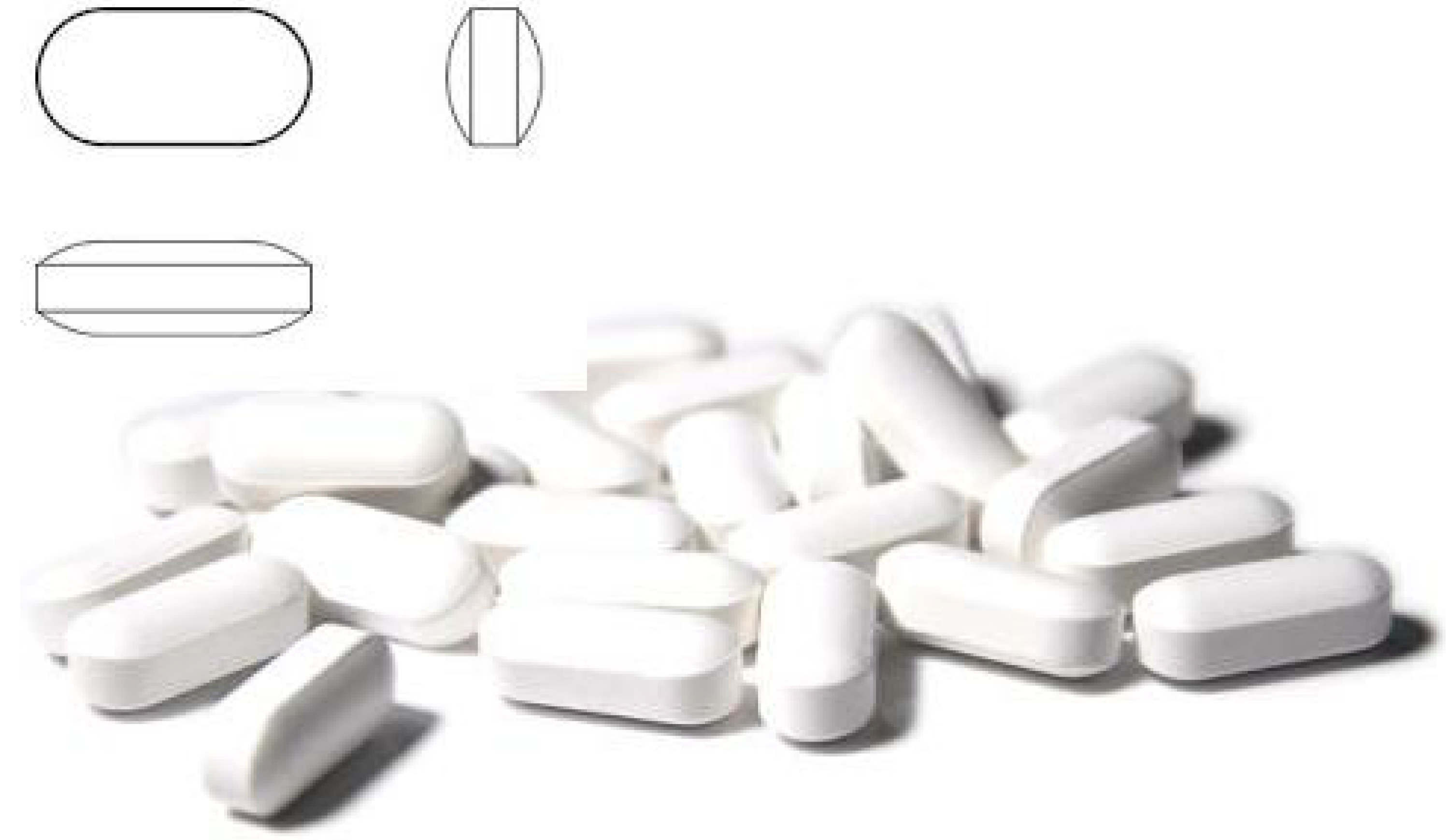
Figure 2.
Top: Vizualisation of simulated oblong tablets resting on a plane. Bottom: View from underneath; The corresponding footprint of the tablets. Squares belongs to upright standing tablets, thin stripes belongs to tablets landed on their round cap (green colored tablet for easy mapping of both views).
Figure 2.
Top: Vizualisation of simulated oblong tablets resting on a plane. Bottom: View from underneath; The corresponding footprint of the tablets. Squares belongs to upright standing tablets, thin stripes belongs to tablets landed on their round cap (green colored tablet for easy mapping of both views).
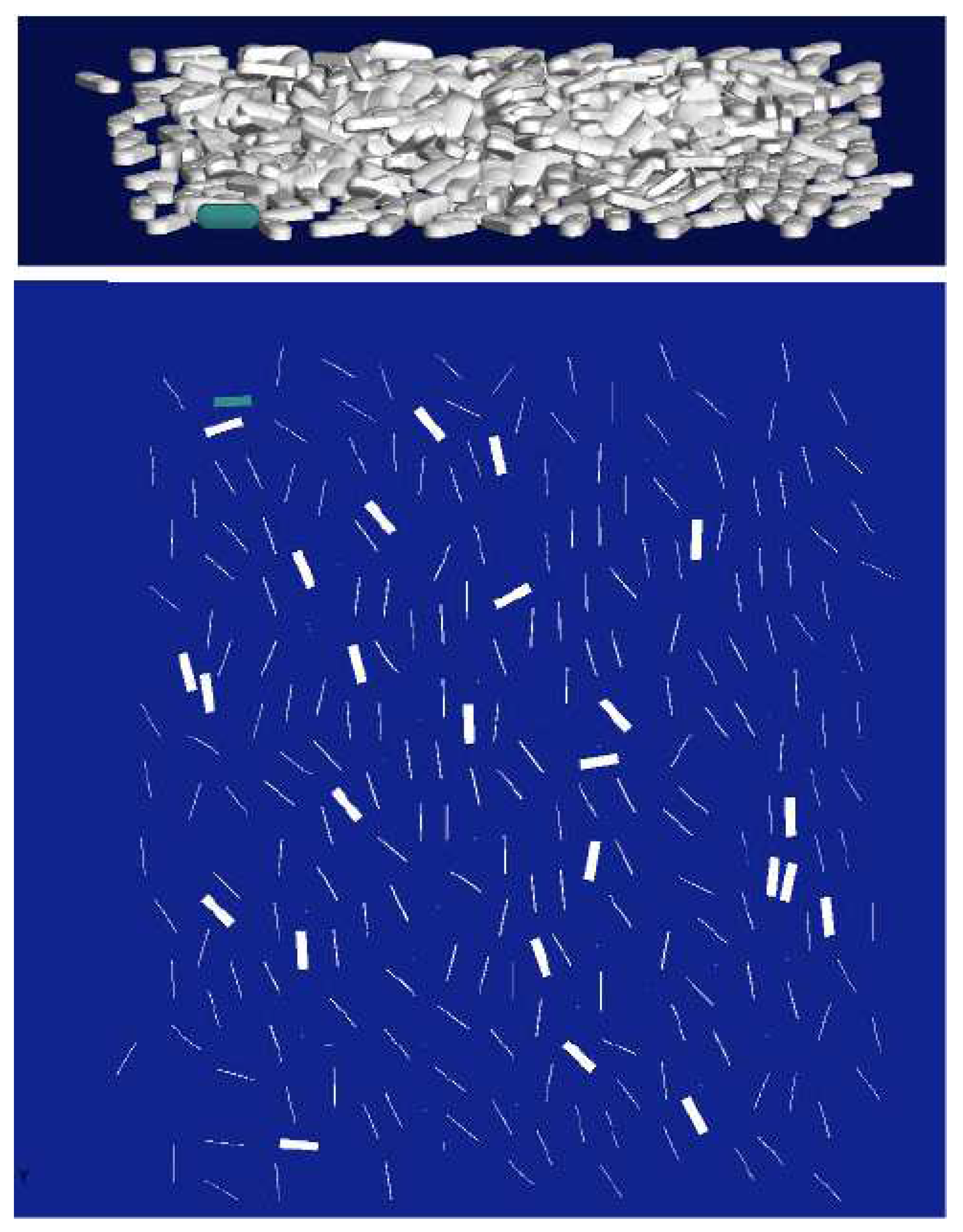
Figure 3.
Left: Song et al.: Representation of a bi-convex tablet using three convex surfaces. Right: Representation of an oblong tablet and its geometrical properties. is a single parameter which allows for total scaling of the shape.
Figure 3.
Left: Song et al.: Representation of a bi-convex tablet using three convex surfaces. Right: Representation of an oblong tablet and its geometrical properties. is a single parameter which allows for total scaling of the shape.
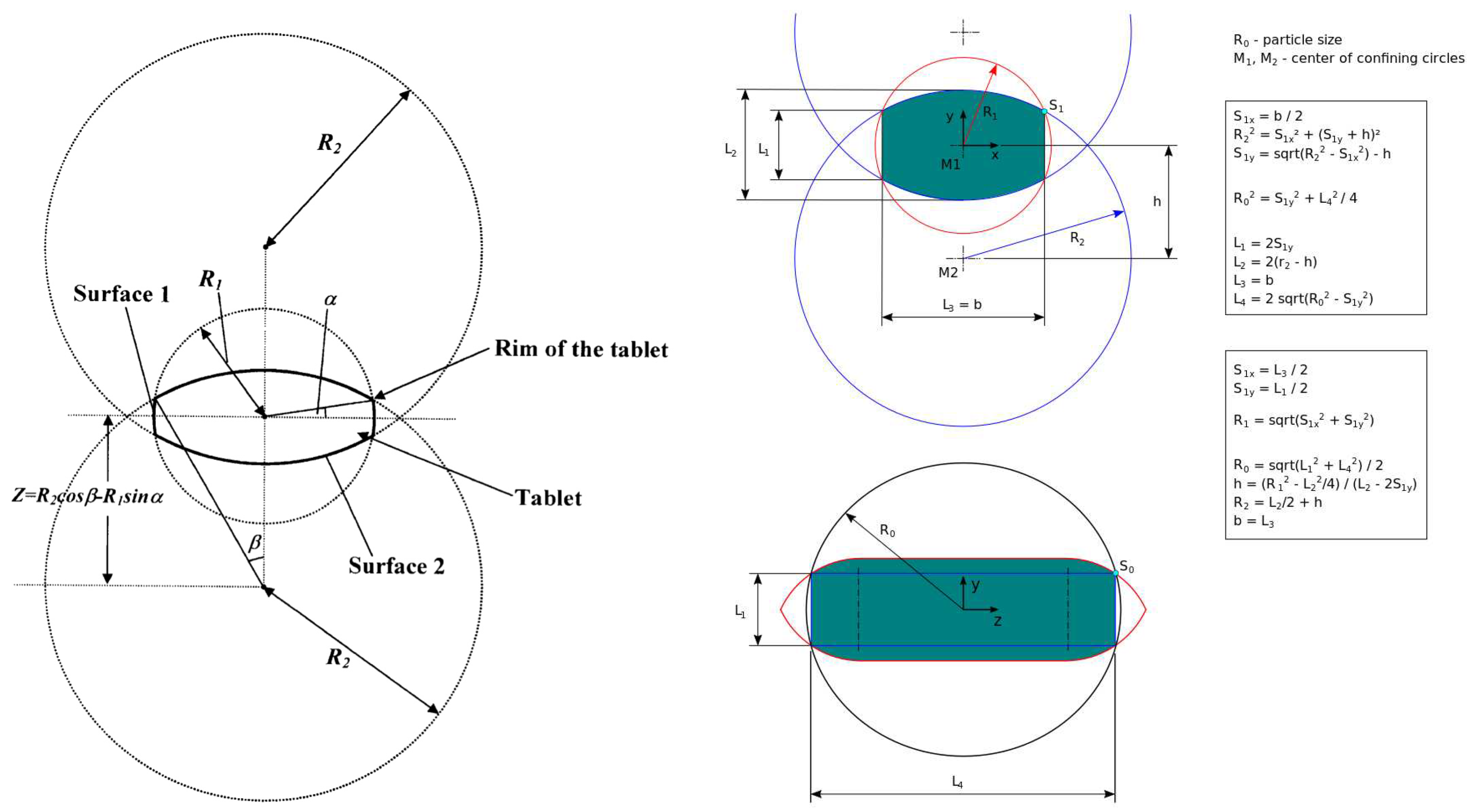
Figure 4.
a: The spherocylinder which forms a capsule is created by a sphere (green) moving along the axis. b: The resulting capsule shape. c: Schematic draw of contour shape creation. A bi-convex tablet is shifted along the axis of a sperocylinder (outer objet defined by the bounding sphere of the bi-convex tablet). The oblong tablet shape (transparent green) finally results by the contour of the moving bi-convex tablet and the terminal positions (arrows) at the lower end and upper end of the bodys axis. d: The resulting oblong tablet (score is a visual effect).
Figure 4.
a: The spherocylinder which forms a capsule is created by a sphere (green) moving along the axis. b: The resulting capsule shape. c: Schematic draw of contour shape creation. A bi-convex tablet is shifted along the axis of a sperocylinder (outer objet defined by the bounding sphere of the bi-convex tablet). The oblong tablet shape (transparent green) finally results by the contour of the moving bi-convex tablet and the terminal positions (arrows) at the lower end and upper end of the bodys axis. d: The resulting oblong tablet (score is a visual effect).
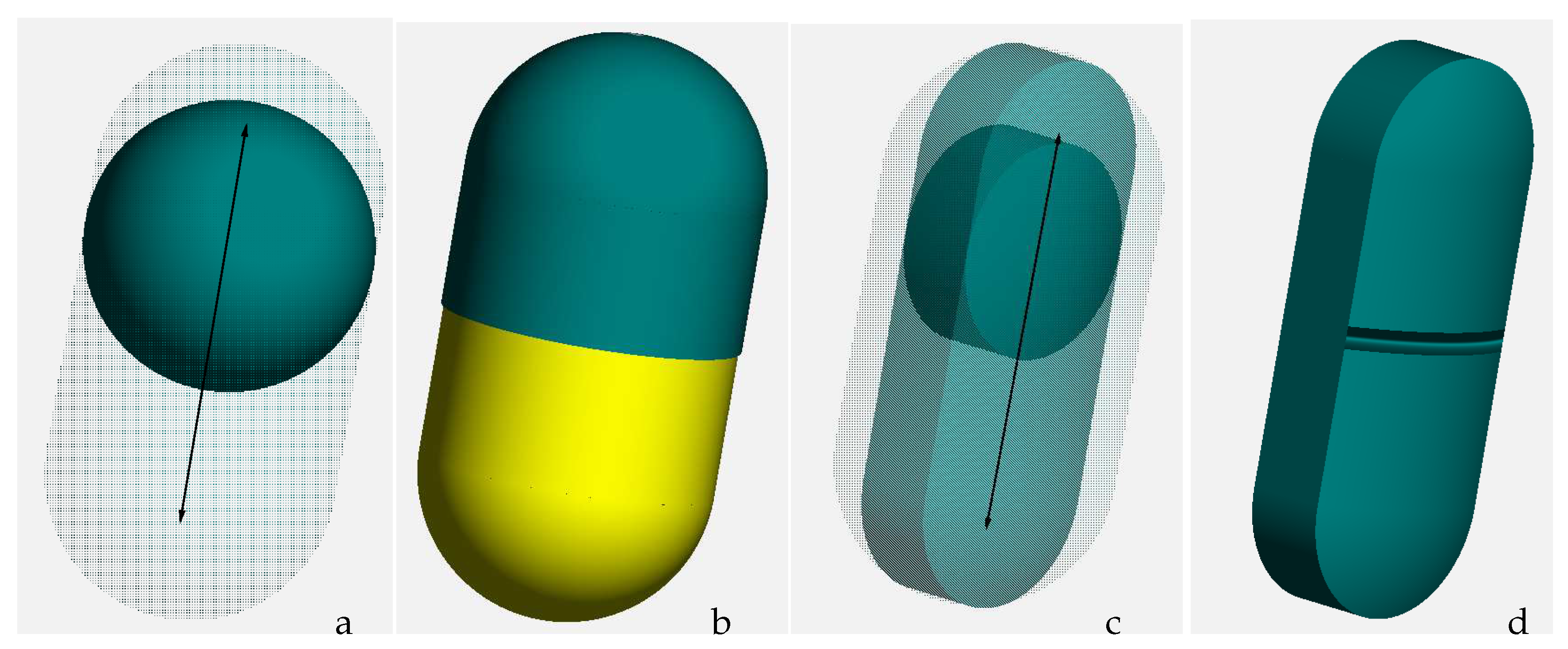
Figure 5.
True shape modeling properties of an oblong tablet. Left: Circumferending flat band (green), round caps on front side and back side and the sharp edge, called rim. Right: Band-band contact, two oblong tablets on top of each other and band-plane contact, tablets can rest on an STL surface.
Figure 5.
True shape modeling properties of an oblong tablet. Left: Circumferending flat band (green), round caps on front side and back side and the sharp edge, called rim. Right: Band-band contact, two oblong tablets on top of each other and band-plane contact, tablets can rest on an STL surface.
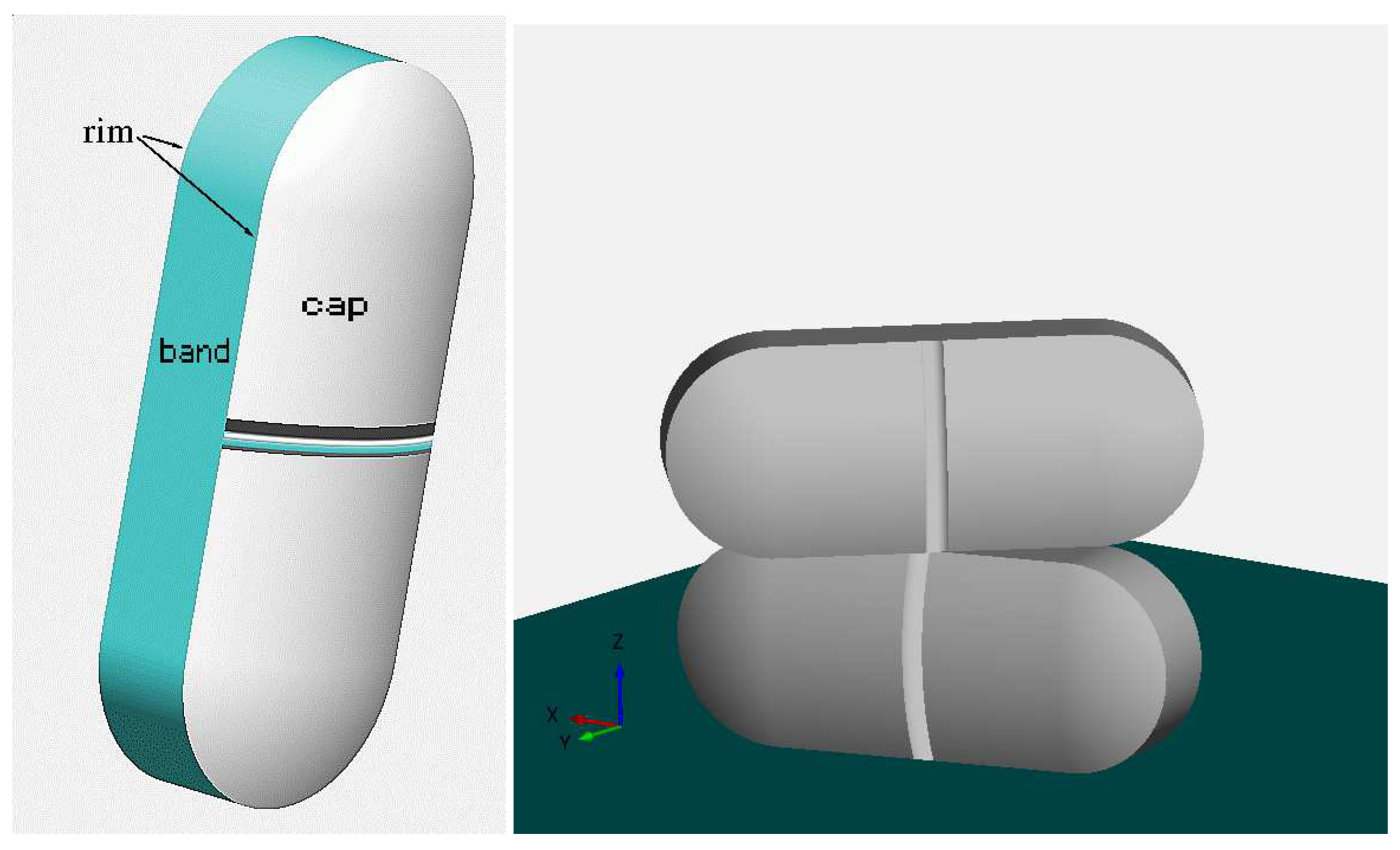
Figure 6.
View into a rotating drum. Only a few tablets are simulated for better visibility of the tablet climbing effect which occurs on rotating walls before tablets falling back onto the bed.
Figure 6.
View into a rotating drum. Only a few tablets are simulated for better visibility of the tablet climbing effect which occurs on rotating walls before tablets falling back onto the bed.
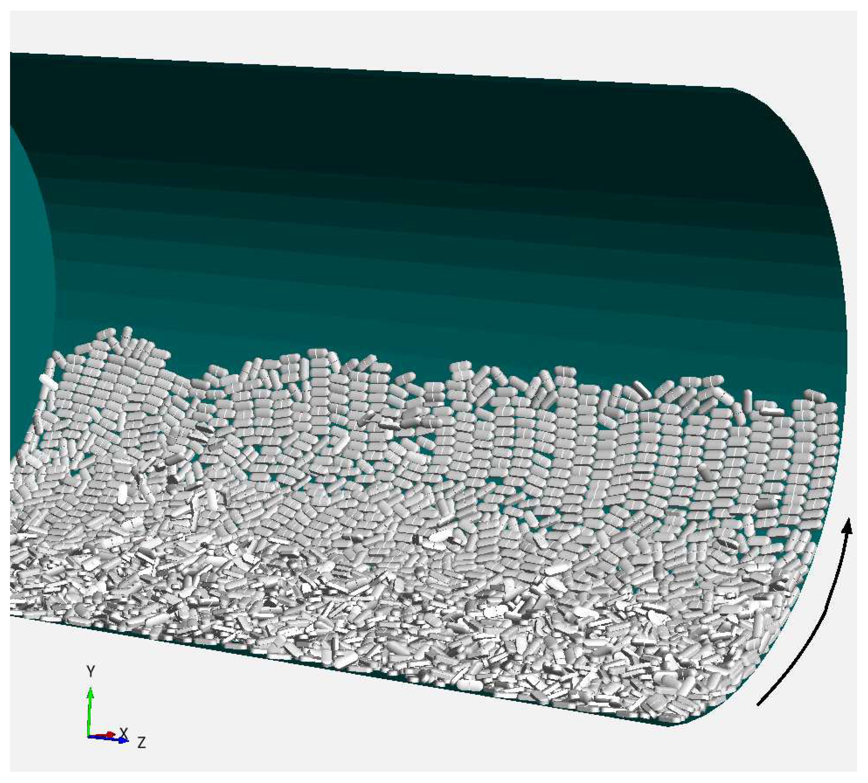
Figure 7.
Initial simulation setup. Talets filled at 40% fill level, drum resting, 0 rpm.
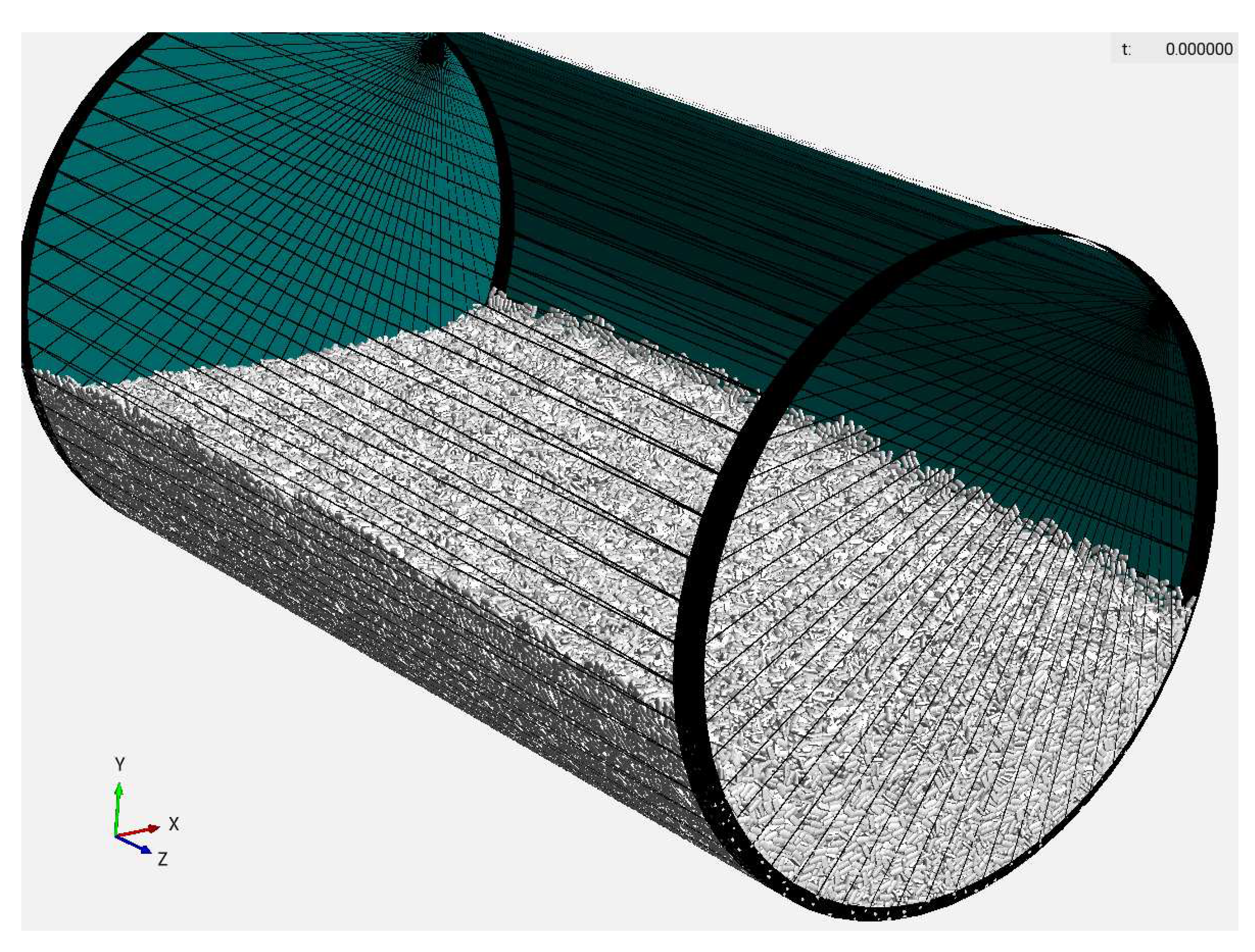
Figure 8.
Four different rpm cases, a=6 rpm, b=9 rpm, c=12 rpm, d=18 rpm. Side view, after 10 seconds mixing, using a smooth start from 0rpm to case target value within a period of one second.
Figure 8.
Four different rpm cases, a=6 rpm, b=9 rpm, c=12 rpm, d=18 rpm. Side view, after 10 seconds mixing, using a smooth start from 0rpm to case target value within a period of one second.
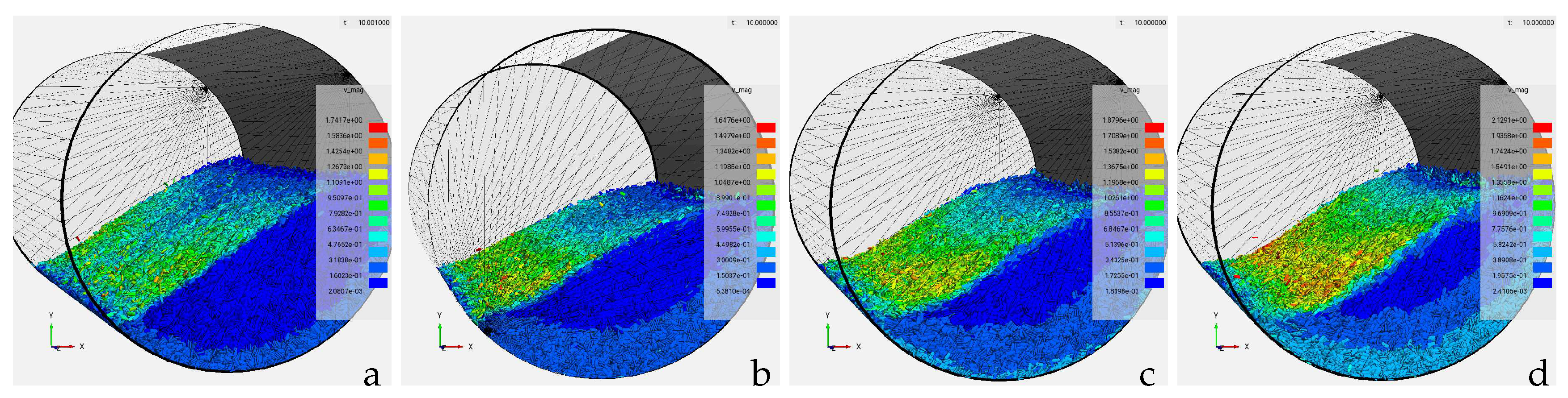
Figure 9.
Stacked bar chart histograms for 10s tablet mixing at 9 rpm (left) and 6 rpm (right).
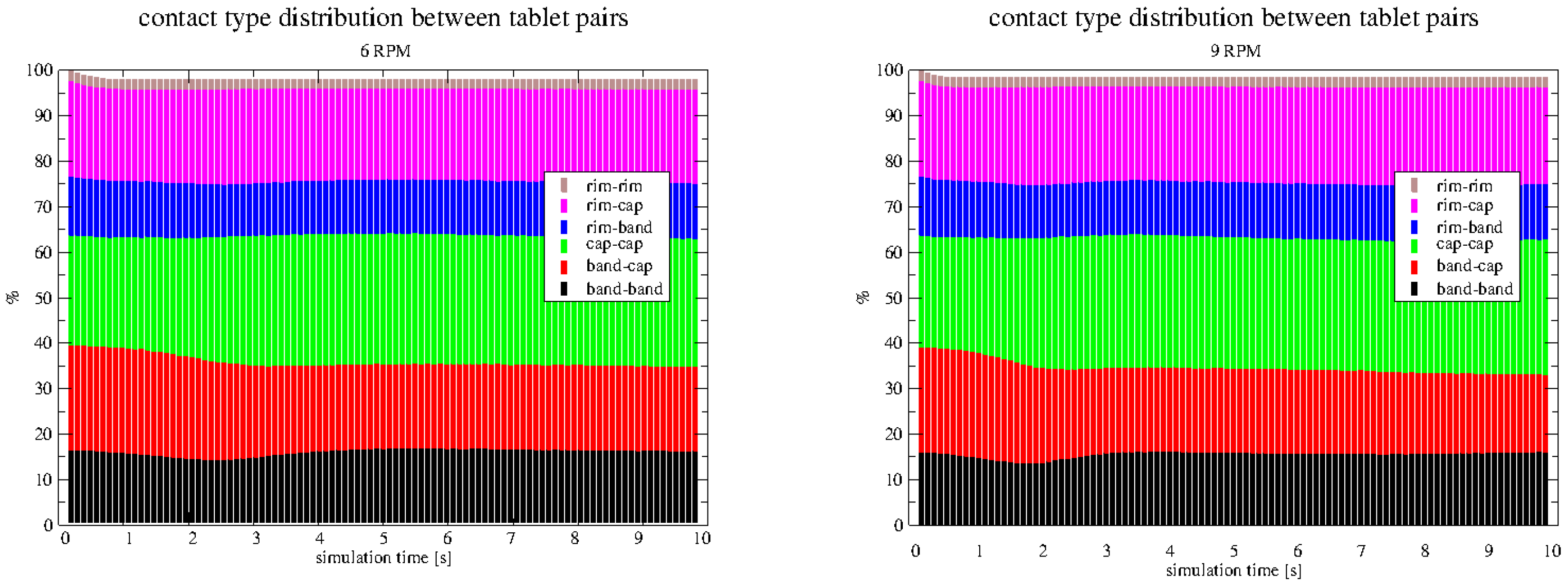
Figure 10.
Stacked bar chart histograms for 10s tablet mixing at 12 rpm (left) and 18 rpm (right).
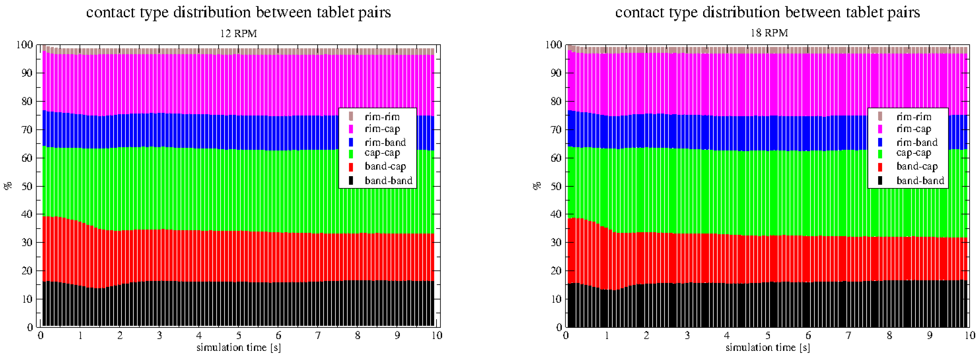
Figure 11.
Comparison after 10s operation time for all of the four cases a, b, c and d. With increasing rpm, a shift towards decreasing band-cap pairs take place. Whereas band-band pairs increase a bit. Other contact pairs ramain rather constant.
Figure 11.
Comparison after 10s operation time for all of the four cases a, b, c and d. With increasing rpm, a shift towards decreasing band-cap pairs take place. Whereas band-band pairs increase a bit. Other contact pairs ramain rather constant.
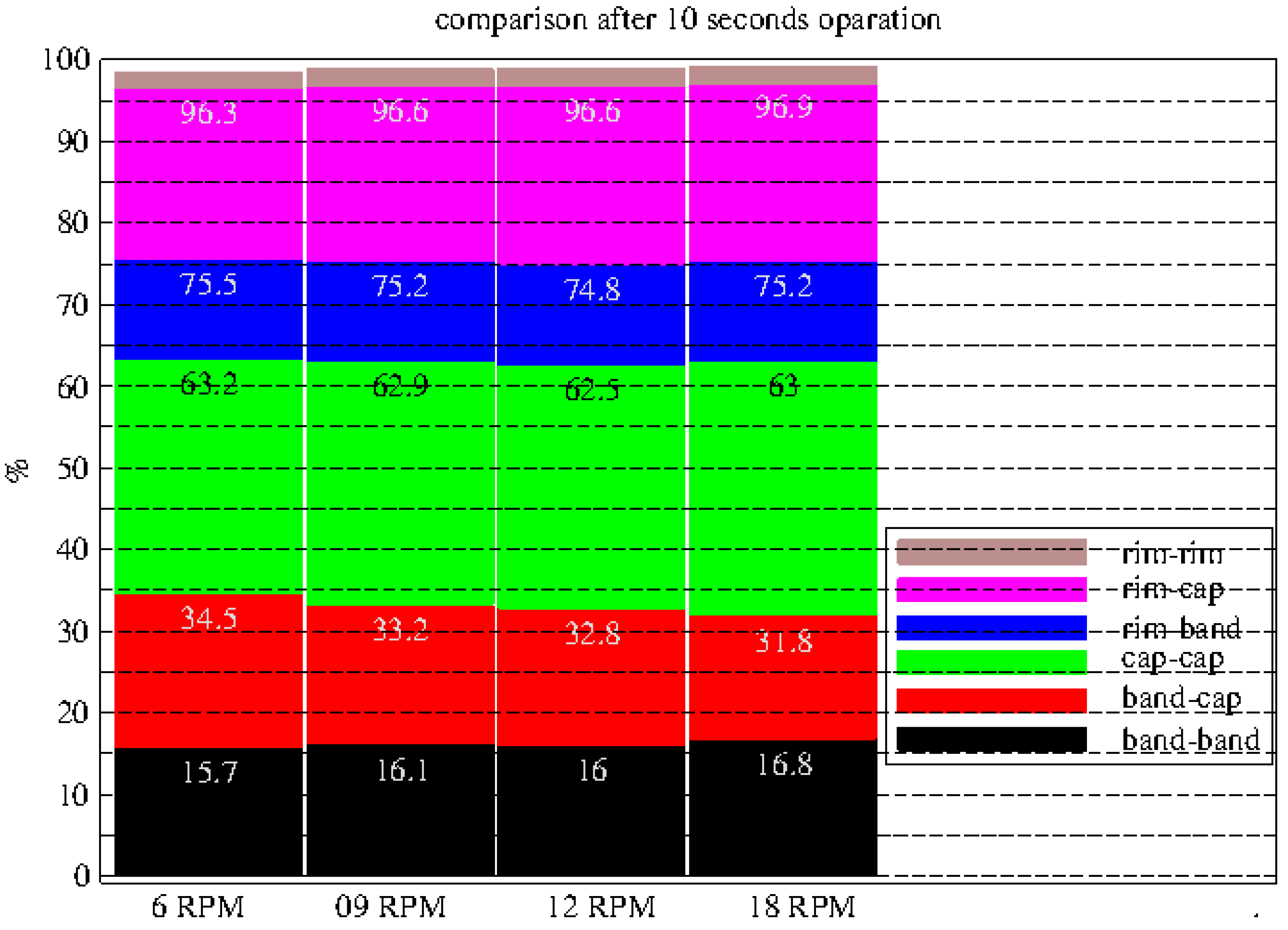
Figure 12.
Coating drum for simulation, look inside. Cylindrical main part with conical end for filling and discharging purposes (left). Smoothed baffles are placed in equal distance circumferending the interior wall.
Figure 12.
Coating drum for simulation, look inside. Cylindrical main part with conical end for filling and discharging purposes (left). Smoothed baffles are placed in equal distance circumferending the interior wall.
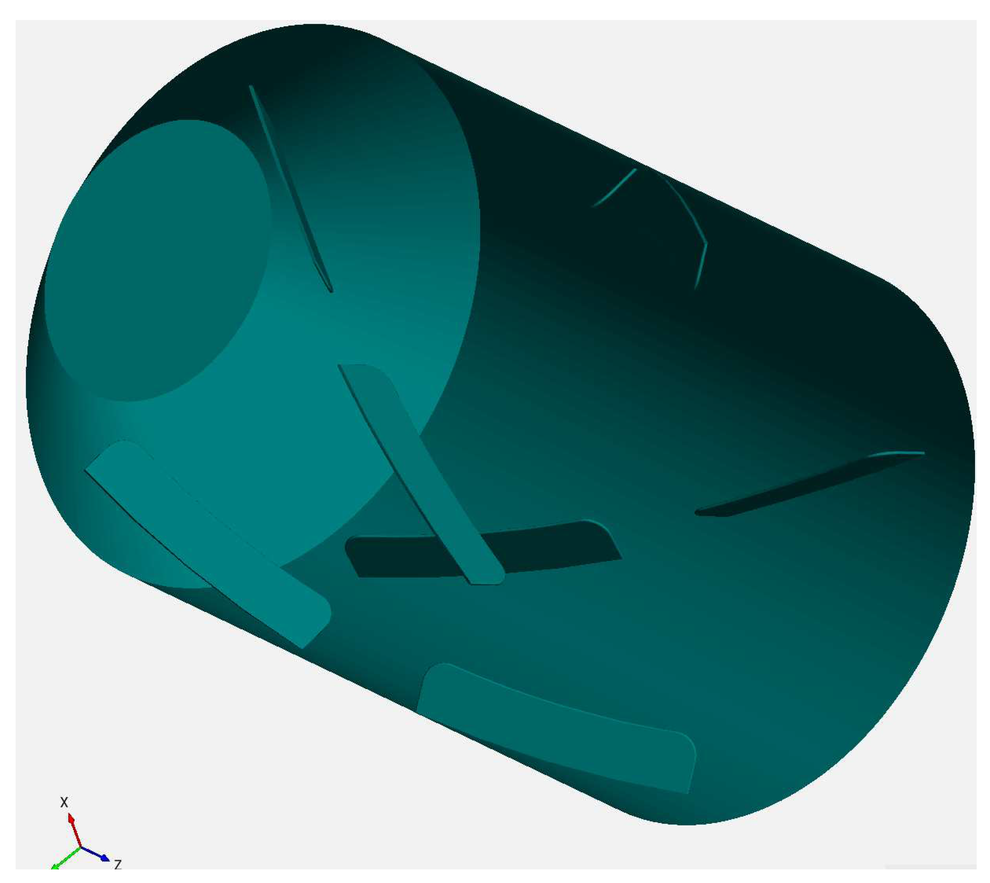
Figure 13.
View into the cutted drum: 370 kg batch. 2.54 million individual oblong tablets, ech of 114 mg mass. Drum speed is set to 6rpm.
Figure 13.
View into the cutted drum: 370 kg batch. 2.54 million individual oblong tablets, ech of 114 mg mass. Drum speed is set to 6rpm.
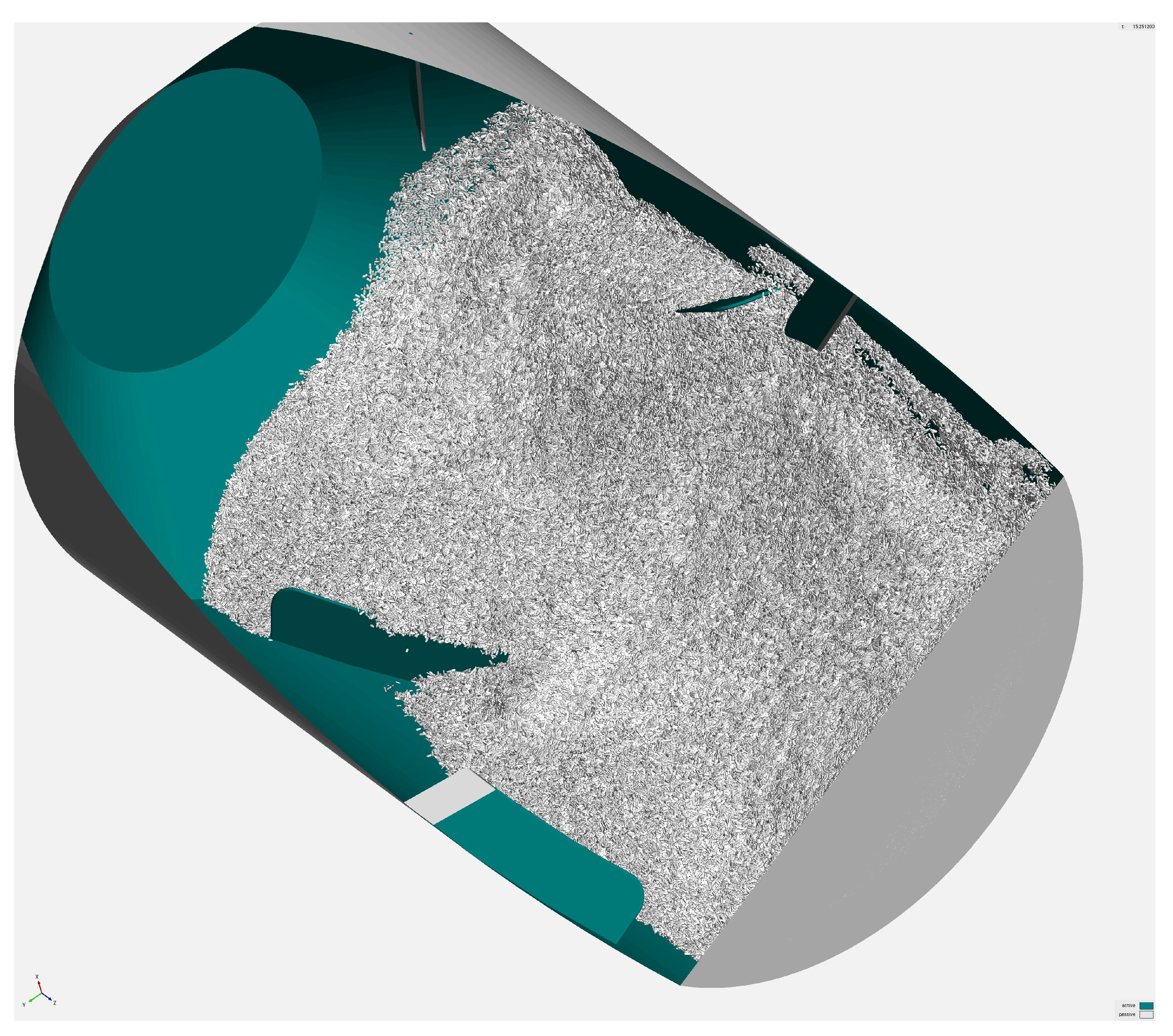
Figure 14.
370 kg batch contact pair statistics. After about 6s a steady state distribution of frequency of contact pairs has been reached.
Figure 14.
370 kg batch contact pair statistics. After about 6s a steady state distribution of frequency of contact pairs has been reached.
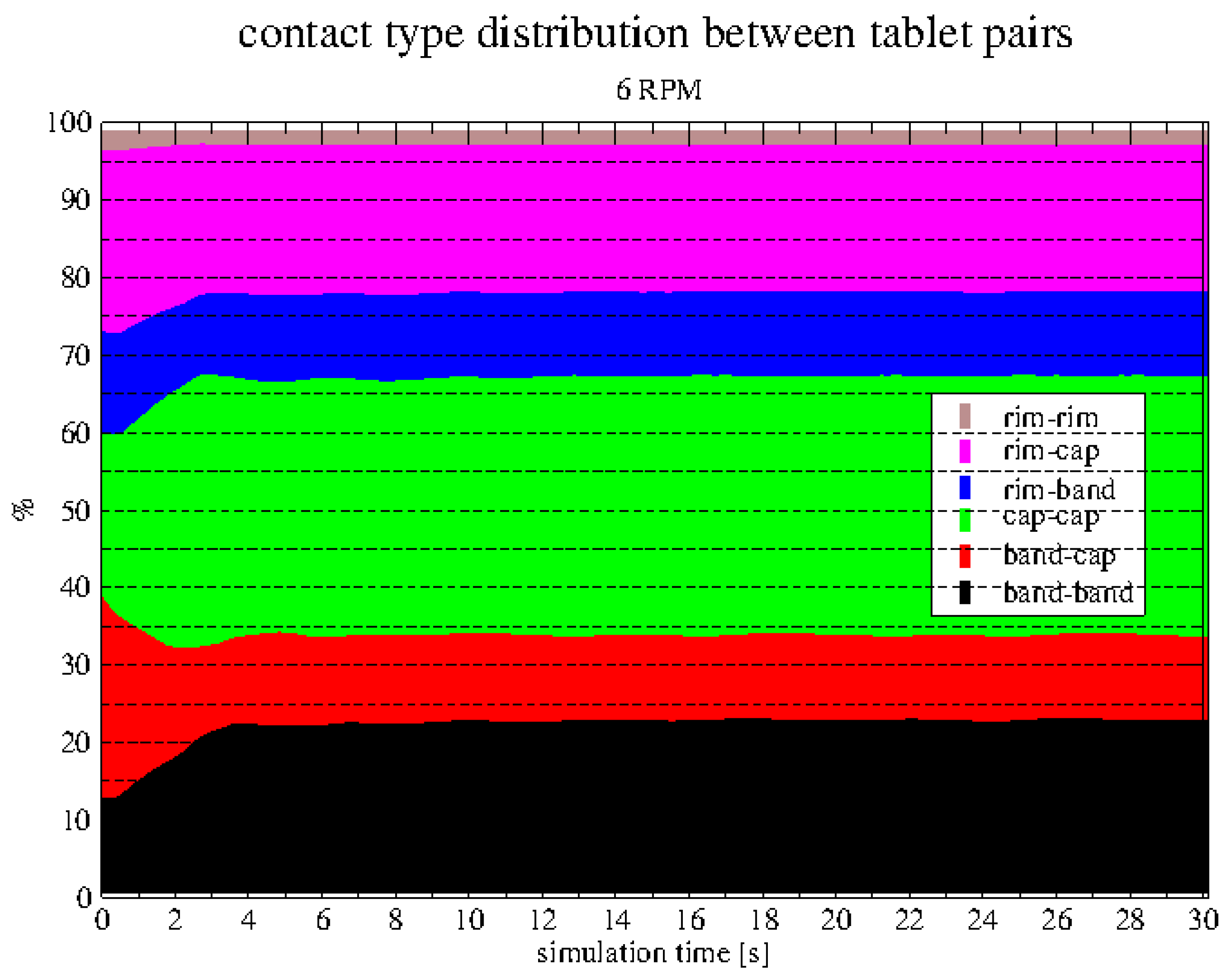
Figure 15.
2.54 million individual tablets result in over 20 million individual inter-tablet contacts. The diagram shows the evolution of number of contacts per tablet the so called coordination number. Black curve indicates the occuring contacts. Red curve shows the total contacts in the contact list which is build based on the number of the potential bounding sphere contacts.
Figure 15.
2.54 million individual tablets result in over 20 million individual inter-tablet contacts. The diagram shows the evolution of number of contacts per tablet the so called coordination number. Black curve indicates the occuring contacts. Red curve shows the total contacts in the contact list which is build based on the number of the potential bounding sphere contacts.
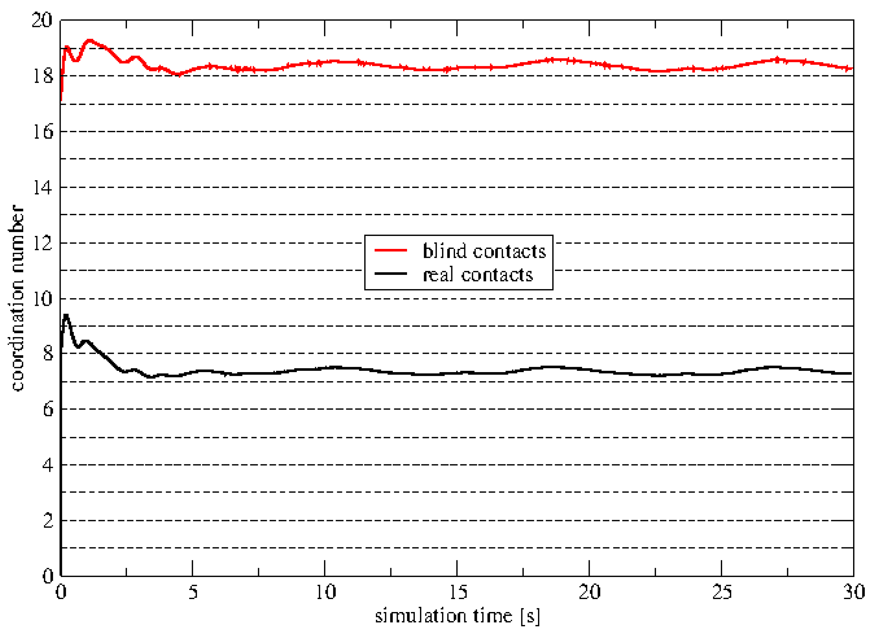
Figure 16.
At 15s simulation time: Empirical probability density function of contact normal force magnitudes between classified contact pairs. Higher forces acting on pairs with band-contribution (black, red, blue).
Figure 16.
At 15s simulation time: Empirical probability density function of contact normal force magnitudes between classified contact pairs. Higher forces acting on pairs with band-contribution (black, red, blue).
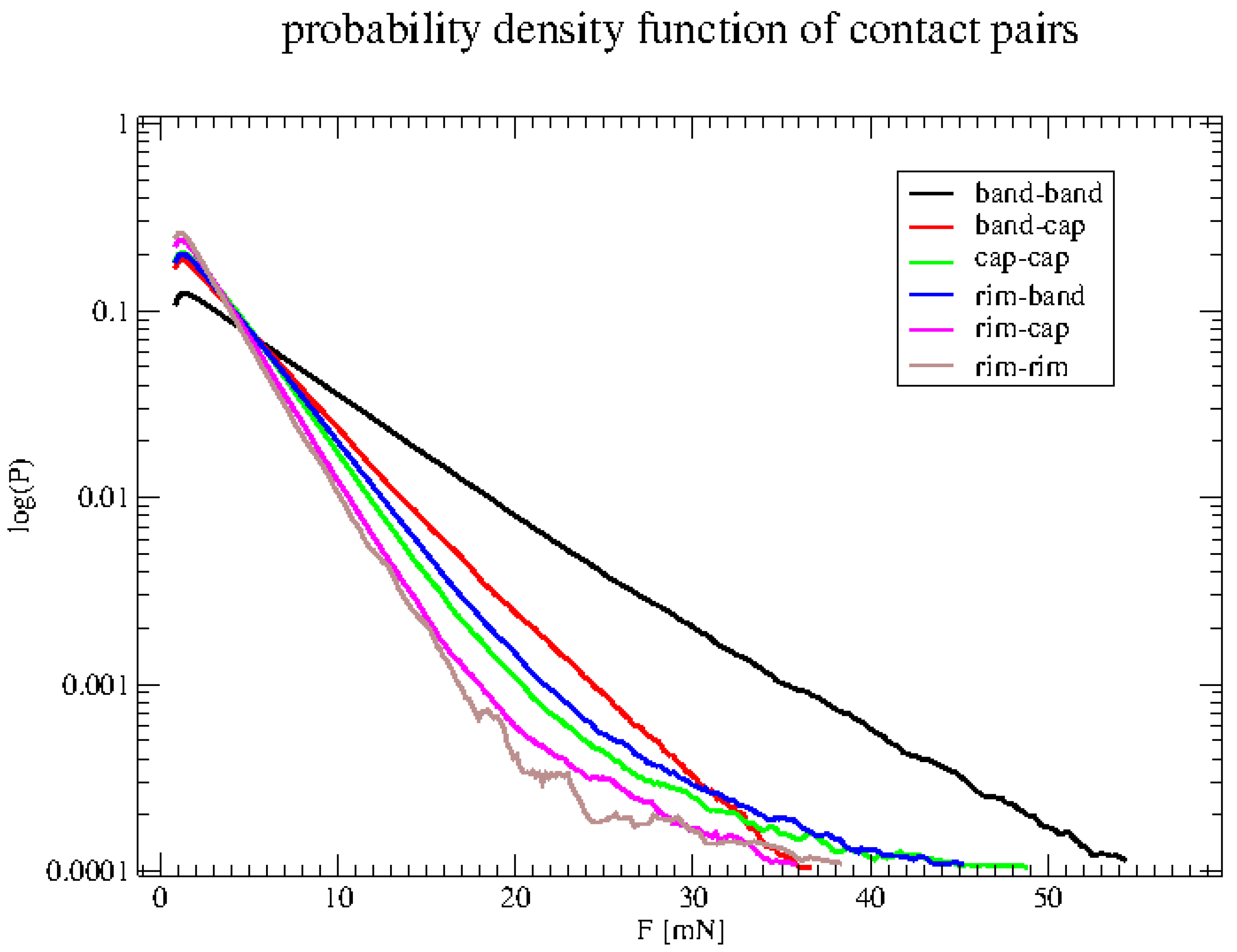
Table 1.
DEM simulation parameters 4x case studie.
| Parameter | Symbol | Value | Unit |
| Density | 1800 | ||
| Normal stiffness | |||
| Tangential stiffness | |||
| Restitution coefficent (normal) | e | 0.18 | |
| static friction (PP) | 0.6 | ||
| static friction (PW) | 0.6 |
Table 2.
Observations of histogram data after 10s mixingtime.
| band-band: | frequency increase slightly |
| band-cap: | frequency decrease |
| cap-cap: | frequency increase slightly |
| rim-band: | frequency remain rather constant |
| rim-cap: | frequency remain rather constant |
| rim-rim: | frequency remain constant |
Table 3.
DEM simulation parameters large batch.
| Parameter | Symbol | Value | Unit |
| Density | 1800 | ||
| Normal stiffness | |||
| Tangential stiffness | |||
| Restitution coefficent (normal) | e | 0.18 | - |
| static friction (PP) | 0.6 | - | |
| static friction (PW) | 0.85 | - | |
| time step | * | s |
* Simulation case ran with a Froude scaling approach, factor 10.0.
Table 4.
Maximum observed inter-tablet normal forces at different times mixingtime.
| contact type | force [mN] | |||
| 10s | 15s | 20s | 30s | |
| band-band: | 267.543 | 170.411 | 170.368 | 95.108 |
| band-cap: | 73.702 | 170.508 | 77.714 | 81.777 |
| cap-cap: | 121.394 | 127.872 | 125.214 | 130.2866 |
| rim-band: | 215.950 | 106.107 | 166.392 | 100.958 |
| rim-cap: | 67.680 | 75.741 | 60.780 | 75.500 |
| rim-rim: | 54.253 | 52.563 | 52.027 | 48.638 |
Disclaimer/Publisher’s Note: The statements, opinions and data contained in all publications are solely those of the individual author(s) and contributor(s) and not of MDPI and/or the editor(s). MDPI and/or the editor(s) disclaim responsibility for any injury to people or property resulting from any ideas, methods, instructions or products referred to in the content. |
© 2023 by the authors. Licensee MDPI, Basel, Switzerland. This article is an open access article distributed under the terms and conditions of the Creative Commons Attribution (CC BY) license (http://creativecommons.org/licenses/by/4.0/).
Copyright: This open access article is published under a Creative Commons CC BY 4.0 license, which permit the free download, distribution, and reuse, provided that the author and preprint are cited in any reuse.


