
Submitted:
26 October 2023
Posted:
26 October 2023
You are already at the latest version
Abstract
This paper presents three types of tensor Conjugate-Gradient methods for solving large-scale linear discrete ill-posed problems based on the t-product between third-order tensors. An automatical determination strategy of a suitable regularization parameter is proposed for the tensor conjugate gradient (tCG) method. A truncated version and a preprocessed verion of the tCG method are further presented. The discrepancy principle is employed to determine a suitable regularization parameter. Several numerical examples are given to show the effectiveness of the proposed tCG methods in image and video restoration.
Keywords:
linear discrete ill-posed problems
; tensor Conjugate-Gradient method
; t-product
; discrepancy principle
; Tikhonov regularization
1. Introduction
Tensors are high-dimensional arrays that have many applications in science and engineering, including in image, video and signal processing, computer vision, and network analysis [11,12,16,17,18,19,20,26]. A new t-product based on third-order tensors proposed by Kilmer et al [1,2]. When using high-dimensional data, t-product shows a greater potential value than matricization, see [2,6,11,12,21,22,24,25,27]. The t-product has been found to have special value in many application fields, including image deblurring problems [1,6,11,12], image and video compression [26], facial recognition problems [2], etc.
In this paper, we consider the solution of large minimization problems of the form
The Frobenius norm of singular tube of rapidly attenuates to zero with the increase of the index number. In particular, has ill-determined tubal rank. Many of its singular tubes are nonvanishing with tiny Frobenius norm of different orders of magnitude. Problems (1) with such a tensor is called the tensor discrete linear ill-posed problems. They arise from the restoration of color image and video, see e.g., [1,11,12]. Throughout this paper, the operation ∗ represents tensor t-product and denotes the tensor Frobenius norm or the spectral matrix norm.
We assume that the observed tensor is polluted by an error tensor , i.e.,
where is an unknown and unavailable error-free tensor related to . is determined by , where represents the explicit solution of problems (1) that is to be found. We assume that the upper bound of the Frobenius norm of is known, i.e,
Straightforward solution of (1) is usually meanless to get an approximation of because of the illposeness of and the error will be amplified severely. We use Tikhonov regularization to reduce this effect in this paper and replace (1) with penalty least-squares problems
where is a regularization parameter. We assume that
where denotes the null space of , is the identity tensor and is a lateral slice whose elements are all zero. The normal equation of minimization problem (4) is
then
is the unique solution of the Tikhonov minimization problem (4) under the assumption (5).
There are many techniques to determine the regularization parameter , such as the L-curve criterion, generalized cross validation (GCV), and the discrepancy principle. We refer to [4,5,8,9,10] for more details. In this paper, the discrepancy principle is extended to tensors based on t-product and is employed to determine a suitable in (4). The solution of (4) satisfies
where is usually a user-specified constant and is independent of in (3). When is smaller enough, and approaches 0, result in . For more details on the discrepancy principle, see e.g., [7].
In this paper, we also consider the expansion of minimization problem (1) of the form
where , .
There are many methods for solving large-scale discrete linear ill-posed problems (1). Recently, a tensor Golub- Kahan bidiagonalization method [11] and a GMRES method [12] were introduced for solving large-scale linear ill-posed problems (4). The randomized tensor singular value decomposition (rt-SVD) method in [3] was presented for computing super large data sets, and has prospects in image data compression and analysis. Ugwu and Reichel [23] proposed a new random tensor singular value decomposition (R-tSVD), which improves the truncated tensor singular value decomposition (T-tSVD) in [1]. Kilmer et al. [2] presented a tensor Conjugate-Gradient (t-CG) method for tensor linear systems corresponding to the least-squares problems. The regularization parameter in the t-CG method is user-specified. In this paper, we further discuss the automatical determinization of suitable regularization parameters of the tCG method by the discrepancy principle. The proposed method is called the tCG method with automatical determination of regularization parameters (auto-tCG). We also present a truncated auto-tCG method (auto-ttCG) to improve the auto-tCG method by reducing the computation. At last, a preprocessed version of the auto-ttCG method is proposed, which is abbreviated as auto-ttpCG.
The rest of this paper is organized as follows. Section 2 introduces some symbols and preliminary knowledge that will be used in the context. Section 3 presents the auto-tCG, auto-ttCG and auto-ttpCG methods for solving the minimization problems (4) and (9). Section 4 gives several examples on image and video restoration and Section 5 draws some conclusions.
2. Preliminaries
This section gives some notations and definitions, and briefly summarizes some results that will be used later. For a third-order tensor , Figure 1 shows the frontal slices , lateral slices and tube fibers . We abbreviate for simplication. An matrix is obtained by the operator , whereas the operator folds this matrix back to the tensor , i.e.,
Definition 1.
Let , then a block-circulant matrix of is denoted by , i.e.,
The following remarks will be used in Section 3.
Let be an n-by-n unitary discrete Fourier transform matrix, i.e,
where , then we get the tensor generated by using FFT along each tube of , i.e,
where ⊗ is the Kronecker product, is the conjugate transposition of and denetes the frontal slices of . Thus the t-product of and in (10) can be expressed by
and (10) is reformulated as
It is easy to calculate (12) in MATLAB.
For a non-zero tensor , we can decompose it in the form
where is a normalized tensor; see, e.g., [6] and is a tube scalar. Algorithm 1 summarizes the decomposition in (14).
| Algorithm 1 Normalization |
| Input: is a nonzero tensor |
| Output:, with , |
| fft(,[ ],3) |
| for do |
| ( is a vector) |
| if then |
| else |
| ; ; ; |
| end if |
| end for |
| ifft(,[ ],3); ifft(,[ ],3) |
Given a tensor , the singular value decomposition (tSVD) of is expressed as
where and are orthogonal under t-product,
is an upper triangular tensor with the singular tubes satisfying
The operators and [13] are expressed by
Figure 2 illustrates the transformation between a matrix and a tensor column by using and . Generally, the operators and are defined for a third-order tensor to make it squeezed or twisted. For a tensor with , means that all side slices of are squeezed and stacked as front slices of , the operator is the reverse operation of . Thus . We refer to Table 1 for more notations and definitions.
3. Tensor Conjugate-Gradient methods
This section first discusses the automatical determination of a suitable regularization parameter for the tensor conjugate gradient (tCG) method presented by Kilmer et al. in [13]. We abbreviate the improved method as auto-tCG. A truncated auto-tCG method is developed to improve the auto-tCG method and is abbreviated as auto-ttCG. A preprocessed version of the auto-ttCG method is presented, which is abbreviated as auto-ttpCG.
3.1. The auto-tCG Method
The tensor Conjugate-Gradient (t-CG) method is presented in [2] for the least-squares solution of the tensor linear systems . The regularization parameter in the t-CG method was not discussed and was user-specified. This subsection improves the t-CG method by employing the discrepancy principle to determine a suitable regularization parameter under the assumption (3) and uses it to solve the normal equation (6). We consider the polynomial function
where . We set , and obtain an optimal regularization parameter by continuously reducing the parameter. An effective method to deal with the general problems (9) is to regard it as p independent subproblems (4), i.e.,
where is the tensor column of the tensor and is polluted by the noise . represents unknown error-free tensor. Assume the noise tensor
can be used or the norm of can be estimated, i.e.,
Algorithm 2 summarizes the auto-tCG method for solving (9). The initial tensor of Algorithm 2 is set as zero tensor. The iteration is stopped when the Frobenius norm of the residual tensor
is small enough, where denotes the residual generated by the i-th iterative solution of the normal equation with of the j-th independent subproblem. Let be the initial tensor of the normal equation of . When with m iterations for the CG-process, the affine space is , where .
| Algorithm 2 The auto-tCG method for sloving (9). |
| Input:, , , , . |
| Output: Approximate solution of problem (9). |
| for do |
| . |
| while |
| , , e.g., |
| Normalize; . |
| , . |
| while do |
| . |
| . |
| . |
| . |
| . |
| end while |
| ( is the solution of the normal equation about of the j-th independent subproblem (4)). |
| end while |
| . |
| end for |
3.2. The truncated tensor Conjugate-Gradient method
Frommer and Maass in [15] proposed a good condition that can roughly judge some inappropriate value of . We introduce this condition to improve Algorithm 2 by excluding some unsuitable value of , and present a truncated tensor conjugate-gradient method for solving (9). We first give the following results.
Theorem 1.
Given , define a t-linear operator T: , i.e., with . Let be the exact solution of the normal equations
then for an arbitrary , we have
Proof.
For an arbitrary , set . Let the singular value decomposition of be , then
Suppose , then
Thus
Denote , and , then and . Thus we transform the tensor norm into the equivalent matrix norm. Let the singular value decomposition of be , where , and are orthogonal matrices with orthogonal columns and , respectively. Thus we have
Using the equation with the estimate
we have
Note that
It results from (19) and (20) that
Note that and , we have
Thus
Note that
then (23) and (22) result in
□
We will apply Theorem 1 to predict in advance whether the exact solution satisfies the discrepancy principle in Algorithm 2. We add the condition
in steps 9-16 of Algorithm 2. If the i-th iteration solution of the normal equation with is and its residual satisfies (24), then . This indicates that the exact solution of the normal equation with does not satisfy the discrepancy principle, so continue to solve next normal equation with . Therefore, we obtain a truncated tensor conjugate-gradient method of automatical determination of a suitable regularization parameter, which is abbreviated as auto-ttCG. Algorithm 3 summarizes the auto-ttCG method.
| Algorithm 3 The auto-ttCG method for sloving (9) |
| Input:, , , , , tol. |
| Output: Approximate solution of problem (9). |
| for do |
| while do |
| , , e.g.. |
| Normalize; . |
| , =10tol, . |
| while and do |
| . |
| . |
| , . |
| . |
| . |
| . |
| end while |
| . |
| end while |
| . |
| end for |
3.3. A preconditioned truncated tensor Conjugate-Gradient method
In this section, we consider the acceleration of Algorithm 3 by preconditioning. When the tensor is symmetric positive definite under the t-product structure, we can get its tensor approximate Cholesky decomposition (tChol) by Algorithm 4.
| Algorithm 4 Tensor Cholesky decomposition (tChol) |
|
In Algorithm 3, the coefficient tensor of the th normal equation
is symmetric and positive definite. We set and apply Algorithm 4 to obtain the decomposition of , where each frontal slice of is a fully sparse lower triangular matrix. After the normal equation (25) is preconditioned by , we solve the preconditioned normal equations
instead of equations (25) in Algorithm 3, where , , .
Applying Algorithm 3 to solve (26) instead of (25). Let and denote the solution of (25) and (26), respectively. Then we have
Let , , then we have
and
In addition, we have the iteration
and
together with
Taking the preprocessing procedure (27)-(35) into Algorithm 3, we obtain the improved auto-ttCG method, which is called the truncated tensor preconditioned conjugate-gradient method of automatical determination of a suitable regularization parameter, and is abbreviated as auto-ttpCG. Algorithm 5 summarizes the auto-ttpCG method. Numerical experiments in Section show Algorighm 5 converges faster than Algorithm 3.
| Algorithm 5 The auto-ttpCG method for sloving (9) |
| Input:, , , , , tol. |
| Output: Approximate solution of problem (9). |
| for do |
| while do |
| , . |
| ). |
| Normalize. |
| , . |
| , =10tol, . |
| while and do |
| . |
| . |
| , . |
| , |
| . |
| . |
| . |
| end while |
| . |
| end while |
| . |
| end for |
4. Numerical Examples
This section presents three examples to show the application of Algorithms 2, 3 and 5 on the restoration of image and video. All calculations are performed in MATLAB R2018a on computers with intel core i7 and 16GB ram.
Suppose is the k-th approximate solution to the minimization problem (9). The quality of the approximate solution is defined by the relative error
and the signal-to-noise ratio (SNR)
where denotes the uncontaminated data tensor and is the average gray-level of . The observed data in (9) is contaminated by a "noise" tensor , i.e., . is determined as follows. Let be the th transverse slice of , whose entries are scaled and normally distributed with a mean of zero, i.e.,
where the data of is generated according to N(0, 1).
Example 4.1 This example considers the restoration of the blurred and noised cameraman image with the size of . For the operator , its front slices are generated by using the MATLAB function blur, i.e.,
with , and . The condition numbers of are , while he condition numbers of the remaining slices are infinite. Let denote the original undaminated cameraman image. The operator converts into tensor column for storage. The noised tensor is generated by (36) with different noise level . The blurred and noisy images are generated by .
The auto-tCG, auto-ttCG and auto-ttpCG methods are used to solve the tensor discrete linear ill-posed problems (1). The discrepancy principle is employed to determine a suitable regularization parameter by using with and . We set in (8).
Figure 3 shows the convergence of relative errors verus (a) the iteration number k and (b) the CPU time for the auto-tCG, auto-ttCG and auto-ttpCG methods with the noise level corresponding in the Table 2. The iteration process is terminated when the discrepancy principle is satisfied. From Figure 3 (a), we can see that the auto-ttCG and auto-ttpCG methods do not need to solve the normal equation for all . This shows that the auto-ttCG and auto-ttpCG methods improve the auto-tCG method by the condition (24). Figure 3 (b) shows that the auto-ttpCG method converges fastest among three methods.
Table 2 lists the regularization parameter, the iteration number, the relative error, SNR and the CPU time of the optimal solution obtained by using the auto-tCG, auto-ttCG and auto-ttpCG methods with different noise levels . It can be seen from Table 2 that the auto-ttpCG method has the lowest relative error, highest SNR and the least CPU time for different noise level.
Figure 4 shows the reconstructed images obtained by using the auto-tCG, auto-ttCG and auto-ttpCG methods on the blurred and noised image with the noise level in Table 2. From Figure 4 we can see that the restored image by the auto-ttpCG method looks a bit better than others but the least CPU time.
Example 4.2 This example shows the restoration of a blurred color image by Algorithms 2, 3 and 5. The original image is stored as a tensor through the MATLAB function . We set and band=12, and get by
Then , and the condition number of other tensor slices of is infinite. The noise tensor is defined by (36). The blurred and noised tensor is derived by , which is shown in Figure 6 (a).
We set the color image to be divided into multiple lateral slices and independently process each slice through (1) by using the auto-tCG, auto-ttCG and auto-ttpCG methods. Figure 5 shows the convergence of relative errors verus (a) the iteration number k and (b) the CPU time for the auto-tCG, auto-ttCG and auto-ttpCG methods when dealing with the first tensor lateral slice of with . Similar results can be derived as that in Example 5.1 from Figure 5. We can see that the auto-ttCG and auto-ttpCG methods need less iterations than the auto-tCG method from Figure 5 (a) and the auto-ttpCG method converges fastest among all methods from Figure 5 (b).
Table 3 lists the relative error, SNR and the CPU time of the optimal solution obtained by using the auto-tCG, auto-ttCG and auto-ttpCG methods with different noise levels . The results are very similar to that in Table 2 for different noise level.

Table 3.
Example 4.2: Comparison of relative error, SNR, and CPU time between the auto-tCG, auto-ttCG and auto-ttpCG methods with different noise level .
Table 3.
Example 4.2: Comparison of relative error, SNR, and CPU time between the auto-tCG, auto-ttCG and auto-ttpCG methods with different noise level .
| Noise level | Method | Relative error | SNR | time (secs) |
| auto-tCG | 5.90e-02 | 14.62 | 314.73 | |
| auto-ttCG | 5.90e-02 | 14.62 | 262.81 | |
| auto-ttpCG | 5.43e-02 | 15.37 | 103.41 | |
| auto-tCG | 7.64e-02 | 12.37 | 117.48 | |
| auto-ttCG | 7.48e-02 | 12.55 | 62.01 | |
| auto-ttpCG | 7.01e-02 | 13.13 | 54.85 |
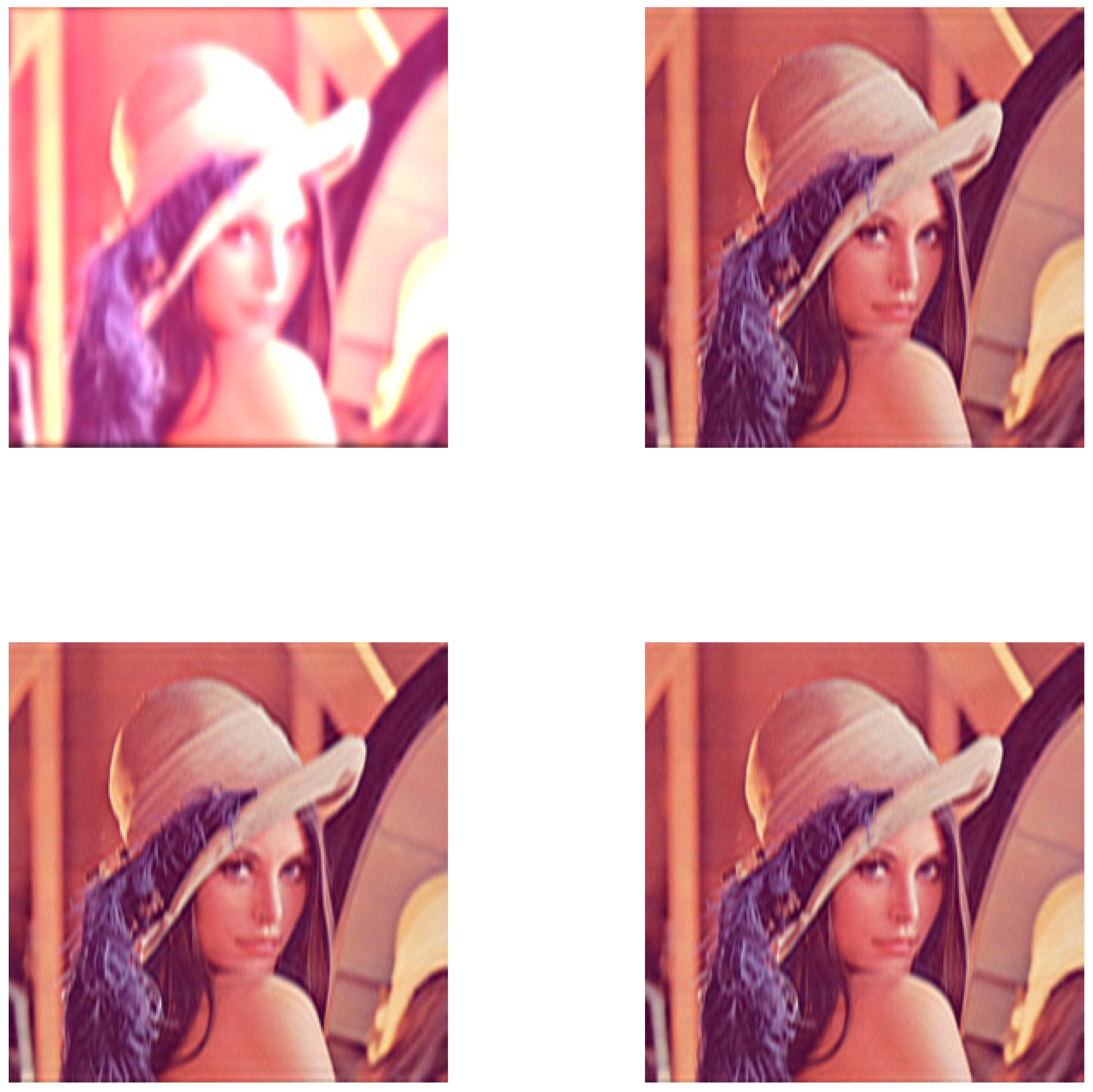
Figure 6 shows the recovered images by the auto-tCG, auto-ttCG and auto-ttpCG methods corresponding to the results with noise level . The results are very similar to that in Figure 6.
Figure 6.
Example 4.2: (a) The blurred and noised Lena image and reconstructed images by (b) the auto-tCG method, (c) the auto-ttCG and (d) the auto-ttpCG method according to the noise level in Table 3.
Figure 6.
Example 4.2: (a) The blurred and noised Lena image and reconstructed images by (b) the auto-tCG method, (c) the auto-ttCG and (d) the auto-ttpCG method according to the noise level in Table 3.
Example 4.3 (Video) We recover the first 10 consecutive frames of blurred and noised Rhinos video from MATLAB. Each frame has pixels. We store 10 pollution- and noise-free frames of the original video in the tensor . Let z be defined by (37) with , and . The coefficient tensor is defined as follows:
The condition number of the frontal slices of is , and the condition number of the remaining frontal sections of is infinite. The suitable regularization parameter is determined by using the discrepancy principle with . The blurred- and noised tensor is generated by with being defined by (36).
Figure 7 shows the convergence of relative errors verus the iteration number k and relative errors verus the CPU time for the auto-tCG, auto-ttCG and auto-ttpCG methods when the second frame of the video with is restored. Very similar results can be derived from Figure 7 to that in Example 5.1.
Table 4 displays the relative error, SNR and the CPU time of the optimal solution obtained by using the auto-tCG, auto-ttCG and auto-ttpCG methods for the second frame with different noise levels . We can see that the auto-ttpCG method has the largest SNR and the lowest CPU time for different noise level .
Figure 8 shows the original video, blurred and noised video, and the recovered video of the second frame of the video for the auto-tCG, auto-ttCG and the auto-ttpCG methods with noise level corresponding to the results in Table 4. The recovered frame by the auto-ttpCG method looks best among all recovered frames.
5. Conclusion
This paper presents three types of tensor Conjugate-Gradient methods for solving large-scale linear discrete ill-posed problems in tensor form. We first present an automatical determination strategy of a suitable regularization parameter for the tensor conjugate gradient (tCG) method. Furthermore, we develop a truncated version and a preprocessed verion of the tCG method. The proposed methods are used to different examples in image and video restoration.
Use of AI tools declaration
The authors declare they have not used Artificial Intelligence (AI) tools in the creation of this article.
Acknowledgements
The authors would like to thank the referees for their helpful and constructive comments. This research was supported in part by the Sichuan Science and Technology Program (grant 2022ZYD0008).
Conflict of interest
The authors declare no conflict of interest.
References
- Kilmer, M.E.; Martin, C.D. Factorization strategies for third order tensors. Linear Alg. Appl. 2011, 435, 641–658. [Google Scholar] [CrossRef]
- Hao, N.; Kilmer, M.E.; Braman, K.; Hoover, R.C. Facial recognition using tensor-tensor decompositions. SIAM J. Imaging Sci. 2013, 6, 437–463. [Google Scholar] [CrossRef]
- Zhang, J.; Saibaba, A. K.; Kilmer, M. E.; Aeron, S. A randomized tensor singular value decomposition based on the t-product. Numer. Linear Algebr. Appl. 2018, 25, e2179. [Google Scholar] [CrossRef]
- Fenu, C.; Reichel, L.; Rodriguez, G. GCV for tikhonov regularization via global Golub–Kahan decomposition. Numer. Linear Algebr. Appl. 2016, 25, 467–484. [Google Scholar] [CrossRef]
- Hansen, P.C. Rank-Deficient and Discrete Ill-Posed Problems; SIAM: Philadelphia, 1998. [Google Scholar]
- Kilmer, M. E.; Braman, K.; Hao, N.; Hoover, R. C. Third-order tensors as operators on matrices: A theoretical and computational framework with applications in imaging. SIAM J. Matrix Anal. Appl. 2013, 34, 148–172. [Google Scholar] [CrossRef]
- Engl, H. W.; Hanke, M.; Neubauer, A. Neubauer. In Regularization of Inverse Problems; Kluwer, Dordrecht, 1996. [Google Scholar]
- Kindermann, S. Convergence analysis of minimization-based noise level-free parameter choice rules for linear ill-posed problems. Electron. Trans. Numer. Anal. 2011, 38, 233–257. [Google Scholar]
- Kindermann, S.; Raik, K. A simplified L-curve method as error estimator. Electron.Trans. Numer. Anal. 2020, 53, 217–238. [Google Scholar] [CrossRef]
- Reichel, L.; Rodriguez, G. Old and new parameter choice rules for discrete ill-posed problems. Numer. Algorithms 2013, 63, 65–87. [Google Scholar] [CrossRef]
- Reichel, L.; Ugwu, U. O. The tensor Golub–Kahan–Tikhonov method applied to the solution of ill-posed problems with at-product structure. Numer. Linear Algebr. Appl. 2022, 29, e2412. [Google Scholar] [CrossRef]
- Ugwu, U. O.; Reichel, L. Tensor Arnoldi–Tikhonov and GMRES-Type Methods for Ill-Posed Problems with a t-Product Structure. J. Sci. Comput. 2022, 90, 1–39. [Google Scholar]
- Kilmer, M. E.; Braman, K.; Hao, N.; Hoover, R. C. Third-order tensors as operators on matrices: A theoretical and computational framework with applications in imaging. SIAM J. Matrix Anal. Appl. Appl. 2013, 34, 148–172. [Google Scholar] [CrossRef]
- Lund, K. The tensor t-function: A definition for functions of third-order tensors. Numer. Linear Algebr. Appl. 2020, 27, e2288. [Google Scholar] [CrossRef]
- Frommer, A.; Maass, P. Fast CG-based methods for Tikhonov–Phillips regularization. SIAM J. Sci. Comput. 1999, 20, 1831–1850. [Google Scholar] [CrossRef]
- Cichocki, A.; Mandic, D.; De Lathauwer, L.; Zhou, G.; Zhao, Q.; Caiafa, C.; Phan, H. A. Tensor decompositions for signal processing applications: From two-way to multiway component analysis. IEEE Signal Process. Mag. 2015, 32, 145–163. [Google Scholar] [CrossRef]
- Signoretto, M.; Tran Dinh, Q.; De Lathauwer, L.; Suykens, J. A. Learning with tensors: a framework based on convex optimization and spectral regularization. Mach. Learn., 2014, 94, 303-351. Mach. Learn. 2014, 94, 303–351. [Google Scholar] [CrossRef]
- Kilmer, M. E.; Horesh, L.; Avron, H.; Newman, E. Tensor-tensor algebra for optimal representation and compression of multiway data. Proceedings of the National Academy of Sciences. Proc. Natl. Acad. Sci. U. S. A. 2021, 118, e2015851118. [Google Scholar] [CrossRef] [PubMed]
- Beik, F. P. A.; Najafi–Kalyani, M.; Reichel, L. Iterative Tikhonov regularization of tensor equations based on the Arnoldi process and some of its generalizations. Appl. Numer. Math. 2020, 151, 425–447. [Google Scholar] [CrossRef]
- Bentbib, A. H.; Khouia, A.; Sadok, H. The LSQR method for solving tensor least-squares problems. Electron. Trans. Numer. Anal. 2022, 55, 92–111. [Google Scholar] [CrossRef]
- Bentbib, A. H.; El Hachimi, A.; Jbilou, K.; Ratnani, A. Fast multidimensional completion and principal component analysis methods via the cosine product. Calcolo 2022, 59, 26. [Google Scholar] [CrossRef]
- Khaleel, H. S.; Sagheer, S. V. M.; Baburaj, M.; George, S. N. Denoising of Rician corrupted 3D magnetic resonance images using tensor-SVD. Biomed. Signal Process. Control 2018, 44, 82–95. [Google Scholar] [CrossRef]
- Ugwu, U. O.; Reichel, L. Tensor regularization by truncated iteration: a comparison of some solution methods for large-scale linear discrete ill-posed problem with a t-product. arXiv 2021, arXiv:2110.02485. [Google Scholar]
- Zeng, C.; Ng, M. K. Decompositions of third-order tensors: HOSVD, T-SVD, and Beyond. Numer. Linear Algebr. Appl. 2020, 27, e2290. [Google Scholar] [CrossRef]
- El Hachimi, A.; Jbilou, K.; Ratnani, A.; Reichel, L. Spectral computation with third-order tensors using the t-product. Appl. Numer. Math. 2023, 193, 1–21. [Google Scholar] [CrossRef]
- Zheng, M. M.; Ni, G. Approximation strategy based on the T-product for third-order quaternion tensors with application to color video compression. Appl. Math. Lett. 2023, 140, 108587. [Google Scholar] [CrossRef]
- Yu, Q.; Zhang, X. (2023). T-product factorization based method for matrix and tensor completion problems. Comput. Optim. Appl. 2023, 84, 761–788. [Google Scholar] [CrossRef]
Figure 1.
(a) frontal slices , (b) lateral slices and (c) tube fibers
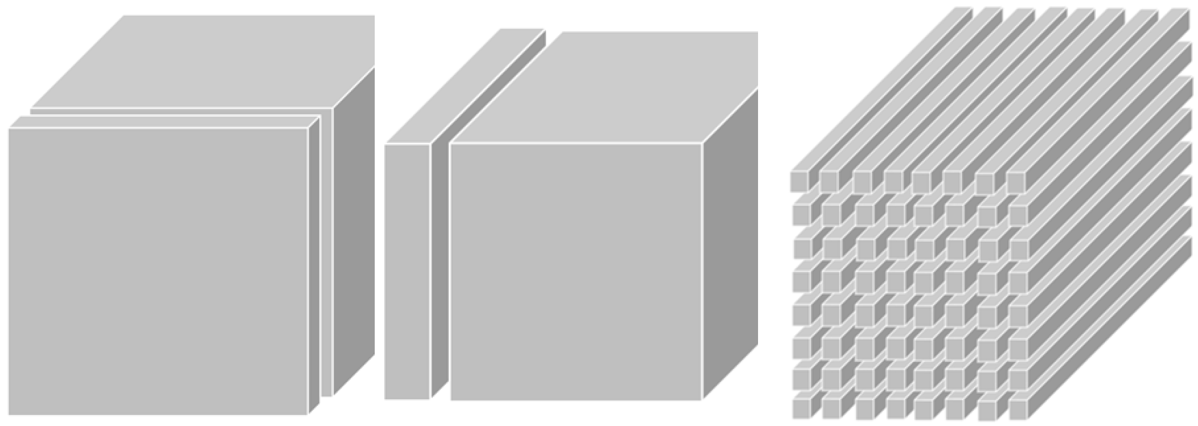
Figure 2.
twist-squeeze
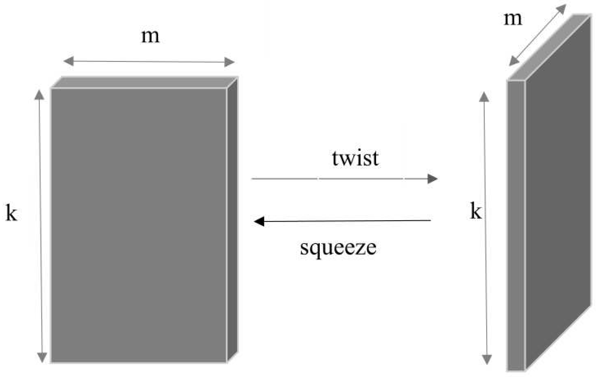
Figure 3.
Example 4.1: Comparison of convergence between (a) relative errors verus the iteration number k and (b) relative errors verus the CPU time for the auto-tCG, auto-ttCG and auto-ttpCG methods with the noise level .
Figure 3.
Example 4.1: Comparison of convergence between (a) relative errors verus the iteration number k and (b) relative errors verus the CPU time for the auto-tCG, auto-ttCG and auto-ttpCG methods with the noise level .
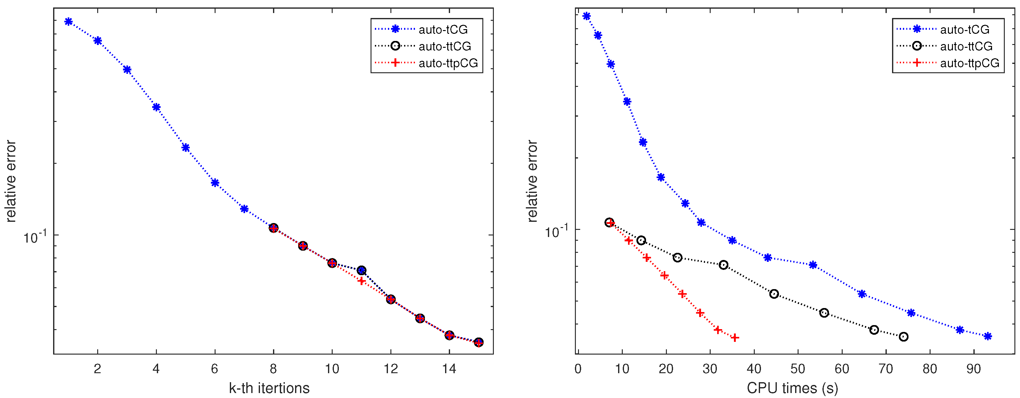
Figure 4.
Example 4.1: (a) The blurred and noised image and reconstructed images by (b) the auto-tCG method (SNR=22.36, CPU=109.87), (c) the auto-ttCG method (SNR=22.41, CPU=80.93) and (d) the auto-ttpCG method (SNR=22.48, CPU=33.98) according to the noise level in Table 2.
Figure 4.
Example 4.1: (a) The blurred and noised image and reconstructed images by (b) the auto-tCG method (SNR=22.36, CPU=109.87), (c) the auto-ttCG method (SNR=22.41, CPU=80.93) and (d) the auto-ttpCG method (SNR=22.48, CPU=33.98) according to the noise level in Table 2.
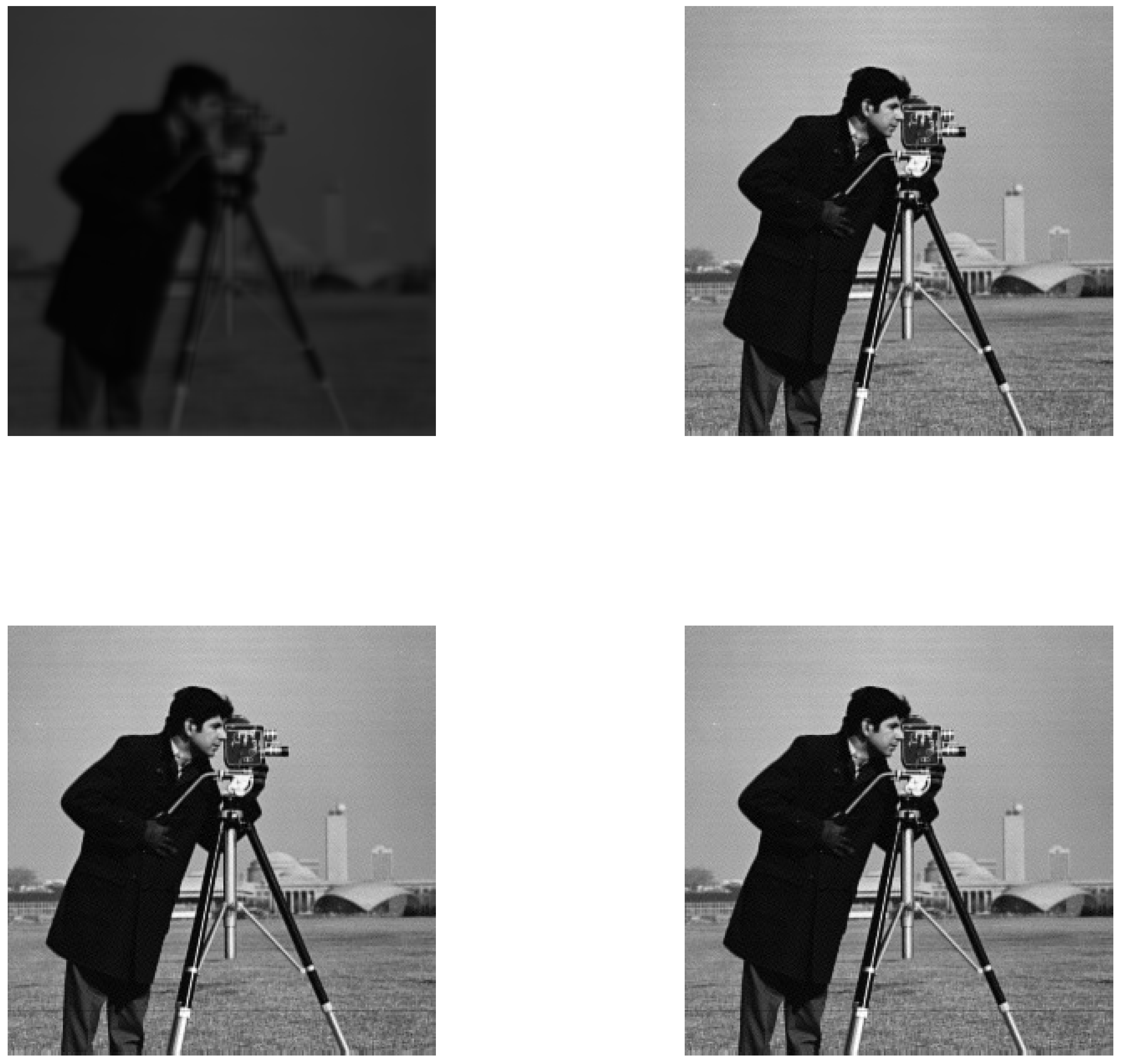
Figure 5.
Example 4.2: Comparison of convergence between (a) relative errors verus the iteration number k and (b) relative errors verus the CPU time for the auto-tCG, auto-ttCG and auto-ttpCG methods with the noise level .
Figure 5.
Example 4.2: Comparison of convergence between (a) relative errors verus the iteration number k and (b) relative errors verus the CPU time for the auto-tCG, auto-ttCG and auto-ttpCG methods with the noise level .
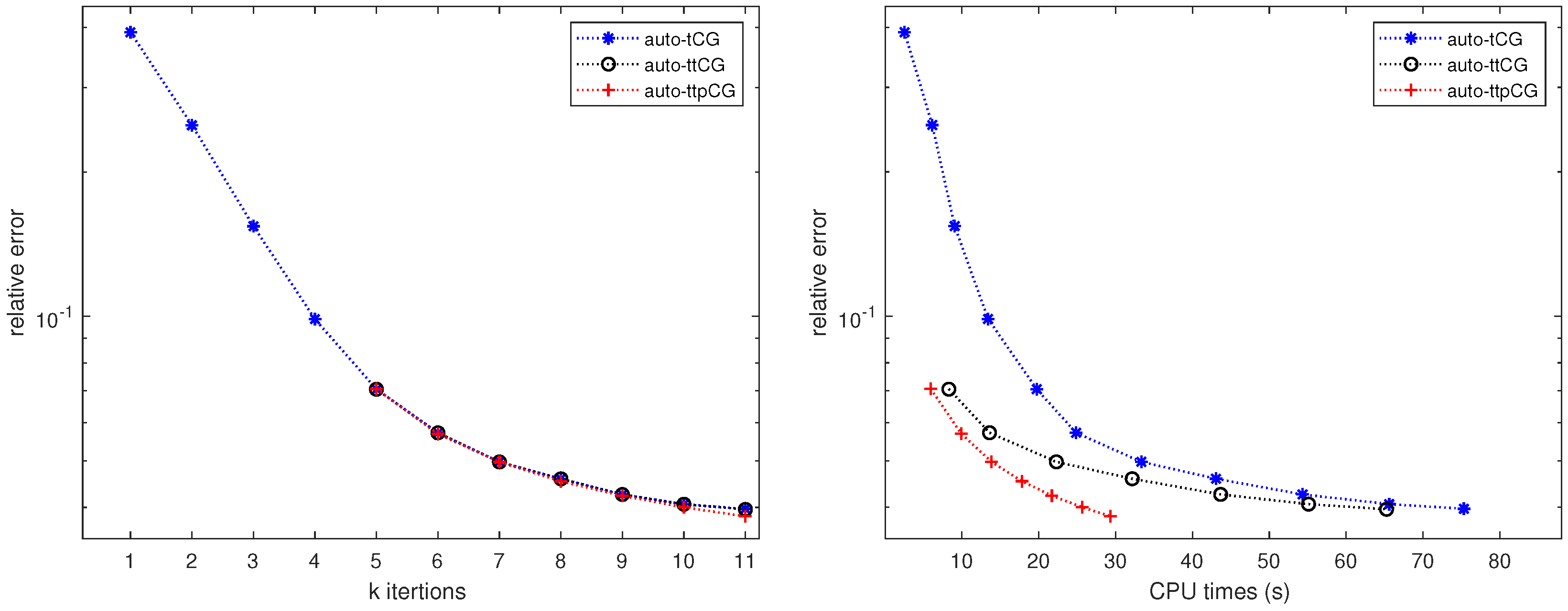
Figure 7.
Example 4.3: Comparison of convergence between (a) relative errors verus the iteration number k and (b) relative errors verus the CPU time for the auto-tCG, auto-ttCG and auto-ttpCG methods with the noise level .
Figure 7.
Example 4.3: Comparison of convergence between (a) relative errors verus the iteration number k and (b) relative errors verus the CPU time for the auto-tCG, auto-ttCG and auto-ttpCG methods with the noise level .
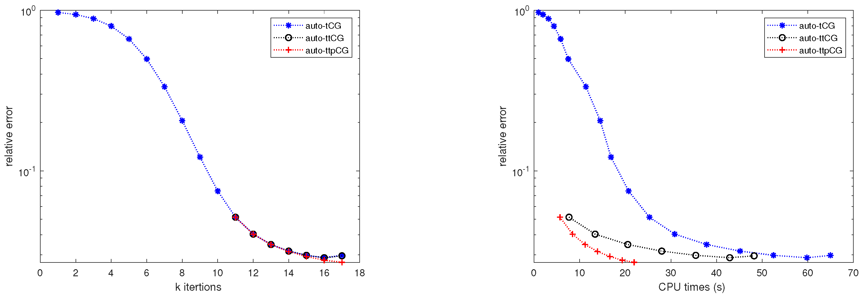
Figure 8.
Example 4.3: (a) Original image, (b) the blurred and noisy image and recovered images by (c) the auto-tCG method, (d) the auto-ttCG and (e) the auto-ttpCG method according to the noise level in Table 4.
Figure 8.
Example 4.3: (a) Original image, (b) the blurred and noisy image and recovered images by (c) the auto-tCG method, (d) the auto-ttCG and (e) the auto-ttpCG method according to the noise level in Table 4.
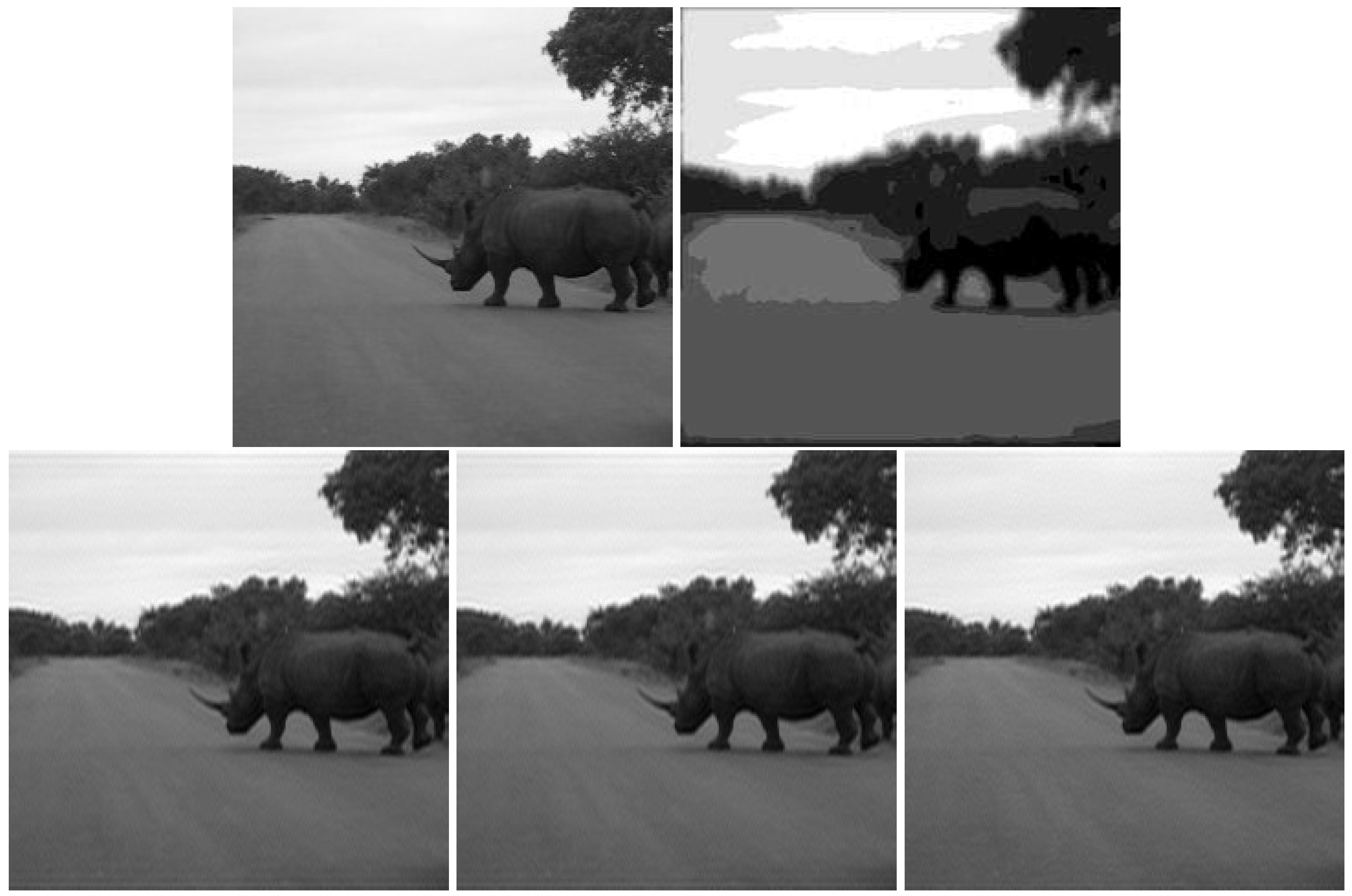
Table 1.
Description of notations
| Notation | Interpretation |
| transpose of tensors | |
| inverse of tensor, | |
| FFT of along the third mode | |
| the block column matrix of | |
| the block-circulant matrix | |
| identity tensor | |
| A | matrix |
| I | identity matrix |
| the Frobenius norm of tensors , i.e, | |
| ∗ | t-product |
| , | the jth tensor column of , jth lateral slice of |
| the jth frontal slice of tensor | |
| tube | |
Table 2.
Example 4.1: Comparison of relative error, SNR, and CPU time between the auto-tCG, auto-ttCG and auto-ttpCG methods with different noise level .
Table 2.
Example 4.1: Comparison of relative error, SNR, and CPU time between the auto-tCG, auto-ttCG and auto-ttpCG methods with different noise level .
| Noise level | Method | k | Relative error | SNR | CPU (secs) | |
| auto-tCG | 15 | 1.96e-05 | 3.54e-02 | 22.36 | 109.87 | |
| auto-ttCG | 15 | 1.96e-05 | 3.52e-02 | 22.41 | 80.93 | |
| auto-ttpCG | 15 | 1.96e-05 | 3.49e-02 | 22.48 | 33.98 | |
| auto-tCG | 11 | 3.14e-04 | 8.74e-02 | 14.51 | 81.94 | |
| auto-ttCG | 11 | 3.14e-04 | 8.64e-02 | 14.61 | 26.42 | |
| auto-ttpCG | 11 | 3.14e-04 | 8.54e-02 | 14.72 | 18.50 |
Table 4.
Example 4.3: Comparison of relative error, SNR, and CPU time between the auto-tCG, auto-ttCG and auto-ttpCG methods with different noise level .
Table 4.
Example 4.3: Comparison of relative error, SNR, and CPU time between the auto-tCG, auto-ttCG and auto-ttpCG methods with different noise level .
| Noise level | Method | Relative error | SNR | time (secs) |
| auto-tCG | 2.94e-02 | 23.17 | 697.78 | |
| auto-ttCG | 2.92e-02 | 23.23 | 487.35 | |
| auto-ttpCG | 2.66e-02 | 24.05 | 214.16 | |
| auto-tCG | 5.24e-02 | 18.15 | 480.75 | |
| auto-ttCG | 5.10e-02 | 18.38 | 281.54 | |
| auto-ttpCG | 4.74e-02 | 19.02 | 156.44 |
Disclaimer/Publisher’s Note: The statements, opinions and data contained in all publications are solely those of the individual author(s) and contributor(s) and not of MDPI and/or the editor(s). MDPI and/or the editor(s) disclaim responsibility for any injury to people or property resulting from any ideas, methods, instructions or products referred to in the content. |
© 2023 by the authors. Licensee MDPI, Basel, Switzerland. This article is an open access article distributed under the terms and conditions of the Creative Commons Attribution (CC BY) license (http://creativecommons.org/licenses/by/4.0/).
Copyright: This open access article is published under a Creative Commons CC BY 4.0 license, which permit the free download, distribution, and reuse, provided that the author and preprint are cited in any reuse.


