Submitted:
24 October 2023
Posted:
25 October 2023
You are already at the latest version
Abstract
Agricultural drainage canals that connect upstream fish spawning areas to downstream rivers and lakes serve as crucial habitats for migrating fish. However, disconnections, such as drops and chutes, have been constructed in these canals due to agricultural modernization and flood control measures, hindering the movement of fish with limited swimming abilities. Portable fishways offer a promising solution to reconnect water bodies in agricultural canals, as they can be easily removed during high water discharges to avoid impeding the canals' drainage function. In addition to experimental assessments of fishway functionality, employing a hydrodynamic model to explore effective placement strategies for portable fishways is essential to maximize their effectiveness. This study presents a method to determine the best horizontal location of a portable fishway in an agricultural drainage canal using two-dimensional hydrodynamic simulations within the specified cases. The applicability of this method is demonstrated by addressing the positioning challenge of a portable fishway on a chute in an agricultural drainage canal in Japan. Results indicate that the proposed method allows for the selection of a suitable location, considering preferable hydraulic conditions both within the portable fishway and around its entrance.
Keywords:
portable fishway
; hydraulic environment
; agricultural drainage canal
; chute
; effective positioning
; two-dimensional hydrodynamic simulation
1. Introduction
Agricultural drainage canals play a vital role in providing important habitats for migrating fish by linking areas where they spawn in the upper reaches to downstream rivers and lakes. Regrettably, these canals have experienced disruptions like drops and chutes due to advancements in agriculture and flood control efforts. These disruptions have created obstacles for fish that are unable to swim against fast currents. To address this issue, portable fishways offer a promising solution. They can be conveniently installed in these canals and easily removed during periods of high water flow to ensure that the canals can perform their drainage function.
Many studies on installing fishways have been conducted in the world. However, most of the previous studies employed a comparatively large-scale fishway intended for long-term use made of concrete, which can be called a “permanent fishway.” A permanent fishway requires considerable labor, capital costs, and time for installation. Therefore, it is difficult to conserve migratory aquatic organisms in waterbodies using only permanent fishways. In contrast, a portable fishway can be manufactured at a low cost and does not require specialized knowledge for installation. Takahashi et al. (2021) developed a portable fishway system that can be used in agricultural canals, and demonstrated its effectiveness through laboratory and field experiments [1]. A portable fishway can be attached and detached by farmers and local residents to help fish pass through a disconnected area caused by a chute and a drop in an agricultural canal during a particular season or day.
Fishways can be classified into four types: vertical-slot, pool-weir, Denil, and culvert fishways [2]. Experimental and numerical investigations of the flow in permanent fishways were conducted. For example, An et al. (2016) simulated the three-dimensional flow to facilitate the design of a vertical-slot fishway [3]. Gao et al. (2016) developed a numerical model to simulate the trajectories of a virtual fish through a vertical-slot fishway by computing a turbulent flow field [4]. Zhong et al. (2021) investigated the hydraulic performance of a semi-frustum weir in a pool-weir fishway using both experimental and numerical methods [2]. Amaral et al. (2019) assessed several types of retrofitted ramped weirs to improve the passage of potamodromous fish using experiments and numerical simulations of flow [5]. Chorda et al. (2019) conducted numerical modeling of the free surface flow across a steeply sloped ramp covered with staggered surface emergent cylinders [6].
Very few studies have been conducted on numerical simulation of flow in a portable fishway. Sudo (2020) applied a portable fishway on a chute (steep slope) of an agricultural drainage canal in Ibaraki, Japan and conducted a demonstration test to determine whether it promoted the ascent of small aquatic animals [7]. The results showed that the flow velocity in the fishway decreased to less than half of the flow velocity in the chute of the drainage canal, and that medaka (Oryzias latipes) and Yoshinobori goby (orange type; Rhinogobius sp. OR) [8] went up the fishway. Yoshinari et al. (2021) [9] simulated the two-dimensional flow in the portable fishway of Sudo (2020) [7] and identified regions of high current velocity and low water depth under several longitudinal gradients of fishway and discharge conditions. However, the hydraulic influence of the portable fishway downstream in the canal and its effective location for fish migration have not been investigated.
Experimental assessments of functionality of a portable fishway are insufficient for its effective use because several key issues remain unexamined. One of the problems is the positioning of the portable fishway within a target agricultural drainage canal. In this study, a method for numerically examining the transverse location for installing a portable fishway on an agricultural drainage canal was developed using the two-dimensional hydrodynamic model iRIC Nays2DH Ver. 3.0 [10,11]. This method was applied to determine the installation area of a portable fishway on a chute in a drainage canal in the Ibaraki Prefecture, Japan.
2. Materials and Methods
2.1. Portable Fishway
Takahashi et al. (2021) developed a portable fishway as an improvement to existing fishways [1]. The plan and cross-sectional views of the fishway are shown in Figure 1. Because the fishway was intended to be used temporarily, it was made of wood and thus not expensive or heavy to carry. The fishway consists of two steps and three pools. The height of each step is 45 mm. Each step contains two “blocks,” which are groin-like spherical and permeable objects made of net sponge (approximately 130 mm in height), that meander the flow and reduce current velocity within the fishway. The pool can be used to allow the fish to ascend to rest. Because the trapezoidal cross section of the fishway in shallow water produces varying water depths at the water’s edge, the created low-water region is expected to function as a passage for smaller fish.
2.2. Study Area
Figure 2 illustrates the target section in the agricultural drainage canal in Japan, where an artificial chute is located in the middle of the drainage canal. In this figure, the shapes of the longitudinal cross section of the canal and the two transverse cross sections, that is, upstream and downstream of the artificial chute, are also given. Note that the slope in the chute was so severe, 41.6%, that smaller fish with low swimming ability cannot go upstream easily. It is observed that the fish having suckers can ascend upstream by clinging to the canal’s sidewalls using their suckers.
2.3. Field Observations
A portable fishway was applied to the chute in the study area on June 10, 2021 (Figure 3 and Figure 4). Fish moving upstream through the fishway were captured, and the hydraulic conditions inside and around them were observed. The fishway was placed in the position distant at approximately 0.45 m from the left (Figure 5) and right banks. The bed slope of the fishway in the longitudinal direction was set to 12.3%. A catching wire net (0.3 m long and 0.35 m wide) was attached to the upstream end of the fishway to capture the upstream-going fish. The installation of the fishway with the net continued from 10:20 to 12:20 on the left-hand side of the bank and from 13:01 to 14:19 on the right-hand side of the bank on June 10, 2021. The fish captured were photographed and measured for total length, then promptly released back into the canal.
Water depth and current velocity were recorded at 31 points, as illustrated in Figure 5. The water depth was measured using a stainless steel ruler with 1 mm increments. The values of current velocity averaged in 10 s were observed twice at 60% water depth with a portable electromagnetic current meter VP3500 (Kenek). The specifications of the meter are listed in Table 1. It should be noted that the observation points along the left-bank side in the upstream canal section were omitted from Figure 5 because the cernuous plants in the upper-left corner of the section (seen in Figure 3), affected hydraulic conditions. Hydraulic observations were conducted from 10:31 to 11:16 in the canal and from 11:44 to 12:10 in the fishway on June 10, 2021.
2.4. Numerical Computation of Flow in Canal and Fishway
Nays2DH, the 2D hydrodynamic model, was applied to canal sections with and without the fishway, as shown in Figure 2 and Figure 6, respectively. Although Nays2DH can simulate sediment transport and morphological changes of river beds and banks, only the function of simulating current flow was used in this study because of the short time period considered. The unsteady 2D Reynolds-averaged Navier–Stokes equations and continuity equation were solved to estimate the spatial distribution of water depth and current velocity. The zero-equation model was employed for turbulence, where kinetic eddy viscosity was expressed as a linear function of the von Kármán constant and water depth. Bottom friction was formulated using the Manning’s roughness coefficient. The roughness coefficient is the calibration parameter of the flow model.
Nays2DH can be used with the orthogonal curvilinear system. It employs time stepping with a differencing scheme. For advection of momentum, the cubic interpolated pseudo-particle scheme was employed. Pressure (water-surface elevation for this hydrostatic approach) was calculated using a successive relaxation technique [11]. Please refer to the Nays2DH solver manual (https://i-irc.org) for details.
The computational domain consists of a portable fishway installed on an artificial chute midstream of the domain. The domain in Figure 6 consists of three parts: (i) portable fishway, (ii) chute excluding the fishway, and (iii) other parts. Using the cross-sectional topography data that were prepared using results of the topographical survey on October 21, 2020, a rectangle embracing the entire domain in Figure 6 was discretized into quadrilateral cells with the nodes, as listed in Table 2. An example of generated mesh around the fishway located on the left-bank side, Case L0_0.265 in Table 2, is given in Figure 7. Note that finer grid cells are placed along the sidewalls and blocks within the fishway. The area around the inlet of the fishway is also represented in the fine-grid resolution, where spatial variation of hydraulic variables should be identified in computation.
The numerical computation cases are summarized in Table 2. The entire computational domain is refined by subtracting the unnecessary regions, e.g., red regions appearing in Figure 7 as “obstacles” in Nays2DH, from the rectangular area that encompasses the target computational region. It is noteworthy that the “number of nodes” shown in Table 2 is with respect to the rectangular area.
Case L45_0.140 provides a numerical computation for model calibration. The 2D hydrodynamic model was calibrated at 0.140 m3s−1 using water depth and current velocity data measured on June 10, 2021. The fishway in Case L45_0.140 was installed 0.45 m away from the left bank (Figure 5) at a slope of 12.3% on the chute in the canal. The downstream boundary condition featured a water depth of 0.143 m during calibration. The computational time step was 10−4 s. The total computational time was 300 s, which is a reasonable value assuming that the flow reached a steady state. The values of the Manning’s roughness coefficients were determined for each of the three areas through model calibration.
Case N_0.210 in Table 1 was prepared to validate the hydrodynamic model. Regarding the model parameters of the fishway, Manning’s roughness coefficient, drag coefficient, and density of the permeable object were determined based on our numerical computation of the flow in the fishway [9]. The hydrodynamic model developed in this study was validated for flow simulation in a canal section without a fishway, as shown in Figure 2, using hydraulic data collected on October 21, 2020. The typical mesh size used for the validation was approximately 0.06 × 0.13 m. In the validation, the upstream discharge and downstream water depth in the canal were 0.210 m3s−1 and 0.149 m, respectively, with the same time step and computational time as those in the calibration.
Using the validated hydrodynamic model, a total of 11 cases, including three cases without a fishway, as shown in Table 2, were investigated. The fishway was arranged on the chute in the canal in two ways: (i) on or near the left bank (L0 or L45 in Figure 6) and (ii) on or near the right bank (R0 or R45 in Figure 6). Two types of canal discharges, 0.140 and 0.265 m3s−1, were assumed in the numerical computation.
The computational time step was 10−4 s in all cases except N_0.140 and N_0.265, where the time step was 10−3 s, because a smaller time step was required owing to the necessity of a finer mesh to represent the complex fishway structure.
3. Results and Discussion
3.1. Fish Capture
Twenty and forty-eight juvenile Yoshinobori goby (orange type, Rhinogobius sp. OR), with total lengths of 0.020 ± 0.001 m and 0.021 ± 0.003 m respectively, were caught using both the upstream net of the fishway and the fishway itself, placed in the L45 and R45 positions on June 10, 2021. This demonstrated the effectiveness of the portable fishway. An example of the captured Rhinogobius sp. OR is shown in Figure 8.
3.2. Calibration of Flow Model
The observed water depth and current velocity at the monitoring points (Figure 5) on June 10, 2021, are shown in Figure 9. The computed water depths and current velocities for the four cases at a discharge rate of 0.140 m3s−1 within the portable fishway are shown in Figure 10. A comparison of the computational results for Case L45_0.140 with the observed results showed that the average relative errors for water depth and velocity at monitoring points 20–31 were 21.0 and 25.2%, respectively. Their root-mean-square errors were 0.03 m and 0.21 ms−1, respectively. The difference between the observed and computed values seemed to be due to two main reasons. First, the upstream discharge in the canal varied because of agricultural activities around the canal during the hydraulic observations conducted from 10:31 to 11:16 on June 10, 2021. Since the observation time differed at each monitoring point, some measured values were based on discharges different from the given value of 0.140 m3s−1 used in the numerical simulation. The second reason is that the supercritical flow on the chute led to temporal variations in the water surface, making accurate water depth measurements challenging. Given these difficulties in hydraulic measurements in the agricultural canal, it is not meaningful to aim for perfect error minimization between observed and computed values in this context. Overall, the errors in depth and velocity on the chute were within acceptable limits, and the spatial distributions of the hydraulic variables appeared reasonable. This was also the case for the validation, Case N_0.210. Hence, the numerical model was validated for analyzing an optimal configuration of the portable fishway. The identified Manning roughness coefficients were 0.015, 0.030, and 0.086 m-1/3 s for the fishway, chute, and other canal regions, respectively.
3.3. Effect of Introducing Portable Fishway to Chute
The computed water depth and current velocity in the canal with and without the portable fishway at 0.140 and 0.265 m3s−1 are summarized in Figure 11, Figure 12, Figure 13 and Figure 14. Because the velocity in the area around the chute is critical for considering the reconnection of waterbodies and assisting fish migration, such areas were focused on and shown in Figure 12 and Figure 14. The depicted streamlines, based on the computational results around the fishway at 0.140 and 0.265 m3s−1, are shown in Figure 15 and Figure 16, respectively. The vectors of the current velocity and its magnitude under a discharge of 0.265 m3s−1 in and around the fishway are shown in Figure 17.
As shown in Figure 12a (Case N_0.140), the computed flow on the chute was supercritical, and the maximum current velocity was 1.48 ms−1. After crossing the chute, the flow changed from supercritical to subcritical. A hydraulic jump, which is depicted as a spatially irregular variation in velocity along the downstream end of the chute, can be observed during the transition of flows.
When the fishway was located on the chute on the left bank side in Case L0_0.140, a low-velocity region appeared in the fishway (Figure 12b). Within the fishway, the overall current velocity was suppressed to less than half of that of the chute. A relatively rapid flow was generated between the blocks located on the step (i.e., monitoring points 2–4 and 6–8 in Figure 5) and along the inner bank side of the fishway (Figure 10), which may induce fish migration. In addition, the streamlines from the downstream fishway entrance were less complicated than those in Case L45_0.140 (see Figure 15a,b). Therefore, the fish could more easily detect the entrance of the fishway in Case L0_0.140. Upstream of the fishway in Case L0_0.140, a low-current velocity region existed along the left bank of the canal, which could be the preferential path for fish. Passage by Rhinogobius sp. OR along both banks of the canal was often observed.
When the fishway was located 0.45 m apart from the left bank of the canal in Case L45_0.140, the velocity within the fishway was larger than that at some points in Case L0_0.140 (Figure 10 and Figure 12). Additionally, a fast flow was produced between the fishway and left bank of the canal (Figure 12c). In this case, the streamlines downstream of the fishway became more complicated (Figure 15b). Thus, it may be more difficult for fish to find the entrance to the fishway than in Case L0_0.140. In particular, because juvenile or small adult fish with low swimming capabilities tend to move upstream along the bank of the canal, a wide region of low current velocity could be important.
Similar discussions hold for the case where the fishway was configured on the right-bank side of the canal in Case R45_0.140. In Case R0_0.140, the fishway settled on the right bank of the canal and a wide region of low current velocity was generated (Figure 12e), which was appropriate for assisting smaller fish to migrate. However, the estimated streamlines around the fishway entrance were more complicated than those at L0_0.140 (Figure 15).
Under a discharge of 0.265 m3s−1, the spatial variation in the computed current velocity (Figure 14a) was smaller than that at 0.140 m3s−1. Although the current velocity on the chute increased in proportion to the canal discharge, the influence of the fishway configuration on the flow was comparable to that at 0.140 m3s−1.
The streamlines around the portable fishway in the canal in Case_L0_0.265 and Case_L45_0.265 are compared in Figure 16. Note that the streamlines entering the downstream end of the fishway were significantly different in these cases. In Case_L0_0.265, where the fishway was located along the left bank of the canal, the streamlines on the left side of the fishway were almost attached to its sidewall. The streamlines originating from the fishway entrance were comparatively more straightforward than those in Case_L45_0.265. Because smaller fish tend to migrate to shallow regions near the bank of the canal, especially under high discharge, such fish could find the inlet of the fishway along the streamlines more easily in Case_L0_0.265. Therefore, in view of the ease of finding a fishway entrance, Case_L0_0.265 seems to be better.
Current velocity must be maintained sufficiently below the burst speed of the fish for general passage [12]. The burst speed is powered by an anaerobic white muscle and is only sustainable for a short period of time, e.g., 15 s [12]. The burst speeds of the most common fish species were summarized by Zhong et al. (2021) [2]. For example, the burst speed for ayu and eel are 1.6 and 0.61–1.22 ms−1, respectively. Since the observed velocity on the chute was 1.15–1.66 ms−1 as shown in Figure 9, the upstream migration for these species without the fishway on the chute in this study area is considered difficult. However, by installing the portable fishway, as in Cases L0_0.140 and L0_0.265, the maximum velocity in the chute is expected to be reduced to < 0.67 ms−1 (see Figure 10 and Figure 12), which is almost lower than the burst speed.
4. Conclusions
This study focuses on the numerical method for assisting in the better placement of portable fishways in canals to facilitate fish migration. Portable fishways are easily attachable and detachable structures designed to aid fish in moving upstream. One of the notable features of these portable fishways is their flexibility, allowing for the adjustment of fishway placement based on fish life-stage and hydraulic conditions. This functionality proves effective when hydrodynamic simulations are conducted before the actual application of portable fishways in canals and rivers, ensuring the appropriate determination of their final locations.
In this case study, fishways located 0.45 meters from the left or right bank were found to be less attractive to fish and exhibited faster currents compared to those placed along the bank. This study demonstrates that the utility of portable fishways, which have already been validated in laboratory hydraulic experiments, can be further enhanced through the integration of 2D hydrodynamic simulations to determine the best fishway placement within the specified cases. Another critical factor in creating a favorable flow field for fish is the bed slope of the portable fishway. While this factor was not examined in this study, the methodology for doing so is straightforward.
In the future, it is imperative to investigate the impact of turbulence features such as Reynolds shear stress, turbulent intensity, and kinetic energy in water flow in canals on fish passage, both in the field and through numerical computations. The application of a three-dimensional hydrodynamic model to this problem may also be necessary to analyze the detailed characteristics of flow in and around portable fishways.
Author Contributions
Conceptualization, S.M. and N.T.; methodology, S.M., Y.Y. and N.T.; validation, S.M. and Y.Y., formal analysis, S.M, Y.Y. and K.Y.; investigation, S.M., Y.Y. and K.Y.; resources, S.M. and N.T.; data curation, S.M.; writing - original draft preparation, Y.Y.; writing – review & editing, S.M. and N.T.; supervision, S.M.; project administration, S.M.; funding acquisition, S.M. and N.T. All authors have read and agreed to the published version of the manuscript.
Funding
This study was partially funded by the River Fund of the River Foundation, Japan (Grant Number 2020-5211-031) and the Japan Society for the Promotion of Science KAKENHI (Grant Number 20H03095).
Data Availability Statement
The data presented in this study are available on request from the corresponding author.
Acknowledgments
The authors appreciate the support provided by the Miho Town Office, Okitsu District Land Improvement Association, and Suigo Tukuba Agricultural Cooperative during field observations. The authors would like to thank the members of the Laboratory of Agricultural Water Use of Ibaraki University for their assistance with fieldwork and data organization.
Conflicts of Interest
The authors declare no conflict of interest. The funders had no role in the design of the study; in the collection, analyses, or interpretation of data; in the writing of the manuscript; or in the decision to publish the results.
References
- Takahashi, N.; Misawa, Y.; Honzu, M.; Yanagawa, R.; Tagawa, T.; Nakata K. Proposal of portable fishway system applicable to agricultural waterways. Trans. Jpn. Soc. Irrig. Drain. Rur. Eng. 2021, 89, I_29-I_35. [CrossRef]
- Zhong, Z.; Ruan, T.; Hu, Y.; Liu, J.; Liu, B.; Xu, W. Experimental and numerical assessment of hydraulic characteristic of a new semi-frustum weir in the pool-weir fishway. Ecol. Eng. 2021, 170, 106362. [CrossRef]
- An, R.; Li, J.; Liang, R.; Tuo, Y. Three-dimensional simulation and experimental study for optimizing a vertical slot fishway. J. Hydro-Environ. Res. 2016, 12, 119–129. [CrossRef]
- Gao, Z.; Andersson, H.I.; Dai, H.; Jiang, F.; Zhao, L. A new Eulerian–Lagrangian agent method to model fish paths in a vertical slot fishway. Ecol. Eng. 2016, 88, 217–225. [CrossRef]
- Amaral, S.D.; Quaresma, A.L.; Branco, P.; Romão, F.; Katopodis, C.; Ferreira, M.T.; Pinheiro, A.N.; Santos, J.M. Assessment of retrofitted ramped weirs to improve passage of potamodromous fish. Water. 2019, 11, 2441. [CrossRef]
- Chorda, J.; Cassan, L.; Laurens, P. Modeling steep-slope flow across staggered emergent cylinders: Application to fish passes. J. Hydraul. Eng. 2019, 145, 04019038. [CrossRef]
- Sudo, S. Observation of fish passage and flow analysis in portable fishway located on chute in canal. Graduation thesis at Ibaraki University, Japan, 2020, pp. 20–24 (in Japanese).
- Hosoya, K.; Uchiyama, R.; Fujita, T.; Takeuchi, H.; Kawase, S. Japanese freshwater fish. 2019. Yama-Kei Publ. 474–476 (in Japanese).
- Yoshinari, K.; Sudo, S.; Maeda, S.; Takahashi, N. Numerical computation of flow in portable fishway installed on steep slope in agricultural drainage canal. Appl. Hydrol. 2021, 33, 96–102. [CrossRef]
- Nays2DH Development Team. 2011. Nays2DH. Solver Manual. IRIC Project. Accessed October 20, 2023.
- Nelson, J.M.; Shimizu, Y.; Abe, T.; Asahi, K.; Gamou, M.; Inoue, T.; Iwasaki, T.; Kakinuma, T.; Kawamura, S.; Kimura, I.; Kyuka, T.; McDonald, R.R.; Nabi, M.; Nakatsugawa, M.; Simões, F.R.; Takebayashi, H.; Watanabe, Y. The international river interface cooperative: public domain flow and morphodynamics software for education and applications. Adv. Water Resour. 2016, 93, 62–74. [CrossRef]
- Yagci, O. Hydraulic aspects of pool-weir fishways as ecologically friendly water structure. Ecol. Eng. 2010, 36, 36–46. [CrossRef]
Figure 1.
Plan and side view of a portable fishway.
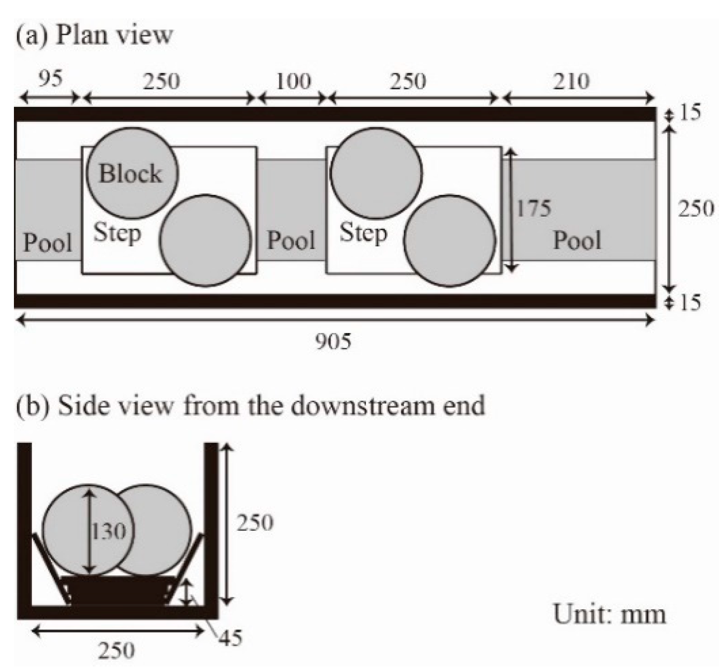
Figure 2.
Computational domain of drainage canal without fishway. (a) Plan view of the whole domain. (b) Longitudinal cross section A-Aʹ. (c) Transverse cross section B-B ʹ. (d) Transverse cross section C-Cʹ.
Figure 2.
Computational domain of drainage canal without fishway. (a) Plan view of the whole domain. (b) Longitudinal cross section A-Aʹ. (c) Transverse cross section B-B ʹ. (d) Transverse cross section C-Cʹ.
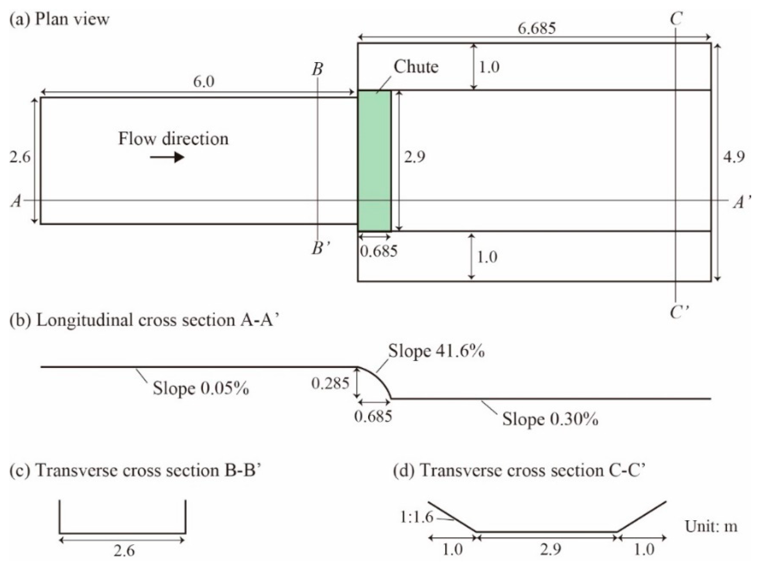
Figure 3.
Portable fishway with a catching wire net located on the chute on the right side of the bank. Flow is from back to front. The hanging plants along the left-bank side wall in the upstream canal section reach the water surface.
Figure 3.
Portable fishway with a catching wire net located on the chute on the right side of the bank. Flow is from back to front. The hanging plants along the left-bank side wall in the upstream canal section reach the water surface.
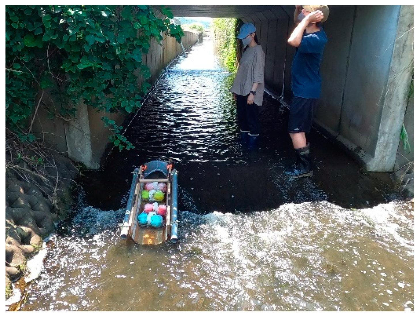
Figure 4.
Zoom-in photo of the portable fishway positioned on the left side of the bank of the drainage canal.
Figure 4.
Zoom-in photo of the portable fishway positioned on the left side of the bank of the drainage canal.
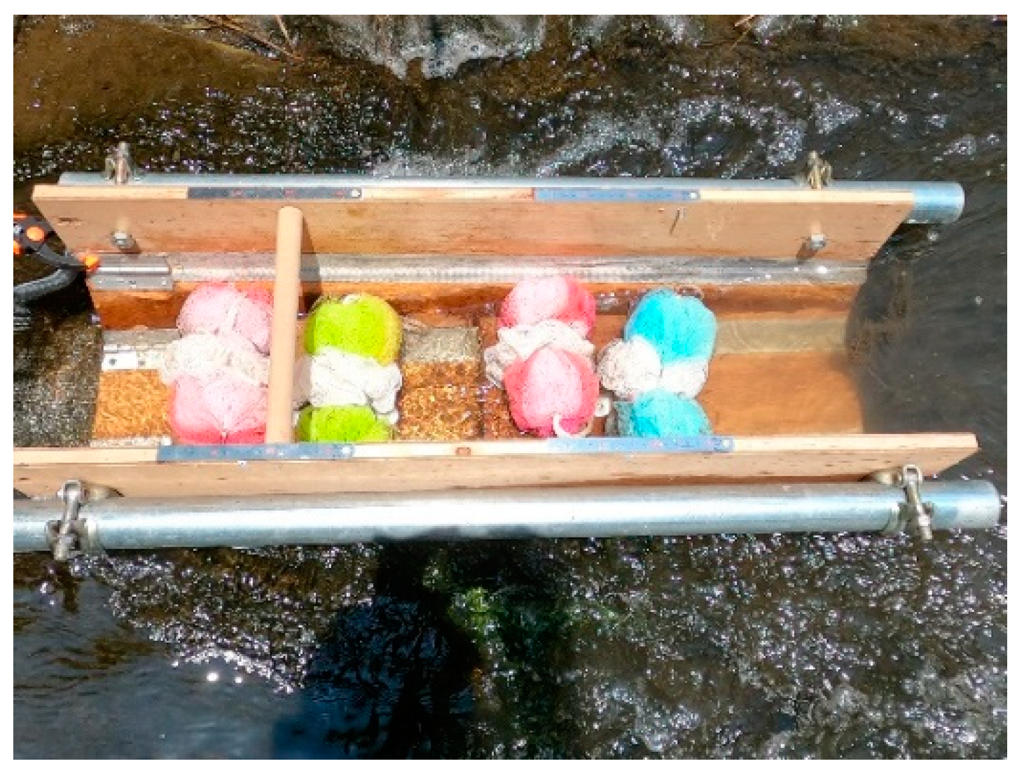
Figure 5.
Monitoring points in the portable fishway (1–19) and the canal (20–31).
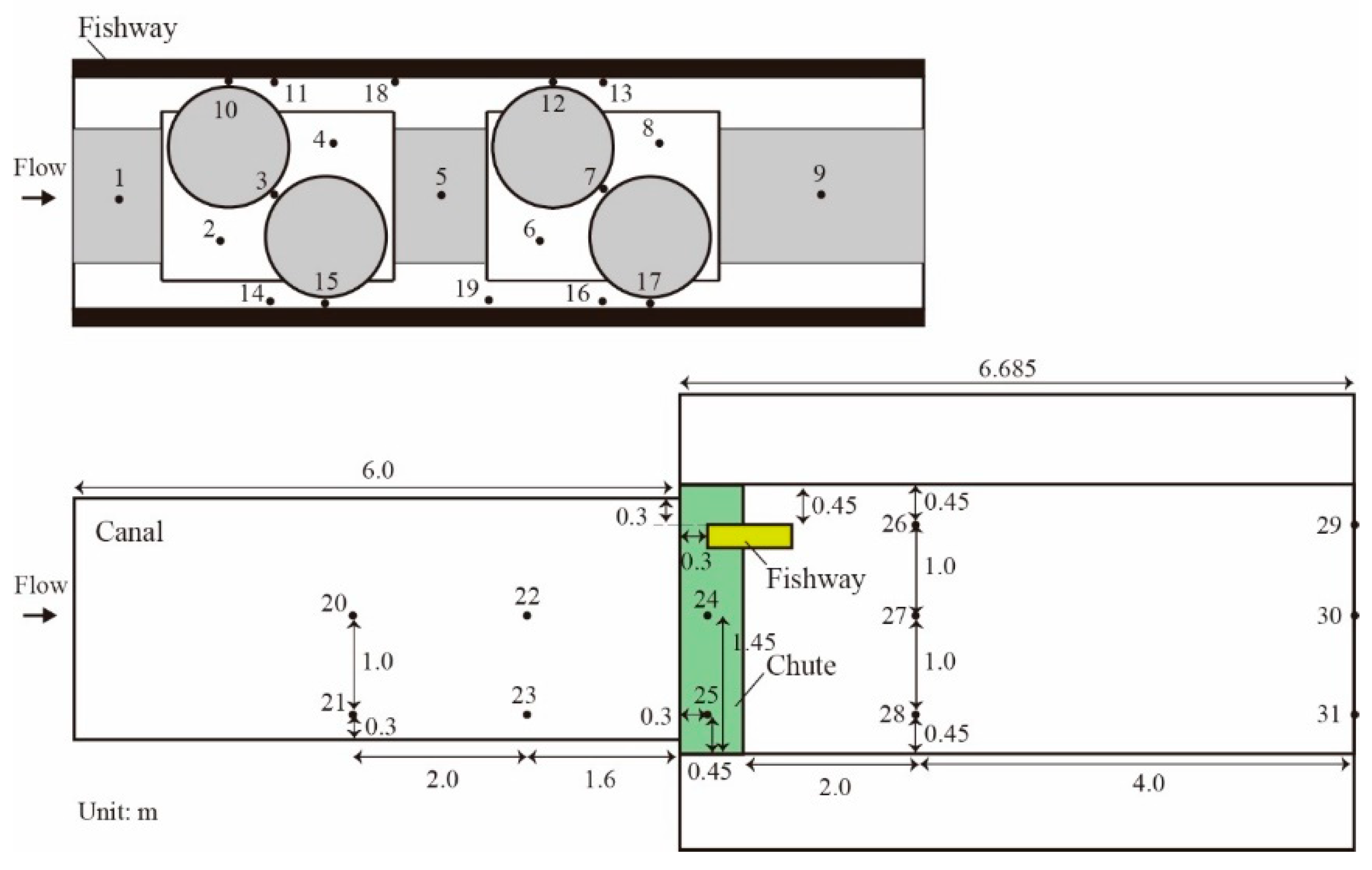
Figure 6.
Computational domain of drainage canal with fishway located on chute. Every case of location of fishway is illustrated.
Figure 6.
Computational domain of drainage canal with fishway located on chute. Every case of location of fishway is illustrated.
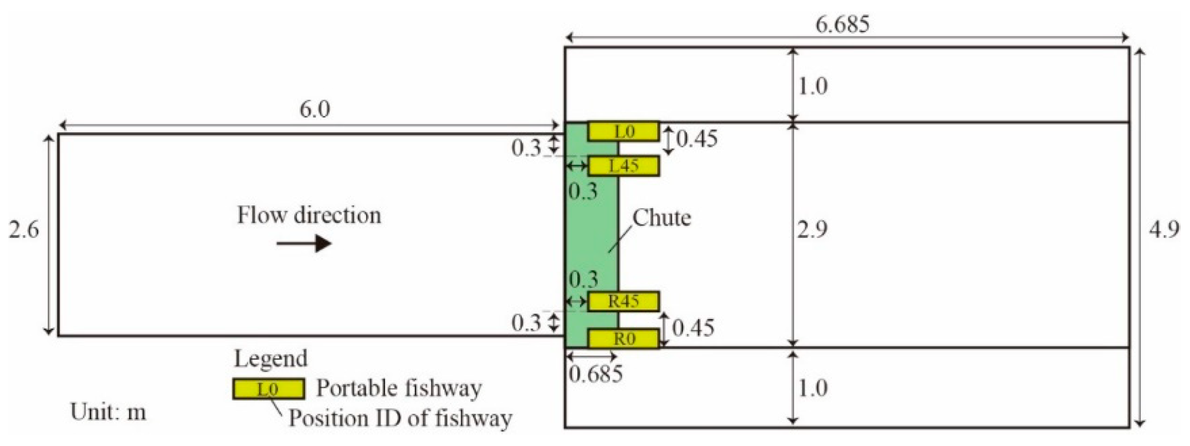
Figure 7.
Computational mesh around the portable fishway in Case L0_0.265. Flow direction is from left to right. Two red parallel lines indicate sidewalls of the fishway.
Figure 7.
Computational mesh around the portable fishway in Case L0_0.265. Flow direction is from left to right. Two red parallel lines indicate sidewalls of the fishway.
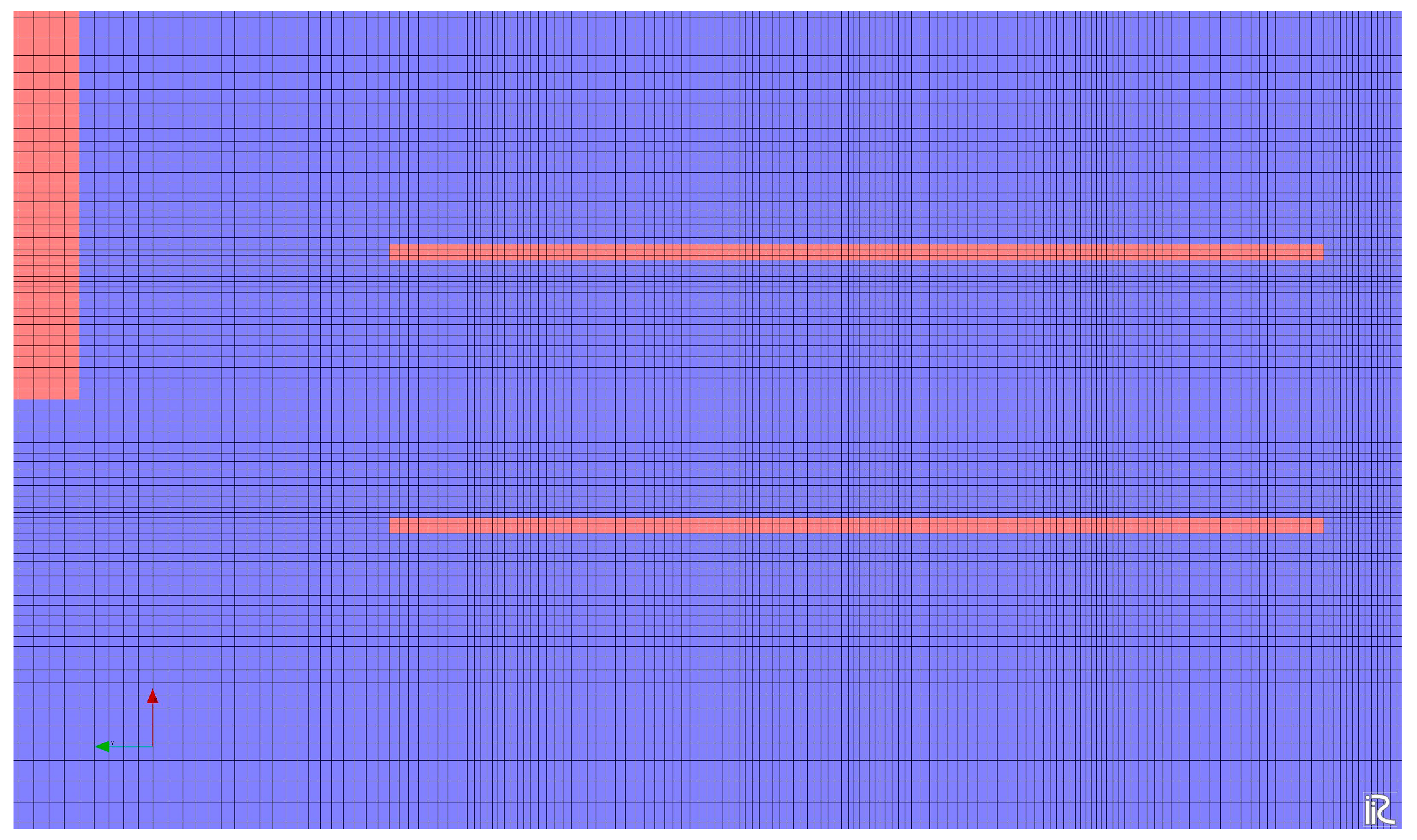
Figure 8.
Juvenile Rhinogobius sp. OR caught in the portable fishway system on June 10, 2021.
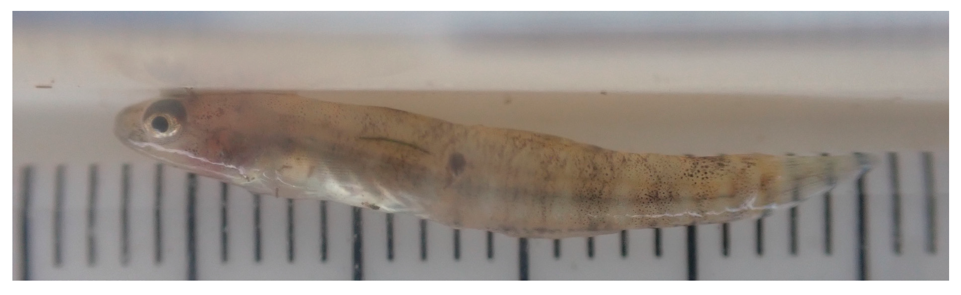
Figure 9.
Observed water depth and current velocity under a discharge of 0.140 m3s−1 in the portable fishway (monitoring points 1–19) and canal (monitoring points 20–31).
Figure 9.
Observed water depth and current velocity under a discharge of 0.140 m3s−1 in the portable fishway (monitoring points 1–19) and canal (monitoring points 20–31).
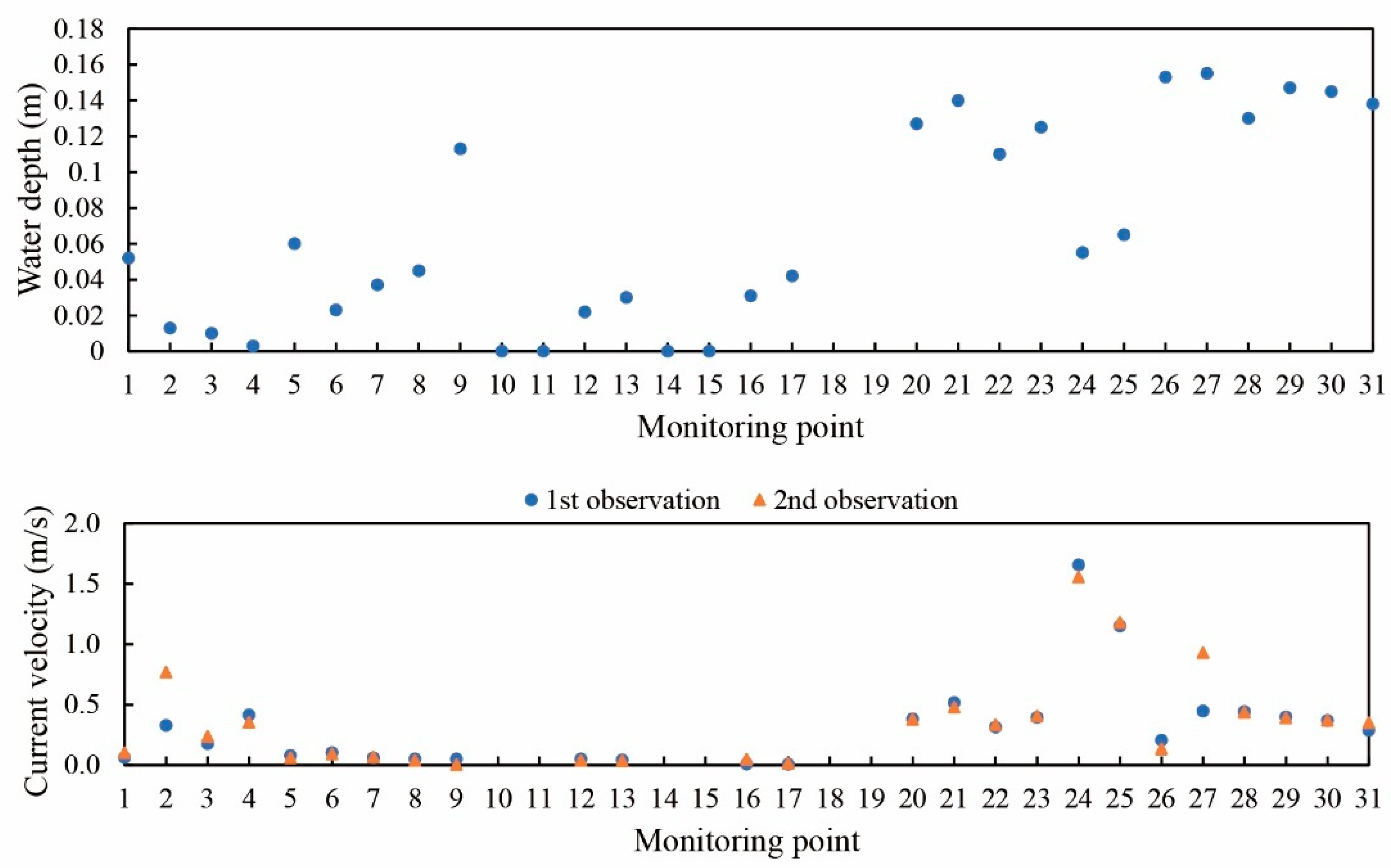
Figure 10.
Computed water depth and current velocity under a discharge of 0.140 m3s−1 at the monitoring points in the portable fishway in Cases L0_0.140, L45_0.140, R0_0.140 and R45_0.140.
Figure 10.
Computed water depth and current velocity under a discharge of 0.140 m3s−1 at the monitoring points in the portable fishway in Cases L0_0.140, L45_0.140, R0_0.140 and R45_0.140.
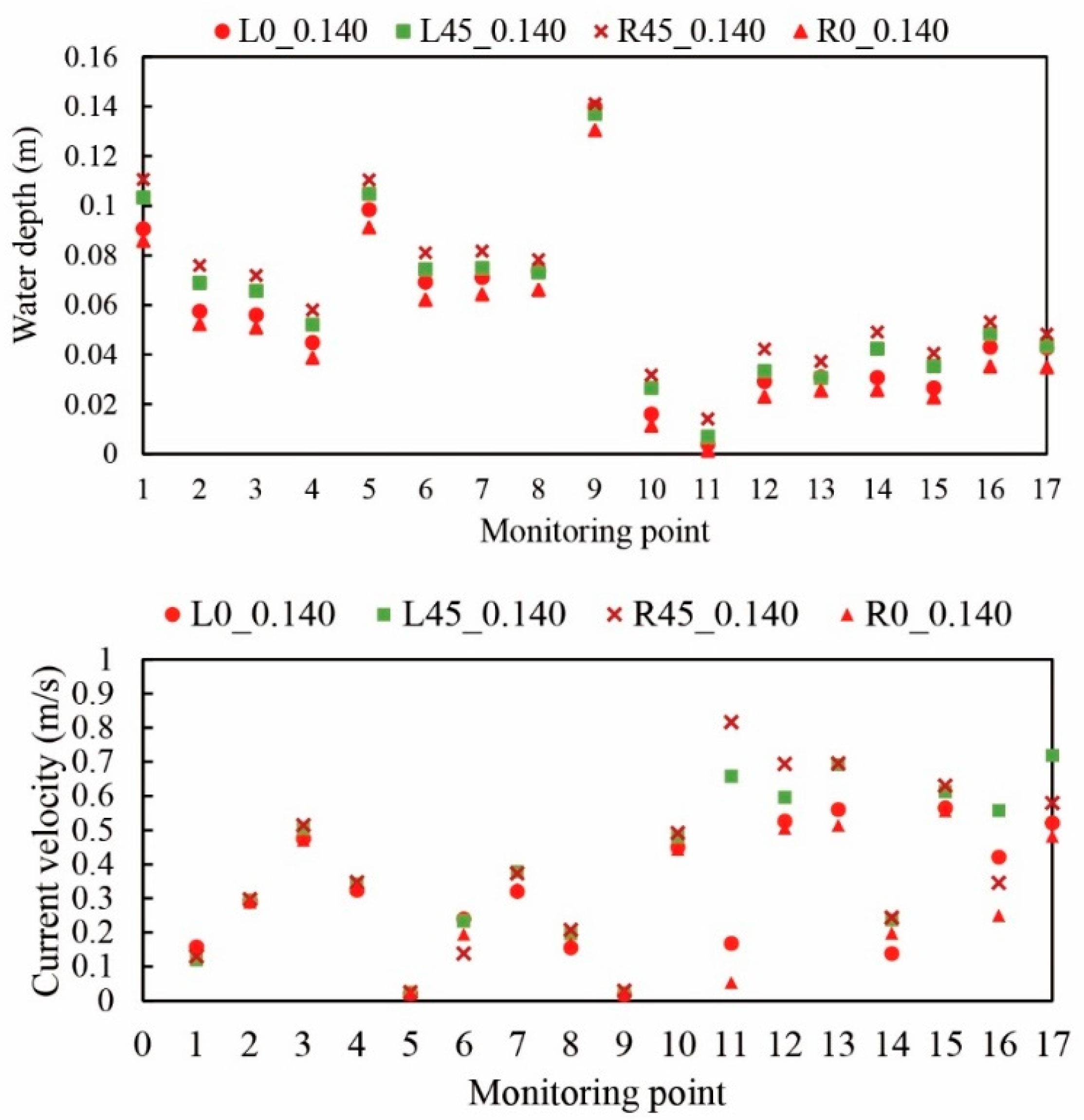
Figure 11.
Computed water depth (> 5 mm) across the entire computational domain under a discharge of 0.140 m3s-1. In each panel, the central part represents the chute in the canal. In panels (b) through (e), the sidewalls of the portable fishway are depicted by two horizontal, parallel white lines on the chute.
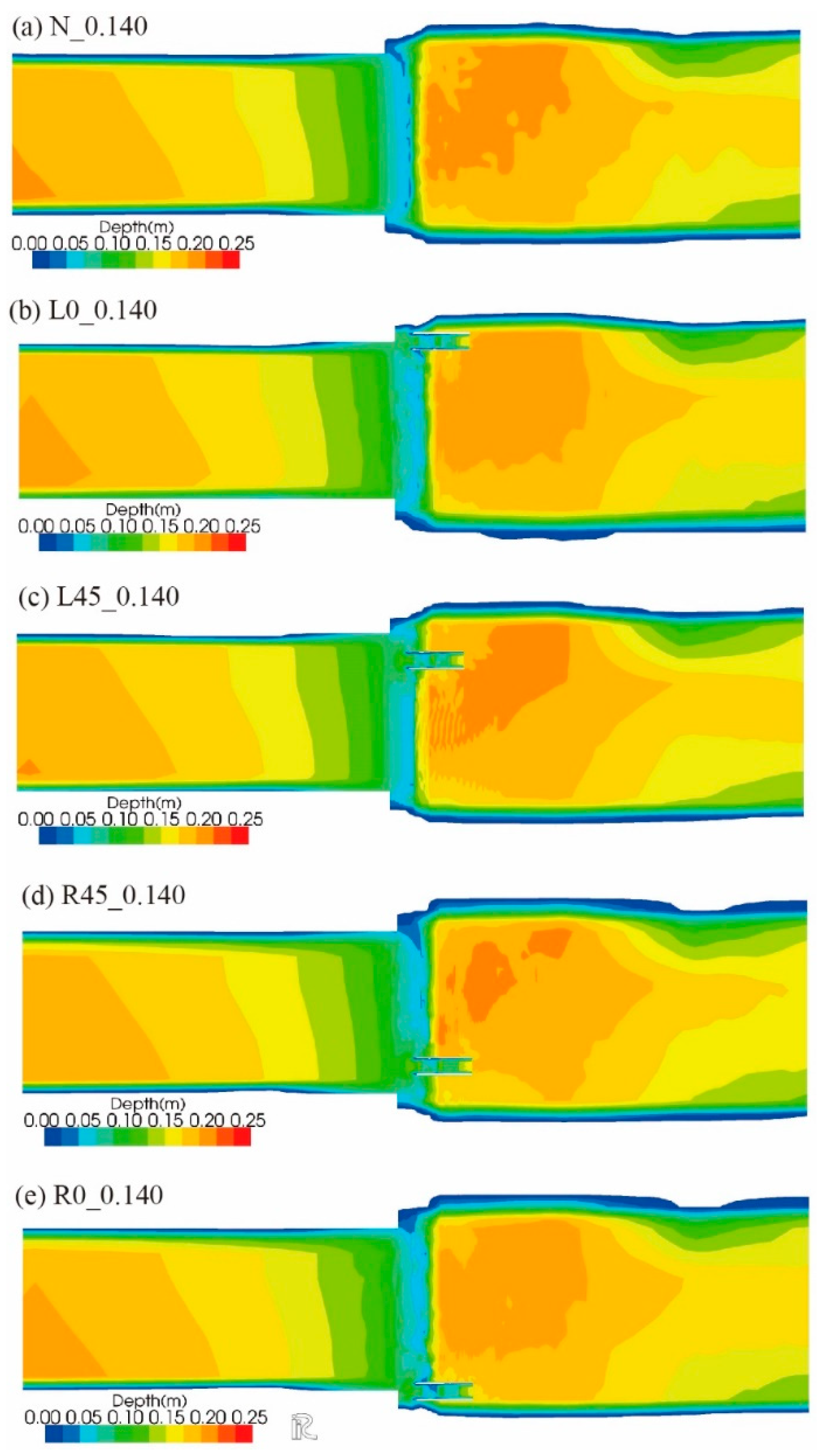
Figure 12.
Computed current velocity in the canal in and around the chute under a discharge of 0.140 m3s−1.
Figure 12.
Computed current velocity in the canal in and around the chute under a discharge of 0.140 m3s−1.
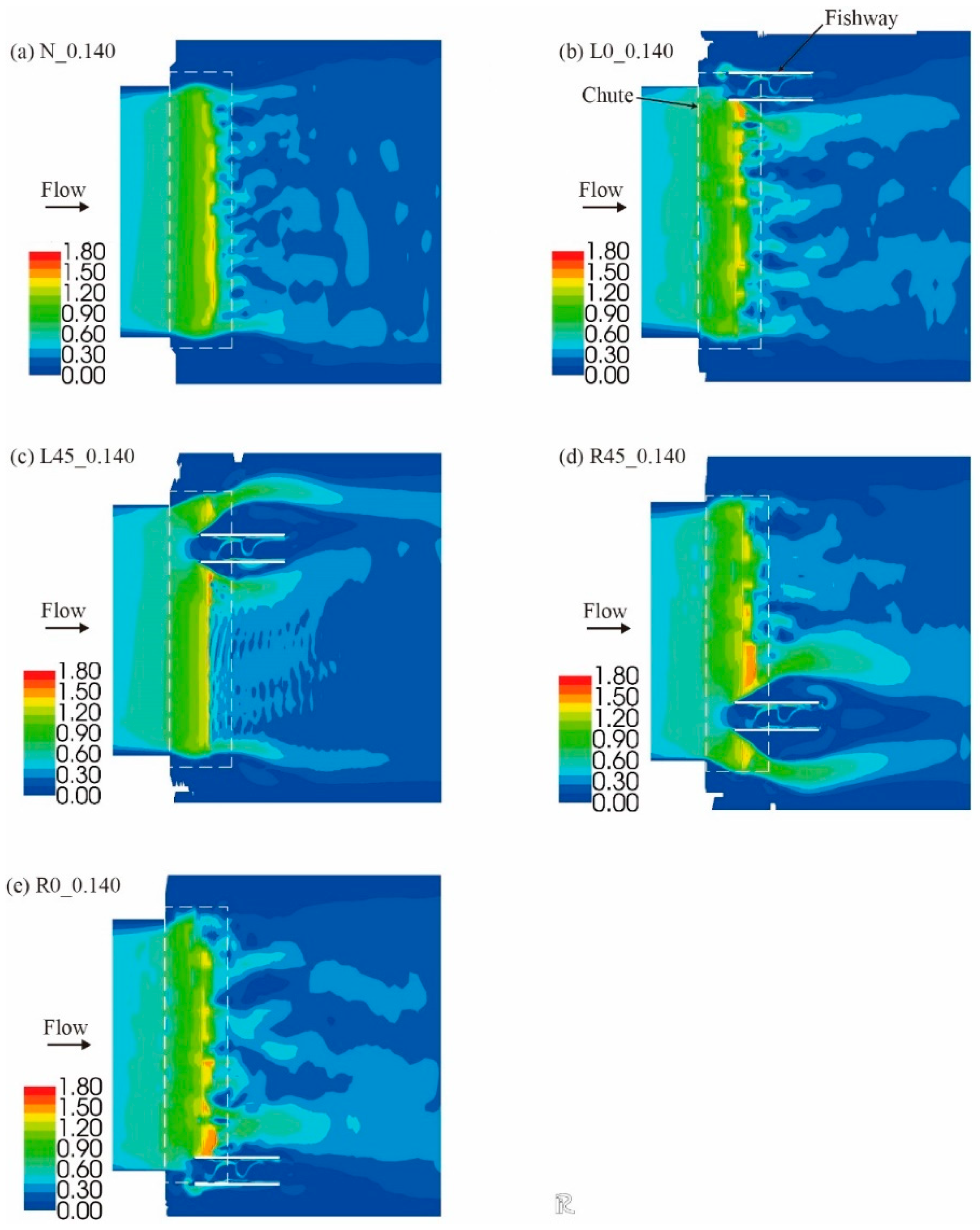
Figure 13.
Computed water depth (> 5 mm) across the entire computational domain under a discharge of 0.265 m3s−1. In each panel, the central part represents the chute in the canal. In panels (b) through (e), the sidewalls of the portable fishway are depicted by two horizontal, parallel white lines on the chute.
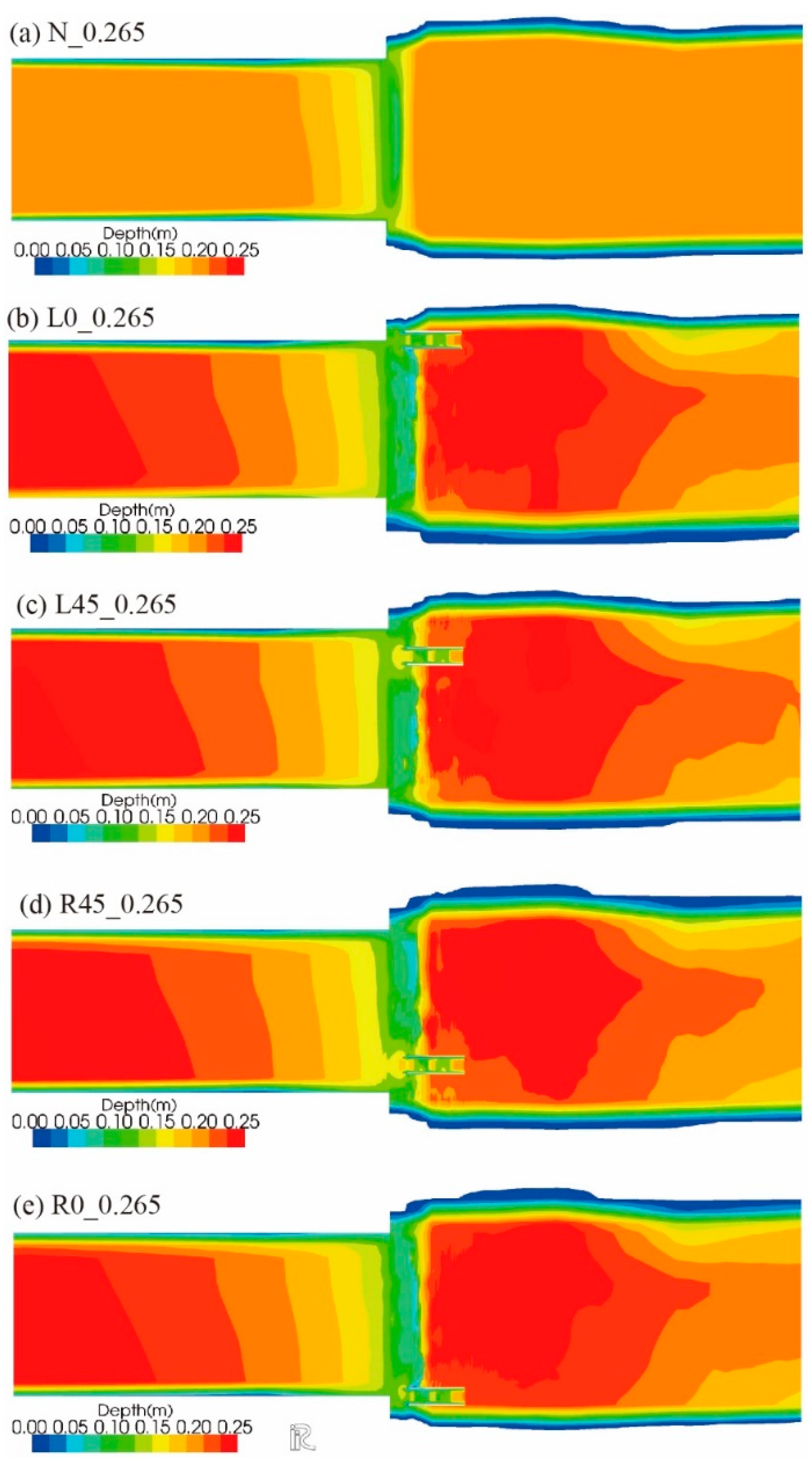
Figure 14.
Computed current velocity in the canal in and around the chute under a discharge of 0.265 m3s−1.
Figure 14.
Computed current velocity in the canal in and around the chute under a discharge of 0.265 m3s−1.
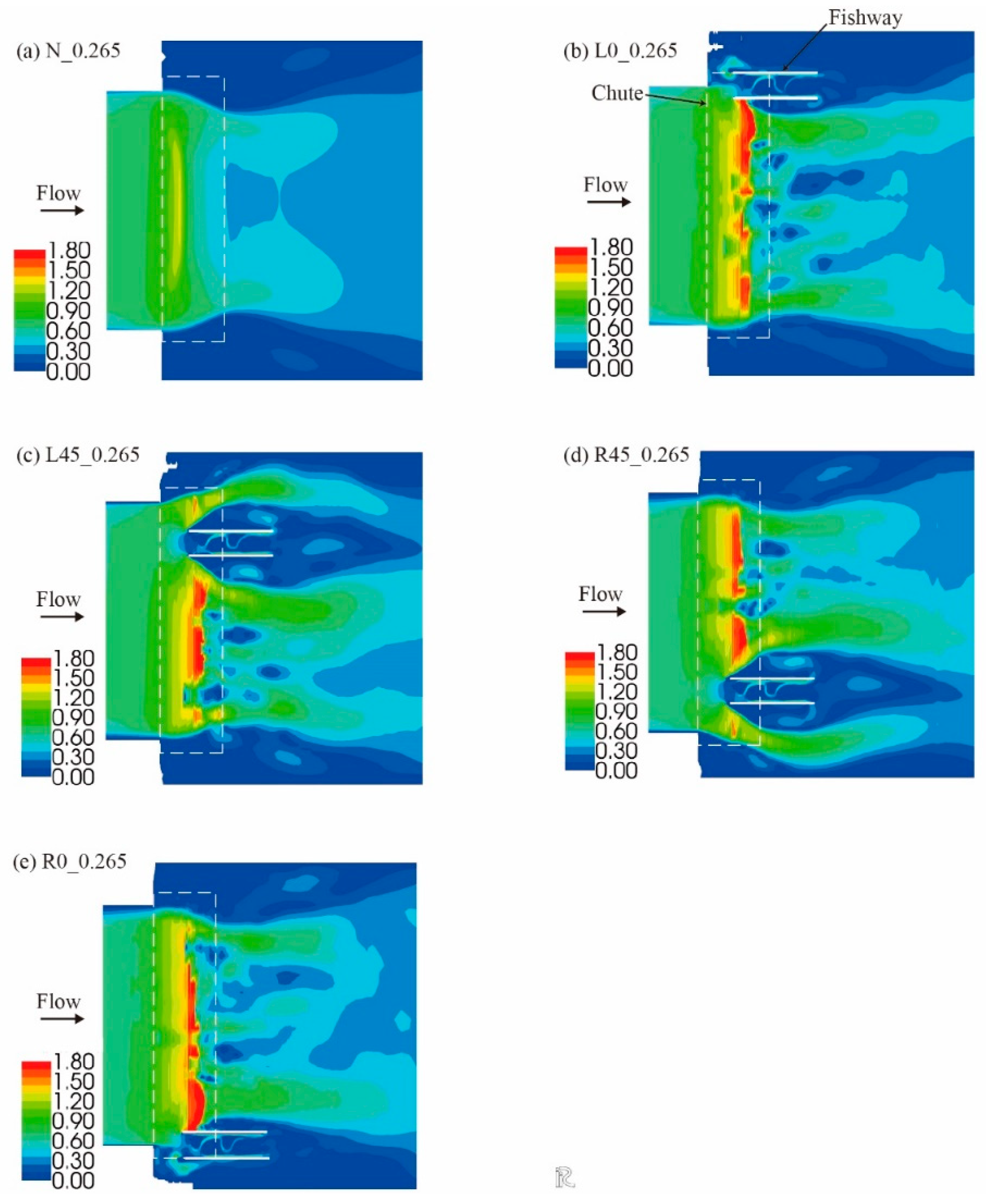
Figure 15.
Computed streamlines around the portable fishway in the canal at a discharge of 0.140 m3s−1.
Figure 15.
Computed streamlines around the portable fishway in the canal at a discharge of 0.140 m3s−1.
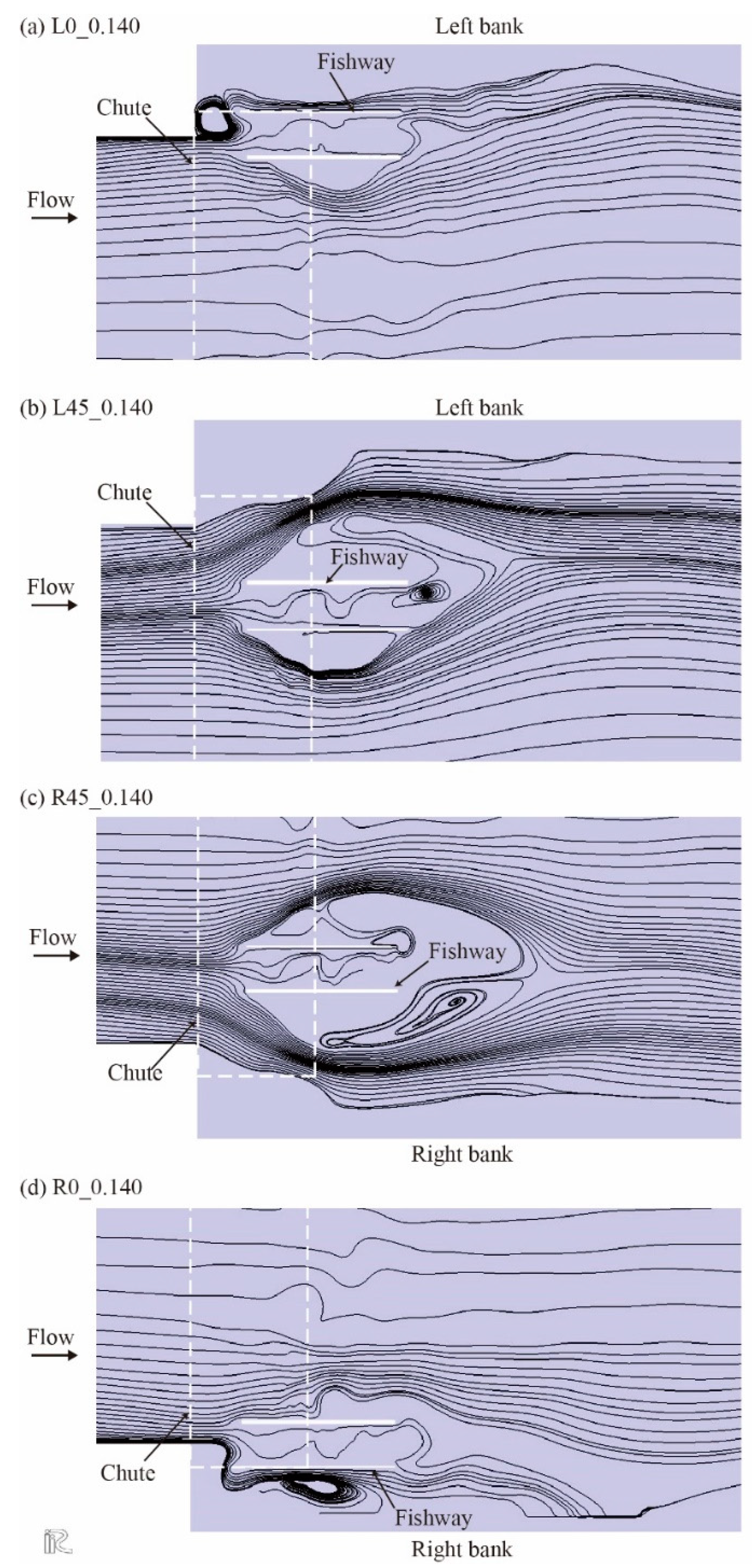
Figure 16.
Computed streamlines around the portable fishway in the canal at a discharge of 0.265 m3s−1.
Figure 16.
Computed streamlines around the portable fishway in the canal at a discharge of 0.265 m3s−1.
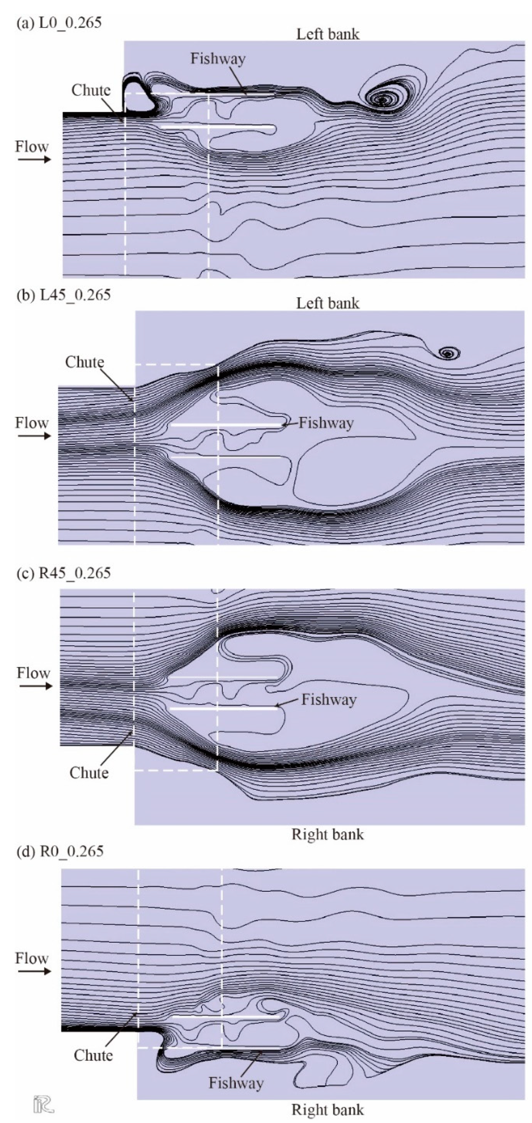
Figure 17.
Computed velocity vectors and velocity magnitude focused in and around the fishway in Case L0_0.265.
Figure 17.
Computed velocity vectors and velocity magnitude focused in and around the fishway in Case L0_0.265.
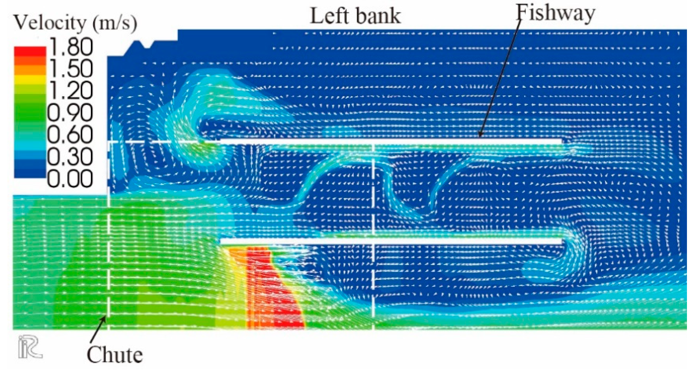

Table 1.
Specifications of portable electromagnetic current meter used in this study.
| Item | Explanation |
|---|---|
| Measuring direction | 3 axes 6 directions |
| Flow range | −2 to +2 m/s |
| Accuracy | ± 0.010 m/s (velocity range: 0 to ± 0.499 m/s), ± 0.020 m/s (velocity range: ± 0.500 to ± 0.999 m/s), ± 0.040 m/s (velocity range: ± 1.000 to ± 2.000 m/s) |
| Noise | Within ±0.005 m/s under hydrostatic condition |
| Response time | 0.5 s |
Table 2.
Computational conditions for model calibration, validation, and configuration of the portable fishway.
Table 2.
Computational conditions for model calibration, validation, and configuration of the portable fishway.
| Case | Upstream discharge (m3s−1) | Downstream water depth (m) | Position of fishway | Number of nodes | Note |
|---|---|---|---|---|---|
| N_0.140 | 0.140 | 0.143 | No fishway | 11,685 (= 123 × 95) |
|
| N_0.210 | 0.210 | 0.149 | No fishway | 11,685 (= 123 × 95) |
Validation |
| N_0.265 | 0.265 | 0.187 | No fishway | 11,685 (= 123 × 95) |
|
| L0_0.140 | 0.140 | 0.143 | On left bank | 50,024 (= 338 × 148) |
|
| L0_0.265 | 0.265 | Uniform depth | On left bank | 50,024 (= 338 × 148) |
|
| L45_0.140 | 0.140 | 0.143 | 0.45 m away from left bank | 59,312 (= 337 × 176) |
Calibration |
| L45_0.265 | 0.265 | Uniform depth | 0.45 m away from left bank | 59,488 (=338 × 176) |
|
| R0_0.140 | 0.140 | 0.143 | On right bank | 50,024 (= 338 × 148) |
|
| R0_0.265 | 0.265 | Uniform depth | On right bank | 50,024 (= 338 × 148) |
|
| R45_0.140 | 0.140 | 0.143 | 0.45 m away from right bank | 71,136 (= 342 × 208) |
|
| R45_0.265 | 0.265 | Uniform depth | 0.45 m away from right bank | 71,136 (= 342 × 208) |
Disclaimer/Publisher’s Note: The statements, opinions and data contained in all publications are solely those of the individual author(s) and contributor(s) and not of MDPI and/or the editor(s). MDPI and/or the editor(s) disclaim responsibility for any injury to people or property resulting from any ideas, methods, instructions or products referred to in the content. |
© 2023 by the authors. Licensee MDPI, Basel, Switzerland. This article is an open access article distributed under the terms and conditions of the Creative Commons Attribution (CC BY) license (http://creativecommons.org/licenses/by/4.0/).
Copyright: This open access article is published under a Creative Commons CC BY 4.0 license, which permit the free download, distribution, and reuse, provided that the author and preprint are cited in any reuse.


