
Submitted:
21 October 2023
Posted:
23 October 2023
You are already at the latest version
Abstract
This study presents a research plan that utilizes data obtained from wearable devices to
identify human activities and gain insights into human behavior. We developed a model capable of
classifying activities similar to human behavior and evaluated the effectiveness and generalization
capabilities of this model. The data underwent initial preprocessing, including standardization and
normalization. Additionally, recognizing the inherent similarities between human activity behaviors,
we introduced a multi-layer classifier model. The first layer is a random forest model based on
stepwise regression, which may encounter reduced accuracy for similar activities. The second layer
employs a Support Vector Machine (SVM) model based on Kernel Fisher Discriminant Analysis
(KFDA). KFDA is used to reduce the dimensionality of data points with potential confusion,
followed by SVM for classification. The model was experimentally evaluated and applied to four
benchmark datasets: UCI DSA, UCI HAR, WISDM, and IM-WSHA. The experimental results
demonstrate that our approach achieved recognition accuracies of 99.71%, 98.71%, 99.12%, and
97.6% on these datasets, indicating excellent recognition performance. Furthermore, to assess the
model's generalization ability, we performed K-fold cross-validation on the random forest model
and utilized ROC curves for the SVM classifier. The results indicate that our multi-layer classifier
model exhibits robust generalization capabilities.
Keywords:
body-worn sensors
; multi layer classifier
; random forest
; kernel fisher discriminant analysis
; SVM
; stepwise regression
1. Introduction and Related Work
Human Activity Recognition (HAR) involves identifying various human behaviors through a series of observations of individuals and their surrounding environment [39]. HAR has been generally applied in many fields, such as Security and Surveillance[40], sports and fitness[41], industry and manufacturing[42], autonomous driving[44],and the references therein.
A novel IoT-perceptive human activity recognition (HAR) approach using multihead convolutional attention in [1].Hand-crafted and deep convolutional neural network features fusion and selection strategy in [2].In [3], authors consider smart homes environments using Lstm networks.In [4], using A federated learning system with enhanced feature extraction to Human Activity Recognition and using Bi-LSTM network for multimodal continuous human activity recognition and fall detection [5].In the field of industry and manufacturing, Utilizing time factor analysis in conjunction with human action recognition for worker operating time [6] and applying deep learning to human activity recognition [7] etc., they rely heavily on HAR technology which improves the accuracy of targeting criminals [8].In the field of autonomous driving [9], the recognition of human activities will help to develop a suitable autonomous driving system.
Human activity recognition (HAR) methods can be broadly categorized into two main directions: 1) vision-based HAR and 2) wearable sensor-based HAR. It is well-known that vision-based HAR is generally considered more advanced compared to wearable sensor-based HAR [10]. but, vision-based HAR also faces several challenges. For one thing, there are privacy concerns related to the potential leakage of video data, and image processing demands significant computational power and substantial storage resources. For another, factors such as the observer's position and angle, the subject's physique, attire, background color, and light intensity can all impact the accuracy of vision-based HAR [11].In contrast, inertial sensor technology is typically cost-effective and offers greater robustness and portability in various environmental conditions [12]. Currently, sensor-based recognition technology has gained widespread attention due to its superior confidentiality and relatively lower computational requirements. Therefore, in [13], the authors discussed the role of sensor placement in the design of HAR systems to optimize their availability. Leveraging these advantages, wearable sensor-based HAR has garnered increasing interest in recent years.
In recent years, wearable sensor-based HAR has gained widespread attention. The earliest research on sensor-based recognition of human behavior can be traced back to the 1990s, with studies by researchers such as F. Foerster [21] and O. X. Schlmilch [22]. Nowadays, wearable sensor research has yielded many high-accuracy models. For example, Bao and his team achieved an overall accuracy of 84% through effective data collection and decision tree classification [23]. The Centinela system developed by D. Lara and colleagues achieved an overall accuracy of 95.7% [24]. However, at the same time, a problem has been identified where single classification models can lead to significant confusion when distinguishing similar activities (such as ascending stairs and descending stairs).In the study by JANSIR et al. [14], they employed chaotic mapping to compress raw tri-axial accelerometer data and extracted 38 time-domain and frequency-domain features, including mean, standard deviation, root mean square, dominant frequency coefficient, spectral energy, and others. They achieved a recognition accuracy of 83.22% in human activity recognition. However, the results showed significant confusion between activities such as running, ascending stairs and descending stairs. In the research by VANRELLS et al. [15], they extracted a 91-dimensional feature vector from single-axis accelerometer data, including cepstral coefficients, time-domain features, and periodicity features. They achieved a recognition accuracy of 91.21% in a classification task involving ten different human activities. However, the results also indicated substantial confusion between activities such as cycling on an exercise bike in horizontal, cycling on an exercise bike in vertical positions, ascending stairs and descending stairs. The reasons for the confusion between similar activities can be summarized in two aspects. Firstly, within the same individual, different activities may share similar activity cycles or amplitudes, leading to activity recognition confusion and a decrease in overall accuracy.
Kernel Fisher Discriminant Analysis (KFDA) is a powerful extension of Fisher Discriminant Analysis (FDA) [45] that has proven to be highly effective in various pattern recognition and classification tasks. While traditional FDA is primarily designed for linearly separable data, KFDA extends its capabilities by allowing the analysis of nonlinearly separable data through the use of kernel functions.It serves as a robust nonlinear classifier suitable for tackling pattern recognition, classification, and regression analysis tasks[46].The KFDA method is capable of reflecting the nonlinear relationships between the input and output variables of the dataset, and shows good generalisation performance in many practical problems.
We have noticed the success of Shaoqun Dong and colleagues [43] in addressing similar Lithofacies identification problems, and we also intend to employ kernel Fisher discriminant analysis to preprocess similar issues before proceeding with data classification. Nowadays, there are numerous applications of kernel Fisher discriminant analysis in the field of machine learning as well. For instance, Liu et al. [47] have used this technique to enhance tasks like face recognition.
To address the issue of confusion between similar activities in single-model human activity recognition and enhance the overall recognition accuracy of multi-class activities, we drew inspiration from the success of Shaoqun Dong [43] and others in solving similar Lithofacies identification problems. We decided to leverage KFDA to preprocess the similar activity data before performing classification. In this paper, we propose a multi-layer neural network model based on Kernel Fisher Discriminant Analysis. This approach comprises preprocessing steps, followed by initial classification using Random Forest. Subsequently, KFDA is applied to process the data. Finally, SVM are employed for detailed classification of ambiguous actions. The end result is a robust neural network classification model that effectively addresses the challenge of distinguishing similar activities.
Therefore, the main contributions of this paper can be summed up as follows:
- 1)
- We propose a model design aimed at addressing the issue of confusion between similar activities.
- 2)
- To tackle the problem of similar activity feature similarity, we introduce an SVM neural network classification approach based on Kernel Fisher Discriminant Analysis, which effectively classifies similar activities.
- 3)
- Additionally, we conducted classification experiments on four common benchmark datasets and performed detailed analyses on these datasets. We compared our model with mainstream classification models. Experimental results demonstrate that our model exhibits excellent classification performance.
The remaining sections of this paper are organized as follows. Section II provides a brief introduction to the work carried out in this paper, along with details about the dataset used. Section III conducts a basic data analysis and employs appropriate data preprocessing techniques. Section IV introduces our proposed human motion approach based on a multi-layer classifier. Section V presents the experimental setup, provides results for our proposed method on multiple datasets, and offers an analysis and discussion of these results. Finally, in Section VI, we summarize the insights gathered from these experiments and outline future directions.
2. Word
In the field of HAR research, various datasets have been previously published. Notable among them is the UCI (University of California, Irvine) HAR dataset, recognized for its widespread utilization in numerous studies and comparisons [48]. Additionally, the WISDM (Wireless Sensor Data Mining) dataset [17] is also prominently featured. Furthermore, datasets such as UCI DSA [16] and IM-WSHA [18], which are both accessible through UCI, have been employed. In addition to these, there exist several other datasets that are not individually detailed within this article. Subsequent sections will provide a comparative analysis of the strengths and weaknesses of these three primary datasets, as presented in Table 1.
To highlight these differences, a qualitative comparison between these three datasets is presented in Table 1.
While the data collected from UCI DSA may appear simpler in comparison to WISDM and UCI ADL, UCI HAR captures a wide range of 19 different human activities. Unlike other datasets, it better represents complex human activities and serves as a more comprehensive showcase for our model in this paper. We conducted experiments using the four aforementioned databases, but in the following sections, we focus our narrative on UCI DSA.
The UCI DSA data in this paper were obtained from measurements of human activity by miniature inertial sensors and magnetometers in different parts of the body. Sensor data were collected from a total of 8 subjects performing 19 different activities. The total signal duration for each subject for each activity was 5 minutes. The sensor unit was calibrated to acquire data at a 25 Hz sampling frequency. The 5-minute signal was divided into 5-second segments, resulting in 480 (=60 × 8) signal segments for each activity.
A total of eight volunteers participated, resulting in a collection of 9120 instances. This dataset elaborately describes the data captured from various sensors, measuring activities performed by different subjects within the same time intervals. We consolidated this textual dataset into a CSV file comprising two columns: subject ID and activity type.
After data pre-processing, based on the filtered features, our team designed a feasible algorithmic solution to classify 19 human behaviors. Due to the particularly large amount of data and the inherent similarity of human activities, direct classification of the 19 human behaviors using a single machine learning algorithm would easily result in confusion of similar behaviors and lead to degradation of classification accuracy.
To provide a clearer presentation of our solution, our team utilizes Figure 2.1 and employs a flowchart to illustrate the framework of our approach.
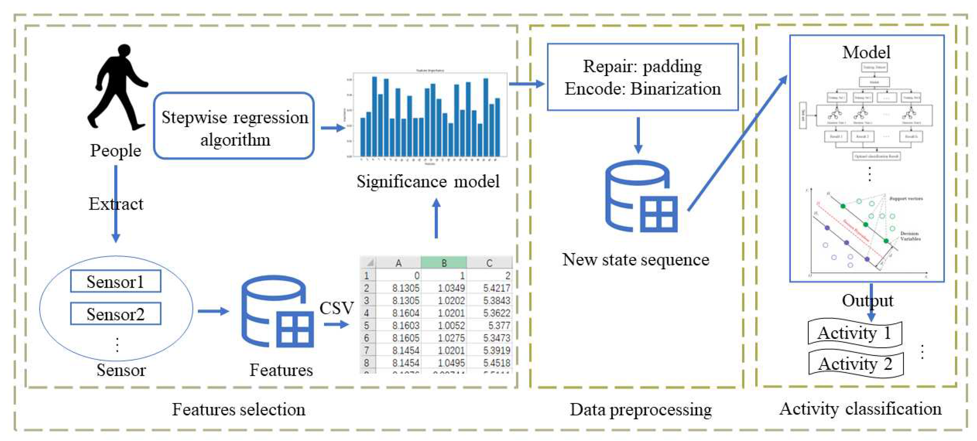
Figure 1.
Overview of the system workflow.
After data preprocessing and based on the selected features, our team devised a viable algorithmic solution. Initially, all activity data underwent a first-level classification using Random Forest. Subsequently, kernel Fisher discriminant analysis was applied to reduce dimensionality for activities prone to confusion, followed by further fine-grained classification using Support Vector Machines (SVM). This iterative process continued until no more instances of confounding activities were encountered.
In order to provide a more detailed overview of our efforts in addressing similar activities and how we distinguish other actions within confusing scenarios, we have created the following diagram to illustrate our Model:
3. Method and data preprocessing
3.1. Intuitive Data Processing
In this section, the preprocessing work, to avoid unnecessary complexity in the article, is illustrated using the UCI DSA dataset as an example. We downloaded the dataset from the official UCI website [16] and found it to be somewhat disorganized. To streamline the dataset, we consolidated the original files into a CSV file. Additionally, to simplify the lengthy labels under the "Behavior" column in the dataset, as discrete information such as IDs and names are not needed for the actual experiments, we adopted an abbreviated format. This processing aligns with the original dataset, for instance, replacing "sitting" with "A1." For detailed information, please refer to Table 2.
3.2. Standardisation and normalisation
we examined the data samples by randomly selecting a metric and presenting it alongside 19 different activities. As shown below, we preprocessed the data through standardization and normalization methods. In Figure 3(a), the original data for this metric, comprising 60,000 sample points across various activities, is displayed. After our preprocessing, as depicted in Figure 3(b), it is evident that all data now falls within the range of 0 to 1, while preserving the fundamental characteristics of the data.
4.1. Random Forest initial classification model base on stepwise regression
Firstly, the SR-Random Forest model is proposed by combining the stepwise regression analysis with the Random Forest model. Then, the KFDA-SVM Model is proposed by combining the kernel Fisher discriminant analysis with SVM. In this section, firstly, the stepwise regression algorithm and the Random Forest Model are introduced and the SR-Random Forest Model is proposed, and furthermore, the kernel Fisher discriminant analysis model and SVM model and gives their combined model.
In order to obtain a higher initial classification accuracy for subsequent improvement in the second classification stage . In [58], it is mentioned that the use of feature selection algorithms will be able to effectively improve the efficiency of machine learning, so we first extract the relevant metrics using stepwise regression to calculate the importance of the input metrics. Random forest is an ensemble classifier that uses multiple decision trees to train samples and make predictions. In this section, the SR -RF model is shown in Figure 4.
4.1.1. Stepwise regression algorithm
Stepwise regression analysis algorithms can be traced back to the 19th century statistician and mathematician Francis Galton, however, the formal development and promotion of stepwise regression can be traced back to the 20th century statisticians and mathematicians, especially R. A. Fisher, In this paper, we use stepwise regression analysis to analyse the 45 indicators in the UCI DSA (g1,g2,...g45) rows of stepwise regressions. analyses, and we also chose a variable y as the response variable. It is assumed that the indicators satisfy equation (1):
y = α0 + α1g1 + α2g2 + ... + ε
Assuming that there is a linear relationship between and , , and substituting it
into equation (1), we get
y = α0 + bα2 + (α1+αα2)g1 + ... + α2v
Suppose that Eq:
The estimation of model (3) is
The sum of squared residuals for model (3) is
The sum of squared residuals for model (1) is
Comparing Q1 and Q3, Q1−Q3≈0, it is possible to eliminate g1. The stepwise regression method can effectively reduce the number of features in the data, improving the fitting performance of the model.
4.1.1. Stepwise regression algorithm
The main features that can classify human behavior have been extracted in the above steps. Considering the relationship between these data and the fact that the samples used for training are discrete and the amount of data is huge, the random forest algorithm is considered for network training, and its general algorithmic flow is shown in Figure 5. In order to initially identify multi-class activities, the random forest classification algorithm with excellent performance in supervised learning is chosen for the layer 1 classifier.
4.1.2. Random forest base on Stepwise regression algorithm
Random Forest is a composite classification model composed of many decision tree classification models {H(X,Θk),k=1,...}, and the parameter set {Θk} is a collection of independently and identically distributed random vectors. Under the given independent variables X, each decision tree classification model selects the optimal classification result through a majority vote. The basic idea is to first use bootstrap sampling to extract k samples from the original training set, with each sample having the same sample size as the original training set. Then, k decision tree models are built for the k samples, resulting in k different classification results. Finally, based on these k classification results, a majority vote is used to determine the final classification result for each record.
The final classification decision in a random forest is made by training through k rounds, obtaining a sequence of classification models {h1(X),h2(X),...hk(X)}, and using them to create a multi-classification model system. The ultimate classification result of this system is determined using a simple majority voting method:
where, H(x) is a multi-classification model, hi is an individual decision tree classification model, and Y represents the output variable.
The specific implementation of the above ideas, as illustrated in Algorithm 1, combines stepwise regression and random forest modeling to create a novel classification model. Its advantage lies in the ability to select features from the classification dataset effectively.
| Algorithm 1: Random Forest Model base on Stepwise regression algorithm |
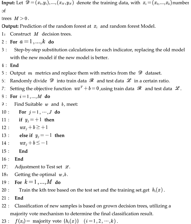 |
4.2. Second layer SVM classification Base kernel Fisher discriminant analysis
To address the issue of similarity between two easily confused types of actions, we employed two key steps. First, we utilized KFDA for feature dimensionality reduction, effectively separating similar activities. This step aims to increase the distance between different actions in the data space, thereby facilitating subsequent SVM classification. Let's delve into the principles and workflow of these two steps in more detail. Firstly, we will introduce KFDA, and then we will provide a deeper explanation of SVM. This process's workflow is analogous to the one depicted in Figure 6.
4.2.1. Principle of kernel Fisher discriminant analysis
KFDA is a pattern recognition and classification method based on kernel techniques and is an extension of Fisher Discriminant Analysis. KFDA is designed to handle nonlinearly separable data by mapping the data to a high-dimensional feature space, thereby improving classification performance. We describe KFDA in conjunction with [43] Kernel Fisher Discriminant Analysis (KFDA) was first proposed by Schölkopf et al. in 1997 [52] and can be expressed as the maximisation equation (7):
wherein, SW represents the within-class
scatter matrix, Sb is the between-class scatter matrix, and denotes the
projection vector.
The above problem can be equated to finding the generalised eigenvectors of the eigenvalue problem:
where the eigenvalues λi represent the discriminative power of each projection vector. Once we obtain the projected vector v, it can be used for classification instead of the original vectors with a linear classifier.
The limitations of the LDA method are primarily due to its inherent linearity, especially for nonlinear problems [56]. In contrast, the KFDA method, an improved version of LDA that uses a kernel trick, overcomes these shortcomings. KFDA is better suited for the analysis of high-dimensional data and complex systems. It is easy to implement and is characterised by its adaptability and generalisation.
The core concept of KFDA is to map the original input data by a nonlinear mapping function ϕ into a high-dimensional feature space F, typically a nonlinear space (see Figure 4.4). Through this transformation, non-linear relationships within the input data are indirectly transformed into linear relationships. LDA is then applied to extract the most significant discriminating features in this feature space. To overcome the computational challenges of calculating ϕ directly, Adding kernel parameters to express functional relationships for nonlinear mappings.
The goal of KFDA is to find a set of projection vectors that maximises the inter-class distance while minimising the intra-class distance within the feature space. This is achieved by maximising the following kernel Fisher criterion:
where α represents the projection vector, Kb represents the kernel between-class scatter matrix and Kw is the kernel within-class scatter matrix in the feature space.
The described in Equation (9) can be reformulated as solving the generalized feature equation, thus reducing redundancy:
where λ is the nonzero eigenvalue of projection vector α. Let αopt=(α1,...,αM) be the optimal projection vector, It is also the maximum eigenvalue from Equation (4). λ1,...,λM are the eigenvalue of α1,...,αM respectively, and λ1≥...≥λM. The number of vectors m is by the cumulative contribution rate
If αopt knows, the nonlinear decision function f(x) of KFDA as:
where αi is the coefficient vector by the i kernel, xi is the i one in all the input samples, and k is the kernel function.
4.2.2. Kernel parameter optimization
Among these kernel functions, the Gaussian kernel stands out due to its strong generalization capability and the fact that it requires fewer parameters to be set. This makes it particularly effective at capturing nonlinear relationships. Therefore, In [43], the Gaussian kernel function was chosen as the kernel function and is expressed as shown in Equation (12):
where σ is the width parameter of Gaussian kernel.
The kernel parameter σ is very important and plays a crucial role in the KFDA-SVM model appearing in this paper, which can adjust the position and distribution of the data in the feature space, and largely affects the classification efficiency and the generalisation ability of the later SVM classification model, therefore, choosing the correct The kernel parameter σ Value is a very important step.
4.2.2. SVM Model base on kernel Fisher discriminant analysis
In order to further subdivide the confusion action into a specific action, this paper introduces SVM vector machine as a sub-classification model to divide the confusion action. The principle of SVM classifier is to take the hyperplane to maximize the feature distance between different categories so as to achieve the classification effect. As shown in the figure, the wider the width of the classification interval (i.e., maximizing), the lower the impact caused by the local interference in the training set. Therefore, it can be considered that the last classification method has the best generalization performance and generality. The model of SVM can be formulated as:
where, x is the feature vector, w is the weight vector, y is the marker vector, and sign(y) is the sign function.
When y=1, the sample is positive; when y=−1, the sample is negative, i.e.
As shown in Figure 8, SVM usually finds the optimal classification hyperplane by maximizing the classification interval. Assuming that the input of the training set is the set of x(i) vectors and the output is the set of y(i) vectors, the classification interval is twice the minimum distance from the full set of samples to the hyperplane, i.e., where m is the number of samples
Mathematically, all sample points that meet the requirements of equation (15) (i.e., sample points with the smallest Euclidean distance to the classification hyperplane) will be defined as support vectors, then the set of samples must satisfy the following two cases: if the samples are positive, then wTx(i)+b=1 If the samples are negative, then wTx(i)+b=1, as shown in Figure 9.
Therefore, the characteristic samples in the sample set should satisfy when the discriminant equation is multiplied by the corresponding coefficients.
5. Experimental
5.1. Experimental setting
The experiments were conducted on the same computer with the following specifications: an AMD Ryzen 7 4800H processor with Radeon Graphics, operating at 2.90 GHz, 16GB of RAM, and an NVIDIA GeForce GTX 1660 Ti graphics card. The operating system used was Windows 10. We utilized both Matlab and Python tools for conducting the experiments and performed validations on four different datasets, namely UCI DSA, UCI HAR, WISDM, and UCI ADL. We also conducted a relevant evaluation of our approach. To maintain the conciseness of the paper, the following experiments are illustrated using the UCI DSA dataset as an example.
5.2. Extraction of important features
By employing the Stepwise regression algorithm to analyze the 45 features in the dataset, we can assess the varying importance of each feature. We select those features with an importance score exceeding 0.02 to be used as crucial features for the subsequent multi-layer classifier based on Generalized Discriminant Analysis. For features with lower importance, we filter them out to mitigate potential interference with our classification accuracy.
The histograms plotted for the weights of the significant characteristics are as Follows:
5.3. Extraction of random forest base on stepwise regression algorithm
From the above Figure 12, it can be observed that, in this dataset, based on an analysis of computer performance, model accuracy, and the reliability of the model, the number of decision trees was determined to be 50. To better assess the classification performance of the Random Forest model, we established a test dataset. Using MATLAB, we conducted experiments where we uniformly partitioned the overall data into different ratios based on various human activities and different volunteers. The results for different ratios and their impact on the accuracy of both the training and test sets are presented in Table 4.
To better analyze the above random forest identification results, a confusion matrix plot of the above two results was made using MATLAB as follows.
We also performed Random Forest classification on data from the other three databases separately, following a similar experimental setup. The experimental results obtained are presented in Table 5.
Observing the four charts above and drawing upon real-world judgment, this study suggests that the primary reason for the inconsistency between action recognition results and actual results is the similarity in features among these actions, making them easily confusable during the algorithmic recognition process. For instance, actions such as walking up and down stairs, walking or standing in an elevator, exhibit such similarities. Apart from these mentioned actions, the predictive accuracy for all other actions approaches 100%. This indicates that these actions can be recognized and classified as genuine actions at this layer of the classification model.
The remaining unrecognized actions fall into two main categories. For instance, the model classifies A6, A18, and A19 as A5 and confuses A7 and A8 with each other. To facilitate subsequent fine-grained classification models, these similar actions are divided into two main categories, as illustrated in the Table 6.
5.3. Extraction of SVM Model base on kernel fisher discrimi-nant analysis
Taking the four Behaviors classes (A5, A6, A18, A19) as an example of Confusion Type I, we first extracted three of the most important features from the dataset and created a scatter plot as shown on the left side of Figure 14. It can be observed that these four Behaviors classes have a relatively short spatial distribution in these three original features, indicating a small inter-class distance and a large intra-class distance. This is not conducive to the activity recognition by the classifier.
Subsequently, we applied Principal Component Analysis (PCA) for dimensionality reduction, as illustrated on the right side of Figure 14. It represents three randomly selected nonlinear discriminative features extracted from the original features of these four similar activities. In this study, we find that the mapping results of PCA are not particularly favorable, as the intra-class distance remains small.
Therefore, in this study, we employed Kernel Fisher
Discriminant Analysis for dimensionality reduction, focusing on the points that
were previously confused in the upper layer of Random Forest. Kernel Fisher
Discriminant Analysis has a parameter denoted as , which can vary.
Typically, this parameter's range is set within [0, 10]. We experimented with
different parameter settings and obtained various images, as shown in Figure 15.
Based on the above experimental results, we can see that in this scenario, upon observing the three-dimensional scatter plot, the data has been categorized into four classes. In order to obtain a clearer visual representation, we selected the two features that performed best in the three-dimensional space and generated a two-dimensional scatter plot, as shown in Figure 16.
In this paper, we use MATLAB to sub-classify the above model, and input the indicators that have been generalized discriminant analysis into SVM as the original data, taking the confusion Ⅰ class as an example, because A5 and A6 are more closely connected, and A18 and A19 are also more closely connected, so we first subdivide the confusion Ⅰ class into two large classes A5, A6, and A18, A19, and then a second subdivision, we can subdivide the confusion Ⅰ class into the more A5, A6, A18, and A19 classes by a two-layer SVM vector machine. A5, A6, A18, and A19 which are the four classes of activities,As shown in the Figure 17.
Through the above steps, the data of the confusion I class has been classified into two major classes A1, A2 and A7, A8 by SVM vector machine, and in order to classify them more carefully, this paper then performs a fine classification of these two major classes into specific activity classes. As shown in the figure 6.8 and Figure 18 and Figure 19.
Through the steps related to figure, we are able to classify all the data of the confusion I class into specific active classes by the above SVM vector machine meticulous classification, although the effect of SVM vector machine fine classification A18, A19 is not significant as shown in Figure 19, but it is much better than the initial random forest classification effect has been much better than the initial random forest. Similarly, we conducted various experiments as shown in Table 7.
In this paper, the same operation was also performed on the confusion II class, which was input to the second layer of the classification vector machine to obtain the recognition probabilities of the four similar actions, and the final recognition results of the four similar activities were obtained by weighted average with the recognition probabilities of the first layer classifier. The confusion matrix is shown in figure, and it can be seen that the original confusion-prone actions are improved a lot, and the overall correct rate is improved from 99.57% to 99.71%.
We also compared our approach with those of others on three datasets: UCI HAR, WISDM, and IM-WSHA, as shown in Table 8.
Below, we validate the aforementioned model. First, we conducted experiments using K-fold cross-validation on the random forest. In this study, we set K=5 for validation. The experimental results are shown in Figure 21, demonstrating the strong generalization capability of our model.
Immediately after that, the SVM model was validated using ROC curves as well as AUC values with the following results:
6. Conclusion
This study proposes an approach to the problem of identifying similar activities, in which a multilayer model called "SR-KS" is introduced, where all the features of the data are firstly filtered using Stepwise Regression Analysis, and a part of the features are selected for Random Forest Classification, which will improve the efficiency of classification effectively. Based on the above classification results, we screened out the data points that were confusing in terms of identification, and then used the SVM model based on Kernel Fisher Discrimi-nant Analysis to identify them, which firstly utilised the Kernel Fisher Discriminant Analysis to separate the similar activities from data perspective, followed by using SVM model to classify the above data, and finally get a good recognition result, we also used k cross validation as well as ROC curves to validate the above model respectively, and the result proved that our model has a good generalisation ability. Our method can identify similar human activities very well, but at the same time, we also found that the recognition effect of A18,A19 is not very good, we shall investigate a more suitable model and its simulation algorithm to obtain high accuracy for human activity in A18 or A19. Our future research work can be focused on the following two points:
Extending the proposed technique to cope with classification tasks under more similar activity data, such as typing and handwriting. Extending the proposed technique to cope with generative tasks under more demanding driving conditions, such as datasets with few features and insufficient data sample;
Starting from the data collection, designing and implementing a sound and specific sensor data collection scheme and collection algorithm design, for example, we consider the removal of noise in data collection as well as the collection of data conducive to the identification of human activity.
Funding
This work is supported by the Guangxi Key Laboratory of Automatic Detecting Technology and Instruments (YQ22106) and the Innovation and Entrepreneurship Training Program for College Students of Guangxi (Project No. S202210595237, S202310595170)
Institutional Review Board Statement
Not applicable.
Informed Consent Statement
Not applicable.
Data Availability Statement
Not applicable.
Conflicts of Interest
The authors declare no conflict of interest.
References
- Zhang H, Wang J, et al. A novel IoT-perceptive human activity recognition (HAR) approach using multihead convolutional attention. IEEE Internet of Things Journal, 2019, 7(2), 1072-1080. [CrossRef]
- Khan M A, Sharif M, Akram T, et al. Hand-crafted and deep convolutional neural network features fusion and selection strategy: an application to intelligent human action recognition. Applied Soft Computing, 2020, 87, 105986. [CrossRef]
- Mekruksavanich S, Jitpattanakul A. LSTM networks using smartphone data for sensor-based human activity recognition in smart homes. Sensors, 2021, 21(5), 1636. [CrossRef]
- Xiao, Z., Xu, X., Xing, H., Song, F., Wang, X., & Zhao, B. (2021). A federated learning system with enhanced feature extraction for human activity recognition. Knowledge-Based Systems, 229(107338), 107338. [CrossRef]
- Li H, Shrestha A, Heidari H, et al. Bi-LSTM network for multimodal continuous human activity recognition and fall detection. IEEE Sensors Journal, 2019, 20(3), 1191-1201. [CrossRef]
- Yang, Chao-Lung, et al. "HAR-time: human action recognition with time factor analysis on worker operating time." International Journal of Computer Integrated Manufacturing, 2023, 1-19. [CrossRef]
- Zheng, Xiaochen, Meiqing Wang, and Joaquín Ordieres-Meré. "Comparison of data preprocessing approaches for applying deep learning to human activity recognition in the context of industry 4.0." Sensors, 2018, 18(7), 2146. [CrossRef]
- Lima, W.S.; Souto, E.; El-Khatib, K.; Jalali, R.; Gama, J. Human Activity Recognition Using Inertial Sensors in a Smartphone: An Overview. Sensors, 2019, 19, 3213. [CrossRef]
- Park, Soohyun, et al. "EQuaTE: Efficient Quantum Train Engine for Run-Time Dynamic Analysis and Visual Feedback in Autonomous Driving." IEEE Internet Computing, 2023. [CrossRef]
- Gao, G.; Li, Z.; Huan, Z.; Chen, Y.; Liang, J.; Zhou, B.; Dong, C. Human Behavior Recognition Model Based on Feature and Classifier Selection. Sensors, 2021, 21, 7791. [CrossRef]
- Chen, Y.; Shen, C. Performance Analysis of Smartphone-Sensor Behavior for Human Activity Recognition. IEEE Access, 2017, 5, 3095–3110. [CrossRef]
- Demrozi, F.; Pravadelli, G.; Bihorac, A.; Rashidi, P. Human Activity Recognition Using Inertial, Physiological and Environmental Sensors: A Comprehensive Survey. IEEE Access, 2020, 8, 210816–210836. [CrossRef]
- Xia, C.; Sugiura, Y. Optimizing Sensor Position with Virtual Sensors in Human Activity Recognition System Design. Sensors, 2021, 21, 6893. [CrossRef]
- Jansi, R., & Amutha, R. (2018). A novel chaotic map based compressive classification scheme for human activity recognition using a tri-axial accelerometer. Multimedia Tools and Applications, 77, 31261-31280. [CrossRef]
- Vanrell, S. R., Milone, D. H., & Rufiner, H. L. (2017). Assessment of homomorphic analysis for human activity recognition from acceleration signals. IEEE journal of biomedical and health informatics, 22(4), 1001-1010. [CrossRef]
- Barshan, Billur and Altun, Kerem. (2013). Daily and Sports Activities. UCI Machine Learning Repository. https://doi.org/10.24432/C5C59F. [CrossRef]
- Kwapisz, J.R.; Weiss, G.M.; Moore, S.A. Activity recognition using cell phone accelerometers. ACM SigKDD Explor. Newsl., 2011, 12, 74–82. [CrossRef]
- S. Badar ud din Tahir, A. Jalal, and K. Kim, "Wearable Inertial Sensors for Daily Activity Analysis Based on Adam Optimization and the Maximum Entropy Markov Model," Entropy, vol. 22, no. 5, p. 579, May 2020. [CrossRef]
- Vrigkas, Michalis, Christophoros Nikou, and Ioannis A. Kakadiaris. "A review of human activity recognition methods." Frontiers in Robotics and AI, 2, 28.Author 1, A.; Author 2, B. Book Title, 3rd ed.; Publisher: Publisher Location, Country, 2008; pp. 154–196. [CrossRef]
- Mukherjee, A., Misra, S., Mangrulkar, P., Rajarajan, M., & Rahulamathavan, Y. (2017). SmartARM: A smartphone-based group activity recognition and monitoring scheme for military applications. 2017 IEEE International Conference on Advanced Networks and Telecommunications Systems (ANTS).
- Schlmilch, O. X., Witzschel, B., Cantor, M., Kahl, E., Mehmke, R., & Runge, C. (1999). Detection of posture and motion by accelerometry: a validation study in ambulatory monitoring. Computers in Human Behavior, 15(5), 571-583.
- Foerster, F., Smeja, M., & Fahrenberg, J. (1999). Detection of posture and motion by accelerometry: a validation study in ambulatory monitoring. Computers in Human Behavior, 15(5), 571-583. [CrossRef]
- Bao, L., & Intille, S. S. (2004). Activity recognition from user-annotated acceleration data. In Pervasive (pp. 1-17). [CrossRef]
- Lara, O. D., Perez, A. J., Labrador, M. A., & Posada, J. D. (2011). Centinela: A human activity recognition system based on acceleration and vital sign data. Journal on Pervasive and Mobile Computing. [CrossRef]
- Ghadi, Yazeed Yasin, et al. "MS-DLD: multi-sensors based daily locomotion detection via kinematic-static energy and body-specific HMMs." IEEE Access, 10 (2022), 23964-23979. [CrossRef]
- Tahir, Sheikh Badar ud din, et al. "Stochastic recognition of human physical activities via augmented feature descriptors and random forest model." Sensors, 22.17 (2022), 6632. [CrossRef]
- Halim, Nurkholish. "Stochastic recognition of human daily activities via hybrid descriptors and random forest using wearable sensors." Array, 15 (2022), 100190. [CrossRef]
- Gochoo, M., S. B. U. D. Tahir, A. Jalal, and K. Kim. "Monitoring Real-Time Personal Locomotion Behaviors Over Smart Indoor-Outdoor Environments Via Body-Worn Sensors," IEEE Access, 9 (2021), 70556-70570. [CrossRef]
- Seiffert, M., Holstein, F., Schlosser, R., & Schiller, J. (2017). Next generation cooperative wearables: Generalized activity assessment computed fully distributed within a wireless body area network. IEEE Access, 5, 16793-16807. [CrossRef]
- Qiu, S., Wang, Z., Zhao, H., & Hu, H. (2016). Using distributed wearable sensors to measure and evaluate human lower limb motions. IEEE Trans. Instrum. Meas., 65(4), 939-950. [CrossRef]
- Jain, A., & Kanhangad, V. (2018). Human Activity Classification in Smartphones Using Accelerometer and Gyroscope Sensors. IEEE Sensors Journal, 18(3), 1169-1177. [CrossRef]
- Koşar, E., & Barshan, B. (2023). A new CNN-LSTM architecture for activity recognition employing wearable motion sensor data: Enabling diverse feature extraction. Engineering Applications of Artificial Intelligence, 124, 106529. [CrossRef]
- Li, S., Li, Y., & Yun Fu. (2016). Multi-view time series classification: A discriminative bilinear projection approach. In Proceedings of the 25th ACM International on Conference on Information and Knowledge Management.
- Mika, S., Schölkopf, B., & Müller, K. R. (1999). Fisher discriminant analysis with kernels. In Neural Networks for Signal Processing IX: Proceedings of the 1999 IEEE Signal Processing Society Workshop.
- Schölkopf, B., Smola, A.J. (2002). Learning with Kernels: Support Vector Machines, Regularization, Optimization, and Beyond. Massachusetts Institute of Technology, London.
- Li, J., Cheng, K., Wang, S., et al. (2004). Feature selection: A data perspective. ACM Computing Surveys (CSUR), 50(6), 1-45. [CrossRef]
- Reyes-Ortiz, J., Anguita, D., Ghio, A., Oneto, L., & Parra, X. (2012). Human Activity Recognition Using Smartphones. UCI Machine Learning Repository. [CrossRef]
- Zhang, J., Liu, Y., & Yuan, H. (2023). Attention-Based Residual BiLSTM Networks for Human Activity Recognition. IEEE Access, 11, 94173-94187. [CrossRef]
- Thakur, D., Roy, S., Biswas, S., Ho, E. S. L., Chattopadhyay, S., & Shetty, S. (2023). A Novel Smartphone-Based Human Activity Recognition Approach using Convolutional Autoencoder Long Short-Term Memory Network. 2023 IEEE 24th International Conference on Information Reuse and Integration for Data Science (IRI).
- Vrigkas, Michalis, Christophoros Nikou, and Ioannis A. Kakadiaris. "A review of human activity recognition methods." Frontiers in Robotics and AI, 2 (2015): 28. [CrossRef]
- Beddiar D R, Nini B, Sabokrou M, et al. "Vision-based human activity recognition: a survey." Multimedia Tools and Applications, 79(41-42), 30509-30555. [CrossRef]
- Hannan, Abdul, et al. "A portable smart fitness suite for real-time exercise monitoring and posture correction." Sensors, 21.19 (2021): 6692. [CrossRef]
- Wang, Di, et al. "Monitoring workers' attention and vigilance in construction activities through a wireless and wearable electroencephalography system." Automation in Construction, 82 (2017): 122-137. [CrossRef]
- Dong, Shaoqun, et al. "Lithofacies identification in carbonate reservoirs by multiple kernel Fisher discriminant analysis using conventional well logs: A case study in A oilfield, Zagros Basin, Iraq." Journal of Petroleum Science and Engineering, 210 (2022): 110081. [CrossRef]
- Liu, Weilin, et al. "Multi-Agent Vulnerability Discovery for Autonomous Driving with Hazard Arbitration Reward." arXiv preprint arXiv:2112.06185 (2021). [CrossRef]
- Mika, Sebastian, et al. "Fisher discriminant analysis with kernels." Neural networks for signal processing IX: Proceedings of the 1999 IEEE signal processing society workshop (cat. no. 98th8468). IEEE, 1999.
- Billings, Steve A., and Kian L. Lee. "Nonlinear Fisher discriminant analysis using a minimum squared error cost function and the orthogonal least squares algorithm." Neural networks, 15.2 (2002): 263-270. [CrossRef]
- Qingshan Liu, Hanqing Lu and Songde Ma, "Improving kernel Fisher discriminant analysis for face recognition," in IEEE Transactions on Circuits and Systems for Video Technology, 14(1), 42-49, 2004. [CrossRef]
- Reyes-Ortiz, J., Anguita, D., Ghio, A., Oneto, L., & Parra, X. (2012). Human Activity Recognition Using Smartphones. UCI Machine Learning Repository. [CrossRef]
- Li, Sheng, Yaliang Li, and Yun Fu. "Multi-view time series classification: A discriminative bilinear projection approach." Proceedings of the 25th ACM international on conference on information and knowledge management, 2016.
- Mika, Sebastian, et al. "Fisher discriminant analysis with kernels." Neural networks for signal processing IX: Proceedings of the 1999 IEEE signal processing society workshop (cat. no. 98th8468). IEEE, 1999.
- Schölkopf, Bernhard, Alexander Smola, and Klaus-Robert Müller. "Nonlinear component analysis as a kernel eigenvalue problem." Neural computation, 10.5 (1998): 1299-1319. [CrossRef]
- Schölkopf, B., Smola, A.J., 2002. Learning with Kernels: Support Vector Machines, Regularization, Optimization, and Beyond. Massachusetts Institute of Technology, London.
- Li J, Cheng K, Wang S, et al. "Feature selection: A data perspective." ACM Computing Surveys (CSUR), 50(6), 1-45, 2017. [CrossRef]
Figure 2.
Model Workflow Diagram.
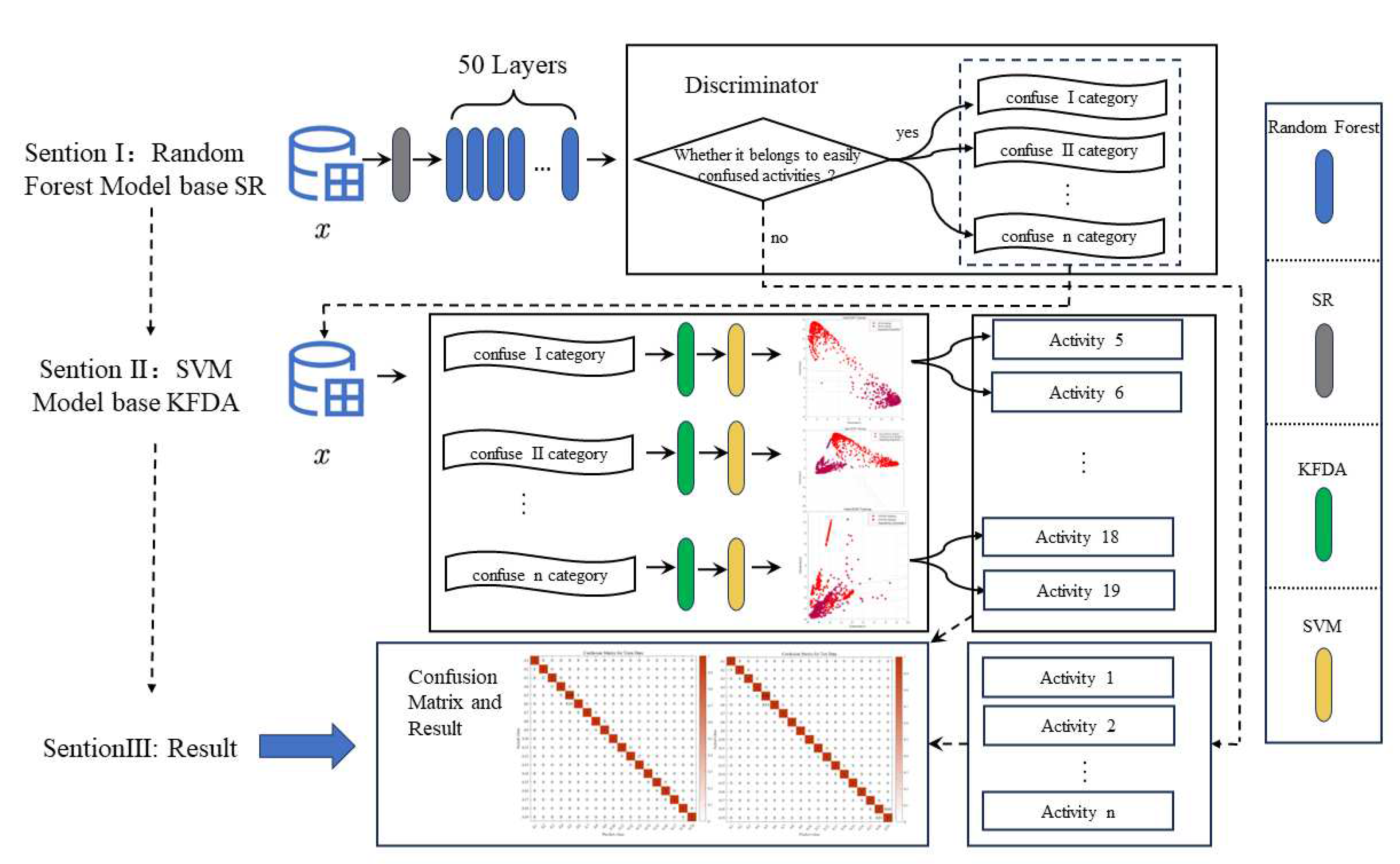
Figure 3.
Pre- and post-data pre-processed to correspond to 19 human activities.
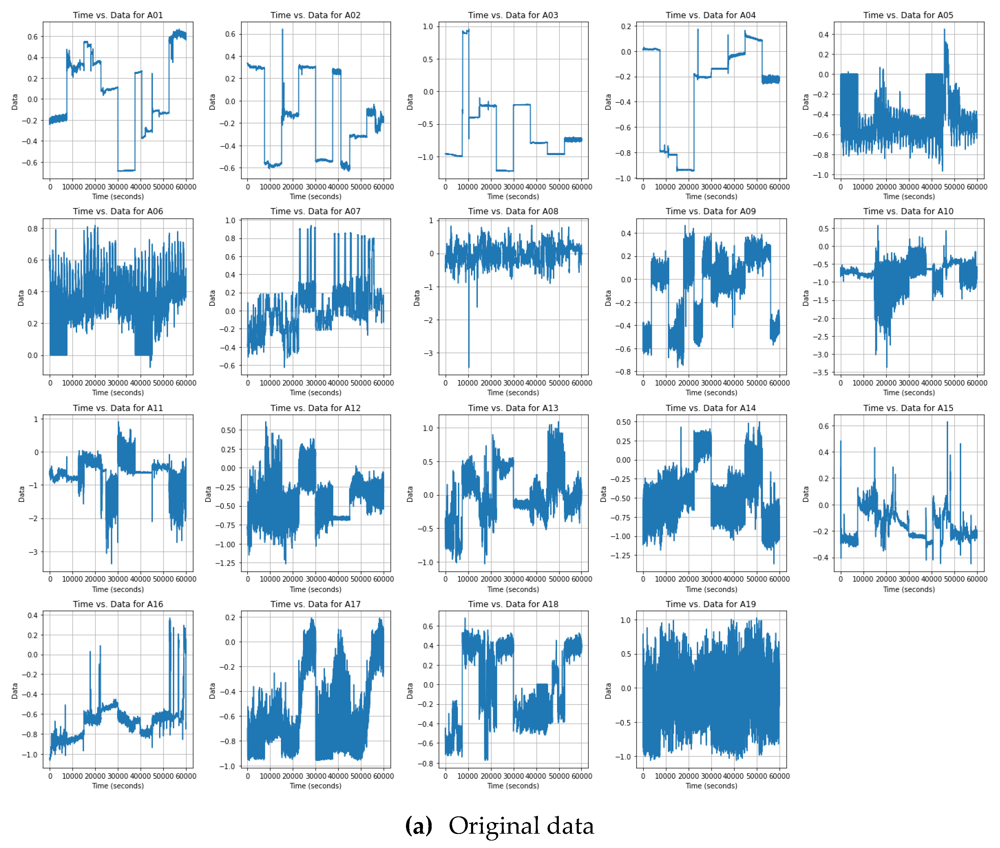
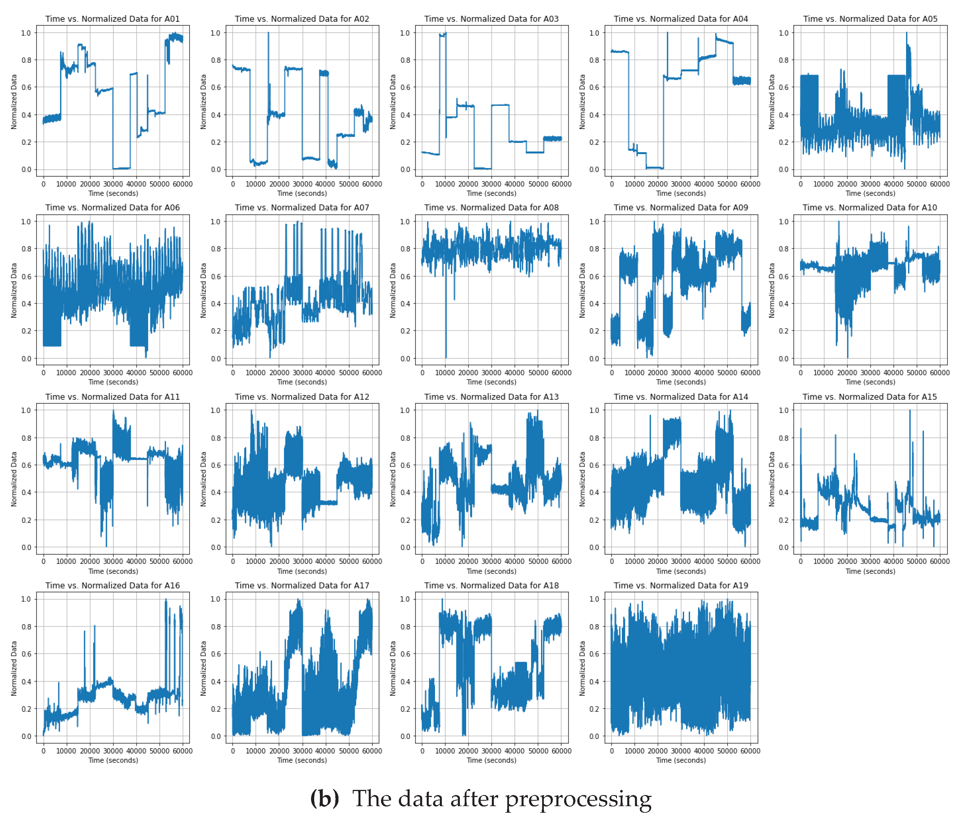
Figure 4.
Presentation of the Random Forest Model base on Stepwise regression algorithm Workflow.
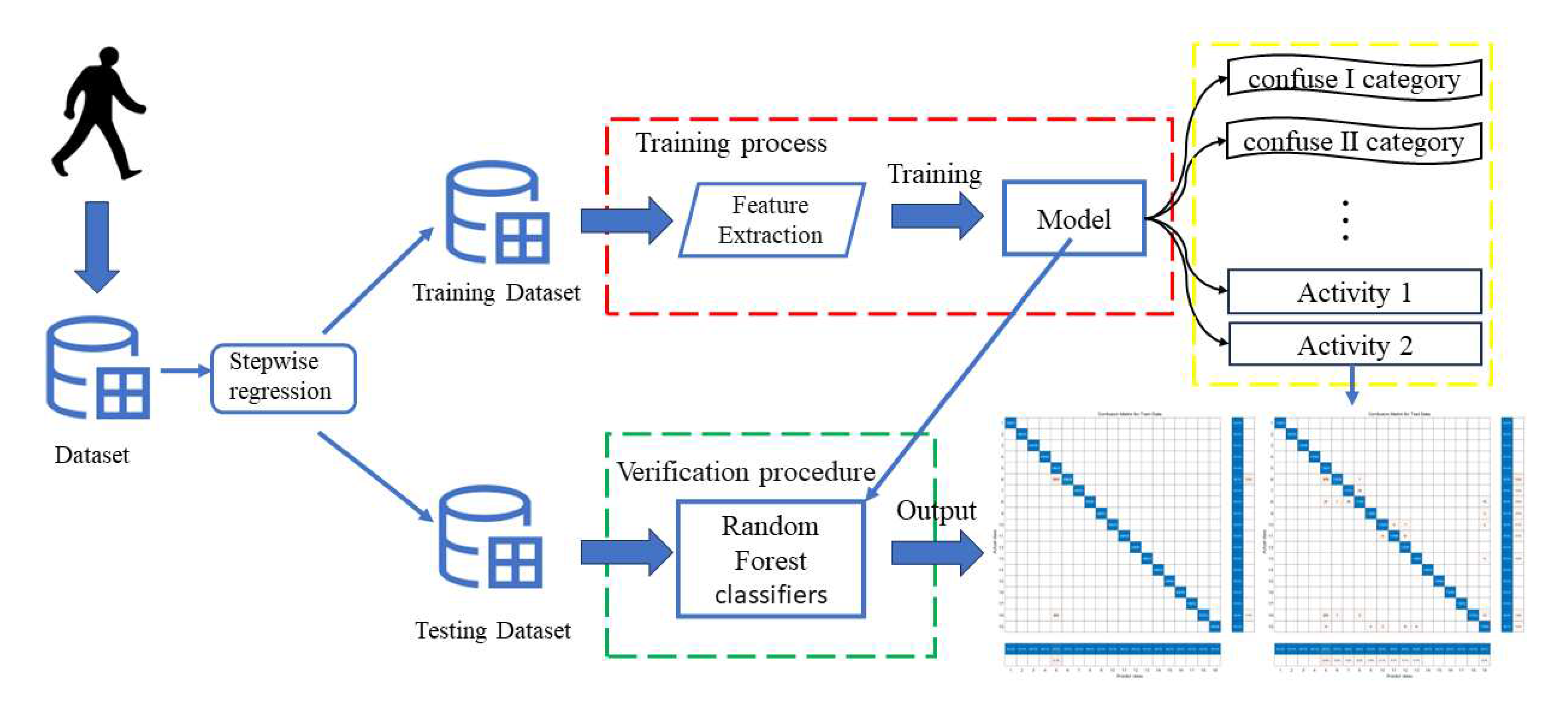
Figure 5.
Random forest algorithm flow chart.
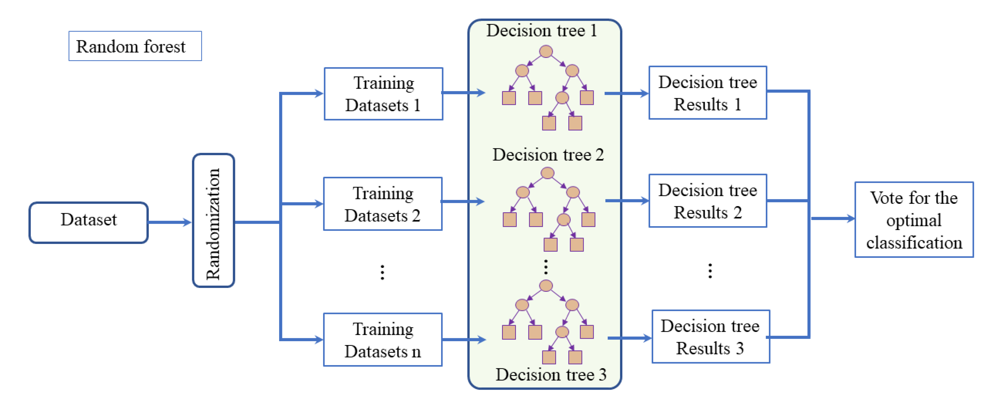
Figure 6.
SVM model workflow based on kernel Fisher discriminant analysis.
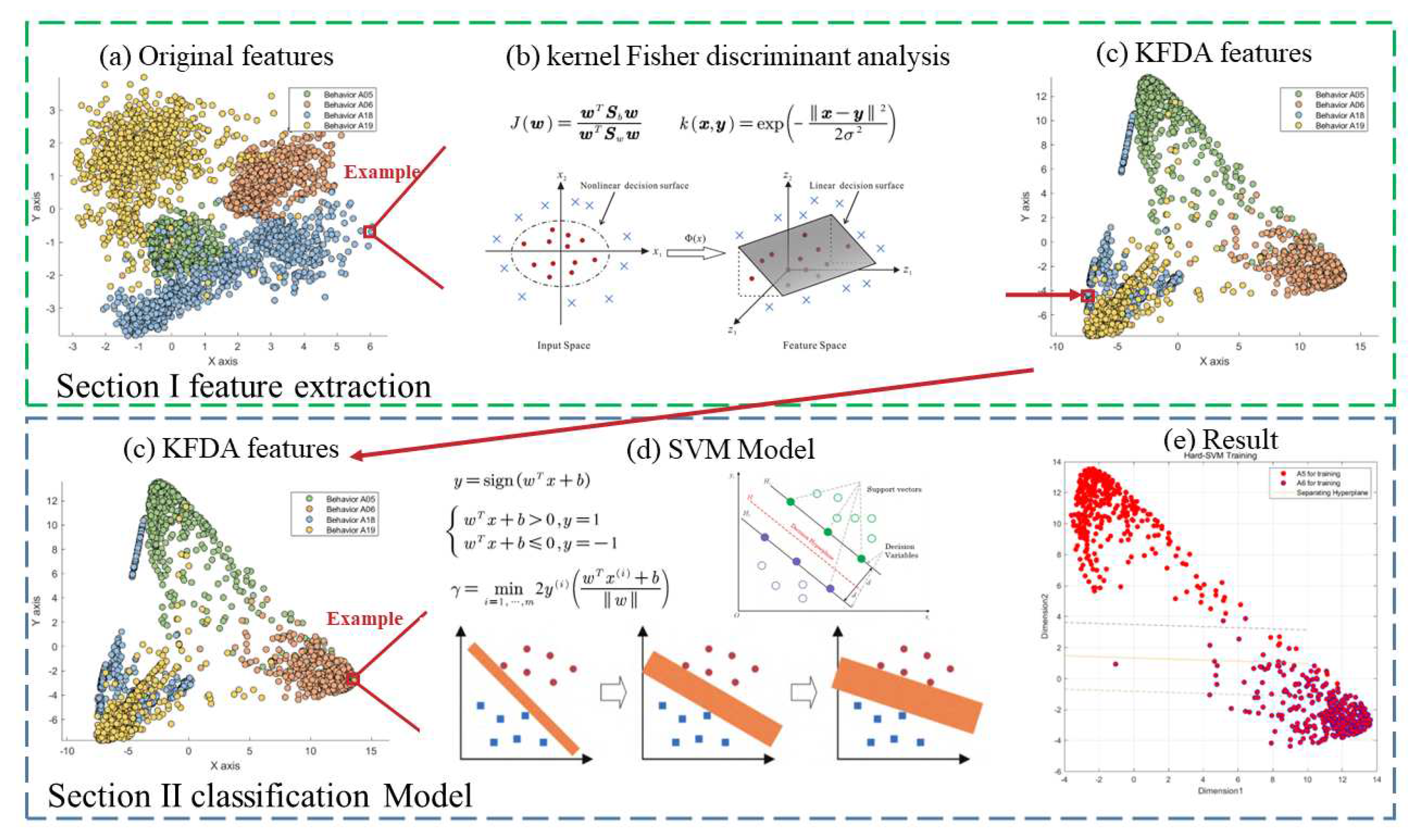
Figure 7.
Transformation process illustration of a KFD model. A nonlinear mapping function ϕ(x) converts a nonlinear problem in the original (low dimensional) input space to a linear problem in a (higher dimensional) feature space (from [43]).
Figure 7.
Transformation process illustration of a KFD model. A nonlinear mapping function ϕ(x) converts a nonlinear problem in the original (low dimensional) input space to a linear problem in a (higher dimensional) feature space (from [43]).
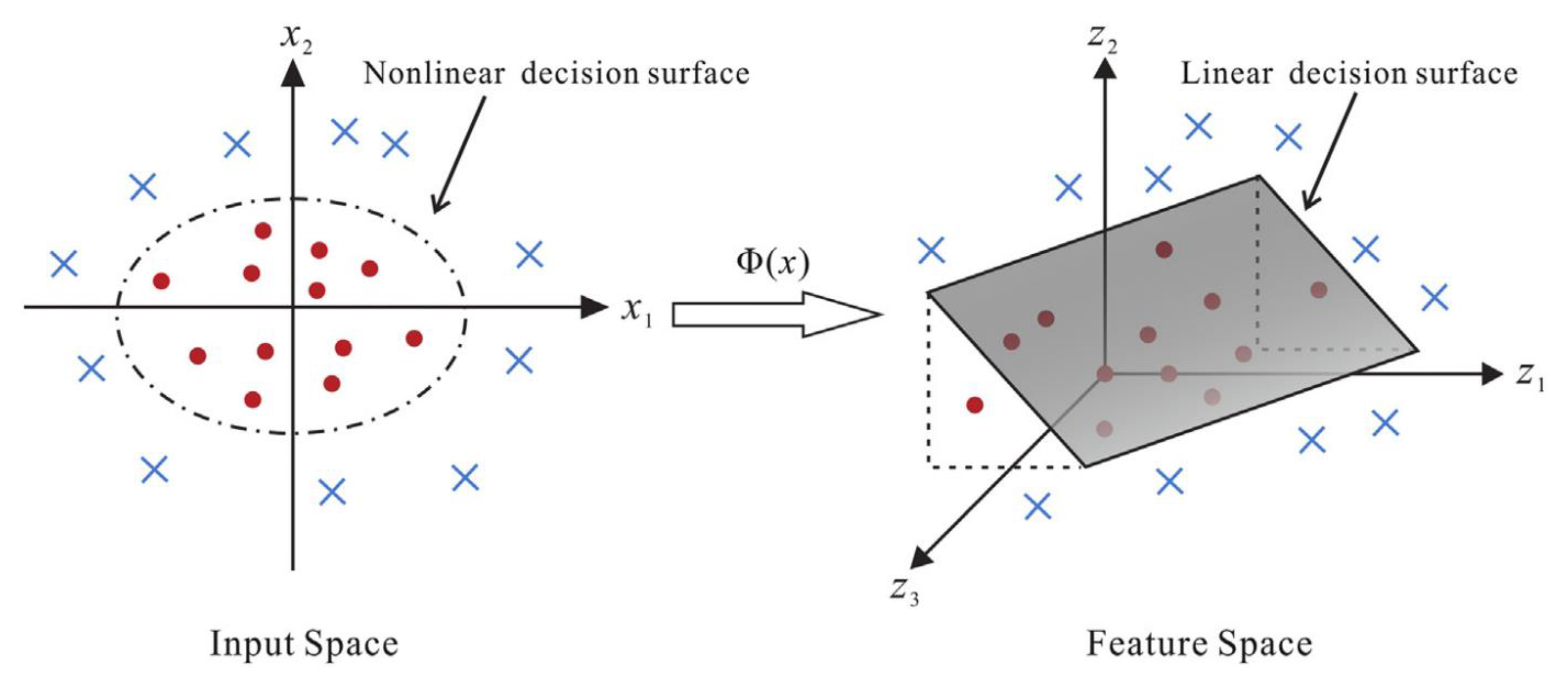
Figure 8.
Vector machine classification flow chart.
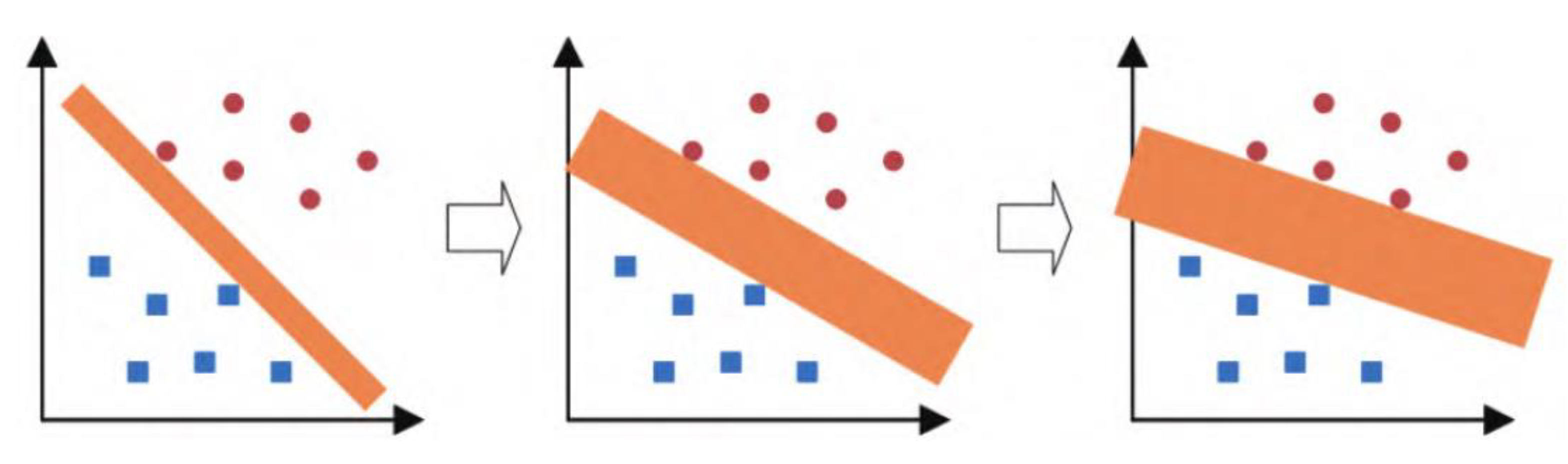
Figure 9.
Vector machine classification schematic.
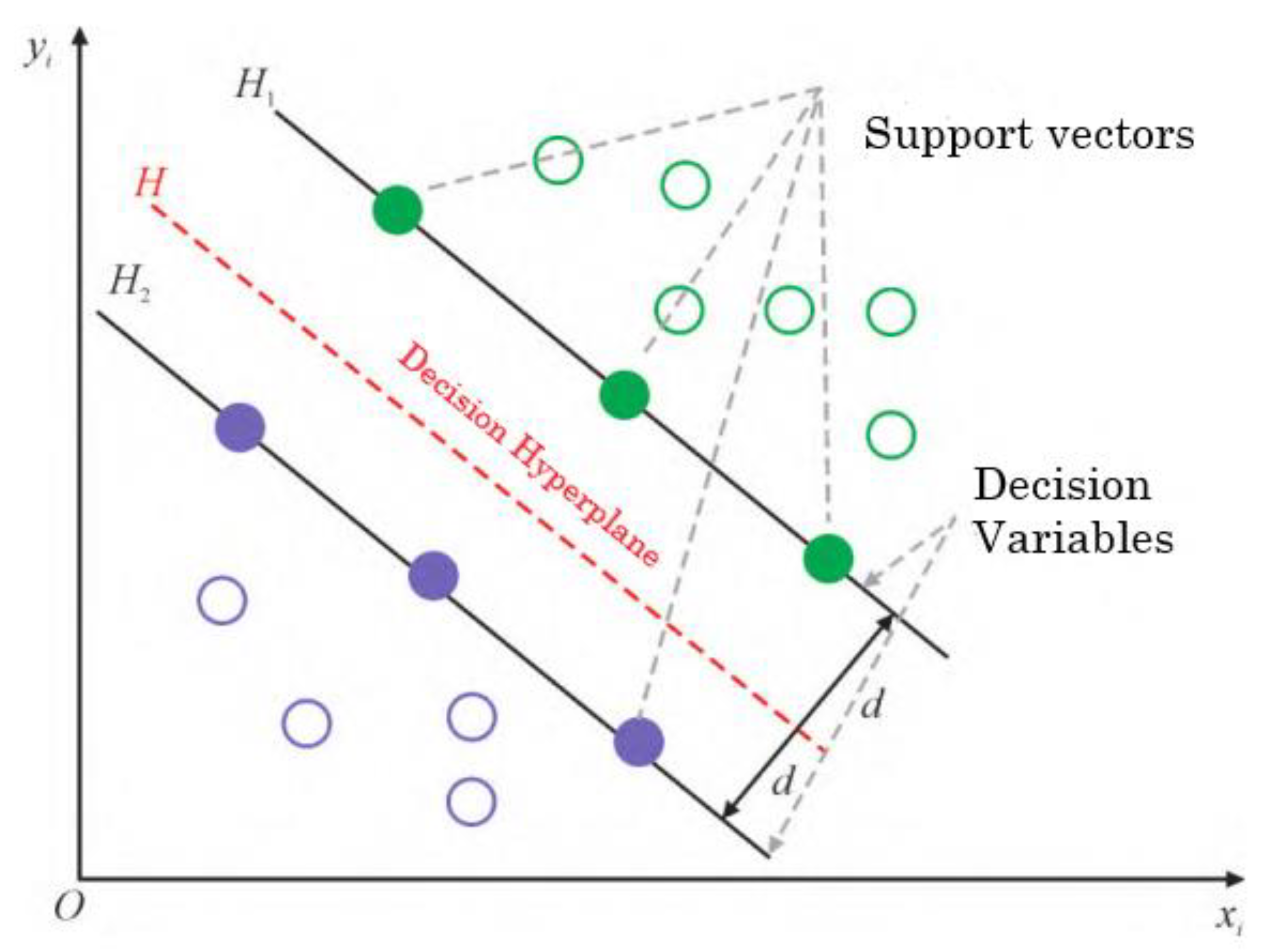
Figure 10.
Weights of important features chart.
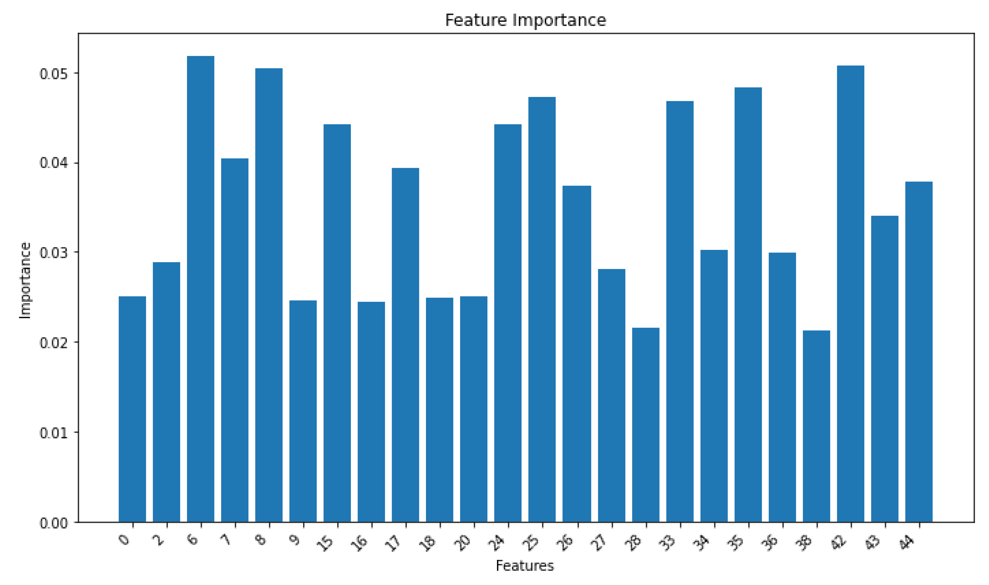
Figure 11.
Plot of the number of decisions versus error in the random forest model.
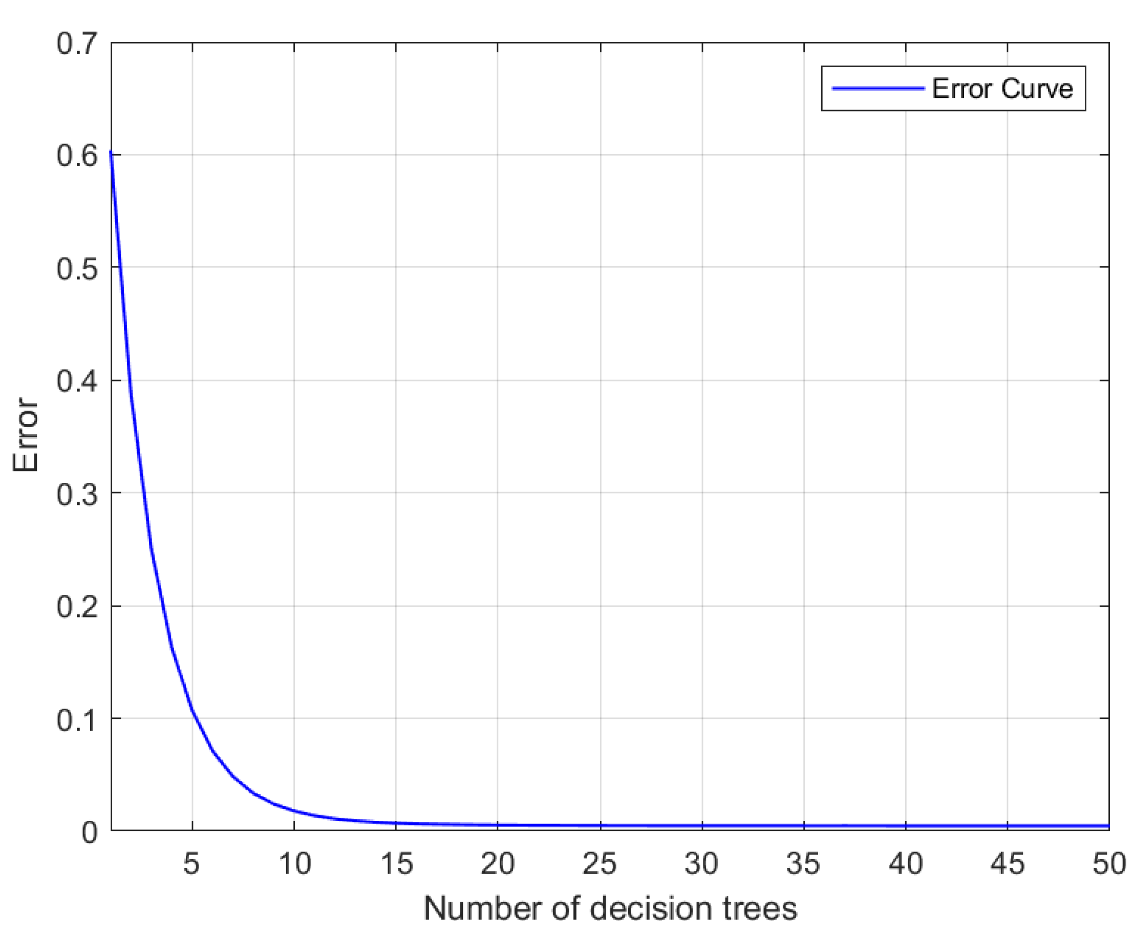
Figure 12.
Random forest model recognition results comparison chart.
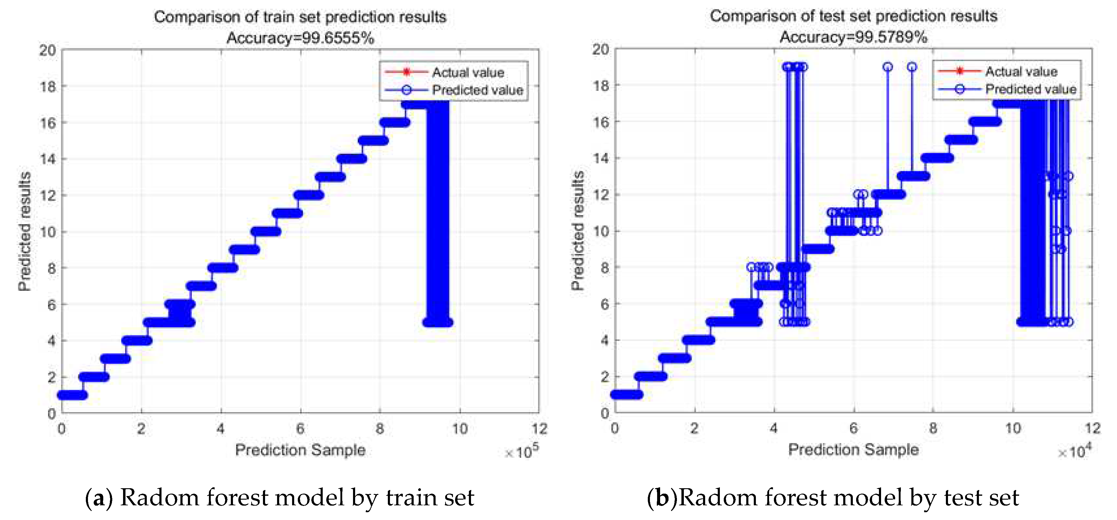
Figure 13.
Confusion matrix of test set and training set random forest training.
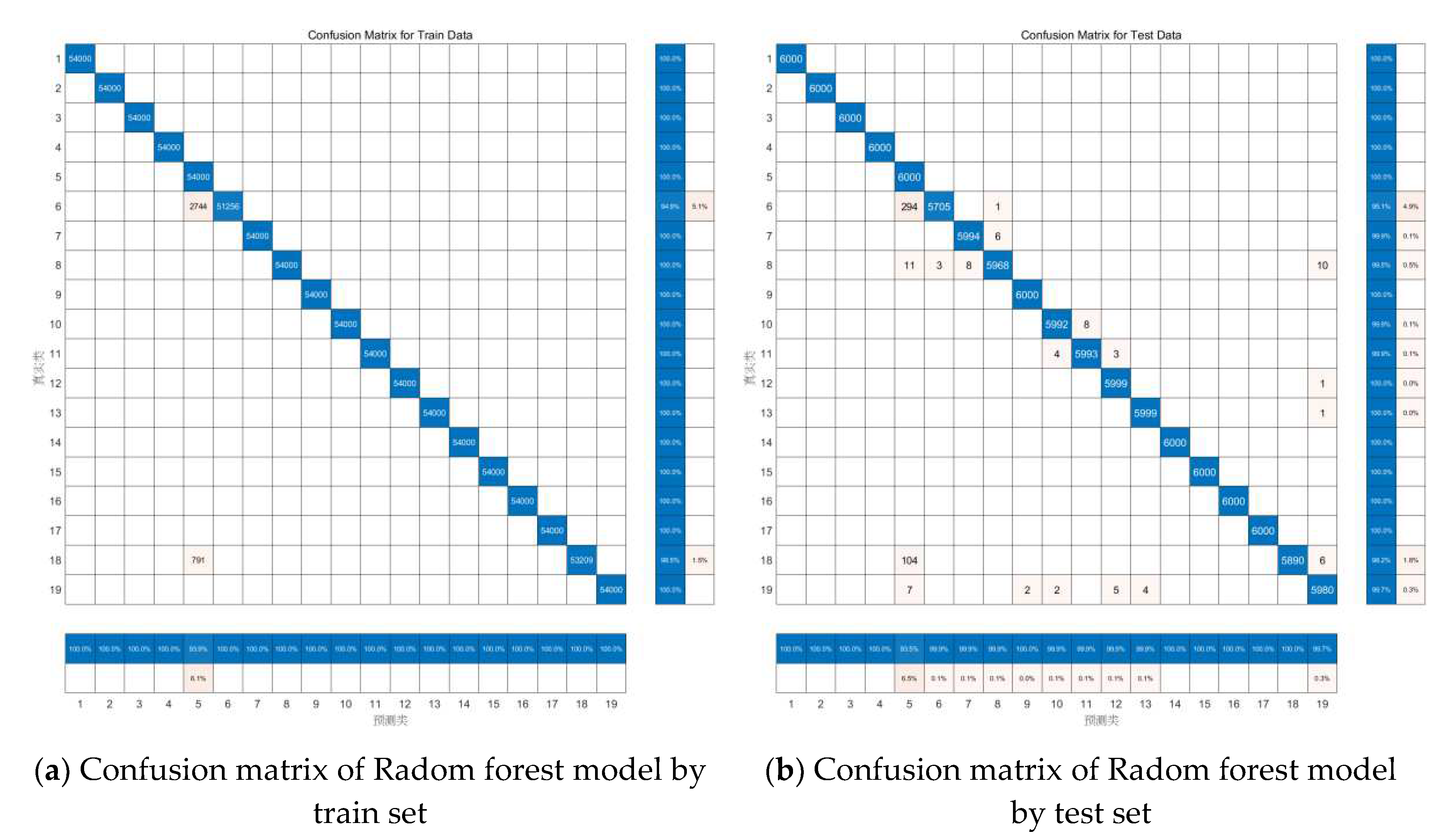
Figure 14.
primary feature and PCA feature.
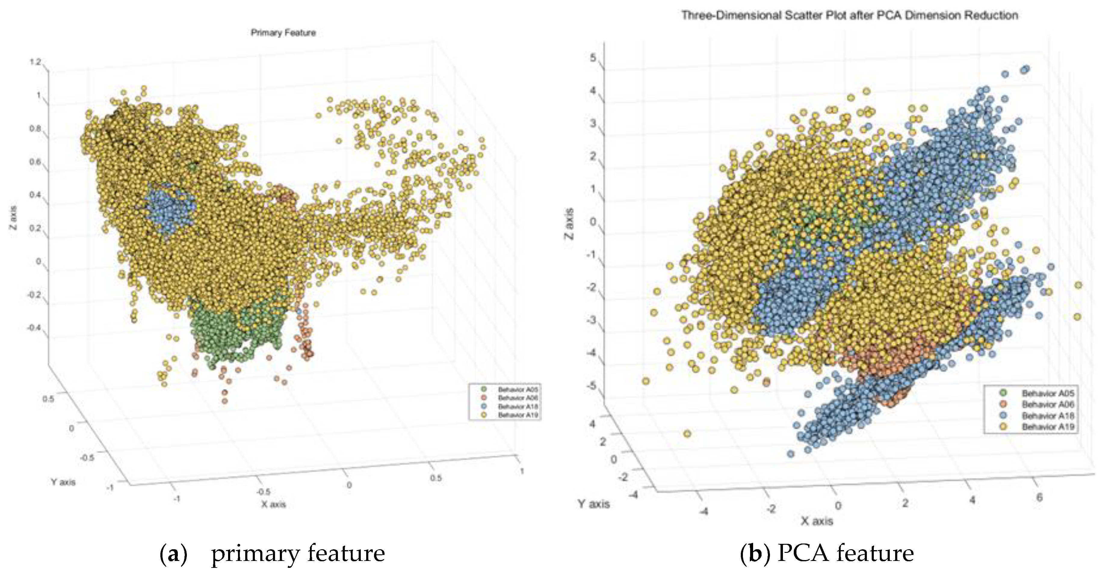
Figure 15.
The Result of Kernel Fisher Discriminant Analysis with varying parameter .
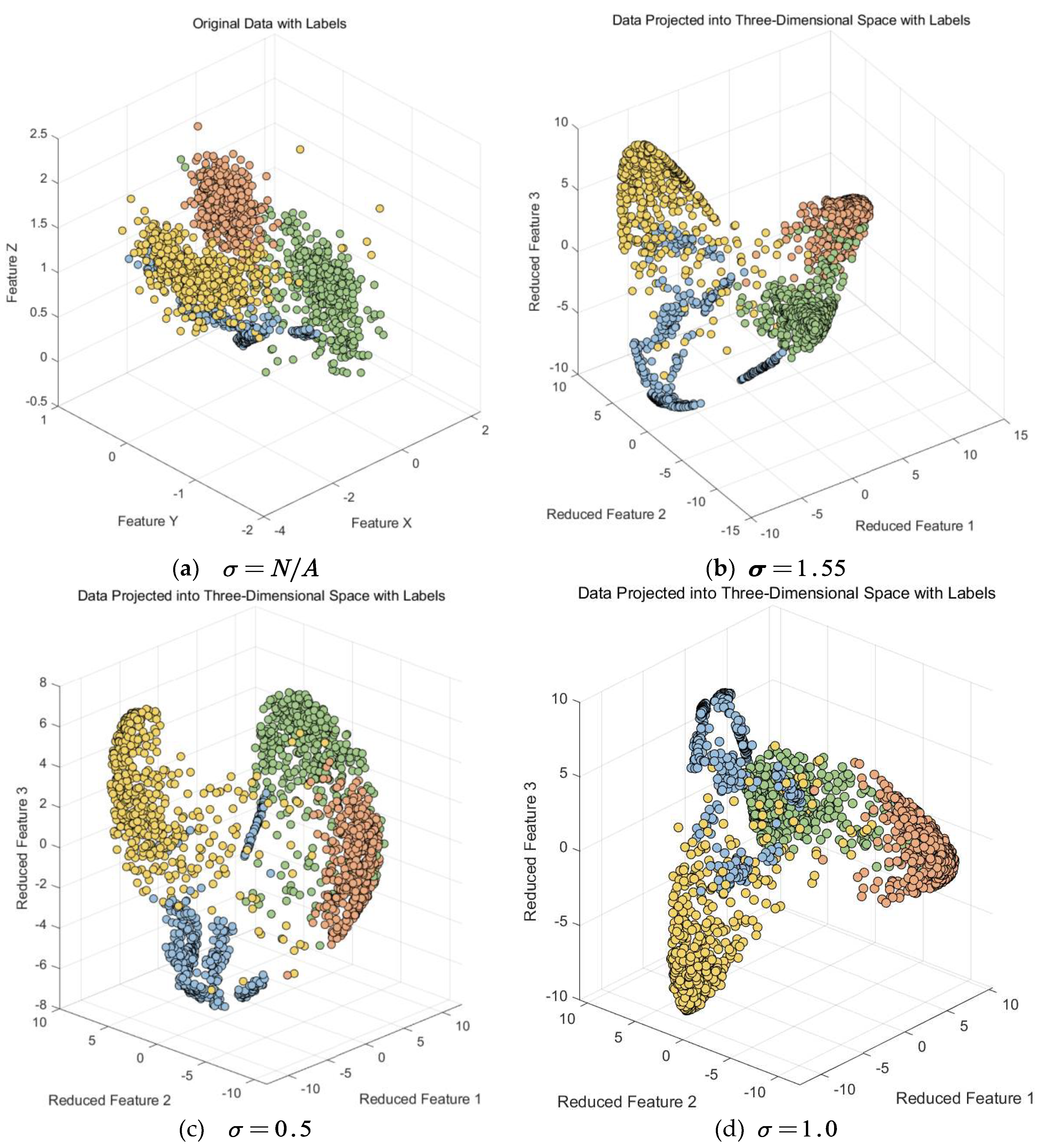
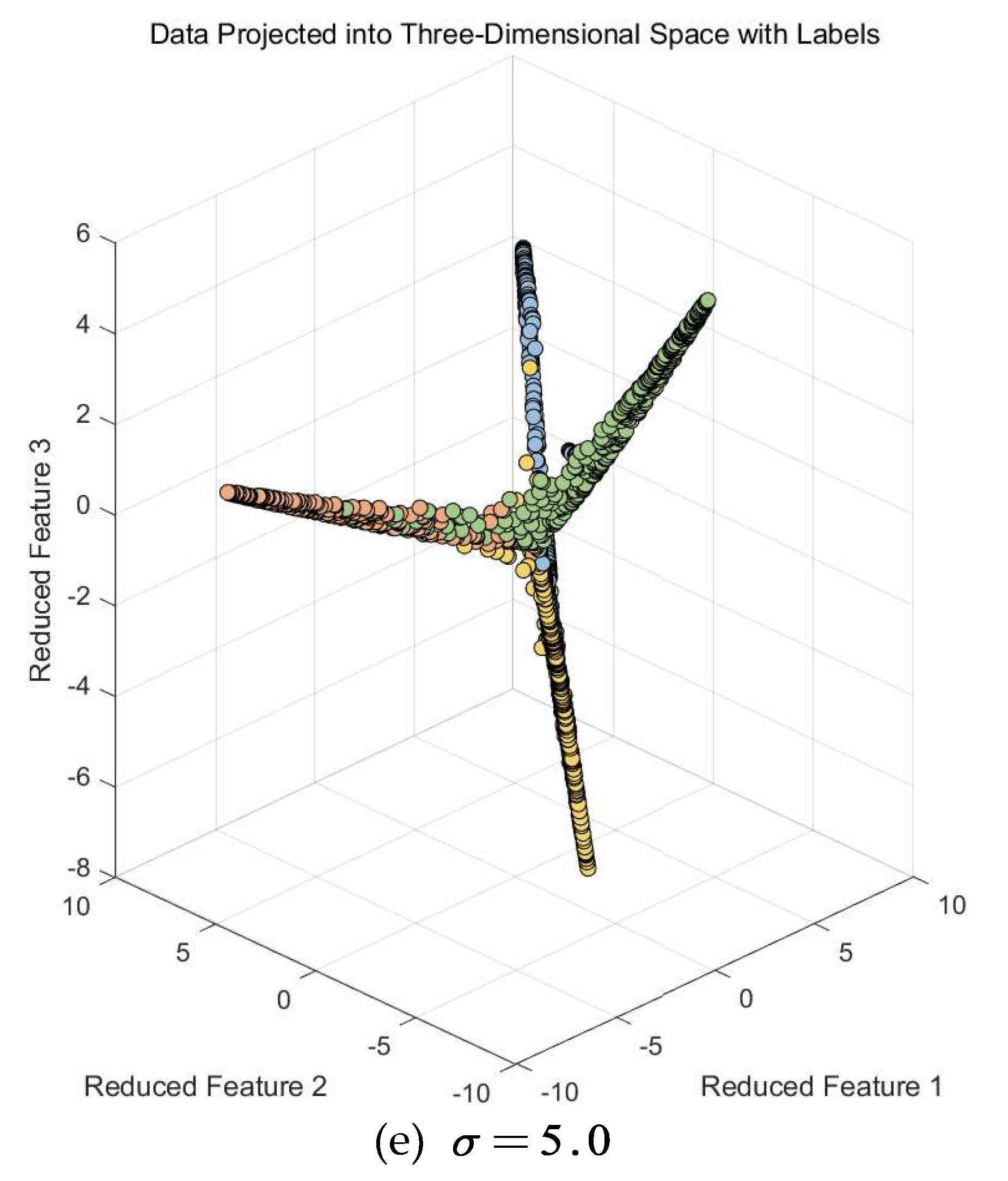
Figure 16.
kernel Fisher discriminant analysis feature.
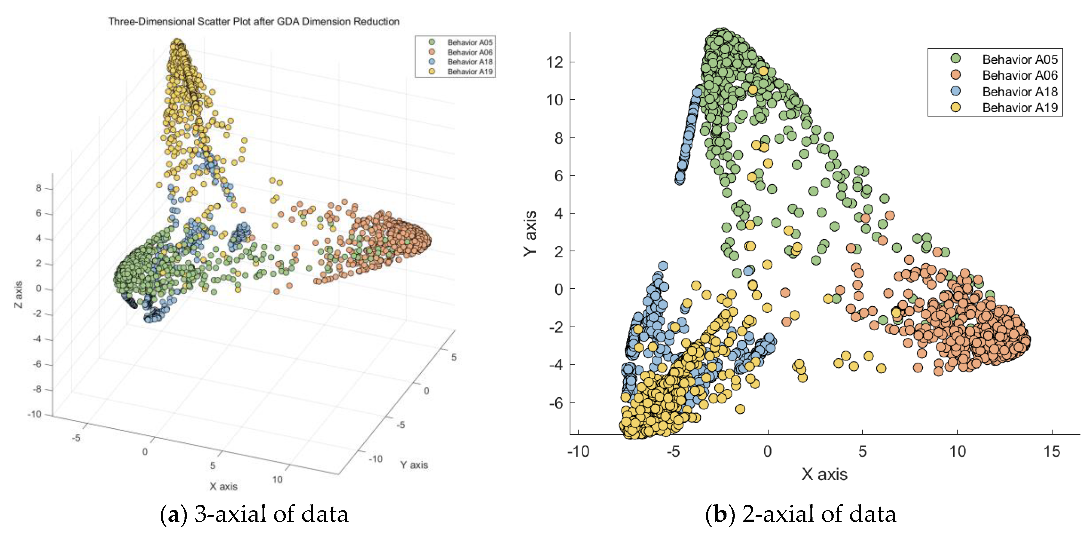
Figure 17.
SVM preliminary segmentation obfuscation I class result graph.
Figure 18.
SVM preliminary segmentation obfuscation I class result graph.
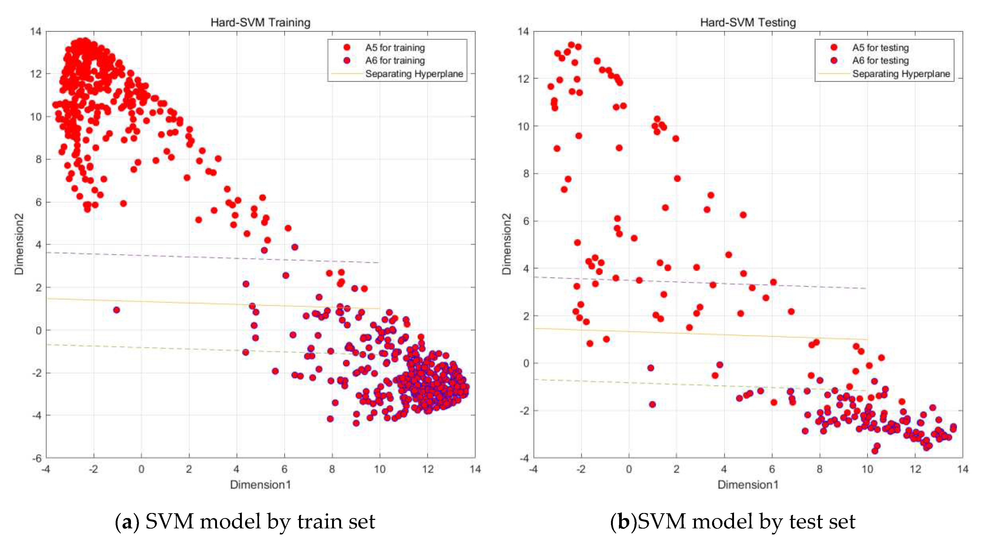
Figure 19.
SVM preliminary segmentation obfuscation I class result graph.
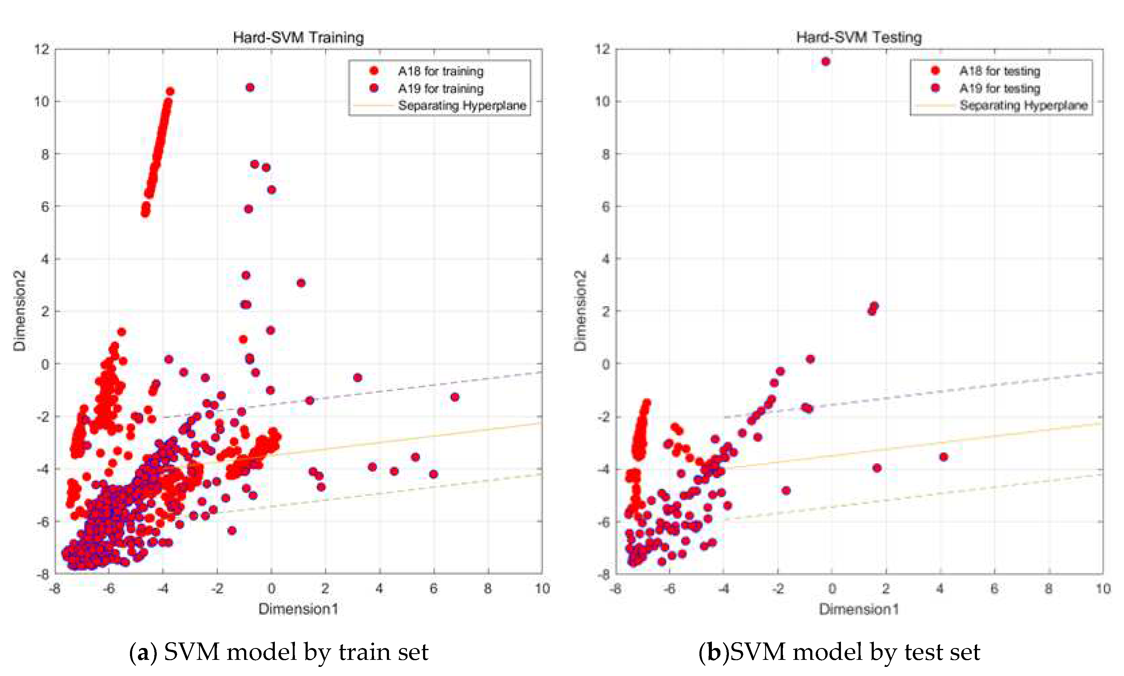
Figure 20.
Confusion matrix diagram for two-level classifier.
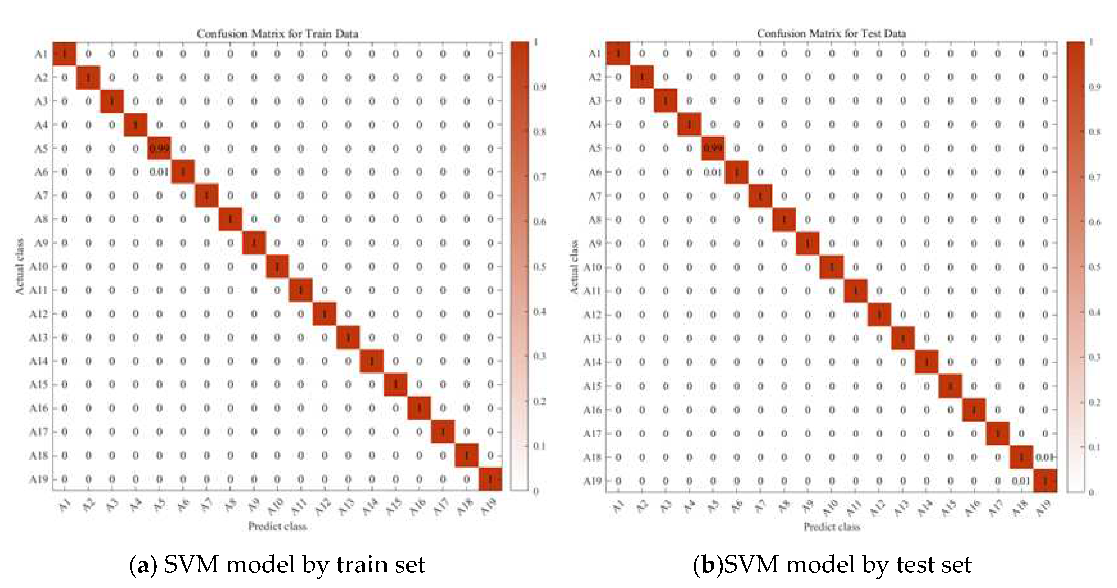
Figure 21.
Let k be the cross-validation result for 5.
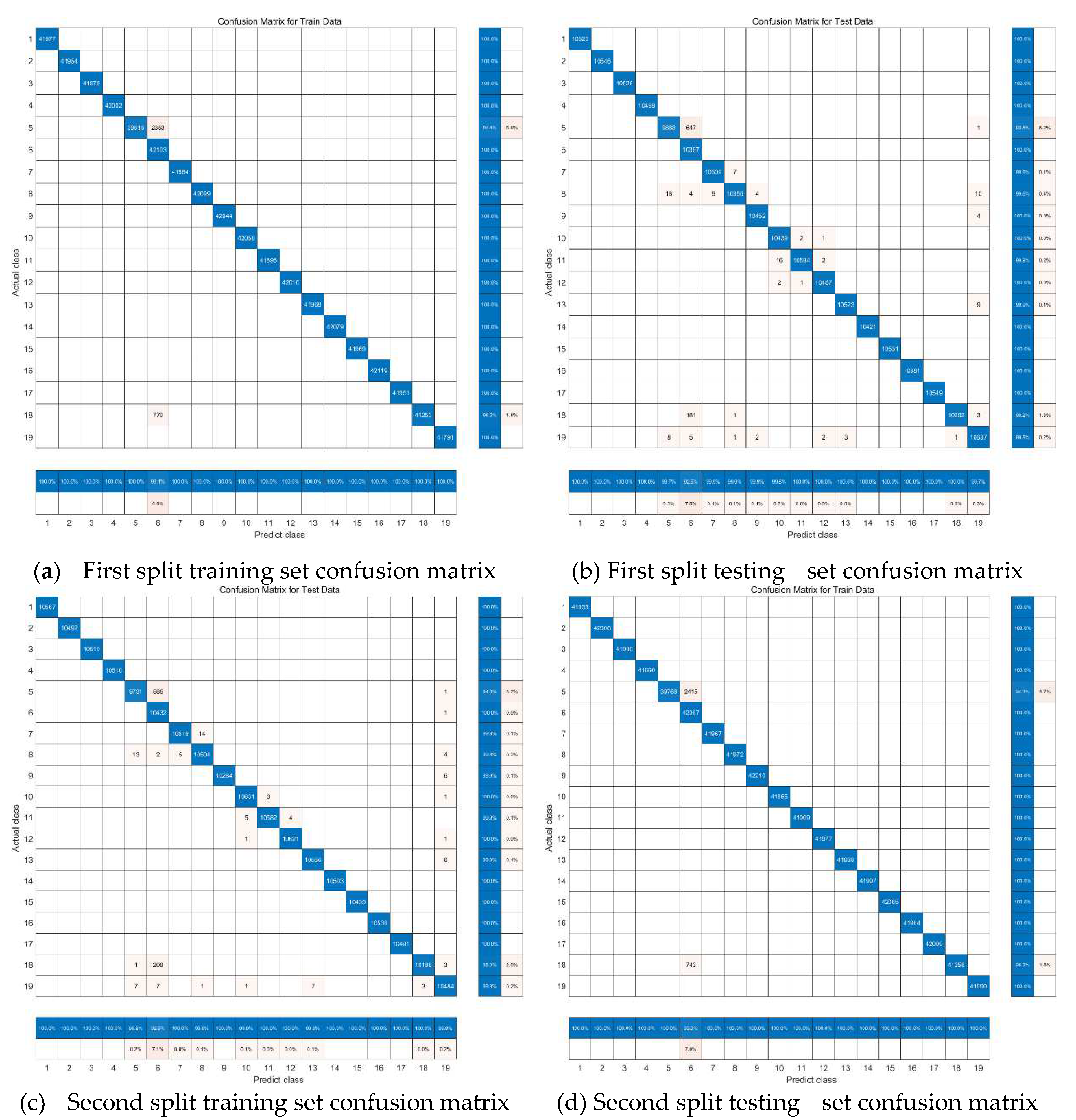
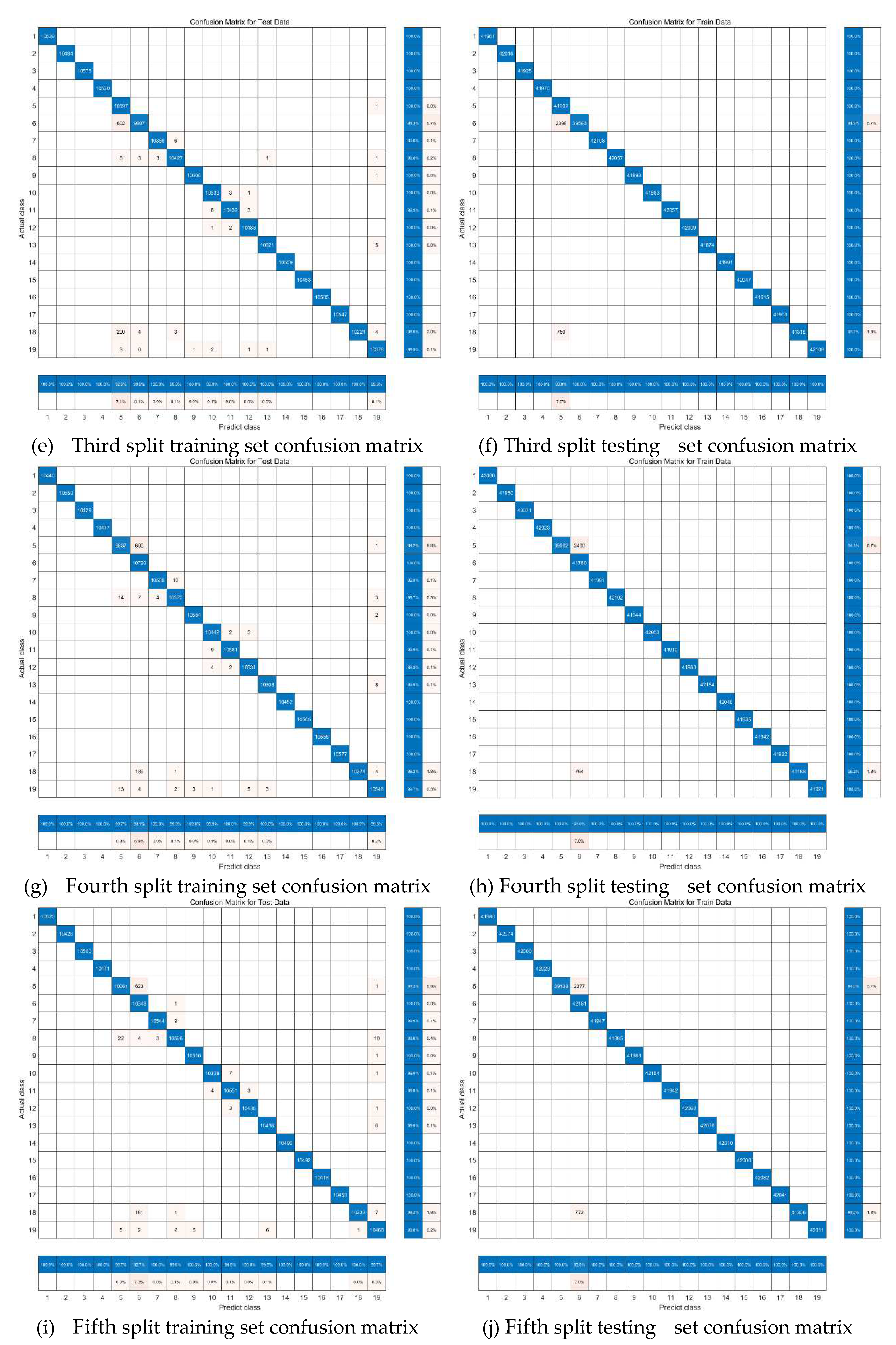
Figure 22.
SVM Model ROC Curve and AUC value.
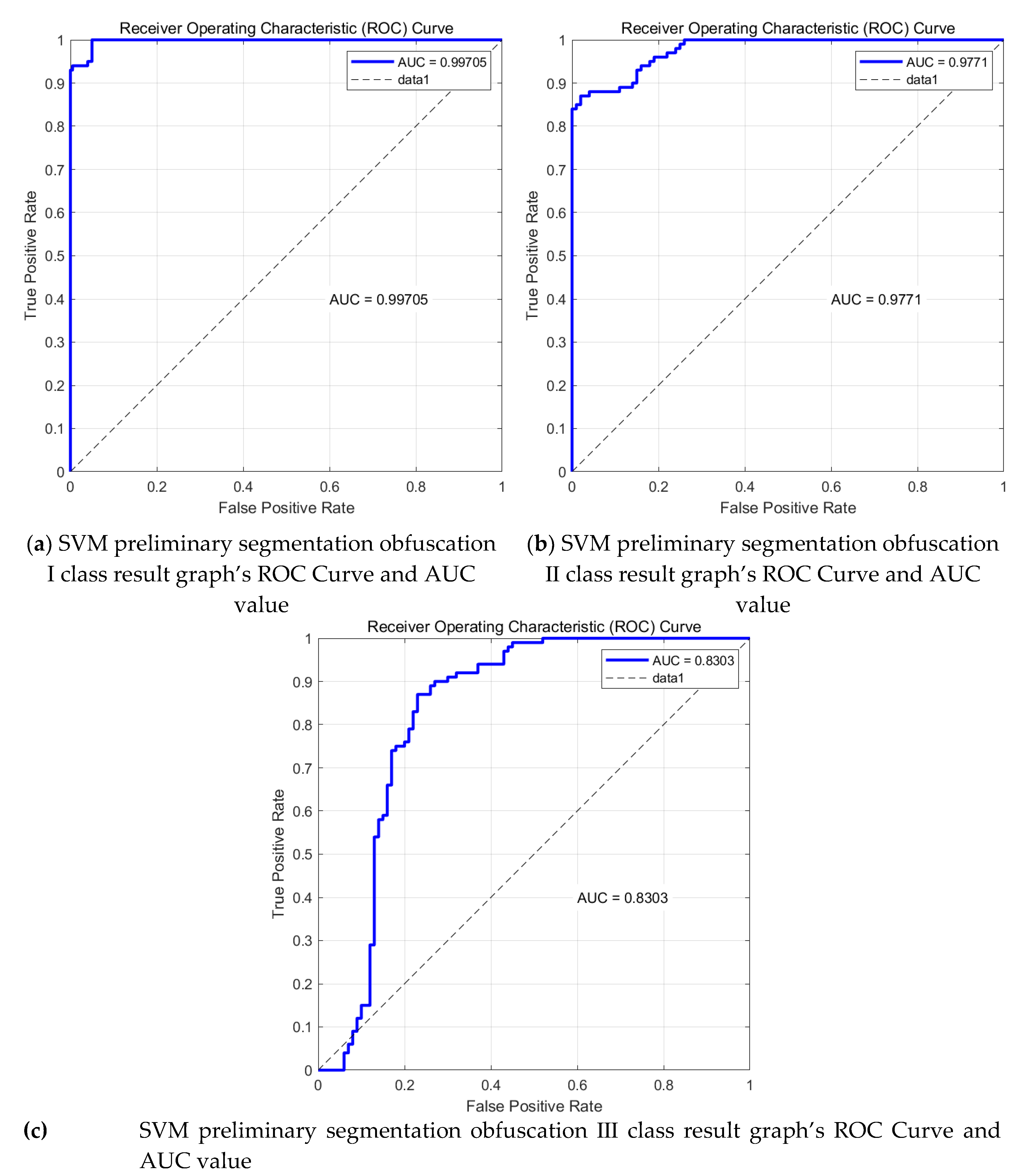

Table 1.
Comparison between datasets: UCI DSA,UCI HAR, WISDM and UCI ADL.
| UCI DSA | UCI HAR | WISDM | IM-WSHA | |
|---|---|---|---|---|
| Type of activity studied | Short-time | Short-time | Short-time | Short-time |
| Different volunteers | Yes | Yes | Yes | Yes |
| Volunteers Number | 4 | 30 | 36 | 10 |
| Fixed sensor frequency | Yes | Yes | Yes | Yes |
| Instances | 9120 | 10299 | 1098207 | 125955 |
| Sensors | Acc. and gyro. | Acc. and gyro. | Acc | Acc. and gyro. |
| Sensor data collection | Comprehensively | Comprehensively | Selectively | Selectively |
| Sensor type | Phone | Phone | Phone | IMU |
| Sensor number | 3 | 3 | 1 | 3 |
| Activities type | 19 | 6 | 6 | 11 |
Table 2.
Table of Specific Actions and Corresponding Codes in the Text.
| Behavior | Codes | Behavior | Codes |
|---|---|---|---|
| sitting | A1 | walking on a treadmill with a speed of 4 km/h (15 deg inclined positions) | A11 |
| standing | A2 | running on a treadmill with a speed of 8 km/h | A12 |
| lying on back | A3 | exercising on a stepper | A13 |
| lying on right side | A4 | exercising on a cross trainer | A14 |
| ascending stairs | A5 | cycling on an exercise bike in horizontal | A15 |
| descending stairs | A6 | cycling on an exercise bike in vertical positions | A16 |
| standing in an elevator still | A7 | rowing | A17 |
| moving around in an elevator | A8 | jumping | A18 |
| walking in a parking lot | A9 | playing basketball | A19 |
| walking on a treadmill with a speed of 4 km/h (in flat) | A10 |
Table 3.
Number of decisions and error rate.
| Number of decisions tree | Error rate |
|---|---|
| 1 | 63.1% |
| 5 | 10.5% |
| 10 | 2.8% |
| 20 | 1.2% |
| 35 | 0.8% |
| 50 | 0.3% |
Table 4.
This is a table. Tables should be placed in the main text near to the first time they are cited.
Table 4.
This is a table. Tables should be placed in the main text near to the first time they are cited.
| Ratio (training:testing) | UCI DSA | |
|---|---|---|
| Training data | Testing data | |
| 9:1 | 99.6555% | 99.5789% |
| 8:2 | 99.6043% | 99.5689% |
| 7:3 | 99.66% | 99.5269% |
| 6:4 | 99.6756% | 99.5445% |
| 5:5 | 99.6656% | 99.5040% |
| 4:6 | 99.6706% | 99.3753% |
Table 5.
Random forest Result table between datasets: UCI DSA,UCI HAR, WISDM and UCI ADL.
| Ratio (training:testing) | UCI DSA | WISDM | IM-WSHA | |||
|---|---|---|---|---|---|---|
| Training data | Testing data | Training data | Testing data | Training data | Testing data | |
| 9:1 | 99.6555% | 99.5789% | 99.9415% | 99.1819% | 99.9973% | 97.5342% |
| 8:2 | 99.6043% | 99.5689% | 99.9543% | 98.6841% | 99.9982% | 96.9773% |
| 7:3 | 99.66% | 99.5269% | 99.6646% | 98.5631% | 99.9977% | 96.8102% |
| 6:4 | 99.6756% | 99.5445% | 99.6326% | 98.4698% | 99.9973% | 96.4045% |
| 5:5 | 99.6656% | 99.5040% | 99.6061% | 98.3741% | 99.9984% | 95.9813% |
| 4:6 | 99.6706% | 99.3753% | 99.5841% | 98.2694% | 99.996% | 95.3001% |
Table 6.
Confusion action classification table.
| Confusion category | Easily confused actions |
|---|---|
| Confusion Ⅰ category | A5,A6,A18,A19 |
| Confusion Ⅱ category | A7,A8 |
Table 7.
Random forest Result table between datasets: UCI DSA,UCI HAR, WISDM and UCI ADL.
| Ratio (training:testing) | A5、A6 and A18、A19 Accuracy (%) | A5 and A6 Accuracy (%) | A18 and A19 Accuracy (%) | |||
|---|---|---|---|---|---|---|
| Training data | Testing data | Training data | Testing data | Training data | Testing data | |
| 9:1 | 99.90 | 99.75 | 95.11 | 90.98 | 78.10 | 66.77 |
| 8:2 | 98.96 | 98.41 | 95.12 | 90.56 | 81.00 | 78.75 |
| 7:3 | 96.56 | 95.83 | 95.28 | 91.04 | 75.33 | 74.70 |
| 6:4 | 95.75 | 95.06 | 95.33 | 91.25 | 68.25 | 69.30 |
| 5:5 | 94.90 | 95.35 | 94.80 | 90.65 | 73.20 | 64.80 |
| 4:6 | 93.91 | 94.62 | 90.56 | 85.34 | 77.16 | 70.65 |
Table 8.
Comparison of recognition accuracy of the proposed method with other state-of-the-art methods over UCI DSA, UCI HAR, WISDM and IM-WSHA datasets.
Table 8.
Comparison of recognition accuracy of the proposed method with other state-of-the-art methods over UCI DSA, UCI HAR, WISDM and IM-WSHA datasets.
| Method | UCI DSA | UCI HAR | WISDM | IM-WSHA |
|---|---|---|---|---|
| MS-DLD[25] | 88.3%[25] | |||
| HPAR[26] | 91.83%[26] | 90.18%[26] | ||
| HDAR[27] | 91.45%[27] | |||
| RPLB[28] | 83.18%[28] | |||
| Kinematics features withkernel sliding perceptron[29] | 81.47%[29] | |||
| Estimation algorithm[30] | 80.49[30] | |||
| Accelerometer and Gyroscope Sensors[31] | 96.33%[31] | |||
| Deep CNN-LSTM[32] | 93.11%[32] | |||
| Deep CNN-GRU[33] | 96.20%[33] | 97.21%[33] | ||
| EdgeHARNet[34] | 94.036%[34] | |||
| MarNASNet-b[35] | 94.20%[35] | 90.62%[35] | ||
| DMEFAM[36] | 96%[36] | 97.9%[36] | ||
| BLSTM[37] | 98.37%[37] | 99.01%[37] | ||
| CAEL-HAR[38] | 96.45%[38] | 98.57%[38] | ||
| 2D CNN-LSTM[49] | 92.95%[49] | |||
| MVTS[50] | 98.96%[50] | |||
| SR-KS | 99.71% | 98.71% | 99.12% | 97.6% |
Disclaimer/Publisher’s Note: The statements, opinions and data contained in all publications are solely those of the individual author(s) and contributor(s) and not of MDPI and/or the editor(s). MDPI and/or the editor(s) disclaim responsibility for any injury to people or property resulting from any ideas, methods, instructions or products referred to in the content. |
© 2023 by the authors. Licensee MDPI, Basel, Switzerland. This article is an open access article distributed under the terms and conditions of the Creative Commons Attribution (CC BY) license (http://creativecommons.org/licenses/by/4.0/).
Copyright: This open access article is published under a Creative Commons CC BY 4.0 license, which permit the free download, distribution, and reuse, provided that the author and preprint are cited in any reuse.


