Submitted:
18 October 2023
Posted:
19 October 2023
Read the latest preprint version here
Abstract
Soybean yield prediction is a challenging problem in plant breeding that is often affected by many different factors simultaneously. Hyperspectral reflectance data from plants and soil data provide breeders with useful information about soybean plant health and using these different types of data to predict yield is an active area of research. Furthermore, breeding programs encounter challenges such as data imbalance and external factors like genotype variability across different environments, which present significant hurdles in the development of yield prediction models for large-scale breeding programs. In this work, we perform a comprehensive study of predicting yield using both hyperspectral reflectance and soil data to understand what scenario's offer the best chances of predicting yield with high accuracy. We demonstrate a cluster based ensemble approach for yield prediction using hyperspectral reflectance data that can perform well for large scale breeding programs by efficiently harnessing useful information from data through an unsupervised approach.
Keywords:
ML:Ensemble methods
; ML: applications
1. Introduction
Plant breeders strive to select superior genetic lines to meet the needs of farmers, industry, and consumers, with seed yield as among the essential traits under selection in row crops [1]. Traditional methods of estimating seed yield consist of machine harvesting plots at the end of the growing season and using these data to make decisions to select or discard in breeding programs. Variety development is resource-intensive, and several thousand plots are harvested each year. With time and resource constraints, this process can be quite draining on a program. To overcome these challenges, plant breeders and scientists have proposed new methods of assessing lines by using the power of remote sensing combined with machine learning to predict yield in season and to reduce the time and labor requirements at harvest [2,3,4,5,6,7,8].
Accurate in-season yield prediction is difficult due to the complexity of the differences in genotype, variability in macro and micro environments, and other factors that can be difficult to measure and quantify across the growing season. Hyperspectral reflectance data can capture plant vegetation indices not observable in the visible light spectrum [9] and in-season seed yield prediction with rank performance [10]. Hyperspectral data and vegetation indices have a large number of predictors, and typically few observed data points due to the complexity of the data. Machine learning (ML) is a valuable tool for dealing with these complex and often nonlinear prediction problems [11,12]. However, this is an evolving field, and continual improvement is desired to achieve high success in yield prediction for improved decision-making by breeders.
Recently proposed cyber-agricultural system (CAS) leverages advances in continual sensing, artificial intelligence, intelligent actuators in breeding and production agriculture [13]. Phenotyping is an integral part of CAS and utilizes advanced imaging techniques and computational methods to ease data collection and analysis, offering advances in yield prediction [14]. Several approaches have focused on high-throughput phenotyping using drones in the study of crop yield prediction of various crops like cotton, maize, soybean, and wheat [15]. In addition to 2-dimensional data from drones, research has shown the utility of canopy fingerprints to uniquely characterize the three-dimensional structure of soybean canopies through point cloud data [16]. However, there remains room for improvement in developing models that integrate multiple types of data, particularly soil characteristics and hyperspectral reflectance, for a more comprehensive understanding of soybean yield. The physical and chemical properties of soil influence the availability of essential nutrients, which directly affect plant growth and development and have great potential to be used to increase yield prediction model accuracy.
Deep learning models have demonstrated significant potential in various fields, i.e., finance [17], and have become increasingly prevalent. However, they often require large amounts of data, which may not always be accessible. When data is limited, shallow machine learning models may be more appropriate than deep models. However, selecting the proper shallow model for the task is critical to ensuring accurate results. Ensemble learning effectively structures shallow models, particularly when data is insufficient for deep models or is prone to overfitting.
Ensemble learning is a powerful ML concept that works by constructing a set of individual models and then combining the output of all the constructed models using a decision fusion strategy to produce a single answer for a given problem. The two main challenges of ensemble learning are: (1) how to select appropriate training data and learning algorithms to make the individual learning tasks as diverse as possible, and (2) how to finalize the learning results by proper fusion of the individual learning tasks [18]. Ensemble learning considers the effects of individual learning tasks to provide an efficient solution to the main problem. Since large-scale breeding programs are affected by experimental plot design, ensemble learning can help develop efficient prediction algorithms that can factor in the effect of the plot design to provide yield prediction for large-scale scenarios.
Motivated by these objectives, we propose two ensemble approaches that effectively incorporate potential experimental design effects into the modeling paradigm. The first approach, the field ensemble model, leverages the experimental design information from the breeding program to make predictions. The second method, the cluster ensemble approach, utilizes unsupervised learning techniques to uncover underlying patterns within the dataset and subsequently constructs an ensemble strategy based on this derived information. Additionally, we assess various Machine Learning architectures that solely utilize Spectral or Soil data for yield prediction.
2. Materials and Methods
2.1. Description of Data
Soil, hyperspectral reflectance, and seed yield data were collected across two years (2020 and 2021) in preliminary yield trials (PYT), and the advanced yield trials (AYT), with each having multiple locations per year in Iowa. PYT were established as row column designs with a plot width of 1.52m and a plot length of 2.13m with a 0.91m alleyway between plots in each row. AYT were also established with a row column design with a plot width of 1.52m, a plot length of 5.18m and a 0.91m alleyway between each plot in each row. Details of data collection and processing are given below.
2.1.1. Soil Data
Digital soil mapping for ten soil features was conducted in addition to the collection of hyperspectral data. Soil cores were collected using a 25m grid sampling pattern, with samples taken to a depth of 15cm using a soil probe. Digital soil mapping using the cubist regression ML algorithm described in Khaledian and Miller [19] was used to generate digital soil maps with a 3mx3m pixel size. Each plot boundary was defined using a polygon shape file, and the mean soil feature value for each plot was extracted. Soil features were smoothed by taking a 3x3 moving mean of each plot, and using this mean value as the soil feature value for further analysis. Smoothing the soil features using a 3x3 moving mean helps to reduce noise and variability in the data, providing a more representative value for further analysis and interpretation. The following soil features were collected: Calcium(CA), Cation Exchange Capacity(CEC), Potasium(K), Magnesium(Mg), Organic Matter(OM), Phosphorous(P1), Percent Hydrogen(Ph), Clay, Sand, and Silt.
- MM_CA: Calcium content in a particular plot.
- MM_CEC: Cation capacity exchange in a particular plot.
- MM_K: Potasium content in a particular plot.
- MM_MG: Magnesium content in a particular plot.
- MM_OM: Organic matter content in a particular plot.
- MM_P1: Phosporous content in a particular plot.
- MM_PH: PH level in a particular plot.
- MM_CLAY: Clay content in a particular plot.
- MM_SAND: Sand content in a particular plot.
- MM_SILT: Silt content in a particular plot.
2.1.2. Hyperspectral Reflectance Data
Hyperspectral reflectance was collected for each plot using a Thorlabs CCS200 spectrometer (Newton, NJ) using a system similar to that described in Bai et al. [20]. Each plot had spectral data collected at three timepoints (T1, T2, T3) each year, covering 200 nm to 1000 nm wavelegnths (see Figure 1). We report on the third timepoint (T3) because these measurements have the highest feature importance values based on preliminary unreported data analysis, and as measurements get closer to physiological maturity there is a greater relationship between reflectance data and yield. This division was performed to test the ensemble approaches described in Section 3, as it was based on preliminary unreported data analysis that indicated higher feature importance values for the measurements taken at the third timepoint, and a stronger relationship between reflectance data and yield as the measurements approached physiological maturity.
Using the hyperspectral reflectance values we computed fifty-two vegetation indices taken from Li et al. [2] details of which are given in Table A1 in Appendix A. The number of data points in each of the four fields are given in Table 1.
2.1.3. Yield Data
Plot level seed yield data was collected for each plot with an Almaco small plot combine (Nevada, IA), and was adjusted to 13% moisture and converted to Kg/ha. Data was collected in blocks based on the layout of the breeding program, which grouped lines based on similar genetic backgrounds and their maturity groups.
Before computing the vegetation-indices we performed preprocessing on the data to remove unwanted and outlier data points from our analysis. The steps taken for preprocessing are as follows:
- All observations for band values less than 400 nm were removed. This was done since we noticed many anomalies in the readings in those bands.
- All datapoints which had negative hyperspectral values in any of the bands ranging from 400 nm to 1000 nm were removed.
- All datapoints which had negative seed yield values were removed.
3. Methodology
In this section we discuss the methodologies used for modelling end season yield with vegetation indices and soil data. We first describe the methodologies for modelling vegetation indices followed by soil data.
3.1. Yield Prediction Using Vegetation Indices
In order to determine the most effective method of modeling end-season yield using vegetation indices, we conducted an analysis using a range of shallow models. Our approach involved evaluating the performance of these models based on their ability to capture the relationship between end-season yield and the fifty-two vegetation indices. This allowed us to identify the most suitable model for accurately modeling this relationship.
Once we were able to identify the best model we then wanted to explore whether we can determine a smaller subset of vegetation indices which can predict yield with same/increased accuracy as that of the 52 original chosen indices. For this we used a backward sequential feature selector algorithm implemented using MLXtend package [21] in python. The algorithm was implemented using subsets of several sizes to determine the smallest subset that still provided high accuracy.
3.2. Ensemble Models Using Vegetation Indices
Even though we can find a suitable model and an optimum set of vegetation indices for our dataset an important question to consider while developing models for our problem is whether the shallow model proving best for our chosen vegetation indices would also be able to perform well in cases when the number of datapoints is significantly large. Often for big datasets shallow models can overfit resulting in noisy predictions. Ensemble learning can prove very efficient in these scenarios since it allows diving a data into smaller subsections and then ensembling results from appropriate models fitted to each of those subsections. But an important question here is how should one determine the appropriate subsections such that the ensemble results prove to be most efficient. Two plausible choices are (a) manual grouping based on the nature of data collection/experimentation or (b) unsupervised data driven groups without considering any aspect of data collection/experimentation.
In this study, we explore two different ensemble approaches. The first approach, known as the field-weighted ensemble model and second approach, referred to as the cluster-based ensemble model. Each of these approaches is described below:
3.2.1. Field Weighted Ensemble Model
The ensemble framework described in this section aims to leverage the expert information on data collection to group data on plot level seed yield and vegetation indices. For our analysis the collected plot level seed yield data and the vegetation-indices computed for those same plots was grouped from all the experiments within each test (PYT and AYT) for each year (2020 and 2021) to divide the data into four subsections, hereon referred to as fields. The number of datapoints in each field is given in Table 1.
Our proposed modelling paradigm fits separate models to each of the four fields and then combine predictions from each of the four tasks to arrive at the final prediction. The steps to build the field ensemble framework are given below
- Let denote the dataset for the kth field (dataset for kth task), where denotes the predictors (vegetation indices) and the response (seed yield), . Divide into and , where and denote the training and test set for respectively.
- Fit a random forest regression model [22] to every .
- Let , where for every data point in denote a new dataset. Here denotes the field membership of . Combine row wise to create a combined dataset .
- Fit a multinomial logistic regression classifier [23] on . This classifer provides the ensemble weights for new observations.
Now, let denote the dataset obtained by combining , row wise.. Then for any datapoint from , let denote the prediction obtained from the kth task. Let denote the classification weights for obtained using the multinomial classifier, where is the probability that belongs to (). The final prediction of is then obtained as
3.2.2. Cluster Ensemble Model
The cluster ensemble method uses a unsupervised approach to find clusters in the data that serve as datasets for the indivitual tasks. The appeal of this method is that it does not require any additional informtaion to create appropriate subsections of the data like the field-weighted ensemble model, but is able to determine the subsections from the original dataset using an unsupervised learning approach. The steps to build the cluster ensemble framework are given below:
Let be a dataset where are the predictors (vegetation indices) and is the response (seed yield). In this setting we do not assume any field information about . The aim here is to first identify possible clusters within , and then use the obtained cluster information to build our ensemble approach for prediction. For this setup we split the data into train and test parts namely and
- Divide into K homogeneous groups using k-means [24] and elbow method. Let be a variable denoting the cluster memberships of .
- Based on divide into K groups , . is hence the dataset for the kth task.
- Fit a random forest regression model to every , .
- Fit a logistic regression classifier to to determine the ensemble weights.
Now for any observation from let denote the prediction from the kth task, . Let be the ensemble weights for obtained using the classifier where is the probability that the belongs to the kth group . Then the final predicted value for is obtained as
A pictorial representation of both field-weighted ensemble approach and cluster ensemble approach is given in Figure 2.
Choice of model for individual tasks: Choice of the appropriate model for each individual task is an important aspect of both the approaches. We fitted several models for each task. These included linear regression, Ridge regression and Gaussian Process, but random forest regression yielded the best accuracy in terms of R-squared.
Our framework was implemented using the python library scikit-learn [25]
3.3. Yield Prediction Using Soil Data
Our analysis of the relationship between soil data and end-season yield follows a similar approach to that used for vegetation indices. Specifically, we began by identifying the optimal model for capturing the relationship between these two variables. We then used a backward sequential feature selection method to determine the most important soil factors for predicting end-season yield. By employing this approach, we were able to identify the key soil factors that are most strongly associated with end-season yield, and thus gain a deeper understanding of the factors that influence end season yield.
Our final step in this study was combining the best features from both vegetation indices and soil data to investigate if combining both modalities can improve the prediction accuracy significantly.
4. Results and Discussion
4.1. Hyperspectral Reflectance Data
4.1.1. Analysis Using Derived Vegetation Indices
In order to accurately predict end-season yield using vegetation indices derived from hyperspectral data, we conducted a rigorous analysis involving the fitting of multiple models to the data. Our objective was to identify the model that yielded the highest prediction accuracy. To achieve this, we employed an eighty-twenty train-test split and a 3-fold cross-validation approach to fit the various models. Table 2 indicates that random forest gives the highest accuracy for predicting end season yield. The actual vs predicted plot using random forest for vegetation data is given in Figure 4a
In order to determine the smallest subset of vegetation indices which can provide better/same performance accuracy we used backward sequential feature selection with random forest with subsets of different sizes to determine the smallest subset. The results of feature selection are given in Table 3. It is clearly evident that a subset of ten vegetation indices can provide accuracy similar to fifty two vegetation indices. The ten indices chosen by feature selection are MCARI, MCARI3, MTCI, ND1, NDchl, NDVI1, PVR, RVSI, SR1 and TCARI. Now note that the hyperspectal wavelengths needed to compute the choosen ten indices are 430 nm, 531 nm, 550 nm, 650 nm, 670 nm, 680 nm, 700 nm, 710 nm, 715 nm, 718 nm, 750 nm and 925 nm. This signifies that for end season soybean yield prediction it is only needed to collect data on twelve wavelengths rather than six hundred wavelengths.
Using the subset of ten vegatation indices we developed and tested our ensemble models details of which are as follows
4.1.2. Ensemble Models
In this section we compare the accuracy of the two approaches, and discuss the usefulness of the cluster ensemble approach for large scale scenarios and potential use in variety development.
4.1.3. Field Weighted Ensemble Model
For this experiment we performed an eighty-twenty train-test split on each of the four fields. Each individual task was fitted using a 3-fold cross validation and an eighty-twenty train-test split. To ensure we have fitted a good classifier to our combined training data, we used an eighty-twenty train-test split and a 3-fold cross validation on our combined data ( denoted by under Section 3.2.1). Our fitted classifier achieved an of 0.96 indicating that our fitted classifier will be able to generate appropriate ensemble weights for the weighted average prediction
The accuracy of each of the four tasks and the ensemble model for the combined test data are given in Table 4. It is evident that the individual field models do not achieve a good accuracy, with R-squared values ranging from -0.19 to 0.09. The field ensemble model is able to achieve a higher accuracy than all of the individual fields. This is because the ensemble weights are able to leverage the contributions of the four individual models for every test data to give an increase in accuracy. Although the increase in this case is not significant, this example is a clear indication that ensembling using the classification weights tends to provide better prediction. The main reason behind this low accuracy of the overall framework is because each of the individual fields have a poor fit, and that is mainly because of the low amount of data in each of the fields. We hypothesize that where fields have a sufficient amount of data to provide a good fit the ensemble can result in increased accuracy, and will be future research direction.
4.1.4. Cluster Ensemble Model
The first step in implementing the cluster ensemble model is creation of data for the individual tasks, i.e. clustering the predictors in our training set. Figure 3 shows the values of the sum of squared distances for k (number of clusters) values one to ten. The elbow plot suggest the optimum number of groups in the combined data to be two.

Table 5.
Number of observations in each of the clusters obtained by k-means on the training data.
| Cluster No. | Number of observations |
| 1 | 2100 |
| 2 | 428 |
To train our classifier and cluster ensemble model we use the same principle as Section 4.1.3. The obtained test accuracy for the classifier is 0.95. In each of the obtained clusters we fitted a random forest regression using a 3-fold cross validation. The test accuracy of the individual models and the task ensemble model are given in Table 6.
Figure 3.
Sum of squared distances for k values 1-9.
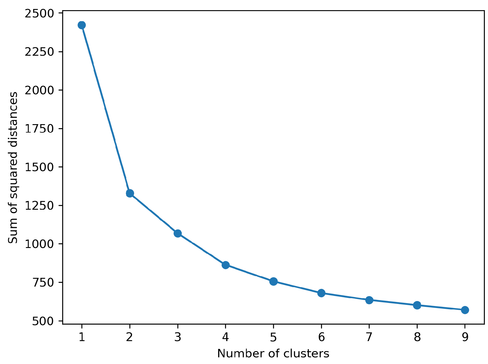
Figure 4.
From left to right: (a) The actual vs predicted plot for random forest on vegetation indices data (b) The actual vs predicted plot for random forest on soil data.
Figure 4.
From left to right: (a) The actual vs predicted plot for random forest on vegetation indices data (b) The actual vs predicted plot for random forest on soil data.
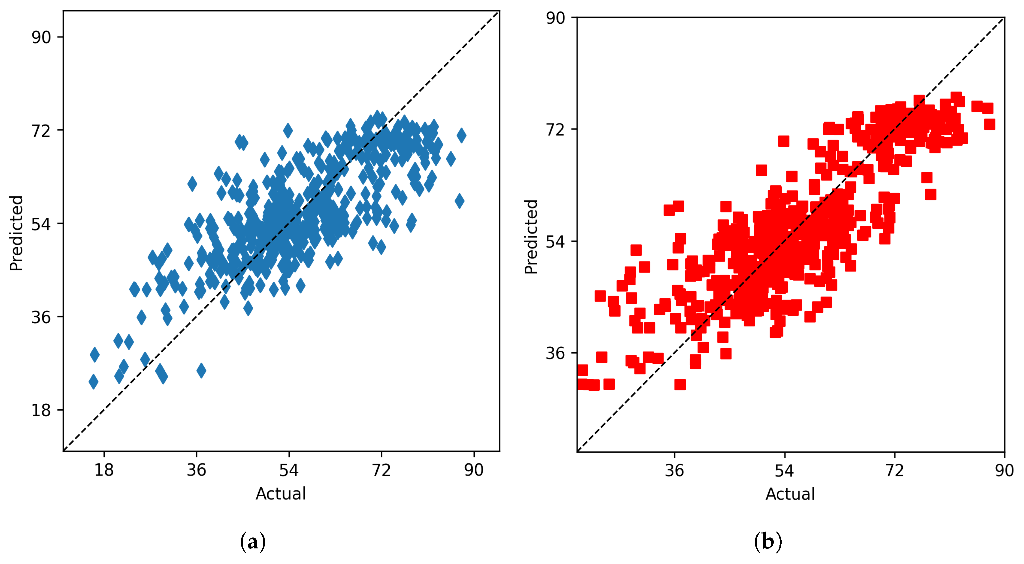
Figure 5.
From left to right: (a) The actual vs predicted plot for field-weighted ensemble model, (b) The actual vs predicted plot for cluster ensemble model.
Figure 5.
From left to right: (a) The actual vs predicted plot for field-weighted ensemble model, (b) The actual vs predicted plot for cluster ensemble model.
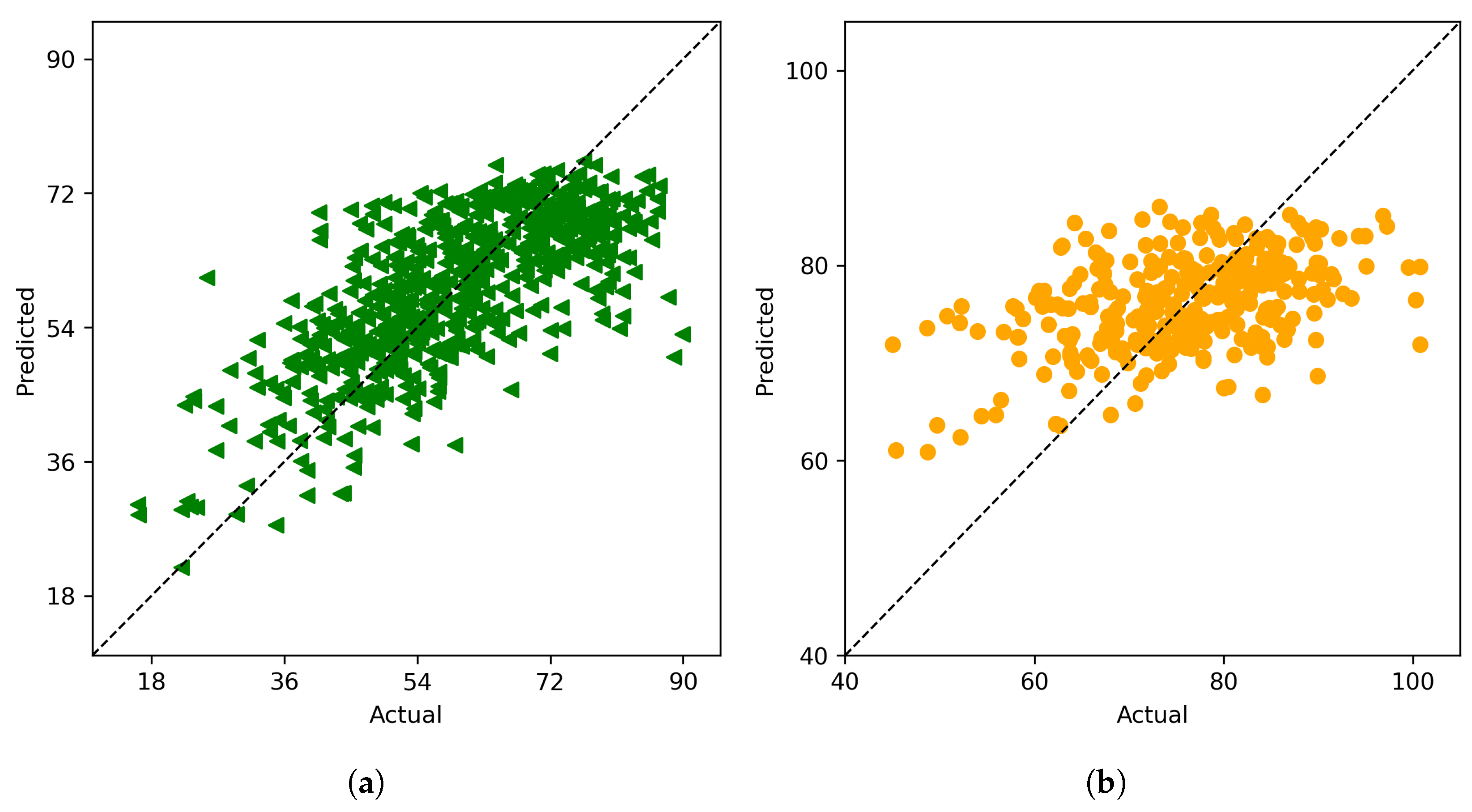
The results of cluster ensemble model points to an important fact that combining data from the different fields appropriately leads to much better accuracy of the individual tasks hence pointing to the fact that the different fields are indeed related in some way. The cluster ensemble model is able to identify such types of combinations efficiently and leverage the individual models through the ensemble weights which enables it to provide predictions with much higher accuracy compared to the field ensemble model. The potential for this type of learning task in a large breeding program could help to overcome problems with class imbalance that can be common in breeding programs due to skewed representation of genetic backgrounds. Genomic and pheomic prediction can be biased with improved prediction performance for large classes, but can fail on smaller subsets of data. Data driven ensemble approaches can help to increase overall accuracy and confidence in predictions made across breeding programs and be more precise in all genetic backgrounds.
Even though the cluster ensemble approach is a significant improvement over the field ensemble approach it is not significantly better than a simple random forest on the whole data. This we believe happens because the dataset used here is not sufficiently large to produce a significant increase in accuracy for the cluster ensemble model. Larger breeding programs resulting in extensive datasets can generate multiple clusters with ample data, enhancing the accuracy of individual tasks and ultimately boosting the accuracy of the ensemble model.
4.2. Analysis Using Soil Data
Our analysis of soil data for end season yield prediction followed the same principle as that of hyperspectral reflectance data. To obtain the best model we fitted several models using a eighty-twenty train-test split and 3-fold cross validation results of which are shown in Table 10. It is clearly evident that random forest provides the best accuracy compared to other models. The actual vs predicted plot for soil data using random forest is given in Figure 4b. An interesting observation is that, across all the different models, soil data outperforms hyperspectral data in predicting end season yield, suggesting that soil data alone may not fully account for the genetic characteristics of the plant, which spectral data takes into consideration. Considering that these field tests involve genotype comparisons, it can be concluded that adjustments can be made using spectral data to improve yield comparisons derived from soil data.
To identify the optimal subset of features for predicting end-season yield using soil data, we employed a backward feature selection approach similar to that used for hyperspectral data. The results of our feature selection analysis are summarized in Table 11. Our analysis indicates that a subset of just three features (MM_K, MM_MG, and MM_PH) is sufficient for predicting end-season yield with an accuracy comparable to that achieved using the full dataset.
In order to investigate if combining the two modalities can help predict yield with higher accuracy we combined the ten vegetation indices with three soil indicators and fitted a random forest model using eighty-twenty train test split and 3-fold cross validation. The resulting accuracy of this model was 0.76, which did not represent a significant increase compared to the accuracy achieved using only soil data. However, it is possible that more sophisticated multimodal learning algorithms, utilizing larger datasets, could more effectively combine these two modalities to yield predictions with higher accuracy. Further investigation is needed to fully explore the potential of combining these data modalities for yield prediction.
we analyzed is one that uses features from both the soil data and the vegetation indices.
We created a Random Forest model using the vegetation indices(table 8) and soil data (section 2.2) as features. The model tried to predict the yield column based on these features, and was trained on a dataset of around 3000 entries. To prevent significant imbalances between the number of features that were vegetation indices and the number of features that were soil data, we used the same number of feature columns for both types of features. Thus, the effects of the features on the results of the model would not be inherently skewed because of initial skewness in the cardinality of input feature type. We split our yield data into a 80-20 training-testing split and then fit the training data to the model.
The high accuracy of the models was achieved through hyperparameter optimization. We experiment with different optimizers and hyperparameter values for the max depth, the max-features type, the minimum samples in a leaf, the minimum samples per leaf, and the number of estimators. We choose the setting that optimizes for the highest accuracy. We test:
Table 7.
Hyperparameters
| Hyperparameter | Values |
|---|---|
| bootstrap | True, False |
| max_depth | 10, 20, 30, 40, 50, 60, 70, 80, 90, 100, None |
| max_features | auto, sqrt |
| min_samples_leaf | 1, 2, 4 |
| min_samples_split | 2, 5, 10 |
| n_estimators | 200, 400, 600, 800, 1000, 1200, 1400, 1600, 1800, 2000 |
The hyperparameter search yields optimal accuracy at the following hyperparameter values:
Table 8.
Hyperparameters
| Hyperparameter | Value |
|---|---|
| n_estimators | 400 |
| min_samples_split | 2 |
| min_samples_leaf | 1 |
| max_features | sqrt |
| max_depth | None |
| bootstrap | False |
Our results showed that there was no significant difference in the accuracy of our machine learning model when using multiple reflectance type data(i.e Band A, Band B, Band C), compared to using only one band of reflectance data for features. The Random Forest model that used multiple different bands achieved an accuracy of 0.77, while the Random Forest model that only used one reflectance band achieved an accuracy of 0.75. Thus, it can be concluded that collecting data from multiple reflectance bands may not be necessary for significant improvement in the accuracy of harvest yield
4.3. Feature Importance
Using the Random Forest model created, we determined the most important features of our model consisting of both vegetation indices and reflectance data. The most important features can be found in figure X.
Table 9.
Table Title
| Variable | Value |
|---|---|
| Population | 0.318527 |
| DDI_1 | 0.088559 |
| Clre_1 | 0.070222 |
| MM_P1 | 0.068096 |
| Clre_3 | 0.036757 |
| MM_CLAY | 0.035482 |
| MM_PH | 0.033846 |
| DPI_1 | 0.033274 |
| GNDV_3 | 0.031830 |
| Clre_2 | 0.029058 |
| MM_SILT | 0.027715 |
| MM_K | 0.023197 |
| MM_MG | 0.020231 |
| GNDV_1 | 0.017468 |
| MM_SAND | 0.016942 |
| Cl_1 | 0.015149 |
| Cl_3 | 0.014004 |
| DDI_2 | 0.013723 |
| DDI_3 | 0.013481 |
| MM_OM | 0.013148 |
Table 10.
Test accuracy (measured by ) for fitted models using soil data.
| Model | Accuracy |
| Linear Regression | 0.69 |
| Ridge Regression | 0.68 |
| LASSO | 0.68 |
| Random Forest | 0.73 |
Table 11.
Test accuracies of (measured by ) backward feature selection using random forest for soil data.
Table 11.
Test accuracies of (measured by ) backward feature selection using random forest for soil data.
| Number of features | Accuracy |
| 5 | 0.74 |
| 3 | 0.70 |
| 2 | 0.68 |
5. Conclusions
In this study we explored the task of soybean end season yield prediction using two modalities, the hyperspectral reflectance and soil data. We used fifty two vegetation indices computed from the raw hyperspectral bands (Table A1) for our analysis and obtained better results compared to raw wavelengths. This aligns with previous work that has shown significant improvements by using known indices over raw reflectance dataLi et al. [2], Parmley et al. [11]. Our study indicated that data on only twelve wavelengths are necessary compared to six hundred wavelengths.We also demonstrated the effectiveness of ensemble methods, particularly the cluster ensemble methods for soybean yield prediction, using ten vegetation indices. We find that the cluster ensemble model performs significantly better compared to the field ensemble model even though we do not see any significant improvement over a simple random forest approach over the full dataset. This happens most probably due to the size and nature of the data used for this study but larger datasets can potentially give rise to better accuracy compared to a simple model. Soil data shows a much higher potential for predicting yield compared to hyperspectral both with original data of ten features and subset of three features but combining soil data with hyperspectral doesn’t lead to any significant increase in accuracy. Such results may not hold for more dissimilar genotypes due to the genetic differences that may be learned from the spectral data.
There are two important aspects of this study. First obtaining smaller subsets for both modalities which can predict yield with same accuracy as that of full set of features signifies that the process of data collection can be efficiently streamlined cutting both cost and labour. Secondly our cluster ensemble model indicates that in case of very large breeding programs data driven methods for obtaining subgroups will always result in better ensemble models compared to manual grouping. Future research in this field will involve investigating the potential benefits of blocking the data based on the layout of the breeding program, grouping lines with similar genetic backgrounds, to determine whether it can lead to more accurate models. Additionally, the development of multimodal learning models will be explored with the aim of improving prediction accuracy by leveraging multiple data modalities.
Author Contributions
Souradeep Chattopadhyay processed soil and hyperspectral reflectance data, designed and coded the algorithms, generated results, and prepared the first draft. Aditya Gupta processed soil and vegetation data, applied machine learning algorithms to run the analysis, generated results, and prepared the first draft. Matthew Carroll performed field experiments, provided agronomic interpretation of yield data and results, and edited the manuscript. Joscif Raigne provided agronomic interpretation of yield data and results and edited the manuscript. Baskar Ganapathysubramanian participated in the project’s development and reviewed the manuscript. Asheesh K. Singh conceptualized the experiments, supervised the research, and edited the manuscript. Soumik Sarkar conceptualized the experiments, supervised the research, and edited the manuscript.
Acknowledgments
The authors thank staff and student members of SinghSoybean group at Iowa State University, particularly Brian Scott, Will Doepke, Jennifer Hicks, Ryan Dunn, and Sam Blair for their assistance with field experiments and phenotyping. The authors sincerely appreciate the funding support from the Iowa Soybean Association (A.K.S.), North Central Soybean Research Program (A.K.S.), USDA CRIS project IOW04714 (A.K.S.), AI Institute for Resilient Agriculture (USDA-NIFA #2021-647021-35329) (B.G., S.S., A.K.S.), COALESCE: COntext Aware LEarning for Sustainable CybEr-Agricultural Systems (CPS Frontier #1954556) (S.S., A.K.S., B.G.), Smart Integrated Farm Network for Rural Agricultural Communities (SIRAC) (NSF S & CC #1952045) (A.K.S., S.S.), RF Baker Center for Plant Breeding (A.K.S.), and Plant Sciences Institute (A.K.S., S.S., B.G.). M.E.C. was partially supported by a graduate assistantship through NSF NRT Predictive Plant Phenomics project.
Appendix A Table of Vegetation Indices
Table A1.
Summary of the 52 vegetation indices. Here Tx denote the hyperspectral reflectance value at x nm.
Table A1.
Summary of the 52 vegetation indices. Here Tx denote the hyperspectral reflectance value at x nm.
| Full form | Spectral Index/Ratio | Formula |
|---|---|---|
| Curvature index | Cl | |
| Chlorophyll Index red-edge | Clre | |
| Datt1 | ||
| Datt4 | ||
| Datt6 | ||
| Double difference index | DDI | |
| Double peak index | DPI | |
| Gitelson2 | ||
| Green normalized difference vegetation index | GNDVI | |
| Modified chlorphyll absorption ratio index | MCARI | |
| MCARI3 | ||
| Modified normalized difference | MND1 | |
| MND2 | ||
| Modified simple ratio | mSR | |
| Modified simple ratio 2 | mSR2 | |
| MERIS terrestrail cholrophyll index | MTCI | |
| Modified traingular vegetation index 1 | MTVI1 | |
| Normalized difference 550/531 | ND1 | |
| Normalized difference 682/553 | ND2 | |
| Normalized difference chlorophyll | NDchl | |
| Normalized difference red edge | NDRE | |
| Normalized difference vegetation index | NDVI1 | |
| NDVI2 | ||
| NDVI3 | ||
| Normalized pigment cholrophyll index | NPCL | |
| Normalized difference pigment index | NPQI | |
| Optimized soil-adjusted vegetation index | OSAVI | |
| Plant biochemical index | PBI | |
| Plant pigment ratio | PPR | |
| Physiological reference index | PRI | |
| Pigment-specific normalized difference | PSNDb1 | |
| PSNDc1 | ||
| PSNDc2 | ||
| Plant senescence reflectance index | PSRI | |
| Pigment-specific simple ratio | PSSRc1 | |
| PSSRc2 | ||
| Photosynthetic vigor ratio | PVR | |
| Plant water index | PWI | |
| Renormalized difference vegetation index | RDVI | |
| Red-edge stress vegatation index | RVSI | |
| Soil-adjusted vegatation index | SAVI | |
| Structure intensive pigment index | SIPI | |
| Simple ratio | SR1 | |
| SR2 | ||
| SR3 | ||
| SR4 | ||
| Disease -water stress index 4 | DSWI-4 | |
| Simple ratio pigment index | SRPI | |
| Transformed chlorophyll absorption ratio | TCARI | |
| Traingular cholrophyll index | TCI | |
| Triangular vegetation index | TVI | |
| Water band index | WBI |
References
- Singh, D.P.; Singh, A.K.; Singh, A. Plant breeding and cultivar development; Academic Press, 2021.
- Li, Z.; Chen, Z.; Cheng, Q.; Duan, F.; Sui, R.; Huang, X.; Xu, H. UAV-Based Hyperspectral and Ensemble Machine Learning for Predicting Yield in Winter Wheat. Agronomy 2022, 12. [Google Scholar] [CrossRef]
- Yoosefzadeh-Najafabadi, M.; Torabi, S.; Tulpan, D.; Rajcan, I.; Eskandari, M. Genome-wide association studies of soybean yield-related hyperspectral reflectance bands using machine learning-mediated data integration methods. Frontiers in plant science 2021, p. 2555. [CrossRef]
- Chiozza, M.V.; Parmley, K.A.; Higgins, R.H.; Singh, A.K.; Miguez, F.E. Comparative prediction accuracy of hyperspectral bands for different soybean crop variables: From leaf area to seed composition. Field Crops Research 2021, 271, 108260. [Google Scholar] [CrossRef]
- Shook, J.; Gangopadhyay, T.; Wu, L.; Ganapathysubramanian, B.; Sarkar, S.; Singh, A.K. Crop yield prediction integrating genotype and weather variables using deep learning. PLOS ONE 2021, 16, 1–19. [Google Scholar] [CrossRef] [PubMed]
- Riera, L.G.; Carroll, M.E.; Zhang, Z.; Shook, J.M.; Ghosal, S.; Gao, T.; Singh, A.; Bhattacharya, S.; Ganapathysubramanian, B.; Singh, A.K.; Sarkar, S. Deep Multiview Image Fusion for Soybean Yield Estimation in Breeding Applications. Plant Phenomics 2021, 2021, 9846470. [Google Scholar] [CrossRef] [PubMed]
- Guo, W.; Carroll, M.E.; Singh, A.; Swetnam, T.L.; Merchant, N.; Sarkar, S.; Singh, A.K.; Ganapathysubramanian, B. UAS-Based Plant Phenotyping for Research and Breeding Applications. Plant Phenomics 2021, 2021, 9840192. [Google Scholar] [CrossRef] [PubMed]
- Singh, A.K.; Singh, A.; Sarkar, S.; Ganapathysubramanian, B.; Schapaugh, W.; Miguez, F.E.; Carley, C.N.; Carroll, M.E.; Chiozza, M.V.; Chiteri, K.O.; Falk, K.G.; Jones, S.E.; Jubery, T.Z.; Mirnezami, S.V.; Nagasubramanian, K.; Parmley, K.A.; Rairdin, A.M.; Shook, J.M.; Van der Laan, L.; Young, T.J.; Zhang, J., High-Throughput Phenotyping in Soybean. In High-Throughput Crop Phenotyping; Zhou, J.; Nguyen, H.T., Eds.; Springer International Publishing: Cham, 2021; pp. 129–163 [CrossRef]
- Nagasubramanian, K.; Jones, S.; Sarkar, S.; Singh, A.K.; Singh, A.; Ganapathysubramanian, B. Hyperspectral band selection using genetic algorithm and support vector machines for early identification of charcoal rot disease in soybean stems. Plant methods 2018, 14, 86. [Google Scholar] [CrossRef] [PubMed]
- Parmley, K.A.; Higgins, R.H.; Ganapathysubramanian, B.; Sarkar, S.; Singh, A.K. Machine Learning Approach for Prescriptive Plant Breeding. Scientific Reports 2019, 9, 17132. [Google Scholar] [CrossRef] [PubMed]
- Parmley, K.; Nagasubramanian, K.; Sarkar, S.; Ganapathysubramanian, B.; Singh, A.K. Development of Optimized Phenomic Predictors for Efficient Plant Breeding Decisions Using Phenomic-Assisted Selection in Soybean. Plant Phenomics 2019, 2019, 5809404. [Google Scholar] [CrossRef] [PubMed]
- Gupta, A.; Sharma, B.; Chingtham, P. Forecast of Earthquake Magnitude for North-West (NW) Indian Region Using Machine Learning Techniques 2023. [CrossRef]
- Sarkar, S.; Ganapathysubramanian, B.; Singh, A.; Fotouhi, F.; Kar, S.; Nagasubramanian, K.; Chowdhary, G.; Das, S.K.; Kantor, G.; Krishnamurthy, A.; et al. . Cyber-agricultural systems for crop breeding and sustainable production. Trends in Plant Science 2023. [Google Scholar] [CrossRef] [PubMed]
- Singh, A.K.; Singh, A.; Sarkar, S.; Ganapathysubramanian, B.; Schapaugh, W.; Miguez, F.E.; Carley, C.N.; Carroll, M.E.; Chiozza, M.V.; Chiteri, K.O. High-throughput phenotyping in soybean. High-throughput crop phenotyping 2021, pp. 129–163. [CrossRef]
- Herr, A.W.; Adak, A.; Carroll, M.E.; Elango, D.; Kar, S.; Li, C.; Jones, S.E.; Carter, A.H.; Murray, S.C.; Paterson, A.; others. Unoccupied aerial systems imagery for phenotyping in cotton, maize, soybean, and wheat breeding. Crop Science 2023, 63, 1722–1749. [Google Scholar] [CrossRef]
- Young, T.J.; Jubery, T.Z.; Carley, C.N.; Carroll, M.; Sarkar, S.; Singh, A.K.; Singh, A.; Ganapathysubramanian, B. “Canopy fingerprints” for characterizing three-dimensional point cloud data of soybean canopies. Frontiers in Plant Science 2023, 14, 1141153. [Google Scholar] [CrossRef] [PubMed]
- Gupta, A.; Tayal, V.K. Analysis of Twitter Sentiment to Predict Financial Trends. 2023 International Conference on Artificial Intelligence and Smart Communication (AISC). IEEE, 2023, pp. 1027–1031. [CrossRef]
- Huang, F.; Xie, G.; Xiao, R. Research on Ensemble Learning. 2009 International Conference on Artificial Intelligence and Computational Intelligence, 2009, Vol. 3, pp. 249–252. [CrossRef]
- Khaledian, Y.; Miller, B.A. Selecting appropriate machine learning methods for digital soil mapping. Applied Mathematical Modelling 2020, 81, 401–418. [Google Scholar] [CrossRef]
- Bai, G.; Ge, Y.; Hussain, W.; Baenziger, P.S.; Graef, G. A multi-sensor system for high throughput field phenotyping in soybean and wheat breeding. Computers and Electronics in Agriculture 2016, 128, 181–192. [Google Scholar] [CrossRef]
- Raschka, S. MLxtend: Providing machine learning and data science utilities and extensions to Python’s scientific computing stack. The Journal of Open Source Software 2018, 3. [Google Scholar] [CrossRef]
- Breiman, L. Random Forests. Machine Learning 2001, 45, 5–32. [Google Scholar] [CrossRef]
- Abdillah, A.; Sutisna, A.; Tarjiah, I.; Fitria, D.; Widiyarto, T. Application of Multinomial Logistic Regression to analyze learning difficulties in statistics courses. Journal of Physics: Conference Series 2020, 1490, 012012. [Google Scholar] [CrossRef]
- MacQueen, J. Some methods for classification and analysis of multivariate observations. Proceedings of the Fifth Berkeley Symposium on Mathematical Statistics and Probability, Volume 1: Statistics; University of California Press: Berkeley, California, 1967; pp. 281–297. [Google Scholar]
- Pedregosa, F.; Varoquaux, G.; Gramfort, A.; Michel, V.; Thirion, B.; Grisel, O.; Blondel, M.; Prettenhofer, P.; Weiss, R.; Dubourg, V.; Vanderplas, J.; Passos, A.; Cournapeau, D.; Brucher, M.; Perrot, M.; Duchesnay, E. Scikit-learn: Machine Learning in Python. Journal of Machine Learning Research 2011, 12, 2825–2830. [Google Scholar]
Figure 1.
Reflectance plot for wavelength’s 400 nm to 1000 nm for one plot. The red, green and blue bands represent wavelengths of the visible spectrum.
Figure 1.
Reflectance plot for wavelength’s 400 nm to 1000 nm for one plot. The red, green and blue bands represent wavelengths of the visible spectrum.
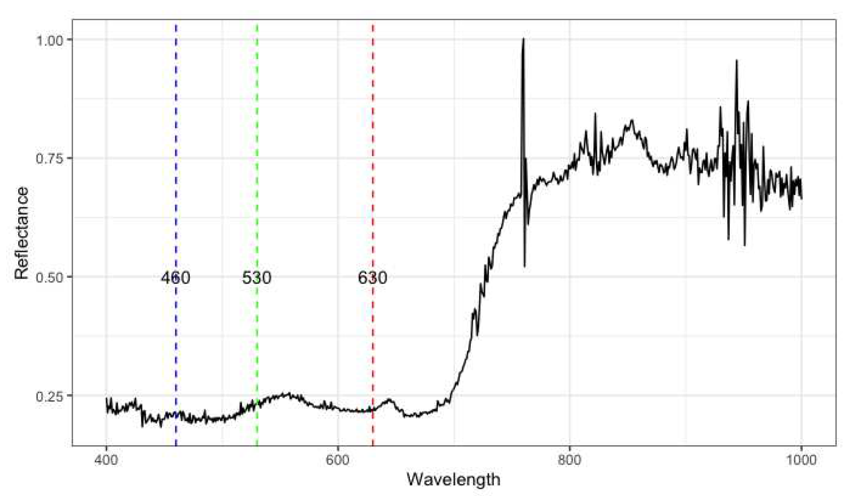
Figure 2.
From left to right: (a) The field ensemble model, (b) The cluster ensemble model.
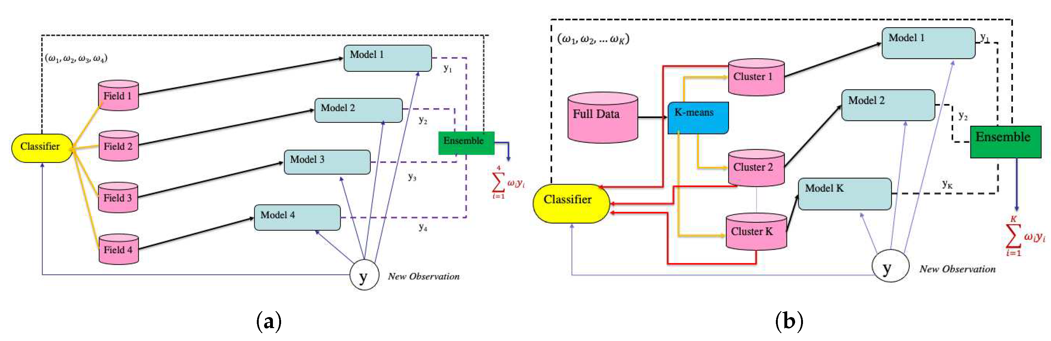
Table 1.
Number of datapoints in each of the four fields.
| Field No. | Number of observations |
| 1 | 770 |
| 2 | 912 |
| 3 | 800 |
| 4 | 679 |
Table 2.
Test accuracy (measured by ) for fitted models using vegetation indices.
| Model | Accuracy |
| Linear Regression | 0.46 |
| Ridge Regression | 0.45 |
| LASSO | 0.41 |
| Random Forest | 0.55 |
Table 3.
Test accuracy (measured by ) backward feature selection using random forest for different number of features.
Table 3.
Test accuracy (measured by ) backward feature selection using random forest for different number of features.
| Number of features | Accuracy |
| 40 | 0.55 |
| 20 | 0.53 |
| 10 | 0.50 |
| 5 | 0.47 |
Table 4.
Test accuracy (measured by ) for fitted random forest model for each of the four fields and the field ensemble model.
Table 4.
Test accuracy (measured by ) for fitted random forest model for each of the four fields and the field ensemble model.
| Field No. | Accuracy |
| 1 | 0.09 |
| 2 | -0.17 |
| 3 | -0.19 |
| 4 | -0.005 |
| Field ensemble | 0.21 |
Table 6.
Test accuracy (measured by ) for fitted random forest model on the two clusters, the cluster ensemble model.
Table 6.
Test accuracy (measured by ) for fitted random forest model on the two clusters, the cluster ensemble model.
| Cluster No. | Accuracy |
| 1 | 0.39 |
| 2 | 0.28 |
| Cluster ensemble | 0.51 |
Disclaimer/Publisher’s Note: The statements, opinions and data contained in all publications are solely those of the individual author(s) and contributor(s) and not of MDPI and/or the editor(s). MDPI and/or the editor(s) disclaim responsibility for any injury to people or property resulting from any ideas, methods, instructions or products referred to in the content. |
© 2023 by the authors. Licensee MDPI, Basel, Switzerland. This article is an open access article distributed under the terms and conditions of the Creative Commons Attribution (CC BY) license (http://creativecommons.org/licenses/by/4.0/).
Copyright: This open access article is published under a Creative Commons CC BY 4.0 license, which permit the free download, distribution, and reuse, provided that the author and preprint are cited in any reuse.


