1. Introduction
Agriculture directly impacts people's lives and is essential to the development of the global economy. However, pests in crops often cause great losses. Therefore, it is necessary to prevent pest control to ensure a high agricultural yield[
1]. Because of developments in science and technology, pest detection methods are continually changing[
2]. Early detection relies on field diagnosis by agricultural experts, but proper diagnosis is difficult due to the complexity of pest conditions, lack of qualified staff and inconsistent experience at the grassroots level. Furthermore, incorrect pest identification by farmers has led to an escalation in pesticide usage. This in turn has bolstered pest resistance[
3] and exacerbated the harm inflicted upon the natural environment.
An effective integrated pest automated monitoring system relies on a high-quality algorithm. With the development of image processing technology and deep learning, more and more scholars use pest image data and deep learning to identify pests, which improves the effectiveness of agricultural pest detection and is also the first application example of intelligent diagnosis. Classification and detection of agricultural pests is a crucial research field to help farmers effectively manage crops and take timely measures to reduce the harm of pests. Object detection models, which come in one-stage and two-stage varieties, are frequently employed in pest classification detection. One-stage models like YOLO[
4,
5,
6] and SSD[
7] are renowned for their rapid detection capabilities. In contrast, two-stage models like Fast R-CNN[
2] and Faster R-CNN[
9] excel in achieving high accuracy, albeit at a slower processing speed compared to their one-stage counterparts. The transformer model is introduced in 2017[
10] and has a lot of potential applications in AI. Based on its effectiveness in natural language processing (NLP)[
11], recent research has extended Transformer to the field of computer vision (CV)[
12]. In 2021 Swin Transformer[
13] was proposed as a universal backbone for CV, which achieves the latest SOTA on multiple dense prediction benchmarks. The differences between language and vision make the transition from language to vision difficult, such as the vast range of visual entity scales. But the Swin Transformer can solve this problem well. In this paper, we use a Vision Transformer with a shift window to detect pests.
Currently, two dataset-related issues affect pest detection: (1) The scarcity of high-quality datasets. There are only over 600 photos in eight pest datasets, reflecting the lack of agricultural pest datasets[
14]. (2) The challenges of detecting pests at multiple scales. The size difference between large and micro pests is large, up to 30 times in some cases. For example, the relative size of the largest pest in the LMPD2020 dataset is 0.9%, while the relative size of the smallest pest is only 0.03%. When the size difference of the test object is large, it is difficult for the test results at multiple scales to achieve a high accuracy simultaneously, and the problem of missing detection often occurs. Moreover, the Transformer also requires a large dataset for training.
In agriculture, there are few high-quality pest datasets available, and some datasets come from the web with poor clarity and different sizes. To improve the accuracy of pest identification, enable models to learn more complex semantic information from training data, and complement the agricultural dataset. This paper proposes a new pest detection method with two key functions: data generation using diffusion models and pest detection using Swin Transformers. The diffusion model[
15] is first introduced in 2015. It acts as a sequence of denoising autoencoders, and its goal is to remove Gaussian noise by continually applying it to the training images. A new diffusion model[
16] represents the novel state-of-the-art in-depth image generation. In picture-generating tasks, it outperforms the original SOTA: GAN (Generative Adversarial Networks)[
17] and performs well in a variety of applications, including CV, NLP, waveform signal processing, time series modeling and adversarial learning. The Denoising Diffusion Probabilistic Model was proposed later in 2020[
18] applying to image generation. In 2021 Open AI’s paper: Diffusion Model Beat GANs on Image Synthesis[
19] makes machine-generated data even more realistic than GAN. DALL-E2[
20] allows us to use text descriptions to generate the image we want.
Overall, this paper mainly makes the following contributions:
(1) RS Transformer, a novel model based on the Region Proposal Network (RPN), Swin Transformer, and ROI Align, for few-shot detection of pests at different scales.
(2) RGSDD, a new training strategy method Randomly Generate Stable Diffusion Dataset is introduced to expand small pest images to effectively classify and detect pests in a short period
(3) Comprehensive experiments on the pest dataset confirmed the success of our proposed methods contrasting with SSD[
7], Faster R-CNN[
9], YOLOv3[
4], YOLOv4[
5], YOLOv5m[
6], YOLOv8 and DETR[
21].
2. Materials and Methods
2.1. Pest Dataset
2.1.1. Real Pest Image Dataset
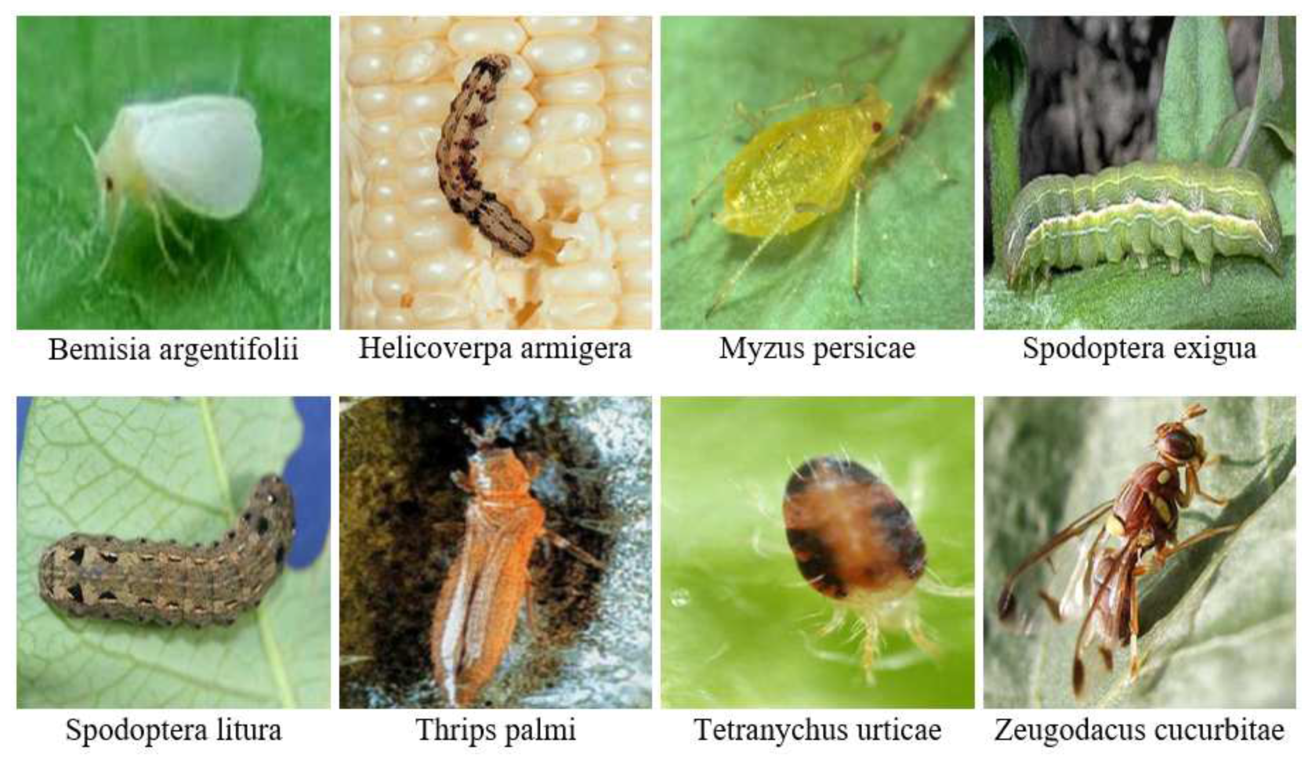
This study focuses on crops of high economic value. As a result, the selection of agricultural pests is based on small sample sizes. First, we went to the Beizang Village experimental field next to the Daxing Campus of Beijing University of Civil Engineering and Architecture to take photos with an iPhone 12 pro-Max and collected 400 pictures of pests. Secondly, pests were searched for on the IPMImages database[
22], National Bureau of Agricultural Insect Resources (NBAIR), Google, Bing, etc. Eight common pests are used as the foundation: (1)Tetranychus urticae, TU (2)Bemisia argentifolii, BA (3)Zeugodacus cucurbitae, ZC (4)Thrips palmi, TP (5)Myzus persicae, MP (6)Spodoptera litura, SL (7)Spodoptera exigua, SE (8)Helicoverpa armigera HA. Figure.1 displays a few representative photos from the dataset. Eventually, the resulting pest dataset grows to 1009.
Figure 1.
The pests dataset.
Figure 1.
The pests dataset.
2.1.2. Dataset Generation
Stable diffusion was released by Open AI in 2022[
23], a model that can be used to generate detailed images conditioned on text descriptions.
The diffusion model, which produces samples that fit the data after a finite amount of time, is a parameterized Markov chain trained via variational inference. [
18]. As seen in
Figure 2, the
and the
can be separated from the entire diffusion model. It is commonly understood that the forward diffusion process is constantly adding Gaussian noise to the image, making it "unrecognizable", while the reverse process reduces the noise and then restores the image. The core formula of the diffusion model is,
where
is experiment constant and it will decrease as t increases.
is a standard Gaussian noise distribution
The overall structure of the diffusion model is shown in
Figure 3. It contains three models. The first is the CLIP model (Contrastive Language-Image Pre-Training), which is a text encoder that converts text into vectors as input. The image is then generated using the Diffusion model. It is performed in the potential space of the compressed image, so the input and output of the expanded model are the image features of the potential space, not the pixels of the image itself. During the training of the latent diffusion model, an encoder is used to obtain the potentials of the picture training set, which are used in the forward diffusion process (each step adds more noise to the latent representation). At inference generation, the decoder part of VAE (Variational Auto-Encoder) converts the denoised latent signal generated by the reverse diffusion process back into an image format.
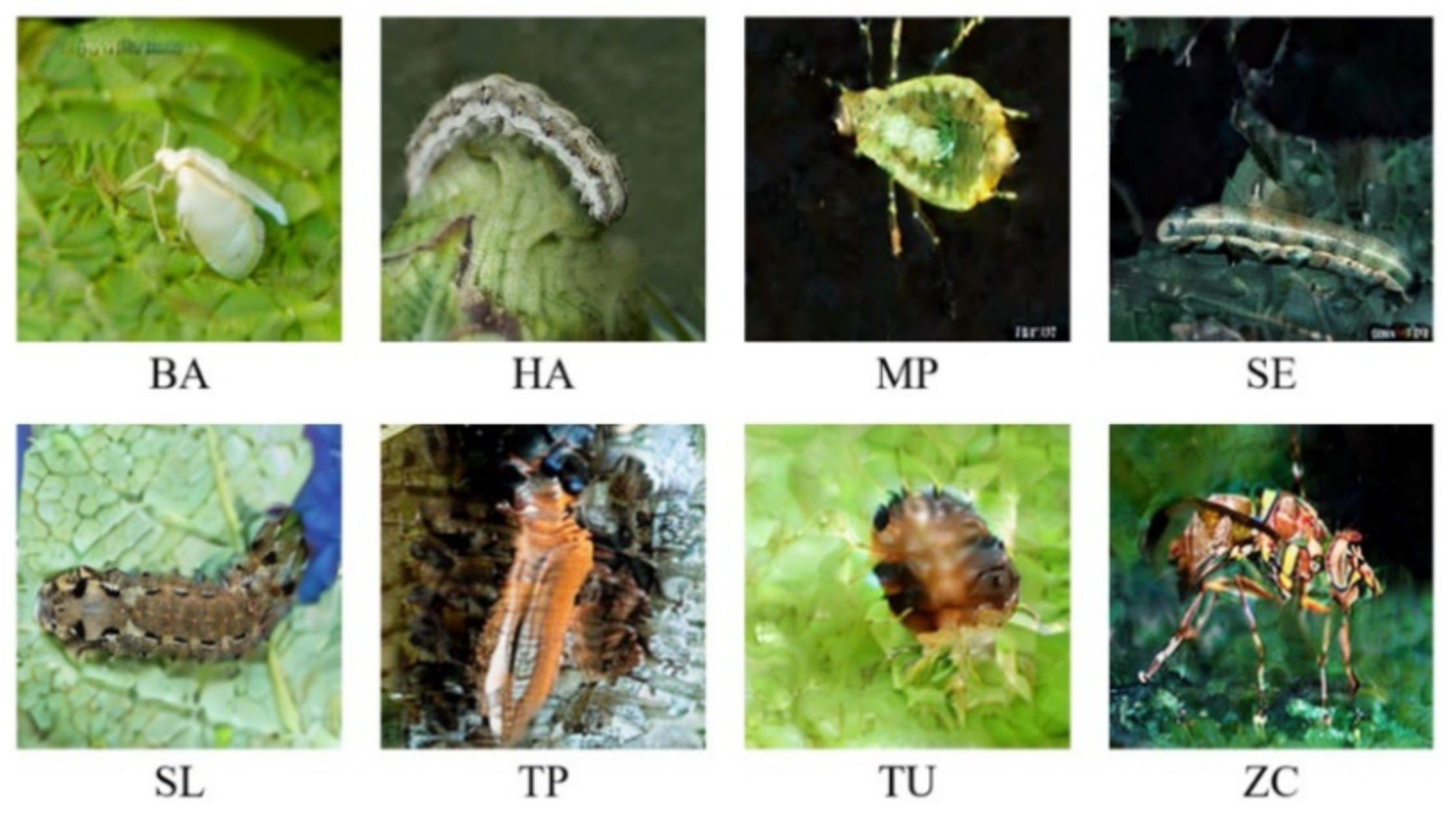
A stable diffusion model is trained using a real pest dataset. The images generated by Stable Diffusion are 299×299 as shown in
Figure 4. To increase the chance of generating pest images, we chose captions that contain any word from the following list of words: [BA, HA, MP, SE, SL, TP, TU, ZC]. After carefully eliminating the last few false positives, we gathered 512 produced pests.
2.1.3. Dataset Enhancement
In this study, the original image was processed using enhancement methods such as rotation, translation, flipping, and noise addition., and the enhancement technique AutoAugmentation[
24] is applied to operate the color of images. Finally, we got 36,122 pest images.
2.2. Framework of the Proposed Method
In this paper, R-CNN[
25] is replaced by Swin Transformer and applied to pest target detection tasks. A new object detection method, RS Transformer, is proposed. The advantages of our scheme are:
First, a new feature extraction method for the Swin Transformer is proposed and used in the feature extraction module. It improves the alignment of global features. The localization accuracy is improved and the computing cost of the transformer is significantly reduced by the shift window model.
Second, RS Transformer is proposed which adds RPN, ROI Align, and Feature map.
Third, a new data composition method RGSDD is proposed. This method is used to train the stable diffusion model of the real images collected before, and 512 images are generated randomly mixed with 10%, 20%, 30%,40%, and 50% of the number of real images.
2.3. RS Transformer
RS Transformer is a two-stage model (
Figure 5). It first extracts features using Swin Transformer and then generates a series of region proposals.
2.3.1. Swin Transformer Backbone
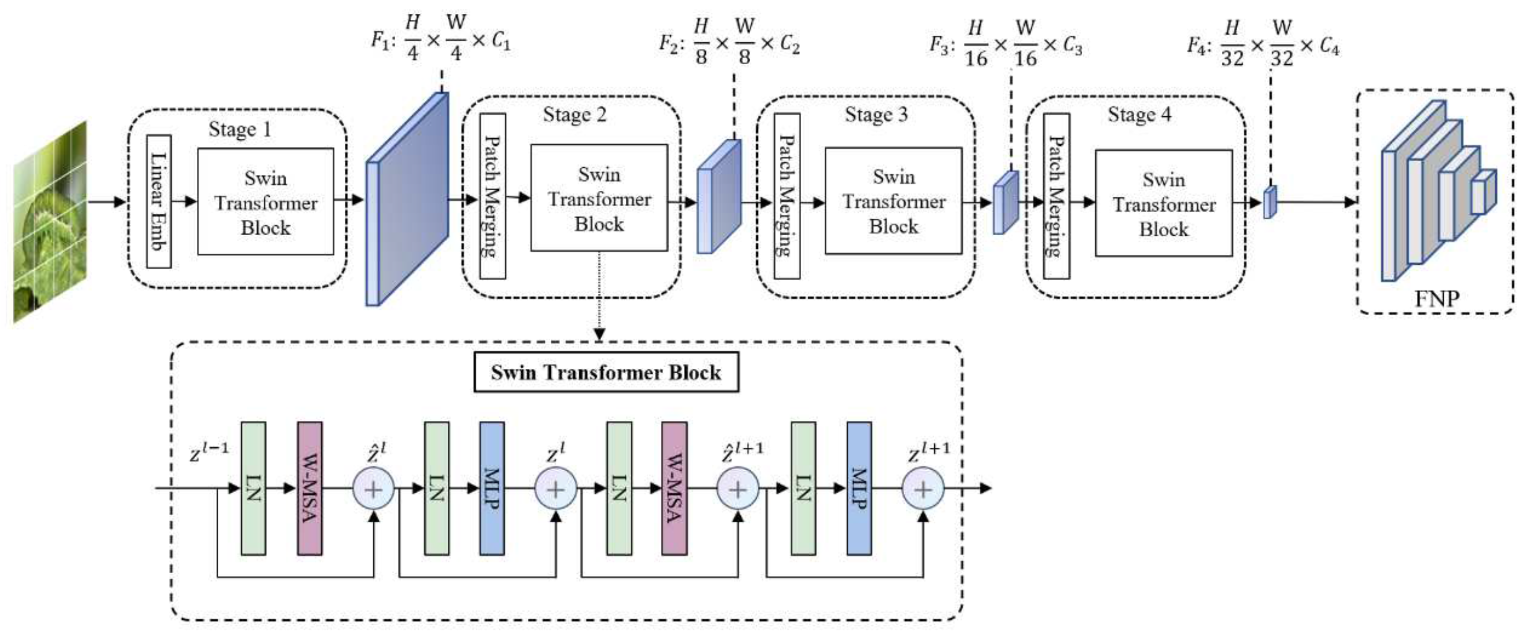
The Swin Transformer backbone is introduced in
Figure 6. Compared to traditional CNN models, it has stronger feature extraction capabilities, incorporates CNN's local and hierarchical structure, and utilizes attention mechanisms to produce a more interpretable model and examine the attention distribution.
A 2-layer MLP (Multi-layer Perceptron) with GELU non-linearity follows a shifted window-based MSA module (W-MSA) in the Swin Transformer block. Each MSA module (Multi-head Self-Attention) and each MLP have an LN (Layer Norm) layer applied before them, and each module also has a residual connection applied after it. Supposing each window contains
patches, the computational complexity of a global MSA module and image-based window
patches are:
The shift window partitioning method can be used to compute the backbones of two consecutive Swin Transformers and is denoted as follows:
where
and
represent the output of W-MSA and MLP of the
block, respectively.
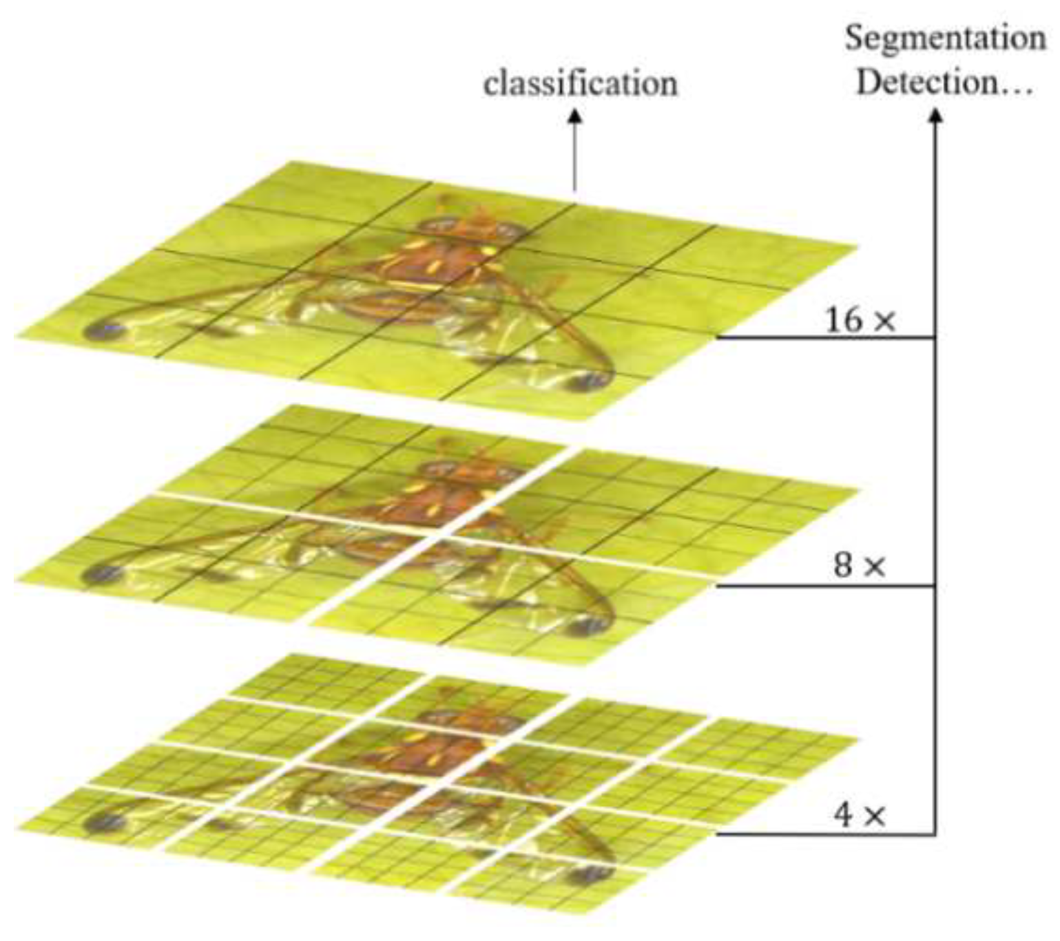
Swin Transformer constructs hierarchical feature graphs and adopts a complexity calculation method with linear image size. A sample diagram of a hierarchy of small patch size is shown in
Figure 7. In the deeper Transformer layers, it begins with small-size patches and eventually integrates nearby patches. By using patch splitting modules like ViT, RGB images are divided into non-overlapping patches, and employ a patch size of
, making each patch's feature dimension
. This fundamental feature is projected to any dimension (designated
) using a linear embedding layer.
2.3.2. RS Transformer neck: FPN
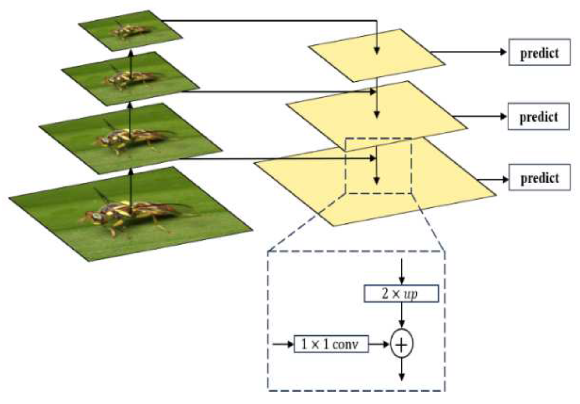
FPN (Feature Pyramid Networks) is proposed to achieve a better fusion of feature maps. As illustrated in
Figure 8, the purpose of FPN is to integrate feature maps from the bottom layer to the top layer to fully utilize the extracted features at each stage.
FPN produces a feature pyramid, not just a feature map. Pyramid after RPN will produce many region proposals. These region proposals are produced by RPN, and ROI is cut out according to the region proposal for subsequent classification and regression prediction. We use a formula to determine which k the ROI of wide w and high h should be cut from:
Here 224 represents the size of the ImageNet image used for pre-training. represents the level at which the ROI of the area is should be. Large-scale ROI should be cut from the feature map of low resolution, which is conducive to the detection of large targets, and small-scale ROI should be cut from the feature map of high resolution, which is conducive to the detection of small targets.
2.3.3. RS Transformer Head: RPN, ROI Align
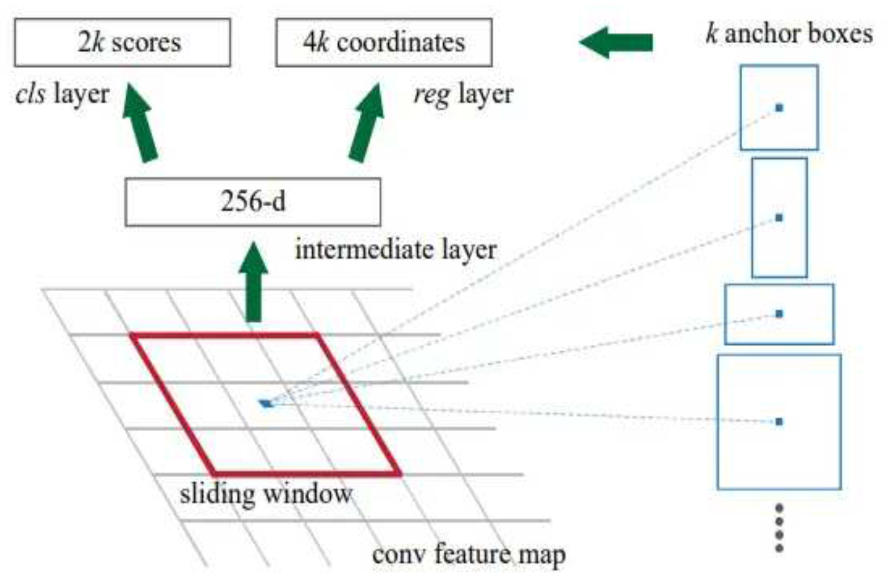
To achieve the prediction of coordinates and scores of each regional suggestion box while extracting features, the RPN network adds a regression layer (reg-layer) and a classification layer (cls-layer) to the Swin Transformer.
Figure 9 depicts the RPN working principle. RPN centers on a pixel of the last layer feature map and traverses the feature map through a 3×3 sliding window. The pixel points mapped from the center of the sliding window to the original image are anchor points. Taking the anchor point as the original image center, using 15 preset anchor boxes with 5 different areas (32×32, 64×64, 128×128, 256×256, 512×512), and three distinct aspect ratios (2:1, 1:1, and 1:2), the original candidate region, k=15 was obtained. RPN sends the candidate regions in the k anchor boxes to the regression layer and the category layer respectively for boundary regression and classification prediction. The regression layer predicts the frame coordinates (X, Y, W, H), so the output is 4k; the classification layer predicts the type, target, and background, so the output is 2k. Each anchor is then evaluated with initial over-boundary screening and Non-Maximum Suppression (NMS) from largest to smallest to retain the top 1000 or 2000 scores. Finally, the candidate boundaries of prediction as background in the classification layer are removed, and the candidate boundaries of prediction as a target are retained.
ROI Align
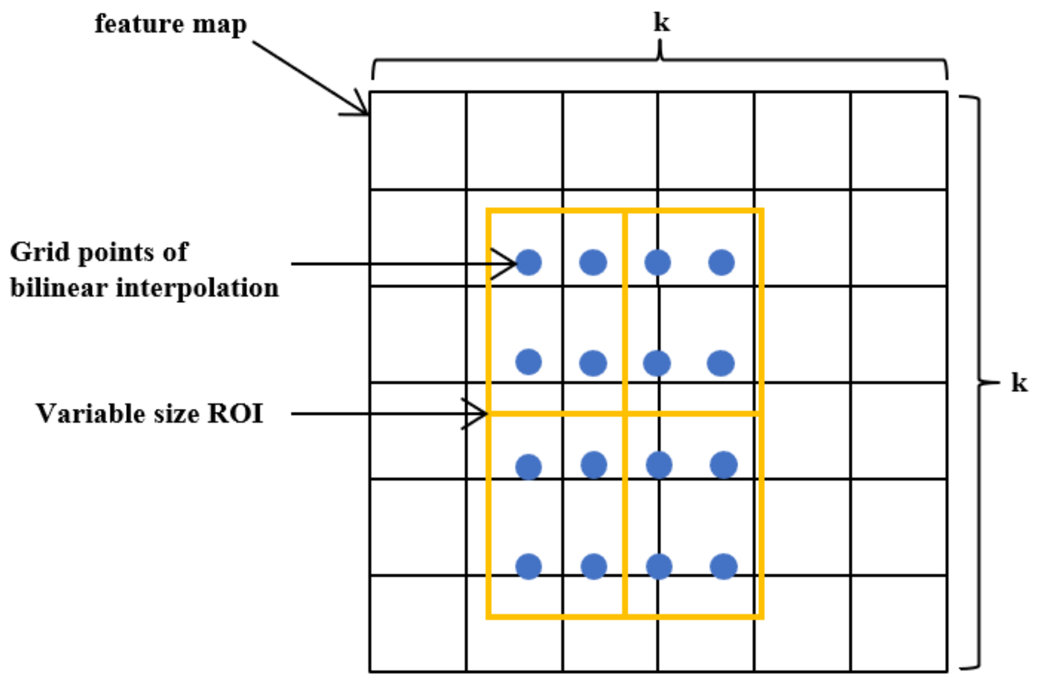
The function of ROI Pool and ROI Align is to find the feature map corresponding to the candidate box, then process the feature map of different size proportions into a fixed size, so that it can be input into the subsequent fixed-size network. Mask RCNN proposed an ROI Alignment[
26] based on the ROI pool. The bilinear interpolation method is used to determine the eigenvalue of each pixel in the region of interest of the original image, which avoids the error caused by quantization operation and improves the accuracy of frame prediction and mask prediction.
ROI Alignment algorithm's primary steps are: (1) Traverse each candidate region on the feature map, keeping the floating-point boundary unquantized; (2) In
Figure 10, the candidate region is evenly divided into k×k bins, and the edge of each bin keeps the floating-point number without quantization; (3) Take 2×2 sample points for each bin, and use the bilinear interpolation method to calculate the pixel values of each sampling point's neighboring four pixels. Finally, the pixel value in each bin is maximized to obtain the value of each bin.
3. Results and Discussion
This section may be divided by subheadings. It should provide a concise and precise description of the experimental results, their interpretation, as well as the experimental conclusions that can be drawn.
3.1. Experiment Setup
The experiments are conducted on the Autodl platform, which provides low-cost GPU computing power and a configuration environment that can be rented at any time. For researchers and universities without high-performance GPUs or servers, Autodl offers a wide range of high-performance GPUs to use. The experiments were implemented using the Pytorch 1.10.0 framework, Python 3.8, CUDA 11.3, and Nvidia RTX 2080Ti GPUs with 11GB memory.
3.2. Evaluation Indicator
To evaluate the performance of the proposed model, Precision, Average Precision (AP), Recall, Precision-Recall Curve, mean Average Precision (mAP), and F1 Score were selected as evaluation metrics.
Average Precision (AP): The average precision under different recall rates. The higher the accuracy, the higher the AP.
(11)
Recall: The average recall rate at different levels of precision. The higher the recall, the higher the AR.
mean Average Precision (mAP): During the picture categorization procedure, it is usually a multi-classification problem. According to the above calculation process, the AP of each analog is obtained, and then the average value is mAP.
(13)
3.3. Experimental Baselines
To evaluate the performance of RS Transformer, SSD[
7], Faster R-CNN[
9], YOLOv3[
4], YOLOv4[
5] and YOLOv5m[
6], YOLOv8 and DETR[
27] were chosen as baseline models for comparison.
Table 1.
Different baselines.
Table 1.
Different baselines.
| Models |
Backbone |
Parameters(M) |
| SSD |
VGG16 |
28.32 |
| Faster R-CNN |
VGG16 |
138 |
| YOLOv3 |
Darknet-53 |
64.46 |
| YOLOv4 |
CSPDarknet53 |
5.55 |
| YOLOv5m |
CSPDarknet53 |
20.66 |
| YOLOv8 |
C2f |
30.13 |
| DETR |
ResNet-50 |
40.34 |
| RS Transformer |
Swin Transformer |
30.17 |
3.4. Experimental Results and Analysis
On a dataset with five models, we assessed the performance of popular deep learning models to adequately illustrate the performance of the proposed model (
Table 2). Enter a fixed image resolution with a size of 299 × 299 pixels.
Compared to other models, our proposed method achieves significant improvements, with mAP of 90.18% - representing gains of 13.27%, 17.53%, 29.8%, 13.97%, 9.89%, 5.46% and 4.62% over SSD, Faster-RCNN, YOLOv3, YOLOv4, YOLOv5m, YOLOv8 and DETR respectively. The proposed method achieves 20.1 ms mDT for the detection time of each image.
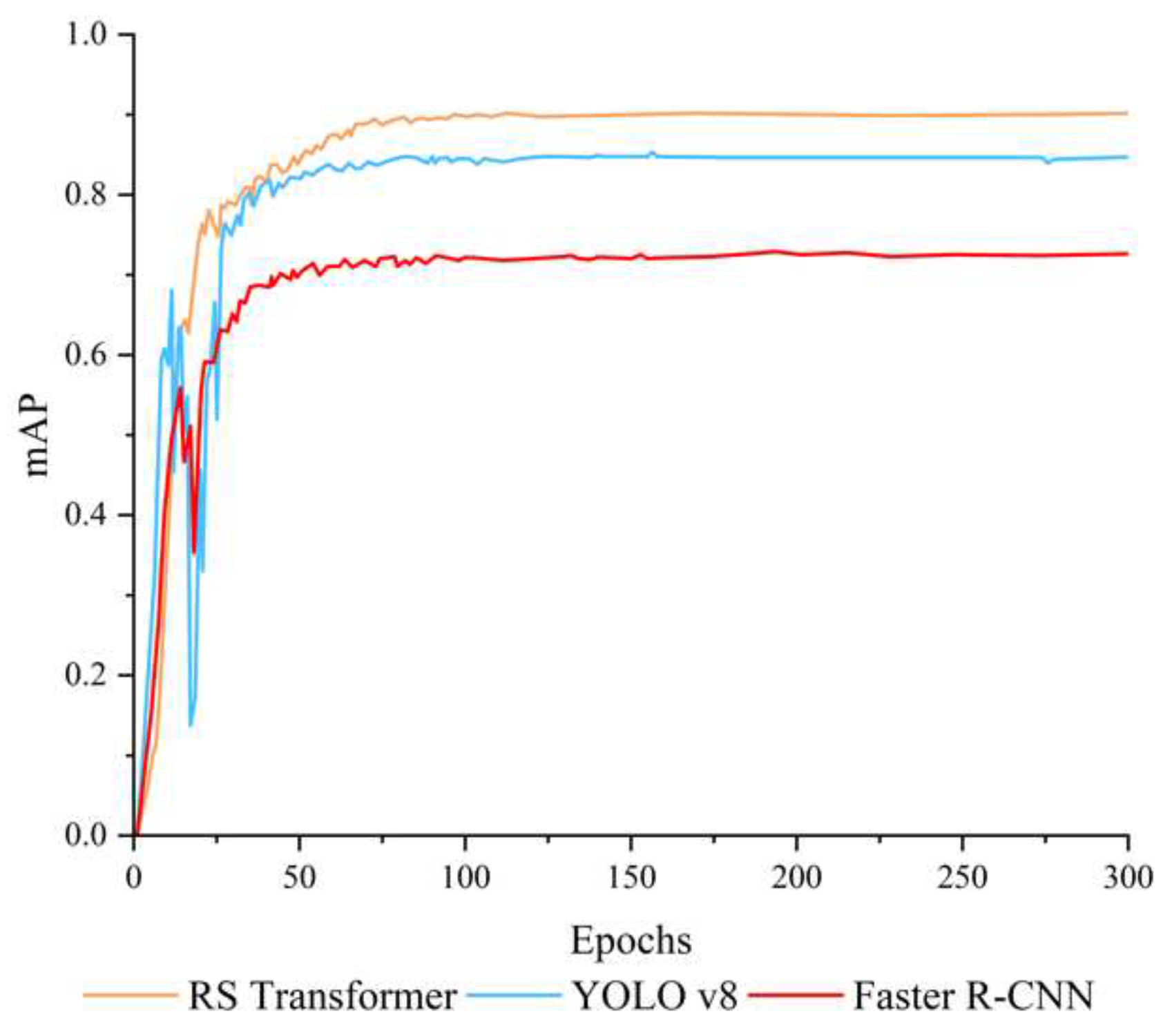
The contrast in mAP is visually presented in
Figure 11. It is evident that the mAP of the three compared models exhibits an upward trend during the training process, albeit with substantial fluctuations. Conversely, our model's mAP shows a more consistent trajectory, stabilizing at 77.73% approximately after 75 epochs. Subsequently, the RS Transformer model attains its peak performance, achieving a maximum mAP of 90.18%. These findings collectively affirm the stability of the RS Transformer, its capacity to enhance network performance, and its ability to expedite convergence.
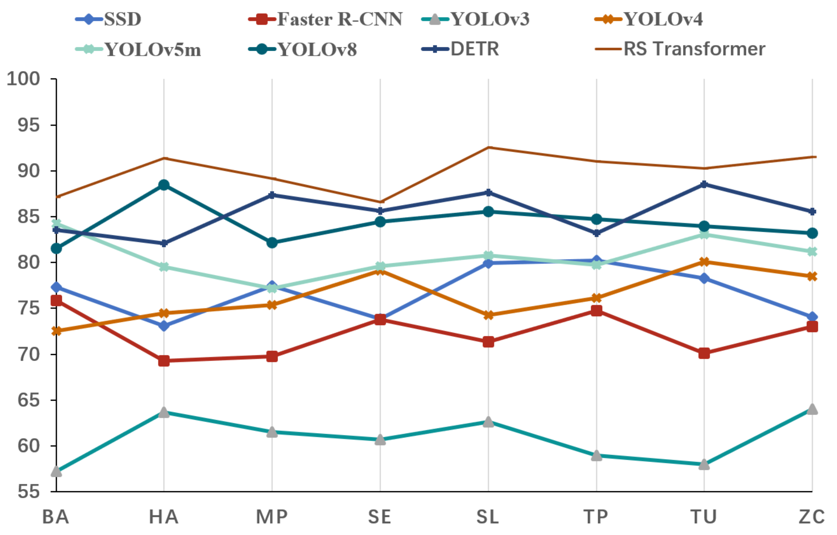
The RS Transformer exhibits a robust capacity for discerning similar pests and demonstrates superior overall performance compared to other models, as detailed in
Table 3(models’ mAP) and illustrated in
Figure 12. Furthermore, in challenging scenarios such as the TU dataset the model maintains a remarkable recognition rate of 90.24%.
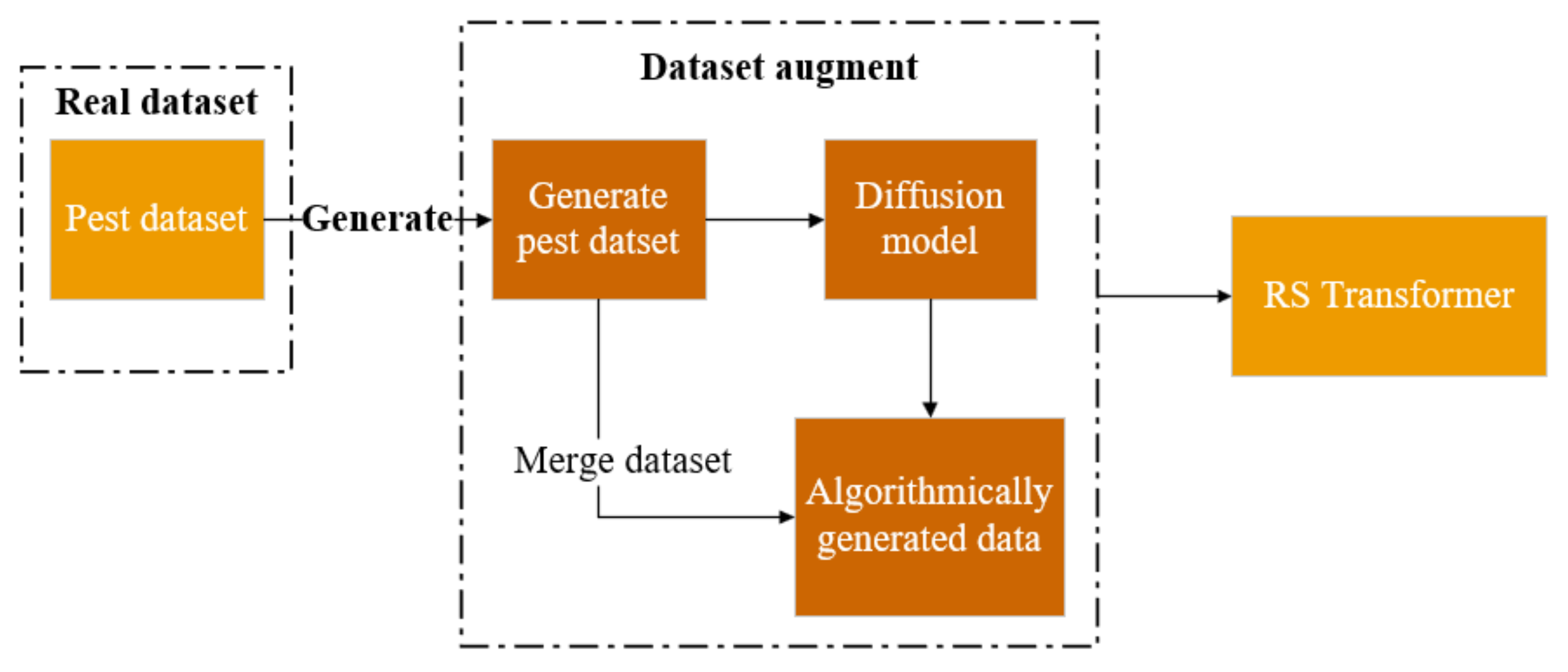
The dataset has been generated using the diffusion model (see
Figure 13), and subsequently, it has been combined at varying proportions of 10%, 20%, 30%, 40%, and 50%. These datasets were then utilized as inputs for the RS Transformer model, followed by rigorous testing procedures, culminating in the presentation of the results in
Table 4.
Applying the RGSDD method to the RS Transformer, it is evident that upon incorporating 30% of the generated data, the model attains its peak performance, resulting in a notable increase of 5.53% in mAP.
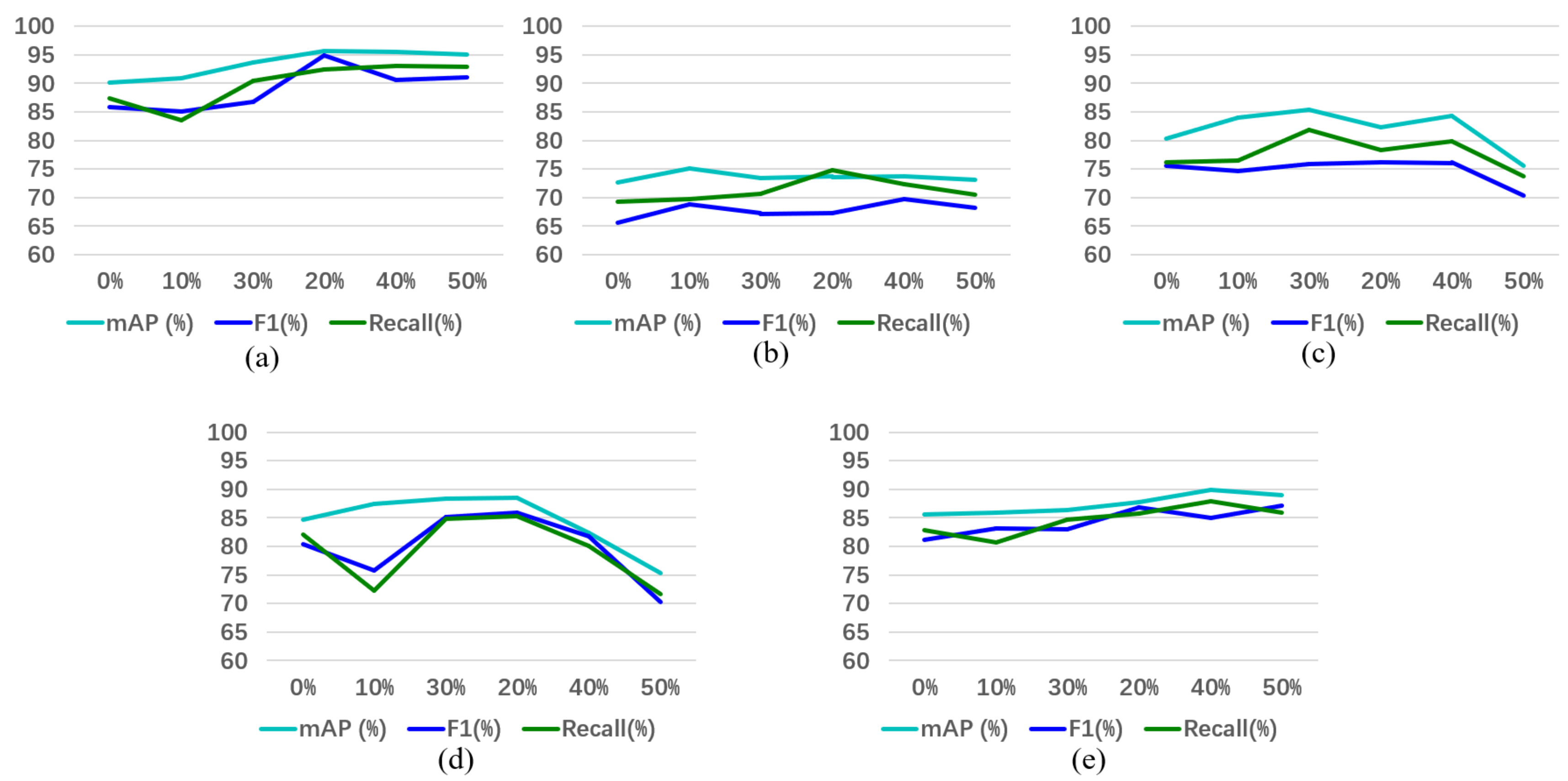
The RGSDD methodology has also been applied to enhance the performance of the Faster R-CNN, YOLOv5m, YOLOv8, and DETR models. The results of these experiments demonstrate that RGSDD contributes positively to model enhancement, as evidenced in
Table 5,
Table 6,
Table 7 and
Table 8.
These data underscore the practical applicability of RGSDD, as visually depicted in
Figure 14. Specifically, in the case of the YOLOv8 model with 30% incorporation, it yielded a substantial 3.79% improvement in mAP. Similarly, for the DETR model with 40% incorporation, there was a noticeable enhancement of 4.36% in mAP. Furthermore, it becomes evident that when 50% of the generated data is included, the model's performance experiences a significant decline. This subset of data appears to introduce interference and is potentially treated as noise to some extent, resulting in adverse effects on model performance.
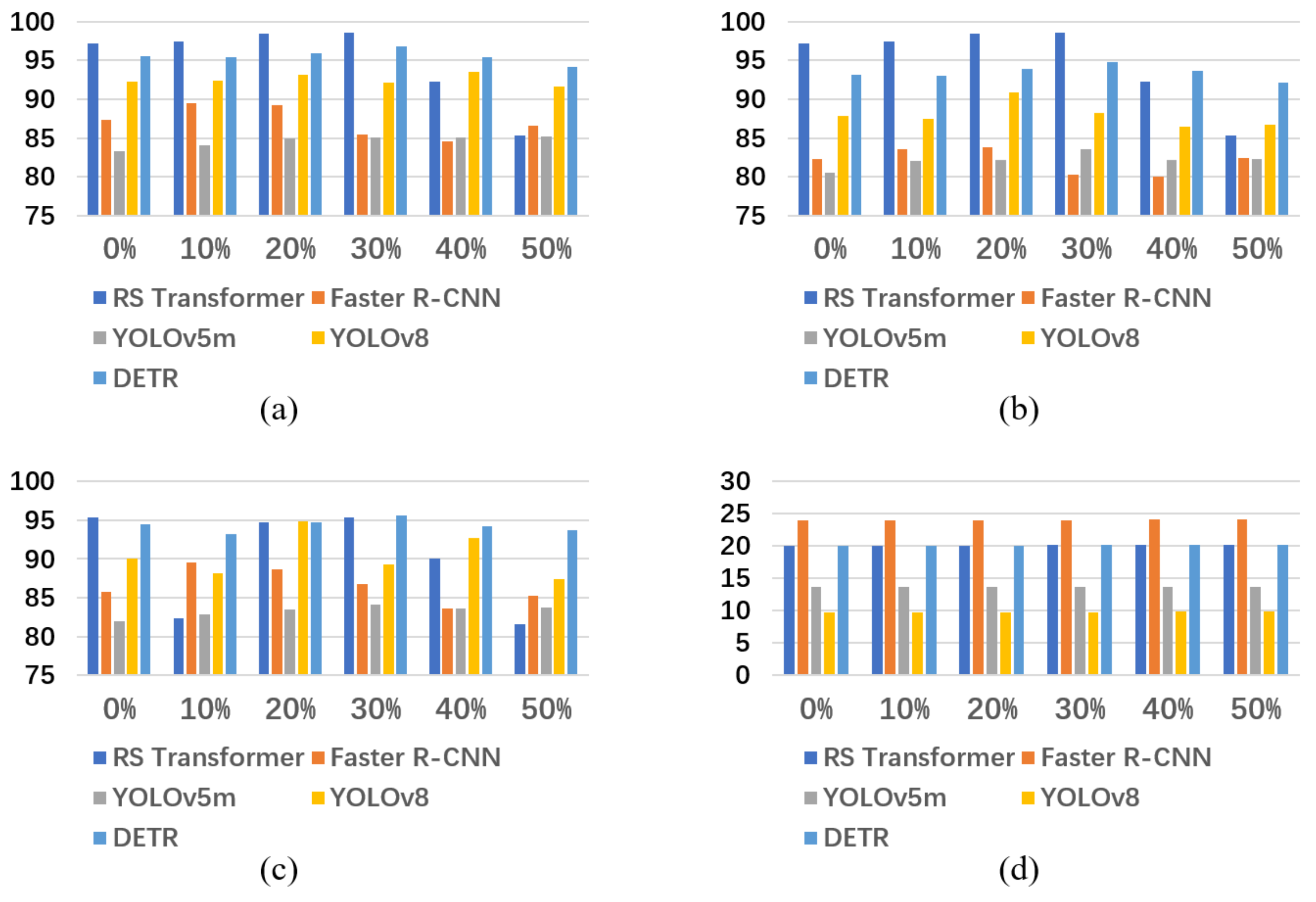
Figure 15 compares the mAP, F1 Score (%) and Recall of different networks, it can be found that RS Transformer is still better than others, even when RGSDD is used. In the optimal value, mAP outperforms Faster R-CNN by 9.29% and YOLOv5m by 4.95 %.
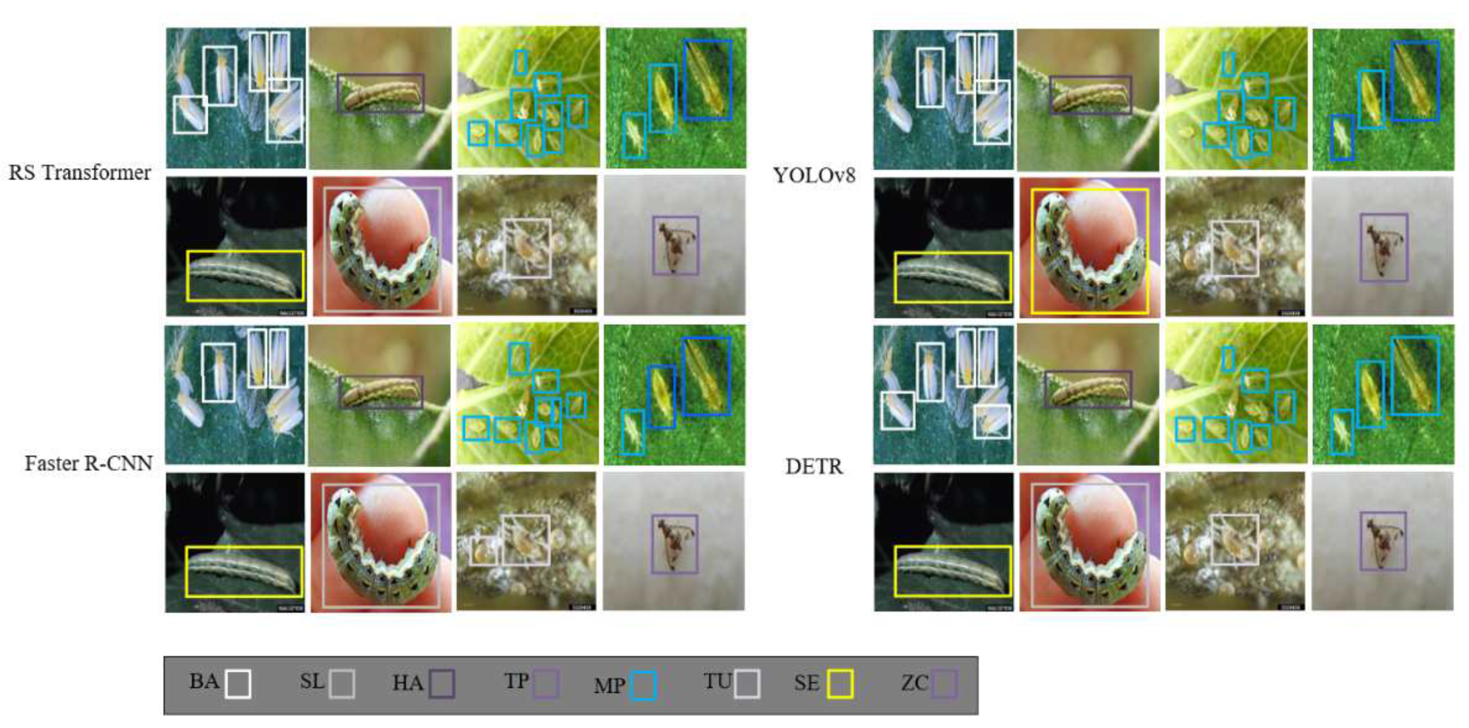
Figure 16 presents the outcomes achieved by the RS Transformer model integrated with RGSDD. Notably, the results highlight RGSDD's exceptional accuracy in effectively identifying multi-scale pests across various species.
5. Conclusions
The Swin Transformer, introduced here as the foundational network for pest detection, represents a pioneering contribution. In conjunction with this innovation, the RS Transformer is developed, building upon the inherent strengths of the R-CNN framework. Furthermore, we employ a diffusion model to create a novel pest dataset, accompanied by introducing an innovative training approach tailored for the Randomly Generated Stable Diffusion Dataset (RGSDD). This approach involves the judicious fusion of synthetic data generated through RGSDD with real data, calibrated as a percentage of the total dataset. Our study comprehensively compares the performance of the RS Transformer and RGSDD against established models including SSD, Faster R-CNN, YOLOv3, YOLOv4, YOLOv5m, YOLOv8, and DETR. The experimental results unequivocally demonstrate the superiority of the RS Transformer and the efficacy of the RGSDD dataset, surpassing prevailing benchmarks. Significantly, our method achieves an optimal balance between accuracy and network characteristics. These findings hold substantial implications for future ecological informatics research, offering fresh insights into the domain of ecological pest and disease control. The presented approach promises to advance the state-of-the-art and contribute to more effective ecological management strategies.
Author Contributions
Conceptualization, L.Z. and T.W.; methodology, L.Z. and L.S.; software, T.W.; validation, T.W.; formal analysis, T.W.; investigation, T.W.; resources, L.Z.; data curation, T.W. and X.W.; writing—original draft preparation, T.W.; writing—review and editing, L.Z. and L.S.; visualization, T.W., X.W.; supervision, L.Z, J.L., Z.L.; project administration, L.Z.; funding acquisition, L.S.; All authors have read and agreed to the published version of the manuscript.
Funding
This work is supported by the National Key Research and Development Program “Industrial Software” Key Special Project(2022YFB3305602), Social Science Planning Foundation of Beijing(20GLC059), Humanities and Social Sciences Planning Fund of the Ministry of Education (22YJA630111, 22YJAZH110).
Institutional Review Board Statement
Not applicable.
Informed Consent Statement
Not applicable.
Data Availability Statement
Not applicable.
Acknowledgments
Thanks for any help in writing this article.
Conflicts of Interest
The authors declare no conflict of interest.
References
- Merle, I.; Hipólito, J.; Requier, F. Towards Integrated Pest and Pollinator Management in Tropical Crops. Current Opinion in Insect Science 2022, 50, 100866. [Google Scholar] [CrossRef]
- Kannan, M.; Bojan, N.; Swaminathan, J.; Zicarelli, G.; Hemalatha, D.; Zhang, Y.; Ramesh, M.; Faggio, C. Nanopesticides in Agricultural Pest Management and Their Environmental Risks: A Review. Int. J. Environ. Sci. Technol. 2023, 20, 10507–10532. [Google Scholar] [CrossRef]
- Bras, A.; Roy, A.; Heckel, D.G.; Anderson, P.; Karlsson Green, K. Pesticide Resistance in Arthropods: Ecology Matters Too. Ecology Letters 2022, 25, 1746–1759. [Google Scholar] [CrossRef]
- Redmon, J.; Farhadi, A. YOLOv3: An Incremental Improvement 2018.
- Bochkovskiy, A.; Wang, C.-Y.; Liao, H.-Y.M. YOLOv4: Optimal Speed and Accuracy of Object Detection 2020.
- Wang, J.; Chen, Y.; Dong, Z.; Gao, M. Improved YOLOv5 Network for Real-Time Multi-Scale Traffic Sign Detection. Neural Comput & Applic 2023, 35, 7853–7865. [Google Scholar] [CrossRef]
- Liu, W.; Anguelov, D.; Erhan, D.; Szegedy, C.; Reed, S.; Fu, C.-Y.; Berg, A.C. SSD: Single Shot MultiBox Detector. In; 2016; Vol. 9905, pp. 21–37.
- Girshick, R. Fast R-CNN 2015.
- Ren, S.; He, K.; Girshick, R.; Sun, J. Faster R-CNN: Towards Real-Time Object Detection with Region Proposal Networks 2016.
- Vaswani, A.; Shazeer, N.; Parmar, N.; Uszkoreit, J.; Jones, L.; Gomez, A.N.; Kaiser, L.; Polosukhin, I. Attention Is All You Need 2017.
- Brasoveanu, A.M.P.; Andonie, R. Visualizing Transformers for NLP: A Brief Survey. In Proceedings of the 2020 24th International Conference Information Visualisation (IV); IEEE: Melbourne, Australia, September, 2020; pp. 270–279. [Google Scholar]
- Dosovitskiy, A.; Beyer, L.; Kolesnikov, A.; Weissenborn, D.; Zhai, X.; Unterthiner, T.; Dehghani, M.; Minderer, M.; Heigold, G.; Gelly, S.; et al. An Image Is Worth 16x16 Words: Transformers for Image Recognition at Scale 2021.
- Liu, Z.; Lin, Y.; Cao, Y.; Hu, H.; Wei, Y.; Zhang, Z.; Lin, S.; Guo, B. Swin Transformer: Hierarchical Vision Transformer Using Shifted Windows 2021.
- Li, W.; Zheng, T.; Yang, Z.; Li, M.; Sun, C.; Yang, X. Classification and Detection of Insects from Field Images Using Deep Learning for Smart Pest Management: A Systematic Review. Ecological Informatics 2021, 66, 101460. [Google Scholar] [CrossRef]
- Sohl-Dickstein, J.; Weiss, E.A.; Maheswaranathan, N.; Ganguli, S. Deep Unsupervised Learning Using Nonequilibrium Thermodynamics 2015.
- Yang, L.; Zhang, Z.; Song, Y.; Hong, S.; Xu, R.; Zhao, Y.; Zhang, W.; Cui, B.; Yang, M.-H. Diffusion Models: A Comprehensive Survey of Methods and Applications 2023.
- Aggarwal, A.; Mittal, M.; Battineni, G. Generative Adversarial Network: An Overview of Theory and Applications. International Journal of Information Management Data Insights 2021, 1, 100004. [Google Scholar] [CrossRef]
- Ho, J.; Jain, A.; Abbeel, P. Denoising Diffusion Probabilistic Models 2020.
- Dhariwal, P.; Nichol, A. Diffusion Models Beat GANs on Image Synthesis.
- Ramesh, A.; Dhariwal, P.; Nichol, A.; Chu, C.; Chen, M. Hierarchical Text-Conditional Image Generation with CLIP Latents 2022.
- Zhu, X.; Su, W.; Lu, L.; Li, B.; Wang, X.; Dai, J. Deformable DETR: Deformable Transformers for End-to-End Object Detection 2021.
- Letourneau, D.K.; Goldstein, B. Pest Damage and Arthropod Community Structure in Organic vs. Conventional Tomato Production in California: Arthropod Community Structure. Journal of Applied Ecology 2001, 38, 557–570. [Google Scholar] [CrossRef]
- Borji, A. Generated Faces in the Wild: Quantitative Comparison of Stable Diffusion, Midjourney and DALL-E 2 2022.
- Cubuk, E.D.; Zoph, B.; Mane, D.; Vasudevan, V.; Le, Q.V. AutoAugment: Learning Augmentation Strategies From Data. In Proceedings of the 2019 IEEE/CVF Conference on Computer Vision and Pattern Recognition (CVPR); IEEE: Long Beach, CA, USA, June, 2019; pp. 113–123. [Google Scholar]
- Thenmozhi, K.; Srinivasulu Reddy, U. Crop Pest Classification Based on Deep Convolutional Neural Network and Transfer Learning. Computers and Electronics in Agriculture 2019, 164, 104906. [Google Scholar] [CrossRef]
- Gong, T.; Chen, K.; Wang, X.; Chu, Q.; Zhu, F.; Lin, D.; Yu, N.; Feng, H. Temporal ROI Align for Video Object Recognition. AAAI 2021, 35, 1442–1450. [Google Scholar] [CrossRef]
- Carion, N.; Massa, F.; Synnaeve, G.; Usunier, N.; Kirillov, A.; Zagoruyko, S. End-to-End Object Detection with Transformers. In Computer Vision – ECCV 2020; Vedaldi, A., Bischof, H., Brox, T., Frahm, J.-M., Eds.; Lecture Notes in Computer Science; Springer International Publishing: Cham, 2020; Volume 12346, pp. 213–229. ISBN 978-3-030-58451-1. [Google Scholar]
Figure 2.
The diffusion processes.
Figure 2.
The diffusion processes.
Figure 3.
The framework of the diffusion model.
Figure 3.
The framework of the diffusion model.
Figure 4.
The generated pest dataset.
Figure 4.
The generated pest dataset.
Figure 5.
Structure diagram of RS Transformer.
Figure 5.
Structure diagram of RS Transformer.
Figure 6.
Structure diagram of RS Transformer.
Figure 6.
Structure diagram of RS Transformer.
Figure 7.
Sample diagram of a hierarchy of small patch size.
Figure 7.
Sample diagram of a hierarchy of small patch size.
Figure 8.
FPN structure diagram.
Figure 8.
FPN structure diagram.
Figure 9.
RPN working principle diagram.
Figure 9.
RPN working principle diagram.
Figure 10.
ROI Align diagram.
Figure 10.
ROI Align diagram.
Figure 11.
Comparisons of mAP.
Figure 11.
Comparisons of mAP.
Figure 12.
Comparisons of mAP to identify similar pests.
Figure 12.
Comparisons of mAP to identify similar pests.
Figure 13.
Mixed data model diagram.
Figure 13.
Mixed data model diagram.
Figure 14.
(a) RS Transformer with RGSDD (b) Faster R-CNN with RGSDD (c) YOLOv5m with RGSDD (d) YOLOv8 with RGSDD (e) DETR with RGSDD.
Figure 14.
(a) RS Transformer with RGSDD (b) Faster R-CNN with RGSDD (c) YOLOv5m with RGSDD (d) YOLOv8 with RGSDD (e) DETR with RGSDD.
Figure 15.
(a) mAP (b) F1 Score (c) Recall (d) mDT.
Figure 15.
(a) mAP (b) F1 Score (c) Recall (d) mDT.
Figure 16.
RS transformer, Faster R-CNN, YOLOv8 and DETR output through the RGSDD system.
Figure 16.
RS transformer, Faster R-CNN, YOLOv8 and DETR output through the RGSDD system.
Table 2.
Comparison of different indexes.
Table 2.
Comparison of different indexes.
| Models |
mAP (%) |
𝐹1𝑆𝑐𝑜𝑟𝑒 (%)
|
Recall |
mDT (ms) |
| SSD |
76.91 |
67.62 |
70.12 |
22.9 |
| Faster R-CNN |
72.65 |
65.57 |
69.31 |
24.5 |
| YOLOv3 |
60.38 |
52.38 |
57.78 |
17.7 |
| YOLOv4 |
76.31 |
69.55 |
74.97 |
10.7 |
| YOLOv5m |
80.29 |
75.58 |
79.14 |
13.6 |
| YOLOv8 |
84.72 |
80.32 |
82.11 |
9.8 |
| DETR |
85.56 |
81.18 |
82.82 |
19.2 |
| RS Transformer |
90.18 |
85.89 |
87.31 |
20.1 |
Table 3.
Comparison of different mAP indexes.
Table 3.
Comparison of different mAP indexes.
| Models |
BA |
HA |
MP |
SE |
SL |
TP |
TU |
ZC |
| SSD |
77.29 |
73.12 |
77.48 |
73.88 |
79.91 |
80.21 |
78.26 |
74.08 |
| Faster R-CNN |
75.89 |
69.26 |
69.76 |
73.81 |
71.33 |
74.75 |
70.10 |
73.02 |
| YOLOv3 |
57.20 |
63.69 |
61.51 |
60.66 |
62.63 |
58.93 |
58.00 |
64.05 |
| YOLOv4 |
72.55 |
74.47 |
75.40 |
79.11 |
74.24 |
76.13 |
80.05 |
78.51 |
| YOLOv5m |
84.22 |
79.51 |
77.17 |
79.57 |
80.79 |
79.73 |
83.06 |
81.16 |
| YOLOv8 |
81.53 |
88.45 |
82.18 |
84.44 |
85.56 |
84.73 |
83.95 |
83.21 |
| DETR |
83.53 |
82.07 |
87.33 |
85.61 |
87.62 |
83.23 |
88.52 |
85.52 |
| RS Transformer |
87.13 |
91.36 |
89.13 |
86.61 |
92.53 |
91.04 |
90.24 |
91.52 |
Table 4.
RGSDD using in RS Transformer.
Table 4.
RGSDD using in RS Transformer.
| Models |
percentage |
mAP (%) |
F1 Score (%) |
Recall (%) |
mDT (ms) |
| RS Transformer |
0% |
90.18 |
85.89 |
87.31 |
20.1 |
| 10% |
90.98 |
85.13 |
83.53 |
20.1 |
| 20% |
93.64 |
86.75 |
90.42 |
20.1 |
| 30% |
95.71 |
94.82 |
92.47 |
20.2 |
| 40% |
95.56 |
90.67 |
93.10 |
20.2 |
| 50% |
94.98 |
91.03 |
93.06 |
20.2 |
Table 5.
RGSDD using Faster R-CNN.
Table 5.
RGSDD using Faster R-CNN.
| Models |
percentage |
mAP (%) |
F1 Score (%) |
Recall (%) |
mDT (ms) |
| Faster R-CNN |
0% |
72.65 |
65.57 |
69.31 |
24 |
| 10% |
75.07 |
68.83 |
69.73 |
24 |
| 20% |
73.47 |
67.26 |
70.62 |
24 |
| 30% |
73.72 |
67.37 |
74.84 |
24 |
| 40% |
71.80 |
69.78 |
72.39 |
24.1 |
| 50% |
73.13 |
68.29 |
70.47 |
24.1 |
Table 6.
RGSDD using YOLOv5m.
Table 6.
RGSDD using YOLOv5m.
| Models |
percentage |
mAP (%) |
F1 Score (%) |
Recall (%) |
mDT (ms) |
| YOLOv5m |
0% |
80.29 |
75.58 |
76.14 |
13.6 |
| 10% |
83.96 |
74.72 |
76.48 |
13.6 |
| 20% |
85.43 |
75.90 |
81.91 |
13.6 |
| 30% |
82.31 |
76.24 |
78.38 |
13.6 |
| 40% |
84.37 |
76.12 |
79.82 |
13.7 |
| 50% |
75.53 |
70.41 |
73.76 |
13.7 |
Table 7.
RGSDD using YOLOv8.
Table 7.
RGSDD using YOLOv8.
| Models |
percentage |
mAP (%) |
F1 Score (%) |
Recall (%) |
mDT (ms) |
| YOLOv8 |
0% |
84.72 |
80.32 |
82.11 |
9.8 |
| 10% |
87.38 |
75.77 |
72.31 |
9.8 |
| 20% |
88.42 |
85.17 |
84.78 |
9.8 |
| 30% |
88.51 |
85.89 |
85.31 |
9.8 |
| 40% |
82.32 |
81.76 |
80.11 |
9.9 |
| 50% |
75.35 |
70.32 |
71.58 |
9.9 |
Table 8.
RGSDD using DETR. Civilization starts from me to create a civilized city
Table 8.
RGSDD using DETR. Civilization starts from me to create a civilized city
| Models |
percentage |
mAP (%) |
F1 Score (%) |
Recall (%) |
mDT (ms) |
| DETR |
0% |
85.56 |
81.18 |
82.82 |
20.1 |
| 10% |
85.94 |
83.10 |
80.62 |
20.1 |
| 20% |
86.37 |
82.99 |
84.67 |
20.1 |
| 30% |
87.71 |
86.75 |
85.72 |
20.2 |
| 40% |
89.92 |
85.02 |
87.89 |
20.2 |
| 50% |
88.90 |
87.19 |
85.97 |
20.2 |
|
Disclaimer/Publisher’s Note: The statements, opinions and data contained in all publications are solely those of the individual author(s) and contributor(s) and not of MDPI and/or the editor(s). MDPI and/or the editor(s) disclaim responsibility for any injury to people or property resulting from any ideas, methods, instructions or products referred to in the content. |
© 2023 by the authors. Licensee MDPI, Basel, Switzerland. This article is an open access article distributed under the terms and conditions of the Creative Commons Attribution (CC BY) license (http://creativecommons.org/licenses/by/4.0/).
