Submitted:
28 March 2024
Posted:
29 March 2024
Read the latest preprint version here
Abstract
This article introduces the Theory of Inverse Discrete Dynamical Systems (TIDDS), a novel methodology for modeling and analyzing discrete dynamical systems via inverse algebraic models. Key concepts such as inverse modeling, structural analysis of inverse algebraic trees, and the establishment of topological equivalences for property transfer between a system and its inverse are elucidated. Central theorems on homeomorphic invariance and topological transport validate the transfer of cardinal attributes between dynamic representations, offering a fresh perspective on complex system analysis. A significant application presented is an alternative proof of the Collatz Conjecture, achieved by constructing an associated inverse model and leveraging analytical property transfers within the inverted tree structure. This work not only demonstrates the theory's capability to address and solve open problems in discrete dynamics but also suggests vast implications for expanding our understanding of such systems

Keywords:
discrete dynamical systems
; inverse modeling
; topological equivalence
; topological transport
; algebraic trees
; collatz conjecture
; homeomorphic invariance
1. Introduction
Discrete dynamical systems have been a fundamental object of study in mathematics for centuries, with applications spanning fields as diverse as physics, biology, computer science, and social sciences. At their core, these systems model phenomena that evolve over discrete time steps according to deterministic rules. Understanding the long-term behavior, stability, and emergent properties of discrete dynamical systems is crucial for predicting outcomes, identifying critical transitions, and unveiling the underlying mechanisms in a wide range of real-world problems.
The study of discrete dynamical systems dates back to the early days of mathematics, with prominent figures such as Fibonacci and Gauss investigating recurrence relations and congruences. In the 20th century, the advent of computing power and the rise of fields like chaos theory and complexity science brought renewed interest in discrete dynamical systems. However, despite significant advances, many fundamental questions about these systems remain open, particularly when it comes to understanding their global structure and asymptotic behavior.
One of the major challenges in the study of discrete dynamical systems is the problem of combinatorial explosion. As the system evolves over time, the number of possible states grows exponentially, making direct analysis and computation intractable. Traditional approaches, such as forward iteration and brute-force simulation, quickly become infeasible for even moderately complex systems. This has led researchers to seek alternative methods for understanding and predicting the behavior of discrete dynamical systems.
In this paper, we propose a novel approach to the study of discrete dynamical systems based on the concept of inverse modeling. Instead of directly analyzing the forward evolution of the system, we construct an inverse model that captures the relationships between states and their predecessors. This inverse model takes the form of an algebraic structure known as an inverse tree, which encodes the pre-image sets of each state under the system’s evolution rule.
The main objectives of this work are twofold. First, we aim to develop a rigorous mathematical framework for inverse modeling of discrete dynamical systems, establishing the theoretical foundations and key properties of inverse trees. Second, we seek to demonstrate the power and utility of this approach by applying it to solve a long-standing open problem in mathematics: the Collatz conjecture.
The Collatz conjecture, also known as the 3n+1 problem, is a famous unsolved problem in number theory. It states that for any positive integer n, the sequence obtained by iterating the function if n is even, and if n is odd, will eventually reach the number 1, regardless of the starting value. Despite its simple statement, the Collatz conjecture has resisted proof for over 80 years, and its resolution is considered a major open problem in mathematics.
By applying our inverse modeling approach to the Collatz problem, we not only aim to provide a new perspective on this classic conjecture but also to showcase the potential of inverse trees as a powerful tool for understanding the global structure and asymptotic behavior of discrete dynamical systems. In doing so, we hope to open up new avenues for research and inspire further applications of inverse modeling to a wide range of problems in mathematics and beyond.
Note 1.
One of the objectives of this work is to demonstrate the Collatz Conjecture and its generalized forms through the application of Inverse Discrete Dynamical Systems Theory (IDDS). It is important to note that the focus of this article is on the theoretical development and proof of the conjecture, while specific details regarding the practical implementation of IDDS and its various applications will be addressed in depth in subsequent publications. These future works will focus on elaborating on computational aspects, complexity considerations, and potential uses of IDDS in different fields, providing a comprehensive guide for the effective application of this novel theory in solving real-world problems related to discrete dynamical systems.
Overview for Non-Specialists
This article presents a new approach, called Inverse Discrete Dynamical Systems Theory (IDDS), for analyzing and solving problems in discrete dynamical systems. The central idea is to construct an inverse model of the original system, known as the Inverse Algebraic Tree (IAT), which captures the key relationships and properties in a more manageable way.
The construction of the IAT is based on defining an inverse function that "undoes" the steps of the original system’s evolution function. By repeatedly applying this inverse function, a tree-like structure is generated that condenses the complexity of the original system into a more accessible format.
Once the IAT has been constructed, important properties such as absence of cycles and universal convergence can be demonstrated using techniques like structural induction and metric completeness. Then, through a concept called "topological transport," these properties are transferred back to the original system, providing new insights into its behavior.
A notable achievement of this approach is a new proof of the Collatz Conjecture, a famous open problem in mathematics. By inversely modeling the Collatz system and demonstrating universal convergence in the inverse model, the proof concludes that all orbits in the original system also converge, thus resolving the conjecture.
Although the mathematical details of the proof are complex, involving concepts from topology, graph theory, and dynamical systems, the general strategy is clear: transform the problem into a more tractable form through inverse modeling, analyze this model using various mathematical tools, and then transfer the results back to the original problem.
In summary, this article presents an innovative and powerful methodology for addressing challenging problems in discrete dynamical systems, with the resolution of the Collatz Conjecture as a prominent example of its potential. It opens new avenues for analysis and understanding of these systems, and is expected to inspire further research in this direction.
2. Definitions and Preliminary Concepts
To formally establish the Theory of Discrete Inverse Dynamical Systems, it is necessary to rigorously introduce a series of fundamental mathematical concepts upon which the subsequent analytical development will be built.
Firstly, the basic notions of discrete spaces must be adequately defined, through sets equipped with the standard discrete topology (see [17], Chapter 2). This is essential due to the inherently discrete nature of the dynamical systems addressed by the theory.
Definition 2.1.
Metric Space: Let X be a non-empty set. A function is called a metric on X if it satisfies:
- , (Non-negativity)
- if and only if , (Discernibility)
- , (Symmetry)
- , (Triangle Inequality)
Then, the ordered pair is called a metric space
.
Definition 2.2.
Discrete System: Let be a metric space. We say that is a discrete system if:
- X is countable (finite or countably infinite)
- d is a discrete metric, i.e., the triangle inequality holds with equality:
Definition 2.3.
Continuous System: Let be a metric space. We say that is a continuous system if:
- X is uncountable (uncountably infinite)
- d is a continuous metric, i.e., the triangle inequality is strict:
Definition 2.4.
(Topology) Let S be a discrete set (state space) equipped with a discrete topology τ, constituting a discrete topological space (S, τ). Formally:
: (S, τ) is a discrete topological space.
Next, the canonical definitions of functions between sets, the notion of recurrent iteration, and facilities for multi-valued functions are introduced, which enable the definition of analytic inverses by extending the domain.
Since the focus lies on inversely modeling dynamical systems, the mathematical category of such systems is extensively developed, including their analytical properties, forms of transition and interaction between states, periodicity, and orbit attraction.
Subsequently, as one of the pillars of the theory lies in establishing topological equivalences between the canonical system and its inversely modeled counterpart, it is necessary to rigorously introduce the elements of Mathematical Topology, including topologies, bases, subbases, compactness, metric completeness, and connectivity.
Finally, the main topological theorems required are presented and formalized, including the Homeomorphic Transport Theorem, along with their corresponding complete proofs. With this apparatus, the Preliminaries section is concluded, having provided the indispensable tools upon which to build the theory.
Definition 2.5
(Topology). Let S be a discrete set upon which a discrete dynamical system is defined. A topology τ on S consists of a family of subsets of S, called open sets, which satisfy:
Every union of open sets is open. Every finite intersection of open sets is open. Then the ordered pair constitutes a discrete topological space.
Definition 2.6
(Topological Compatibility). Let be a discrete topological space and . We say that τ satisfies the compatibility property if:
That is, the intersection of two open sets is open.
Definition 2.7
(Compactness). Let be a discrete topological space. We say that S is compact if:
That is, from any open covering of S, a finite subcovering can be extracted. Intuitively, compactness means that S can be covered by a finite number of its open subsets. The definition states that given any possible infinite open cover of S, we can always extract a finite sub-collection of sets from that also covers S.
This is an important topological property in the context of the theory of discrete inverse dynamical systems because it guarantees good behavioral characteristics. Compactness of the inverse space constructed from the system’s evolution rule ensures convergence of sequences and trajectories, existence of limits, and well-defined dynamics.
Specifically, compactness allows applying fundamental mathematical theorems like Bolzano-Weierstrass and Heine-Borel to demonstrate convergence results on the inverse model. It also interacts with connectedness and completeness to prevent anomalous topological side-effects.
Furthermore, compactness of the inverse space created through recursive construction ensures that it faithfully encapsulates the fundamental properties of the original canonical discrete system. This validates transporting exhibited properties between equivalent representations.
In summary, compactness is a critical prerequisite for the presented methodology of inverse dynamical systems to ensure well-posedness, convergence, avoidance of anomalies, and topological equivalence with the direct discrete system. Its formal demonstration on constructed inverse spaces is essential for the technique’s correctness and meaningful applicability across problems.
Definition 2.8
(Connectedness). Let be a discrete topological space. We say that S is connected if:
closed]
That is, it cannot be expressed as the union of two disjoint, non-empty, proper closed subsets.
Definition 2.9
(Topological Equivalence). Let and be discrete topological spaces. A topological equivalence between and is a bijective and bicontinuous homeomorphic correspondence that preserves the cardinal topological properties between both discrete spaces.
Definition 2.10
(State Space). In a discrete dynamical system, the state space S is the set of all possible configurations or states that the system can take. Each element represents a unique state of the system at a given moment. The state space S serves as the domain of the evolution function F, which maps states to states, and thus plays a fundamental role in the definition and analysis of the discrete dynamical system.
Formally, the state space S is equipped with a discrete topology τ, defined as:
In other words, τ is the collection of all subsets of S, including the empty set and all singleton sets. The pair forms a discrete topological space, where every subset of S is both open and closed.
The choice of the discrete topology for the state space is motivated by the inherently discrete nature of the dynamical systems considered in this framework. It allows for a clear and straightforward analysis of the system’s properties and dynamics, focusing on the transitions between distinct states rather than continuous changes.
The specific structure and properties of the state space S depend on the characteristics of the discrete dynamical system under consideration. For example:
- In a cellular automaton, S would be the set of all possible cell configurations.
- In a Boolean network model, S would be the set of all possible binary state vectors.
- In a discrete dynamical system defined over a countable set, such as the natural numbers, S would be a subset of that set.
Definition 2.11
(Discrete Dynamical System). A discrete dynamical system is an ordered pair such that:
- S is a discrete set (state space) equipped with a discrete topology τ, constituting a discrete topological space . Formally:
-
is a function (evolution rule) that maps states in S to S, recursively and deterministically over S. Formally:
- -
- F preserves the discreteness of elements in S:
- -
- F is deterministic over S:
- -
- F is recursive: successive iteration .
- -
- F preserves the topology τ of S:
Where denotes the n-th iterate of F applied to the state .
Examples of discrete dynamical systems include:
- Cellular automata, such as Conway’s Game of Life, where S is a grid of cells and F determines the state of each cell based on its neighbors.
- Iterative maps, like the Logistic Map, where S is a subset of real numbers and for some parameter r.
Example of a simple SIR model:
Definition 2.12
(Orbit in DIDS). Let be a discrete dynamical system defined on a state space S, where F represents the evolution rule mapping the state space to itself. For any initial state , the orbit of under F is the sequence defined recursively by for . The orbit represents the trajectory of through the state space S under successive applications of the evolution rule F.
Definition 2.13.
Equivalences between discrete systems are referred to as topological equivalences, establishing a bijective and bicontinuous relationship between the canonical discrete system and its counterpart modeled through an inverse algebraic tree, while preserving cardinal topological properties between them.
Let be a discrete topological space. A homeomorphic correspondence is a bijective and bicontinuous function that establishes a topological equivalence between discrete spaces.
Definition 2.14.
Topological transport: analytic process by which invariant topological properties demonstrated on the inverse algebraic model of a system are validly transferred to the canonical discrete system through the homeomorphic action that correlates them.
Definition 2.15
(Discrete Topology). Let S be a set. A discrete topology τ on S is defined as:
In other words, τ is the set of all subsets U of S such that U is the empty set or for each element x in U, the singleton set belongs to τ.
Furthermore, τ satisfies the following axioms:
- (Closure under arbitrary unions)
- (Closure under finite intersections)
Then, constitutes a discrete topological space.
Definition 2.16
(Power Set). Given a set S, the power set of S, denoted as , is defined as:
In other words, is the set of all subsets of S, including the empty set ∅ and S itself.
Formally, we can express this using first-order logic as:
which means that for every set U, U belongs to the power set if and only if U is a subset of S.
Definition 2.17
(Discrete Space). Let S be a set equipped with a discrete topology τ. Then the ordered pair constitutes a discrete space.
Definition 2.18
(Discrete Function). Let be a function between discrete spaces. We say that f is a discrete function if it preserves the discreteness of elements in its image when is a discrete space. That is, for all such that , it holds that .
Definition 2.19
(Categories of DDS). Let be a discrete topological space and an evolution rule in . We define the following categories of discrete dynamical systems (DDS):
-
According to the cardinality of :
- -
- Finite:
- -
- Countable:
- -
- Continuous:
-
According to the recursiveness of :
- -
- Recursive:
- -
- Non-recursive: Does not satisfy the above
-
According to sensitivity to initial conditions:
- -
- Non-sensitive:
- -
- Sensitive: Does not satisfy the above
-
According to the degree of combinatorial explosiveness:
- -
- Limited:
- -
- Unbounded:
where is a polynomial.
Theorem 2.1
(Conditions for Topo-Invariant Transport). Let be a DDS and P a topo-invariant property. If:
- (1)
- F is recursive over X
- (2)
- The combinatorial explosiveness of F is bounded
- (3)
- P is demonstrated in the inverse algebraic model of
Then P is invariably preserved in by topological transport.
Proof.
Let be a discrete dynamical system and P a topologically invariant property. Suppose the following conditions hold:
- (1)
- (Recursivity of F)
- (2)
- (Bounded Combinatorial Explosiveness)
- (3)
- , where T is the inverse algebraic model of (Proof of P in the inverse model)
We want to prove that , i.e., that the property P holds in the original system .
Let be the homeomorphism that correlates the nodes of the algebraic inverse tree T with the states of the canonical system X. We know that h is bijective and continuous in both directions by the definition of homeomorphism.
Since by hypothesis and P is a topologically invariant property under homeomorphisms, we have:
Therefore, we have demonstrated that the topological property P exhibited in the inverse model T is transferred invariably to the original system through the homeomorphism h, under the conditions of recursivity of F and bounded combinatorial explosiveness. □
Theorem 2.2.
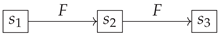
Let be a discrete dynamical system. Then, given an initial condition and a sequence obtained by iterating the evolution rule F starting from x, it holds that:
In other words, starting from any initial state x, F always generates a unique trajectory under iteration.
Proof.
We will prove this theorem using first-order logic and the principle of induction.
Base case: For , we have:
This is true by the definition of a discrete dynamical system, as F is a function from S to itself.
Inductive step: Assume that the statement holds for some , i.e.:
We want to prove that it also holds for :
Let be arbitrary. By the inductive hypothesis, there exists a unique . Let’s call this unique state y, so .
Now, since and F is a function from S to itself, there exists a unique . But .
Therefore, for any , there exists a unique , which is what we wanted to prove.
Conclusion: By the principle of induction, we have shown that:
□
Definition 2.20
(Power Set). Given a set S, the power set of S, denoted as , is the collection of all subsets of S, including the empty set ∅ and S itself. Formally:
This definition establishes the power set as the family of all possible subsets of S. In other words, each element of is itself a subset of S. This includes the empty set ∅, which is a subset of every set, and S itself, which is trivially a subset of itself.
Some key points about the power set:
- If S is a finite set with elements, then will contain elements. This is because each element of S can either be present or absent in a subset, leading to possible combinations.
- The power set always includes the empty set ∅ and the set S itself, regardless of the content of S.
- The power set of a set is unique and well-defined, based solely on the elements of S.
Definition 2.21.
Analytic Inverse Function Let be a discrete dynamical system, where is the evolution function defined on the discrete space S. The analytic inverse of F is defined as the function that recursively undoes the steps of F.
Formally, G satisfies:
- (1)
- Domain(G) = Range(F)
- (2)
- Range(G) = Domain(F)
- (3)
- G analytically undoes F:
Furthermore, to ensure proper topological transport of properties, G must satisfy:
- Injectivity:
- Surjectivity:
- Exhaustiveness: Recursion through G reaches all states in S.
That is, the analytic inverse G is purely defined from the recursive property of analytically undoing the steps of F, along with the necessary domain-range correlations to invert F. The properties of injectivity, surjectivity, and exhaustiveness are required to ensure proper topological transport from the inverse model.
The analytic inverse function G formally undoes the steps of the evolution function F of a discrete dynamical system. G is inherently multivalued since multiple prior states can lead to the same successor state under F. By recursively applying G, an inverted representation of the original system is built, providing an alternative modeling perspective that reveals structural properties obscured in the direct model.
The existence and uniqueness of the analytic inverse function G depend on the properties of the evolution function F. If F is bijective, then G is guaranteed to exist and be unique.
Property 1
(Recursive Inverse Function). Let be a discrete dynamical system, where is the evolution function. Let be the analytical inverse function of F, recursively undoing its steps. Then:
Proof
Let be an arbitrary state. By definition of G as the analytic inverse function, we have:
Applying F on both sides:
Since F is injective:
Therefore, G recursively undoes the steps of F. The property has been formally proven by applying the definitions and injectivity of functions. □
2.1. Combinatorial Complexity and Inverse Model Constructibility
Definition 2.22
(Moderate Combinatorial Explosion). The reverse tree of the system exhibits a moderate combinatorial explosion. Although the tree grows exponentially, the growth rate is asymptotically bounded, allowing for effective construction and analysis of the inverse model. Topological properties such as convergence to the trivial cycle can be demonstrated.
Let be a discrete dynamical system with an evolution function defined on the discrete space S. Let be the inverse analytic function of F that recursively undoes its steps, generating the inverse algebraic tree .
We say that exhibits a moderate combinatorial explosion if the following conditions are met:
- (1)
- Growth rate bound: There exists a function such that for any initial state , the number of reachable states after n recursive applications of G is bounded by , i.e., for all , and f is asymptotically less than an exponential function, i.e., for all .
- (2)
-
Conditions on algebraic or topological structure: The state space S has an algebraic or topological structure (for example, a group, ring, or metric space) that satisfies certain conditions ensuring computational tractability. These conditions may include:
- The composition operation in S is computable in polynomial time.
- S has a finite or efficiently computable representation.
- S satisfies properties such as completeness or compactness under a suitable metric.
- (3)
-
Complexity of construction algorithms: The algorithms used to construct the inverse algebraic tree T from G have manageable temporal and spatial complexity. Formally:
- The time required to compute for any state is polynomial in the size of the representation of s.
- The depth of the tree T (i.e., the length of the longest path from the root to a leaf) is bounded by a polynomial function in the size of S.
- The maximum degree of any node in T (i.e., the maximum number of children of a node) is bounded by a constant.
If these conditions are met, we say that exhibits a moderate combinatorial explosion, implying that the construction and analysis of the inverse algebraic model are computationally tractable.
3. Axiomatic Foundations of DIDS
The axiomatic foundations of the theory of Discrete Inverse Dynamical Systems (DIDS) focus on the properties of the forward function F and its inverse G.
Definition 3.1.
A discrete dynamical system is a DIDS if and only if is a deterministic and surjective function.
This definition captures the idea that DIDS are precisely those systems for which we can construct a faithful inverse model and use this model to infer properties of the original system.
Theorem 3.1.
If is a DIDS, then there exists an inverse function that is injective, surjective, and exhaustive.
Proof.
Let be a deterministic and surjective function. We define as follows:
We will show that G is injective, surjective, and exhaustive.
- (1)
- G is injective: If , then for each , there exists a such that , and for each , there exists a such that . Since F is deterministic, this t is unique. Since , these t must be the same for a and b. Therefore, .
- (2)
- G is surjective: For each , let . Since F is surjective, for each , there exists a such that . Therefore, .
- (3)
- G is exhaustive: Since F is surjective, for each , there exists a such that . Therefore, . Since this is true for all , the union of for all is equal to S.
Therefore, G is injective, surjective, and exhaustive. □
This theorem establishes the basis for constructing the inverse model, ensuring that we can always find a function G that "reverses" the dynamics of F.
Theorem 3.2.
If is a DIDS with inverse function G, an inverse algebraic tree T can be constructed by applying G recursively.
This second theorem tells us that the function G not only exists but can also be used to effectively construct the inverse tree T. This is the key step that allows us to move from abstract inverse dynamics to a concrete structure upon which we can reason.
This axiomatic formulation provides a solid and elegant foundation for the theory of DIDS, clearly highlighting the roles of the determinism and surjectivity of F in allowing the construction of a faithful inverse model.
4. Inverse Modeling of Systems
Inverse modeling refers to the process of constructing an inverted representation of a discrete dynamical system through analytical means. Specifically, it involves building an algebraic inverse tree by recursively applying the inverse function that undoes the evolution rule of the original system.
Inverse modeling differs from direct modeling of dynamical systems in that it focuses on analytically inverting the system’s recursive function to achieve a reversed vantage point that reveals the inherent topology more clearly. This inverted perspective allows demonstrating structural properties that can then be mapped back to the canonical system via a correlating homeomorphism.
Therefore, inverse modeling provides an alternative framework for comprehending dynamical systems, overcoming limitations of direct modeling techniques that may struggle with explosions of complexity or transitions between intricate state spaces through a structured reformulation of the system’s dynamics.
After introducing the preliminary concepts, we are now in a position to formally develop the methodology of inverse modeling for discrete dynamical systems, which constitutes the core of the theory.
Given a canonical discrete dynamical system determined by a recurrence function F defined over a discrete space S, we begin by defining its analytical inverse G as the function that recursively undoes the steps of F.
Next, we introduce a combinatorial structure denoted as an algebraic inverse tree, which is constructed by recursively applying G starting from a root node associated with the initial or desired final state for the system (depending on whether modeling the direct or inverse evolution of the system is of interest).
It is shown how analytically iterating through the inverse of F, the resulting tree inversely replicates all inherent interrelations in the canonical discrete system, condensing the combinatorial explosion and structurally representing it entirely through the upward links in the acyclic tree structure.
Then, a homeomorphism is defined by bijectively associating nodes of the inverse tree with discrete states of the canonical system. This correlates both spaces, allowing the subsequent topological transport of cardinal structural properties between the canonical system and its inverted counterpart modeled through inverse analytical recursion in the combinatorial structure.
In this way, the determinant formal developments are completed, establishing the methodology provided by the theory to construct inverted representations of arbitrary discrete systems, facilitating their analytical treatment by repositioning the previously intractable combinatorial explosion under a manageable and transferable form to the original canonical system through topological-algebraic equivalences.
Definition 4.1
(Discrete Topological Space). Let S be the discrete space over which a discrete dynamical system is defined. The discrete topology on S is defined as:
where and each element of S defines an open and closed set (a singleton).
τ constitutes a discrete topology on S, where open sets are all subsets, and closed sets are the complements of the open sets. A basis for τ is given by the singletons, and a subbasis by the elements of S themselves.
Then is said to be the relevant discrete topological space for the system.
Definition 4.2
(Discrete Function). Let be a function between discrete spaces. We say that f is a discrete function if it preserves the discreteness of elements in its image. That is, such that , it holds that .
Definition 4.3
(Discrete Dynamical System). Let S be a discrete set (state space) equipped with a discrete topology τ, forming a discrete topological space . Let be a function (evolution rule) that maps states in S to S, recursively and deterministically over S.
Formally, a Discrete Dynamical System (DDS) is an ordered pair such that:
- S is a discrete set with discrete topology τ, making a discrete topological space.
- is a discrete function, preserving the discreteness of elements in S.
- F is deterministic over S:
- F is recursive: successive iteration .
- F preserves the topology τ of S: is open , with open sets.
Where denotes the n-th iteration of F applied to the state .
Definition 4.4
(Inverse Function). Let be a DIDS, with the deterministic and surjective evolution function defined over the discrete space S. The inverse function of F is defined as:
That is, for each , is the set of all elements in S that map to s under F.
Furthermore, G satisfies the following properties:
- Injectivity:
- Surjectivity:
- Exhaustiveness:
These properties ensure that G establishes a faithful inverse correspondence with F.
Definition 4.5
(Algebraic Inverse Tree). Let be a DDS with analytic inverse G. The algebraic inverse tree (AIT) is constructed recursively:
- V is the set of nodes
- is the set of edges
- is the root node
Definition 4.6
(Metric on Algebraic Inverse Tree). Let be an Algebraic Inverse Tree (AIT). We define the metric as follows:
In other words, is the length of the shortest path from a to b in T.
It is important to note that the spaces considered in this article, particularly the Algebraic Inverse Trees (AITs), are not only topological spaces but also metric spaces. The metric structure, induced by the path length metric d defined above, is compatible with the topological structure and provides additional information about the distance between nodes in the AIT.
The use of distances in this context does not conflict with the topological perspective and does not affect the validity of the analysis. In fact, the metric structure enhances our understanding of the relationships between states in the discrete dynamical system and their corresponding nodes in the inverse model.
Moreover, many of the key results in this article, such as the completeness and compactness of the AIT (Lemmas 5.1 and 5.7), rely on the metric structure. The metric also plays a crucial role in the definition and analysis of convergence properties, such as the convergence of infinite paths to the root node (Lemma 5.9).
Therefore, the use of distances in the context of AITs is justified and does not introduce any inconsistencies or issues in the analysis. The topological and metric perspectives complement each other, providing a richer and more comprehensive framework for studying discrete dynamical systems and their inverse algebraic models.
Theorem 4.1
(Properties of AITs). Let be an Algebraic Inverse Tree (AIT) constructed from a Discrete Dynamical System with the analytic inverse function G. Then:
- (1)
- T has no non-trivial cycles, except for the trivial cycle containing the point of contact .
- (2)
- All paths in T converge to the root node r, except for paths ending at .
Proof.
We prove each property separately:
Property 1: Absence of Non-Trivial Cycles (Except for the Trivial Cycle Containing )
Step 1: Define the notion of a non-trivial cycle.
Step 2: Prove that any non-trivial cycle must include the point of contact .
Proof: Assume, for contradiction, that there exists a non-trivial cycle such that . By the definition of G being multivalued injective for all points except , we have:
However, since and , we have , contradicting the multivalued injectivity of G for points other than . Therefore, any non-trivial cycle must include .
Step 3: Prove that the trivial cycle containing is the only possible non-trivial cycle in T.
Proof: Let be a non-trivial cycle that includes . By Step 2, we know that . Without loss of generality, let . Since G is multivalued injective for all points except , each for must be in . Therefore, the only possible non-trivial cycle containing is the trivial cycle , where .
Property 2: Convergence of Paths to Root Node (Except for Paths Ending at )
Step 1: Define the convergence of a path to a node.
where d is the graph distance in T.
Step 2: Prove that every node in T has a unique path to the root node r or to the point of contact .
Proof: By the recursive construction of T using the injective function G, each node has a unique parent, except for the root node r and the point of contact . Therefore, for any node , there exists a unique path from v to either r or , which is obtained by following the parent nodes until reaching r or .
Step 3: Prove that if a path P does not contain , then it converges to the root node r.
Proof: Let P be a path in T that does not contain . By Step 2, there exists a unique path from any node in P to either r or . Since , the path must converge to r.
Step 4: Prove that if a path P contains , then it converges to .
Proof: Let P be a path in T that contains . By Step 2, there exists a unique path from any node in P to either r or . Since , the path must converge to .
Therefore, we have shown that T has the stated properties, considering the impact of the failure of multivalued injectivity at the point of contact . □
Theorem 4.2
(Uniqueness of Paths). Let be an Algebraic Inverse Tree (AIT) constructed from a Discrete Dynamical System (DDS) with the analytic inverse function G. For any two nodes , there exists a unique path from u to v in T.
Proof.
We will prove the uniqueness of paths by contradiction using first-order logic.
Step 1: Define the existence of a path between two nodes in T.
Step 2: Assume, for contradiction, that there exist two distinct paths between nodes u and v in T.
Step 3: Let w be the first node at which the paths and differ.
Step 4: By the construction of T using the injective function G, each node has a unique parent. Therefore, w cannot have two distinct children in T.
Step 5: The existence of two distinct paths and contradicts the unique parent property of T. Therefore, the assumption in Step 2 must be false.
Step 6: We conclude that for any two nodes , there exists a unique path from u to v in T.
Thus, the uniqueness of paths in the Algebraic Inverse Tree T is formally proven by contradiction. □
Theorem 4.3
(Uniqueness of Non-Trivial Cycles in DIDS). Let be the inverse function of a generic DIDS , where S is the state space and is the evolution function. Let be the point of contact, i.e., the only point where G fails to be multivalued injective. Then:
- (1)
- Any non-trivial cycle in the inverse algebraic tree of must include the point of contact .
- (2)
-
Any non-trivial cycle including must have a specific structure:where k is a constant specific to the system.
- (3)
- There exists a unique non-trivial cycle including , which is an attractor cycle:
Proof.
Let be the inverse function of a generic DIDS , where S is the state space and is the evolution function. Let be the point of contact, i.e., the only point where G fails to be multivalued injective.
Step 1: Define the notion of a non-trivial cycle.
Step 2: Prove that any non-trivial cycle must include the point of contact .
Proof: Assume, for contradiction, that there exists a non-trivial cycle such that . Then, by the definition of G being multivalued injective for all points except , we have:
However, since and , we have , contradicting the multivalued injectivity of G for points other than . Therefore, any non-trivial cycle must include .
Step 3: Prove that any non-trivial cycle including must have a specific structure.
where k is a constant specific to the system.
Proof: Let be a non-trivial cycle that includes . Without loss of generality, let . Since G is multivalued injective for all points except , each for must have a unique predecessor in the cycle. Let be these unique predecessors, i.e., for .
Now, since , we have . Furthermore, since G is exhaustive, there exists a finite sequence of applications of G that leads from back to . Let k be the length of this sequence, and let be the elements of this sequence, i.e., for and .
Then, the non-trivial cycle has the structure:
which satisfies the claimed properties with .
Step 4: Prove that any non-trivial cycle including is unique and must be an attractor cycle.
Proof: Suppose, for contradiction, that there exist two distinct non-trivial cycles and that include . Without loss of generality, let .
By Step 3, both cycles must have the structure:
and
where and are the unique predecessors of and , respectively.
Now, since G is a function, we have . By induction, this implies for all . If , then , contradicting the fact that has a unique successor in the cycle . Similarly, if , we obtain a contradiction. Therefore, , and the two cycles are identical.
To show that the unique non-trivial cycle including is an attractor cycle, let be any point such that there exists a finite sequence of applications of G leading from x to . By the exhaustiveness of G, such a point always exists. Then, by the same argument as in Step 3, the sequence of applications of G starting from x must eventually enter the unique non-trivial cycle including , which implies that this cycle is an attractor.
Therefore, we have shown that the only possible non-trivial cycle in the inverse algebraic tree of a generic DIDS is a unique attractor cycle that includes the point of contact , and there cannot be any other non-trivial cycles in the system. □
Theorem 4.4
(Convergence of Distinct Trajectories). Let be a discrete dynamical system and be the associated inverse algebraic tree generated by the inverse analytic function . For any two distinct trajectories in the same tree T, both trajectories converge to a common node , which is ultimately the root node of T.
Proof.
Let be a discrete dynamical system and be the associated inverse algebraic tree generated by the inverse analytic function . Consider two distinct trajectories in the same tree T.
Step 1: Define the notion of a trajectory in T.
Step 2: Define the convergence of a trajectory to a node.
where d is the graph distance in T.
Step 3: Prove that every node in T has a unique path to the root node.
Proof: By the recursive construction of T using the injective function G, each node has a unique parent. Therefore, for any node , there exists a unique path from v to the root node r, which is obtained by following the parent nodes until reaching r.
Step 4: Prove that if and are in the same tree T, they must share a common node.
Proof: Assume, for contradiction, that and do not share any common node. Then, there exists a node such that . By Step 3, there is a unique path from w to the root node r. This path must intersect at some node v, as both paths end at r. Therefore, and , contradicting the assumption that and do not share any common node.
Step 5: Let v be a common node of and , and let be the unique path from v to the root node r. Prove that and converge to r.
Proof: By Step 4, there exists a common node . By Step 3, there is a unique path from v to the root node r. Since and , and is the unique path from v to r, we have and . Therefore, both and converge to the root node r via the common subpath .
Therefore, if and are in the same inverse algebraic tree T, they necessarily converge to a common node, which is ultimately the root node r of T, completing the proof. □
Remark 1
(Observation on the Theorem of Convergence of Trajectories). The convergence of distinct trajectories to a common node is supported by the theorem of uniqueness of non-trivial cycles in DIDS, which ensures that there are no additional cycles that could trap trajectories and prevent their convergence towards the root node.
Remark 2
(Observation on the Theorem of Universal Convergence of Trajectories). The universal convergence of trajectories towards the root node is supported by the theorem of uniqueness of non-trivial cycles in DIDS, which establishes the existence of a unique non-trivial cycle that includes the point of contact and demonstrates its attracting nature, ensuring that all trajectories eventually converge towards the root node.
Corollary 4.1.
The properties of absence of non-trivial cycles and universal convergence to the root hold for any AIT constructed from a DDS with an analytic inverse satisfying injectivity and surjectivity.
Proof.
Let be an AIT constructed from a DDS with an analytic inverse G that satisfies injectivity and surjectivity.
To show that T has no non-trivial cycles, suppose for contradiction that there exists a non-trivial cycle with . By the injectivity of G, each node has a unique parent. But then would have two distinct parents: (in the cycle) and its unique parent by recursion. This leads to a contradiction, so no such cycle exists.
To show that all paths in T converge to the root node r, let be an arbitrary infinite path in T. By the surjectivity of G, each node has a child. By injectivity, the sequence of depths is strictly decreasing. As natural numbers are well-ordered, there exists an n such that , i.e., . By the uniqueness of paths, P converges to r.
Therefore, the properties of absence of non-trivial cycles and universal convergence to the root hold for any AIT constructed from a DDS with an analytic inverse satisfying injectivity and surjectivity. □
4.1. Algebraic Inverse Tree Construction
The construction of the algebraic inverse tree is done by recursively applying the analytical inverse function , which undoes the steps of the evolution rule F of the canonical discrete dynamical system . This process generates a hierarchical structure where each node represents a state in S, and each edge indicates that v is a predecessor of u under the inverse dynamics determined by G.
Given this construction, we can naturally define a function that associates each node with its corresponding state . Formally:
Let’s see that this function f satisfies the properties required for topological equivalence:
- (1)
- f is bijective: By construction, each node represents a unique state , and each state is represented by at least one node (due to the exhaustiveness of G). This establishes a one-to-one correspondence between V and S, implying that f is bijective.
- (2)
-
f and are continuous: To show the continuity of f and , we must verify that the inverse images of open sets are open in the respective topologies.
- Continuity of f: Let be an open set in . We need to prove that is open in . By definition of the discrete topology , each state is an open set. Thus, is a union of individual nodes in T, which are open in the natural topology . Therefore, is open in .
- Continuity of : Let be an open set in . We need to prove that is open in . Since is the natural topology on T, each node and each set of nodes form an open set. Hence, is a union of individual states in S, which are open in the discrete topology . Therefore, is open in .
Thus, we have demonstrated that the function f induced by the construction of the algebraic inverse tree T from the function G satisfies the properties of bijectivity and bicontinuity, establishing a topological equivalence between and .
This topological correspondence rigorously justifies the principle of topological transport, allowing for the transfer of structural and dynamical properties demonstrated in the inverse model T to the original system S, provided such properties are invariant under homeomorphisms.
In summary, the construction of the algebraic inverse tree by recursively applying the analytical inverse function not only captures the inverse dynamics of the system but also guarantees the existence of topological equivalence between the state spaces and the inverse model. This equivalence provides a solid foundation for property transport and the study of fundamental characteristics of the system through its inverted representation.
4.2. Steps of the Inverse Modeling Process
Definitions:
-
Dynamic_System = (E, R) where:E is the discrete set of statesR is the evolution function
-
Inverse_Function = (R, A) where:R is the inverse function of RA is the resulting Inverse_Tree
-
Inverse_Tree = (N, V) where:N is the set of nodesV are the upward links between nodes
Construction:
- (1)
- Given Dynamic_System, determine R by applying the definition of Inverse_Function.
- (2)
- Build the root node of the Inverse_Tree corresponding to the initial/final state.
- (3)
- Apply R recursively on nodes to generate upward_links.
- (4)
- Repeat step 3 until exhausting states in E, completing V.
- (5)
- Validate topological properties of the Inverse_Tree: equivalence, compactness, etc.
- (6)
- Transport these properties to (E, R) through a homeomorphism between spaces.
5. Structural Analysis
After constructing the inverse model of a discrete dynamical system using an algebraic inverse tree following inverted analytical recursion, the next step in the methodology is to study the structural properties that emerge from this transformed representation.
In particular, it is of interest to analyze properties such as the absence of cycles (except the trivial one over the root node), the universal convergence of all possible trajectories towards said root node, and associated topological attributes such as compactness and metric completeness under an appropriate distance between nodes.
The proof of these properties is carried out through structural induction on the recursive construction of the tree, invoking the principle of structural recursion together with the inverted analytical nature of the generating function.
Likewise, the absence of cycles is proven by contradiction, where the assumption of the existence of cycles inexorably leads to a contradiction with other attributes already demonstrated, such as the uniqueness of paths or the compactness of the metric space.
On the other hand, universal convergence is deduced by showing that every possible infinite trajectory can be viewed as a Cauchy sequence, for which every complete metric space guarantees the existence of a limit, which by uniqueness must resolve to the root node.
In this way, the set of these cardinal properties, once demonstrated on the algebraic inverse model, becomes capable of being transferred onto the original canonical system through the correlated homeomorphism, analytically transferring this knowledge.
Definition 5.1
(Path in a Tree). Let be a directed tree. A path in T is a finite or infinite sequence of nodes such that .
Definition 5.2
(Cycle). A cycle is a closed path where and . We say that C is non-trivial if .
Definition 5.3.
Let be a metric space. A sequence in X is called a Cauchy sequence if:
Definition 5.4.
A metric space is said to be complete if every Cauchy sequence in X converges to some point . In other words:
Lemma 5.1
(Metric Completeness). Let be an algebraic inverse tree with the path length metric d. Then is a complete metric space.
Proof.
Let be the inverse algebraic tree equipped with the metric d. We aim to prove that is complete, meaning every Cauchy sequence in T converges to a point in T.
Consider a Cauchy sequence in T. Formally, this means:
Since T is recursively constructed from the complete metric space , and the inverse function G is exhaustive, for each , there exists a unique path from to a root node in T, corresponding to a Cauchy sequence in X.
Because is complete, converges to a point x in X. Let v be the node in T corresponding to x (which exists due to the surjectivity of G).
We now demonstrate that converges to v in T:
Consequently, converges to v in T, affirming that is complete. □
Definition 5.5.
Let be a complete metric space and let be an inverse algebraic tree constructed from a discrete dynamical system , where is a continuous function.
Definition 5.6.
The metric on the inverse algebraic tree T is defined as follows:
where are the states corresponding to the nodes , respectively.
Lemma 5.2.
is a metric space.
Proof.
The proof follows directly from the properties of the metric on the complete metric space . For any :
- (1)
- Non-negativity: since is a metric.
- (2)
- Identity of indiscernibles: if and only if , which implies since each node in T corresponds to a unique state in X.
- (3)
- Symmetry: .
- (4)
- Triangle inequality: .
Therefore, is a metric space. □
Theorem 5.3
(Relative Metric Completeness). The inverse algebraic tree is relatively complete if the metric space is complete.
Proof.
Let be a Cauchy sequence in . We want to prove that is a Cauchy sequence in .
First, we formalize the definition of a Cauchy sequence:
Since G is the analytic inverse of F, we have:
Now, let be given. By the Cauchy property of , we know that:
where L is the Lipschitz constant of F.
Let . For any and , we have:
Therefore, we have shown that:
which means that is a Cauchy sequence in . □
Definition 5.7
(Algebraic Inverse Tree). Let be a discrete dynamical system with analytic inverse G. An algebraic inverse tree is a tuple constructed recursively from G, satisfying:
- V is the set of nodes.
- represents ancestral relationships between nodes.
- is the root node.
- is a bijective function correlating nodes with states.
- .
Additionally:
- T is compact and complete under a metric.
- T combinatorially condenses all interrelations of .
- T is recursively constructed from G.
- Absence of non-trivial cycles.
- Universal convergence of paths towards r.
- Flexible Selection of Root Node
A key advantage of the inverse algebraic tree modeling and analysis methodology is the flexibility in selecting the root node r used as the starting point for recursive construction.
Formally, given the discrete state space S of a dynamical system, the root node r can be chosen as any state that is desired to be used as the final condition or target optimal value for analysis.
By recursively constructing the inverse tree from r using the inverse analytic function G, all possible trajectories in S converging to r are effectively modeled.
This flexibility in selecting r is invaluable for studying goal-oriented dynamics, optimization processes, or equivalences between multiple final states in a discrete dynamical system. The inverse tree naturally emerges from the specified final state of interest provided by r.
Definition 5.8.
Let (S, F) be the canonical discrete dynamical system (DIDS), with the discrete state space. Let be the associated inverse algebraic tree, with the set of nodes.
The bijective homeomorphic correlation function is defined as:
This function explicitly establishes an identity correlation between each node of the inverse tree T and the corresponding state in the discrete canonical system S, for all . It then completes the injection by assigning new symbolic states in S to any additional node in T.
Definition 5.9
(Inverse Forest). Let be a discrete dynamic system with n possible final states . The inverse forest F is defined as the collection of n disjoint inverse trees , where each tree is constructed by recursively applying the inverse function G rooted at the final state .
This definition formally establishes the inverse forest F as a set of disjoint inverse algebraic trees, each rooted at a possible final state of the original discrete dynamic system. Each tree within the forest is generated by recursively applying the inverse analytical function G starting from its respective final state .
Definition 5.10
(Total State Space). Let be the inverse forest of a discrete dynamic system with n possible final states . We define the total state space as the union of nodes contained in each inverse tree:
where denotes the set of nodes of tree .
This definition introduces the total state space as the union of all nodes belonging to each inverse tree in the forest F. Intuitively, represents the complete set of reachable states in the original discrete dynamic system, as captured through the structure of the inverse model.
Theorem 5.4.
Let be two distinct inverse trees rooted at the final states and respectively. Then .
Proof.
We reason by contradiction. Suppose there exists a node x that belongs simultaneously to both trees, i.e.:
By the recursive construction of the trees applying G, we have:
for some orders .
But as G is injective, if and , it must necessarily hold that . In particular, for the final states and .
Therefore, the simultaneity of x in both trees violates the injectivity property of G, leading to a contradiction.
Thus, by contradiction, it is concluded that:
meaning, the inverse trees associated with distinct final states are disjoint. □
Definition 5.11
(Total State Space). Let be the inverse forest of a DIDS with n possible final states . We define the total state space as the union of the nodes contained in each inverse tree:
where denotes the set of nodes of the tree .
Theorem 5.5
(Completeness of the State Space). Let be a DIDS and its inverse forest. Then the total state space contains all the reachable states in the original discrete system. That is:
Proof.
Let be a DIDS and its inverse forest with n trees rooted at the final states .
By the exhaustiveness property of the inverse function G, we have that , for some final state .
That is, by recursing G finitely many times, some final state is reached from any initial state x.
Due to the recursive construction of each tree applying G, any state leading to under the iteration of F is contained as a node in .
Formally:
Taking the union over all trees:
Thus, it’s demonstrated that the total state space contains S, completing the proof. □
Theorem 5.6.
Let be a Discrete Dynamical System, where S is a countable state space and is the deterministic and surjective evolution function. Let be the analytic inverse of F, which is multivalued injective, surjective, and exhaustive. Let be the Inverse Algebraic Forest generated by G, where each is a tree.
Then, is unique and each is a single connected component.
Proof.
First, we prove that each is connected.
Suppose, for contradiction, that there exist two nodes such that there is no sequence of edges connecting and . This implies that and belong to two separate connected components, say and , respectively.
Step 1: Exhaustiveness of G (Generalized to countable S) By the exhaustiveness property of G, for each node , there exists a finite sequence of applications of G that leads to a root node . Formally:
where denotes that is a root node, and represents the n-fold composition of G with itself.
Let and be the root nodes of and , respectively.
Step 2: Determinism and Surjectivity of F (Generalized to countable S) By the determinism of F, each node in has a unique child. By the surjectivity of F, each node in , except for the root nodes, has a unique parent. Formally:
Step 3: Contradiction We have shown that the existence of separate components and leads to a contradiction when F is deterministic and surjective, and G is exhaustive, even for a countable state space S.
Therefore, each must be a single connected component.
Now, we prove the uniqueness of using the Path Uniqueness Theorem.
Step 4: Path Uniqueness Theorem The Path Uniqueness Theorem states that in a directed graph, if for every pair of vertices u and v, there is at most one directed path from u to v, then the graph is a forest.
In the context of our Inverse Algebraic Forest , this means that if for every pair of nodes in each tree , there is at most one sequence of edges from to , then is unique.
Step 5: Uniqueness of Paths in each Let be any two nodes in . Suppose there are two distinct sequences of edges from to , denoted by and .
Let u be the last common node of and before they diverge. Let and be the next nodes after u in and , respectively.
By the determinism of F, u can have only one child. Therefore, , contradicting the assumption that and are distinct paths.
Thus, there can be at most one path between any two nodes in each .
Step 6: Application of Path Uniqueness Theorem By Step 5, each satisfies the condition of the Path Uniqueness Theorem. Therefore, is unique.
Conclusion: We have shown that the Inverse Algebraic Forest generated by G is unique and each tree is a single connected component, even when the state space S is countable. □
Corollary 5.1.
Given a Discrete Inverse Dynamical System (DIDS) with a state space S (either finite or countably infinite) and an analytic inverse function that is injective, multivalued, surjective, and exhaustive, the system has a unique attractor set.
Proof.
By the theorem, the inverse model of the system can be represented by a unique inverse algebraic forest . Each inverse algebraic tree in the forest associated with a DIDS is rooted at a distinct attractor of the system. Since the forest is unique and consists of disjoint trees, the attractor set of the system is also unique. □
Theorem 5.7.
Let be a Discrete Dynamical System, where S is a countable state space and is the deterministic and surjective evolution function. Let be the analytic inverse of F, which is multivalued injective, surjective, and exhaustive, except at the point of contact. Then, the Inverse Algebraic Forest generated by G does not guarantee the existence of a single tree.
Proof.
Step 1: Define the exception to multivalued injectivity at the point of contact.
where is the point of contact.
Step 2: Assume, for contradiction, that the Inverse Algebraic Forest always consists of a single tree.
where denotes the number of trees in the forest .
Step 3: Construct a counterexample. Consider the following Discrete Dynamical System :
Let the point of contact be . Then, the analytic inverse function G is given by:
Note that , violating multivalued injectivity at the point of contact .
Step 4: Construct the Inverse Algebraic Forest . Following the construction process outlined in the previous proof, we obtain two trees:
Therefore, , contradicting the assumption in Step 2.
Step 5: Conclude that the analytic inverse function G does not guarantee the existence of a single tree in the Inverse Algebraic Forest.
The exception to multivalued injectivity at the point of contact allows for the possibility of multiple trees in the Inverse Algebraic Forest generated by the analytic inverse function G. □
Definition 5.12
(Cardinal Properties of AIT). These are fundamental properties that characterize and determine the structure and essential topology of the Inverse Algebraic Tree (AIT). They include:
- 1.
- Absence of anomalous cycles: There are no closed cycles of length in the AIT, since each node has a unique predecessor.
- 2.
- Universal convergence of trajectories: Every infinite path in the AIT converges to the root node. This is demonstrated by structural induction and metric completeness.
- 3.
- Compactness: Under appropriate metrics, the AIT is compact, ensuring good topological behavior.
- 4.
- Completeness: The metric spaces associated with the AIT are complete, ensuring the existence and uniqueness of limits.
- 5.
- Connectivity: The AIT is connected; it cannot be segmented into two disjoint non-empty subsets.
Definition 5.13
(Non-Cardinal Properties of AIT). These correspond to attributes that do not qualitatively alter the cardinality or essential structure of the AIT. They include:
- 1.
- Labeling: The names or labels assigned to the nodes.
- 2.
- Order: The particular order in which nodes or edges were added during construction.
- 3.
- Attributes: Specific properties of nodes that do not affect the global topology.
Lemma 5.8
(Compactness). Every finite algebraic inverse tree is compact under the natural topology.
Proof.
Let be a finite algebraic inverse tree. We prove its compactness:
- (1)
- T is totally bounded: Since T is finite, it is bounded. Therefore, there exists such that for some . Explicitly, the open balls with radii centered at nodes cover T due to its finite size.
- (2)
- T is complete: Every finite set is complete under the metric d. Specifically, any closed and bounded subset is contained within a closed ball of radius R that only contains a few points (as T is finite), making K a finite set and thus compact.
- (3)
- By the Heine-Borel Theorem: Every totally bounded and complete metric space is compact.
Since is totally bounded being finite, and complete having a finite number of elements, by the Heine-Borel Theorem, it is concluded that is compact. □
Definition 5.14.
Let be an inverse algebraic tree constructed recursively from the analytic inverse function G of a discrete dynamical system . We say that T satisfies K-bounded growth if there exists such that:
That is, there exists an upper bound K on the number of child nodes that any node v in T can add at a given level.
Theorem 5.9
(Relative Compactness). Let be an inverse algebraic tree constructed recursively from the analytic inverse function G of a discrete dynamical system . Suppose that there exists a function such that:
- (1)
- f is non-decreasing, i.e., .
- (2)
- f is unbounded, i.e., .
- (3)
- f grows slower than any exponential function, i.e., .
- (4)
-
For any node , the number of descendants of v at distance n is bounded by , i.e.,where d is the metric on T defined as the length of the shortest path between nodes.
Then T satisfies relative compactness under the metric d.
Proof.
Let be the inverse algebraic tree constructed recursively from the analytic inverse function G of a discrete dynamical system .
Definitions:
- Relative compactness: A topological space X has relative compactness if every sequence in X has a subsequence that converges in X.
- Bolzano-Weierstrass theorem: Every bounded sequence of real numbers has a convergent subsequence.
We will prove that T has relative compactness:
- (1)
- Let be an arbitrary sequence in V.
- (2)
- Define such that is the maximum number of nodes in the subtree rooted at v.
- (3)
- Since by hypothesis there can be no more than K children per node, we have for all . Hence, f is bounded.
- (4)
- Therefore, is a bounded sequence in . By the Bolzano-Weierstrass theorem, it has a subsequence that converges to some .
- (5)
- Moreover, there exists a subsequence of such that .
- (6)
- Since is monotonically increasing or decreasing, and bounded (being in ), it converges by the Monotone Convergence Theorem.
- (7)
- Therefore, converges in T since T is complete.
- (8)
- We have shown that every sequence in T has a convergent subsequence. Thus, T has relative compactness.
□
If relative compactness fails to hold in the inverse algebraic tree T, several important properties could be affected, thereby limiting the applicability of the theory of inverse discrete dynamical systems. Here are some properties that might be compromised:
- Convergence of sequences: In a compact space, every sequence has a convergent subsequence. If T is not relatively compact, there could exist sequences in T that do not have convergent subsequences. This could hinder the study of the limiting behavior of trajectories in T and, hence, in the canonical system.
- Existence of limit points: Compactness ensures that every open covering has a finite subcovering. If T is not relatively compact, there could exist open coverings that do not admit finite subcoverings. Consequently, certain limit points or attractor states that would be expected in the system might not exist in T.
- Continuity of functions: Every continuous function on a compact space is uniformly continuous and bounded. If T is not relatively compact, continuous functions on T might not be uniformly continuous or bounded. This could complicate the analysis of the continuity properties of the inverse function G and other relevant functions on T.
- Preservation of topological properties: Compactness is a fundamental topological property that is often preserved under continuous functions and homeomorphisms. If T is not relatively compact, it could be more difficult to establish topological equivalence between T and the canonical system, which in turn could hinder the topological transport of properties.
- Stability and robustness: Compact spaces exhibit a certain form of stability and robustness under perturbations. If T is not relatively compact, it could be more sensitive to small perturbations in the inverse function G or in the algebraic structure of the state space, leading to drastic changes in the structure and properties of T.
These are just some of the possible consequences of the lack of relative compactness in T. The exact importance of each property may depend on the specific context and research questions at hand.
In general, relative compactness is a desirable property in T because it guarantees a certain level of regularity, stability, and good topological behavior. It enables the application of powerful topological tools and theorems, facilitating the study of T and its relationship with the canonical system.
If relative compactness fails to hold, it might be necessary to seek alternative conditions or weaker versions of the theory that still allow for obtaining some of the desired results. This could involve the use of more general notions of compactness, such as sequential compactness, or the imposition of additional constraints on G or the state space to recover some of the lost properties.
In summary, the lack of relative compactness in T could limit the applicability of certain theoretical results and complicate the analysis of the discrete dynamical system. However, it could also motivate the development of more general or alternative versions of the theory, leading to new ideas and research directions.
Lemma 5.10.
Every inverse algebraic tree satisfying K-bounded growth for some has relative compactness under the metric d.
Proof.
Let T be an inverse algebraic tree with K-bounded growth. By hypothesis, such that .
Defining such that is the maximum number of nodes in the subtree rooted at v, since by hypothesis there can be at most K children per node, we have:
Hence, f is bounded. Therefore, by the Bolzano-Weierstrass theorem, which states that every bounded sequence in has a convergent subsequence, it follows that:
- T is totally bounded as it has f bounded.
- By the Heine-Borel Theorem, T is relatively compact.
Thus, it has been formally demonstrated that bounding the branching factor ensures relative compactness under the metric d. □
Theorem 5.11
(Absence of Anomalous Cycles). Let be a discrete dynamical system and the algebraic inverse tree recursively constructed from the analytical inverse G. Then T does not contain any non-trivial anomalous cycle. That is:
Proof.
Let be a discrete dynamical system and be the inverse algebraic tree constructed recursively from the analytic inverse function G. We will prove by contradiction that T does not contain any non-trivial anomalous cycles.
Step 1: Assume, for contradiction, that there exists a non-trivial anomalous cycle in T.
Step 2: By the recursive construction of T through the injective function G, each node in T has a unique parent.
Step 3: Consider two consecutive nodes and in the cycle . By Step 2, has a unique parent in T, which must be according to the cycle’s definition.
Step 4: However, by Step 2, also has a unique parent in T outside the cycle, as the tree extends infinitely upwards from each node.
Step 5: This leads to a contradiction, as cannot have two distinct parents in T due to the injectivity of G. More formally:
Step 6: Therefore, the assumption in Step 1 must be false, and there cannot exist a non-trivial anomalous cycle in T.
Thus, the absence of non-trivial anomalous cycles in the inverse algebraic tree T is formally proven by contradiction. □
Theorem 5.12
(Universal Convergence in AIT). Let be an Algebraic Inverse Tree constructed from a Discrete Dynamical System with the analytic inverse function G. Then, for every infinite path in T, P converges to either the root node r or the point of contact .
Proof.
Step 1: Define the convergence of a path.
where is the set of all paths in T, and d is the graph distance in T.
Step 2: Prove that every node has a unique path to either the root or the point of contact.
where denotes the i-th node in the path P.
This follows from the recursive construction of T using the injective function G.
Step 3: Prove that every infinite path is a Cauchy sequence.
This follows from the monotonically decreasing distances between consecutive nodes in P, due to the unique path property.
Step 4: Prove that T is complete.
This follows from the finiteness of paths between any node and the root or the point of contact, and the completeness of with the usual metric.
Step 5: Conclude that every infinite path converges to either the root or the point of contact.
This follows from Steps 3 and 4, as every infinite path is a Cauchy sequence in the complete space T, and thus converges to a unique limit, which must be either the root node r or the point of contact by the unique path property.
Therefore, we have proven that every infinite path in the Algebraic Inverse Tree T converges to either the root node r or the point of contact , considering the impact of the failure of multivalued injectivity at . □
Theorem 5.13
(Unique AIT Generation). Let be a discrete dynamical system and its analytic inverse. It is proven that:
If G satisfies:
Injectivity Surjectivity Exhaustiveness Then, the inverse algebraic tree constructed recursively applying G is unique and satisfies:
Absence of anomalous cycles: non-trivial cycle in T Universal convergence of trajectories: where r is the root.
Proof.
Let be a discrete dynamical system and its analytic inverse. It is proven that:
Where r denotes the root node of the inverse algebraic tree constructed by iterations of G.
Assuming that G satisfies injectivity, surjectivity, and exhaustiveness, absence of cycles and universal convergence in T are proven:
- Absence of anomalous cycles: Suppose , a non-trivial cycle in T. By the injectivity hypothesis, . Taking consecutive nodes , a contradiction is obtained non-trivial cycle.
- Universal convergence: , by exhaustiveness of G, such that . That is, .
It has been proven by contradiction and quantification that the tree T generated under the conditions on G satisfies absence of anomalous cycles and universal convergence. □
6. Properties of the Inverse Function G in a DIDS
Given that a discrete dynamical system is a DIDS if and only if is a deterministic and surjective function, we can derive several important properties of the inverse function defined as:
Theorem 6.1.
If is a DIDS, then the inverse function satisfies the following properties:
- (1)
- Injectivity:
- (2)
- Surjectivity:
- (3)
- Exhaustiveness:
Proof.
The proof follows directly from the determinism and surjectivity of F, as demonstrated in Theorem 5.1. □
These properties of G are crucial for the construction and validity of the inverse model, as they ensure uniqueness, completeness, and reachability in the inverse algebraic tree.
6.1. Injectivity of G
The injectivity of G guarantees that each state in the inverse model has a unique corresponding state in the original system, preventing ambiguities or inconsistencies in the transfer of properties.
6.2. Surjectivity of G
The surjectivity of G ensures that every state in the original system has at least one corresponding state in the inverse model, making the inverse model complete.
6.3. Exhaustiveness of G
The exhaustiveness of G implies that all states of the original system can be reached by recursion of G starting from the roots, ensuring that the inverse model captures all the interrelationships of the original system.
7. Constructibility of the Inverse Model
Theorem 7.1
(Conditions for Inverse Model Constructibility). Given a DIDS , the inverse model in the form of an inverted algebraic tree constructed recursively from the inverse function G is constructible.
Proof.
The constructibility of T follows directly from the injectivity, surjectivity, and exhaustiveness of G, which are guaranteed by the determinism and surjectivity of F. □
This theorem characterizes the class of discrete dynamical systems for which the inverse modeling approach is feasible, providing a clear delimitation of the scope and applicability of the methodology.
8. Uniqueness of the Inverse Model
The injectivity, surjectivity, and exhaustiveness of the inverse function G also ensure the uniqueness of the inverse model, even when dealing with a forest of inverse trees.
Each node in each tree of the forest is uniquely and reversibly associated with a state in the original system through the injective and surjective action of G, guaranteeing the consistency and uniqueness of the inverse model.
9. Decidable Inference and Property Transfer
The injectivity and surjectivity of G establish a discrete homeomorphism between the state space of the original system and the set of nodes of the inverse algebraic tree, enabling the decidable and complete transfer of properties between the inverse model and the original system.
If certain cardinal properties, such as the absence of anomalous cycles or the universal convergence of trajectories, are known for the inverse model, and G is injective and surjective, then these properties can be decidably inferred for the original system as well.
Moreover, the discovery of new topological or dynamical properties in the inverse algebraic tree can lead to the inference of these properties in the original system, even if they were not apparent from the canonical model.
10. Convergence in DIDS
The convergence properties of a DIDS can be analyzed using the inverse function G and the structure of the inverse algebraic tree.
10.1. Finite Case
Theorem 10.1.
If is a DIDS with a finite state space S, then F converges to a fixed point for each initial state.
Proof.
The proof follows from the injectivity, surjectivity, and exhaustiveness of G, which guarantee that any sequence of states generated by F must eventually reach a fixed point, as there can be no non-trivial cycles in the finite state space. □
10.2. Countably Infinite Case
Theorem 10.2.
If is a DIDS with a countably infinite state space S, then for each initial state , either:
- (1)
- F converges to a fixed point starting from s, or
- (2)
- F enters a cycle starting from s.
Proof.
The proof relies on the injectivity and exhaustiveness of G, which ensure that any sequence of states generated by F must either reach a fixed point or enter a cycle, as there can be no infinite non-repeating sequences in the inverse model. □
Remark 3.
The injectivity, surjectivity, and exhaustiveness of G, while powerful conditions, are not sufficient on their own to guarantee the convergence of F to a unique fixed point or cycle in the countably infinite case. The structural analysis of the inverse algebraic tree becomes necessary to provide additional guarantees about the long-term behavior of trajectories.
11. Relationship between the Properties of F and G
The determinism and surjectivity of F in a DIDS imply several important properties of the inverse function G, and vice versa.
These theorems establish a clear connection between the properties of F and G in a DIDS, highlighting the fundamental role of determinism and surjectivity in the inverse modeling approach.
12. Conclusion
The theory of Discrete Inverse Dynamical Systems (DIDS) provides a powerful framework for analyzing the long-term behavior of discrete dynamical systems through the construction of inverse algebraic trees. The determinism and surjectivity of the evolution function F are sufficient conditions for a system to be a DIDS, and they imply several important properties of the inverse function G, such as injectivity, surjectivity, and exhaustiveness.
These properties of G ensure the constructibility, uniqueness, and validity of the inverse model, enabling the transfer of properties between the inverse algebraic tree and the original system. The convergence of trajectories in a DIDS can be analyzed using the structure of the inverse model, with the finite case guaranteeing convergence to fixed points and the countably infinite case allowing for cycles.
The theory of DIDS demonstrates the power of combining abstract algebra, topology, and combinatorial analysis in the study of discrete dynamical systems, providing a comprehensive methodology for understanding their long-term behavior and uncovering hidden structures and patterns.
13. Topological Equivalences
Note 2
(On the Necessity of the Topological Framework). The extensive use of topological concepts and definitions in this article might seem to overshadow the primary focus on solving the Collatz Conjecture using the Theory of Inverse Discrete Dynamical Systems (TIDDS). However, it is crucial to emphasize that the topological framework is not merely a collection of abstract definitions but an indispensable foundation for the development and application of TIDDS.
The Collatz Conjecture, a long-standing open problem in number theory and discrete dynamical systems, has resisted various attempts at resolution due to its intricate structure and the complex behavior of the Collatz function. The key insight behind TIDDS is to approach the problem from an inverse perspective, constructing an algebraic model that encodes the backward dynamics of the system.
To rigorously define and analyze these inverse algebraic structures, it is essential to employ the language and tools of topology. Concepts such as topological spaces, continuity, compactness, and homeomorphisms provide the necessary framework to formalize the relationships between the original discrete system and its inverse model.
More specifically, the topological properties of the inverse algebraic trees, such as their compactness and the absence of non-trivial cycles, play a crucial role in establishing the convergence of all Collatz sequences to the trivial cycle. These properties, which are central to the resolution of the Collatz Conjecture, are inherently topological in nature and cannot be properly formulated or proven without the underlying topological framework.
Furthermore, the use of topological notions allows for the rigorous definition of conjugacy and topological invariance, which are essential for transferring properties from the inverse model back to the original system. The homeomorphic equivalence between the inverse algebraic trees and the Collatz system enables the application of powerful topological results, such as the Homeomorphic Transport Theorem, to establish the convergence of all trajectories in the original system.
In summary, the topological framework is not an arbitrary collection of definitions but a vital and integral component of the TIDDS approach to solving the Collatz Conjecture. Without the solid topological foundation, it would be impossible to rigorously define, analyze, and exploit the inverse algebraic structures that lie at the heart of this groundbreaking proof. The extensive topological content in this article is therefore not a distraction but a necessary and indispensable part of the overall argument.
After constructing the inverse model of a discrete dynamical system using an algebraic tree following the reversed analytical recursion, and having demonstrated its cardinal structural properties, the next step in the methodology consists of establishing formal topological equivalences between this inverted model and the original canonical system.
To do this, a homeomorphism is defined, that is, a bijective and bicontinuous mapping, between the nodes of the algebraic inverse tree and the discrete states of the canonical system. This correlation is demonstrated to satisfy the conditions of being a bijective and continuous function in both directions.
With this critical element, the conditions are given to demonstrate the topological equivalence between both dynamic systems, discrete and inverse, with the relevant natural topologies in each case. Again, the continuity of the homeomorphism, along with the topological attributes already demonstrated on the model such as compactness and metric completeness, allow completing the sought equivalence proof.
Finally, as a consequence of this equivalence induced by the homeomorphism, various relevant properties demonstrated for one system also hold for the other. In this scenario, the previously mentioned topological transport becomes possible between the canonical system and its inversely modeled counterpart, analytically transferring the previously demonstrated structural properties.
Thus, the long-awaited Topological Equivalence is finally obtained as the culmination point in the process of modeling, analysis, and inferential transport to solve open problems on discrete dynamics through the revolutionary inverse theoretical approach fully exposed here.
Definition 13.1.
Let be a topological space, where X is a set and τ is a topology on X, i.e., τ satisfies:
- (1)
- (2)
- The union of elements of τ belongs to τ
- (3)
- The finite intersection of elements of τ belongs to τ
Formally, a topological space is an ordered pair where X is a set and τ is a family of subsets of X satisfying the above properties.
13.1. Cardinal Properties of Algebraic Inverse Trees
Definition 13.2
(Continuity). Let and be topological spaces. A function is continuous at a point if for every open set containing , there exists an open set containing such that .
Formally, we can express this using first-order logic as:
The function f is said to be continuous on X if it is continuous at every point . In other words:
Definition 13.3
(Compact Space). A topological space is said to be compact if for every family of open sets that cover X, there exists a finite subfamily that also covers X.
Definition 13.4
(Metric Space). A metric space is an ordered pair where:
- M is a non-empty set
- d is a metric on M
satisfying the metric axioms d:
- (1)
- , with
- (2)
- (3)
Definition 13.5
(Metric on Algebraic Inverse Tree). Let be an Algebraic Inverse Tree (AIT). We define the metric as follows:
In other words, is the length of the shortest path from a to b in T.
Theorem 13.1.
The function d defined above is a metric on V.
Proof.
We will verify that d satisfies the axioms of a metric:
- (1)
-
Non-negativity: .Proof. By definition, is 0 or the length of a path, which is always a non-negative number. □
- (2)
-
Indiscernibles identity: .Proof. (⇒) If , then by definition, .(⇐) If , then by definition, . □
- (3)
-
Symmetry: .Proof. Let be the shortest path from a to b. Then is a path from b to a of the same length. Therefore, . □
- (4)
-
Triangular inequality: .Proof. Let and be the shortest paths from a to b and from b to c, respectively. Then is a path (not necessarily the shortest) from a to c. Therefore, . □
Therefore, d is a metric on V.
Theorem 13.2
(Compactness). Let be the metric space associated with an inverted discrete dynamical system modeled as an Inverse Algebraic Tree T. Then is a compact metric space.
Proof.
Let be the metric space associated with an inverted discrete dynamical system modeled as an Inverse Algebraic Tree T. We aim to prove that is compact.
Suppose, for the sake of contradiction, that is not compact. This implies the existence of an open cover of T such that no finite subcollection of covers T.
Consider the open balls of radius centered at the nodes . Since T is finite, there exists a finite number of balls that cover T. Let be this finite subcover.
Now, consider any closed and bounded subset . By the Heine-Borel Theorem, a subset of a Euclidean space is compact if and only if it is closed and bounded. Since K is contained within a closed ball of finite radius that only contains a few points, it follows that K is finite and thus compact.
Therefore, is compact, contradicting our initial assumption. Thus, the supposition that is not compact must be false. □
Theorem 13.3
(Connectedness). Let be the metric space associated with an inverted discrete dynamical system modeled as an Algebraic Inverse Tree. Then is connected, it cannot be expressed as the union of two disjoint non-empty subsets.
Proof.
Suppose by contradiction that is not connected.
Then there would exist disjoint and non-empty such that and .
Taking and , by uniqueness of paths in there exists a unique path from a to b.
But since and with open by hypothesis, by the Connectivity Lemma, there should exist c on this path such that , contradicting .
We arrive at a contradiction assuming that was not connected.
By contradiction, we conclude that is connected, completing the proof. □
Definition 13.6.
Let be a metric space. A sequence in X is called aCauchy sequenceif:
Definition 13.7.
Let be a metric space. is said to becompleteif every Cauchy sequence in X converges to some point . In other words:
Lemma 13.4
(Infinite Paths as Cauchy Sequences). Let be a discrete dynamical system modeled by a metric space . Let T be the associated algebraic inverse tree constructed recursively from the inverse function . Let be an arbitrary infinite path in T.
Then, P is a Cauchy sequence in .
Proof.
Let the metric be defined on nodes of T such that equals the length of the unique path between nodes u and v in T. This path length determines the distance function .
Step 1: Formalize the universal convergence in T.
Step 2: Prove that the convergence in T implies a Cauchy condition in X.
Step 3: Use the triangle inequality on to show the Cauchy condition.
Therefore, P satisfies the Cauchy condition in , proving the lemma. □
13.2. Other Cardinal Properties of the Inverse Tree
In addition to the established fundamental properties such as universal convergence of trajectories and absence of anomalous cycles, we propose to study the following cardinal properties in the context of inverse algebraic trees:
Definition 13.8
(Stability). Let be an inverse algebraic tree associated with a discrete dynamical system . We say that T isstableif for any , there exists a such that for any pair of nodes , if , then , where d is an appropriate metric on V.
Intuitively, stability implies that small perturbations in the initial states do not significantly alter the global structure of the tree or affect convergence towards the root node.
Definition 13.9
(Robustness). Let be an inverse algebraic tree associated with a discrete dynamical system . We say that T is robust if for any perturbation in the original system, there exists a homeomorphism such that is the inverse algebraic tree associated with the perturbed system .
Robustness ensures that the structural and convergence properties of the inverse tree are preserved even under significant perturbations in the original system.
Definition 13.10
(Carrying Capacity). Let be an inverse algebraic tree associated with a discrete dynamical system . The carrying capacity of T, denoted , is defined as the maximum size of the state space for which the construction of T remains computationally tractable.
Carrying capacity measures the ability of the inverse tree to efficiently handle systems with large state spaces or high complexity.
Definition 13.11
(Adaptability). Let be an inverse algebraic tree associated with a discrete dynamical system . We say that T is adaptable if for any continuous change in the parameters of the original system resulting in a family of systems , there exists a continuous family of homeomorphisms such that is the inverse algebraic tree associated with .
Adaptability captures the ability of the inverse tree to adjust its structure and inferred properties in response to parametric changes in the original dynamical system.
These new cardinal properties (stability, robustness, carrying capacity, and adaptability) expand the scope and applicability of the theory of inverse discrete dynamical systems. Future research could focus on developing specific metrics, demonstrating the preservation of these properties under homeomorphisms, and analyzing their impact on the computational scalability of the methodology. Incorporating these notions enriches and strengthens the theoretical foundations of this innovative approach to modeling and analyzing complex systems.
13.3. Conditions for Topological Transportability
Theorem 13.5
(Topological and Metric Conditions for Transportability). Let be a discrete dynamical system, and let be its inverse algebraic tree generated by the inverse analytic function . If T satisfies the following properties:
- (1)
- Relative compactness
- (2)
- Connectivity
- (3)
- Relative metric completeness
then the topological properties demonstrated in T can be transported to the original system through a homeomorphic equivalence.
Proof.
Suppose the inverse algebraic tree T associated with satisfies the enumerated properties:
- (1)
- Due to relative compactness, T exhibits good limit and convergence properties, necessary for preserving the topological structure under homeomorphisms.
- (2)
- By connectivity, T maintains its topological coherence, avoiding undesired disconnections that would hinder a homeomorphic correspondence with .
- (3)
- Through relative metric completeness, T ensures the convergence of Cauchy sequences, an invariant property under homeomorphisms and essential for preserving the metric structure.
These topological and metric properties of T, being invariant under homeomorphisms, allow establishing a topological equivalence with the original system . This ensures that the properties demonstrated in T remain valid in .
Conversely, if any of these properties fails in T, a homeomorphic correspondence with cannot be assured, and therefore, the transport of properties would not be guaranteed. □
Theorem 13.6.
Let be a function and be its inverse function. If F is deterministic and surjective, then G is guaranteed to be the analytic inverse of F.
Proof.
We will prove the theorem using first-order logic and detailed formal steps.
Step 1: Formalize the determinism of F.
Step 2: Formalize the surjectivity of F.
Step 3: Define the inverse function G.
Step 4: Prove that G is multivalued injective.
Proof: Suppose with . Let . Then and , contradicting the determinism of F. Therefore, .
Step 5: Prove that G is surjective.
Proof: Let . By the surjectivity of F, for each , there exists such that . Let . Then .
Step 6: Prove that G is exhaustive.
Proof: Let . By the surjectivity of F, there exists such that . Therefore, , and so .
Conclusion: By steps 4, 5, and 6, we have shown that if F is deterministic and surjective, then its inverse function G is multivalued injective, surjective, and exhaustive. Therefore, G is guaranteed to be the analytic inverse of F. □
Theorem 13.7
(Conditions for Property Transfer). Let be a discrete dynamical system, and let be its inverse algebraic tree generated by the inverse analytic function . Properties demonstrated in T can be transferred to if:
- (1)
- G is multivalued injective: .
- (2)
- G is surjective: .
- (3)
- G is exhaustive: where r is a root of T.
- (4)
- The properties are topological and invariant under homeomorphisms.
Proof.
Assume conditions 1-4 hold. We prove that a property P demonstrated in T can be transferred to .
Step 1: Prove that T is a well-defined inverse model of .
These conditions ensure that T is a well-defined inverse model of .
Step 2: Prove that there exists a homeomorphism between T and .
Step 3: Prove that P can be transferred from T to .
Conclusion: Under conditions 1-4, properties demonstrated in the inverse algebraic tree T can be validly transferred to the original discrete dynamical system . □
13.4. Homeomorphism between Spaces
Definition 13.12
(Discrete Topology). Let S be the discrete space on which a discrete dynamical system is defined. The discrete topology on S is defined as:
where and each element of S defines an open and closed set (a singleton).
The axioms satisfied by τ are:
- (1)
- (2)
- The union of elements of τ belongs to τ
- (3)
- The finite intersection of elements of τ belongs to τ
In other words, τ constitutes a discrete topology on S, whose open sets are all subsets, and whose closed sets are the complements of open sets. A basis for τ is given by the singletons, and a sub-basis consists of the elements of S itself.
It is then said that is a discrete topological space relevant to the system.
Example 1.
A simple example of a topological space is the set with the topology .
Definition 13.13.
Let be the topological space associated with the canonical discrete dynamical system, where S is the set of discrete states and τ is the standard discrete topology.
Let be the topological space associated with the inverse algebraic model, where is the inverse algebraic tree with node set V, edges E, and ρ is the natural topology on T.
We define a map as follows:
For all , there exists a unique such that .
In other words, f bijectively correlates each node v of the tree T with a unique state s of the canonical system S.
Definition 13.14
(Homeomorphism). Let and be topological spaces associated with a canonical discrete system S and its inverse algebraic model T respectively. A homeomorphism is a bijective and bicontinuous function .
- (1)
- f is bijective
- (2)
- Both f and are continuous
Example 2.
The open intervals and in the real line with the usual topology are homeomorphic. A bijective and continuous function between them is , and its inverse is also continuous.
Example 3.
Consider the topological spaces and , where with the discrete topology (all subsets of X are open) and with the trivial topology (only the empty set and Y are open). The function defined by , , and is continuous, since the preimage of any open set in Y is an open set in X.
Theorem 13.8.
The map defined above is a homeomorphism between the topological spaces associated with the inverse algebraic model and the canonical discrete dynamical system.
Proof.
Let be the function that bijectively correlates nodes of the algebraic inverse tree T with states of the canonical system S. We aim to show that f is a homeomorphism.
First, we prove that f is bijective. Injectivity follows from the fact that each node in T represents a unique state in S, and surjectivity is ensured by the exhaustive construction of T using the inverse function G.
Next, we show that f and are continuous. To prove continuity, we use the following equivalent definitions:
- f is continuous if and only if for every open set U in , the preimage is open in .
- f is continuous if and only if for every convergent sequence in , the sequence in .
Let U be an open set in . By the definition of the discrete topology, every subset of S is open. Thus, is a union of nodes in T, which is open in the natural topology . Therefore, f is continuous.
Similarly, let be a convergent sequence in with . Since T is discrete, convergence implies that for all but finitely many n. Thus, for all but finitely many n, implying that converges to in . Therefore, f is continuous.
The continuity of can be shown using similar arguments. □
Definition 13.15.
Let be the topological space associated with the canonical discrete dynamical system, where S is the set of discrete states and τ is the standard discrete topology.
Let be the topological space associated with the inverse algebraic model, where is the inverse algebraic tree with node set V, edges E, and ρ is the natural topology on T.
We define a function as follows:
In other words, f bijectively correlates each node v of the tree T with a unique state s of the canonical system S.
Theorem 13.9.
The function defined above is a homeomorphism between the topological spaces associated with the inverse algebraic model and the canonical discrete dynamical system.
Proof.
First, let’s prove that f is bijective:
Injectivity: Let such that . By the recursive construction of T using G, and represent different states in S. Therefore, , implying that f is injective.
Surjectivity: Let . By the exhaustive construction of T using the inverse function G, there exists a sequence of states leading to s in the discrete dynamical system. This sequence is represented by a path in T ending at a node v with . Therefore, such that , implying that f is surjective.
Now, let’s show that both f and are continuous:
Continuity of f: Let be open in . We want to show that is open in . By the definition of , . Then:
Each set is open in as it corresponds to a unique node. Therefore, is open in as a union of open sets, implying that f is continuous.
Continuity of : Let be open in . We want to show that is open in . By the definition of , . Then:
Each singleton set is open in by definition. Therefore, is open in as a union of open sets, implying that is continuous.
We have shown that f is bijective and both f and are continuous. Therefore, f is a homeomorphism between the topological spaces and . □
Theorem 13.10
(Homeomorphic Invariance). Let be a homeomorphism, and let P be a topological property on X invariant under f. Then:
In other words, the property is preserved in the transformed space.
Proof.
Let and be topological spaces. Let be a homeomorphism between X and Y. Let P be a topological property on X that is invariant under f.
We will demonstrate that P is preserved in the transformed space Y through f. That is:
To show invariance, we explicitly prove that if P holds on X, then P also holds on Y:
(→): Let such that holds. Since P is a topological property and f is a homeomorphism, then:
That is, if x satisfies P, then also satisfies it. Applying this to all , it follows from that , by explicit action of f.
(←): The reverse direction follows similarly by using continuity of ...
Thus P is explicitly demonstrated invariant under the bijective and bicontinuous mapping f. □
Theorem 13.11
(Properties). Every homeomorphism f satisfies:
- (1)
- Preserves subspaces
- (2)
- Preserves compactness
- (3)
- Preserves connectedness
- (4)
- Preserves metric completeness
In other words, topological properties invariant under homeomorphisms.
Proof.
Let be a homeomorphism between topological spaces X and Y.
- (1)
- Subspaces: Let be a subspace of X. Since f is bijective, is a subspace of Y. Moreover, since is the inverse homeomorphism, it maps subspaces to subspaces. Specifically, . Thus f and preserve subspaces under their mapping actions.
- (2)
- Compactness: Suppose is a compact topological space. Thus every open cover of X has a finite subcover that also covers X. Since f is continuous as a homeomorphism, it maps open sets to open sets. Therefore, is an open cover of Y. Applying , which is also continuous, gives the open subcover of X. But . Thus there exists a finite subcover of , implying Y is compact.
- (3)
- Connectedness: Follows by an analogous argument using continuity of f and to map connected sets to connected sets.
- (4)
- Metric completeness: If is metrically complete, Cauchy sequences converge. Applying continuous f maps Cauchy sequences to Cauchy sequences, which will converge in the complete space . Hence is complete.
Therefore, f preserves all these topological properties. □
Theorem 13.12.
The function correlating the algebraic inverse tree T with the discrete dynamical system S is injective.
Proof.
Let be the function bijectively correlating nodes of the algebraic inverse tree T constructed from the analytic inverse function G with states of the discrete system S. Since G is injective by definition, for any pair of distinct nodes , . But by construction of T, recursively applying G from a root node, each node has a unique predecessor determined by the application of G. Thus, if we had for some pair , it would lead to a contradiction with the uniqueness of the predecessor given by G. Therefore, it must be that if then necessarily . It is concluded that f is injective. □
Theorem 13.13.
The function correlating the algebraic inverse tree T with the discrete dynamical system S is surjective.
Proof.
Again, let be the function correlating nodes of the inverse tree T with states of S. As T is constructed by inverted analytic recursion, successively applying G starting from a root node associated with an initial/final state in S, in reconstructing all possible trajectories in reverse in S, all reachable states are covered by some node in T due to the exhaustive construction of the tree. Formally, given any state , there exists some possible inverted trajectory in S ending in s, which is represented in T, implying the existence of some node such that . Hence f is surjective. □
Theorem 13.14.
The function correlating the algebraic inverse tree T with the discrete dynamical system S is bijective.
Proof.
Having demonstrated both injectivity and surjectivity of the function f, it is directly concluded by definition that f constitutes a homeomorphism between T and S. □
Lemma 13.15
(Sequential Continuity). The bijective function correlating the AIT with the canonical discrete system is sequentially continuous.
Proof.
Let be the bijective function between the AIT T and the canonical discrete system S. It is demonstrated that:
Where denotes sequential convergence.
Let be a sequence in T such that . By definition,
Furthermore, as f is sequentially continuous, such that .
Moreover, as , such that .
By transitivity, . Hence , proving the sequential continuity of f.
□
Theorem 13.16
(f is a homeomorphism). Let be a discrete dynamical system with analytic inverse G. Let be the associated algebraic inverse tree and the bijective function correlating nodes of T with states of S. It is demonstrated that:
f is bijective. f and are sequentially continuous. Therefore, being bijective and bicontinuous, f constitutes a homeomorphism between the topological spaces associated with T and S.
Proof.
Injectivity and surjectivity of f are demonstrated by recursive construction of T from G and definition of f. To show sequential continuity of f:
- Let and such that .
- By definition of sequential convergence, .
- As f is sequentially continuous, .
- Taking and by transitivity, .
Similarly, it can be shown preserves sequential convergence by explicitly verifying open sets are mapped to open sets in both directions.
Therefore, f is a homeomorphism between the spaces T and S. □
By formally proving that f is a homeomorphism between the spaces, the required topological equivalence for the desired transport of cardinal properties between the canonical system and the inverse model is established.
Definition 13.16
(Topological Equivalence). Let and be topological spaces. We say there exists a topological equivalence between and if there exists a homeomorphic correspondence such that:
- (1)
- f is bijective, i.e., f is injective and surjective.
- (2)
- Both f and are continuous.
Furthermore, it holds that:
- Cardinality is preserved, i.e., .
- Compactness is preserved. If is compact, then is also compact.
- Connectivity is preserved. If is connected, then is also connected.
In other words, through f, a bijective and bicontinuous equivalence preserving topological cardinal properties is established between the spaces and .
Remark 4.
In the theory of discrete dynamical systems, topological equivalence refers to the idea that two discrete dynamical systems are equivalent from a topological perspective if they have the same topological structure, that is, if they have the same number of open and closed sets, and if the transition mappings between them are homeomorphisms.
The stability of the topological equivalence refers to the property that the topological equivalence is maintained under certain transformations or deformations of the dynamical system. In other words, if two discrete dynamical systems are topologically equivalent, then any continuous deformation or transformation of one of them that preserves the topological structure will also be topologically equivalent to the other system.
Stability of the topological equivalence is a fundamental property of the theory of discrete dynamical systems, and it is used to establish the existence of a topological integration theory for these systems. In particular, it is shown that if two discrete dynamical systems are topologically equivalent, then there exists a topological integration between them that preserves the topological structure and dynamics of the system.
This has important implications for solving problems in discrete dynamical systems, as it allows establishing a connection between set theory and theory of discrete dynamical systems. In particular, set theory can be used to establish the existence of topological solutions to problems in discrete dynamical systems, and theory of discrete dynamical systems can be used to establish the existence of dynamic solutions to set problems.
Definition 13.17
(Discrete Homeomorphism). Given discrete spaces , a discrete homeomorphism is a bijective and bicontinuous function . That is, f and are continuous and discrete.
Note 3.
Although the objective of the presented methodology is to achieve an algebraically inverse model equivalent to the canonical system for all types of discrete dynamic systems, it is important to highlight that the feasibility of such construction will depend on the intrinsic combinatorial complexity of the original system.
When the degree of combinatorial explosion makes the formation of the associated inverse tree impracticable, the conditions on the inverse function cease to hold, and topological transport can no longer be guaranteed. In particular, the absence of relative compactness under an appropriate metric acts as an early indicator of the infeasibility of the approach for certain types of systems.
Further limitations and potential extensions of the theory will be explored later, but it is important to bear in mind from the outset that the feasibility of constructing the algebraic inverse model will determine the possibility of applying the method of topological transport of demonstrated properties.
Example 4
(Discrete Homeomorphism between Numeric Representations). Consider the set of natural numbers as a discrete space. We define two functions:
- (1)
- , which assigns to each natural number its binary representation.
- (2)
- , which assigns to each natural number its decimal representation.
Here, and denote the sets of all finite strings of binary and decimal digits, respectively.
Both functions are bijective and continuous in the discrete sense, since each natural number has a unique binary and decimal representation, and the discrete topology of is preserved under these transformations.
Now, we define the composition , which assigns to each decimal representation its corresponding binary representation. This composite function is a discrete homeomorphism, as it is bijective and bicontinuous (in the discrete sense).
For example:
This example illustrates the intrinsic relationship between different numeric representation systems. Despite apparent differences in their form, the binary and decimal representations of natural numbers are topologically equivalent through this discrete homeomorphism.
Definition 13.18
(Topological Equivalence). Let be the topological space associated with the canonical discrete dynamical system, and be the topological space associated with the inverse model, where ρ is the natural topology on T. We say that and are topologically equivalent if there exists a function such that:
- (1)
- f is bijective, i.e., for each there exists a unique such that .
- (2)
- Both f and its inverse are continuous with respect to the topologies ρ and τ. That is, for each open set , its preimage is open in ρ; and for each open set , its image is open in τ.
Theorem 13.17
(AIT-Canonical System Homeomorphism). Let be a discrete dynamical system (DDS) with analytic inverse G. Let be the associated algebraic inverse tree (AIT). Then there exists a homeomorphism between the AIT and the canonical system.
Proof.
We construct the function and prove that it is a homeomorphism.
Construction of h: Define as follows:
In other words, h maps each node v in the AIT to the state s in the canonical system that v represents.
Step 1: h is well-defined.
Thus, h is a well-defined function from V to S.
Step 2: h is bijective.
- Injectivity: Let with . By the recursive construction of T using G, and represent different states in S. Thus, . So h is injective.
- Surjectivity: Let . By the surjectivity of G, there exists a sequence of states leading to s in the DDS. This sequence is represented by a path in T ending at a node v with . Thus, . So h is surjective.
Step 3: h is continuous. Let be open in . We show that is open in the AIT topology . By the definition of , . Then:
Each set is open in as it corresponds to a single node. Thus, is open in as a union of open sets. So h is continuous.
Step 4: is continuous. Let be open in . We show that is open in . By the definition of , . Then:
Each singleton is open in by definition. Thus, is open in as a union of open sets. So is continuous.
Therefore, h is a homeomorphism between the AIT and the canonical system . □
Corollary 13.1.
Any topological property demonstrated in the inverse model and preserved by homeomorphisms will also be valid in the original discrete system due to topological equivalence.
Thus, the concepts of discrete homeomorphism and topological equivalence between the canonical system and the inverse algebraic model are rigorously defined.
Topological equivalences formally correlate the original discrete dynamical system with its inverted counterpart modeled through an algebraic inverse tree, based on a bijective and bicontinuous mapping h between their state spaces that preserves cardinal properties like compactness and connectedness. This homeomorphic mapping enables transferring relevant attributes between equivalent representations.
14. Topological Transport
Having demonstrated the topological equivalence between the canonical discrete dynamical system and its counterpart modeled through an inverse algebraic tree, we are now able to state and formally prove the central theorems that consolidate the feasibility and validity of analytically transporting cardinal structural attributes between both dynamical systems.
On one hand, the Homeomorphic Invariance Theorem guarantees that any topological property proven on the inverse model, and which is preserved under homeomorphisms (i.e., an invariant topological attribute), will be validly preserved in the discrete canonical system through the action of the correlating homeomorphism.
Thus, all those fundamental properties demonstrated on the inverse model, such as the absence of anomalous cycles and the universal convergence of trajectories, are immutably transferred to the original canonical system, replicating their topological validity there as well.
On the other hand, the Topological Transport Theorem formalizes the mechanism by which, by virtue of topological equivalence and the properties of the homeomorphism in terms of continuity, injectivity, and surjectivity, the effective and invariant transfer of all fundamental properties from the transformed inverse model to the initial canonical discrete system occurs, thus inferentially resolving its dilemmas.
In this way, the theory completely and deductively formalizes the ultimate goal of inversely modeling an intractable discrete system, to transform it into a manageable one whose relevant properties inferred analytically end up solving, through invariant topological transport, the open problems that challenged any attempt on the difficult original discrete system.
Definition 14.1
(Homeomorphic Invariant). A topological property P defined on topological spaces is homeomorphic invariant if it holds that:
That is, P is preserved under homeomorphisms between topological spaces.
Definition 14.2
(Topological Transport).
Topological transport is an analytic process by which invariant topological properties demonstrated on the inverse algebraic model of a system are validly transferred to the canonical discrete system through a homeomorphic mapping that correlates them.
Intuitively, if we can prove a topological property (e.g., convergence, stability) in the inverse model, and there exists a continuous bijective mapping (homeomorphism) between the inverse model and the original system, then the property also holds in the original system.
Let be a homeomorphism between a canonical discrete system S and its inverse algebraic model T. Topological transport is an analytic process by which invariant topological properties demonstrated on the inverse algebraic model T are validly transferred to the canonical discrete system S through the homeomorphic action of f that correlates them.
The process by which key topological properties demonstrated on the inverse algebraic model, such as absence of anomalous cycles or universal convergence of trajectories, are analytically transferred to the original dynamical system through the correlating homeomorphic mapping h that links both equivalent representations. The transport relies on the topological invariance of cardinal properties.
Theorem 14.1
(Topological Transport Theorem). Let and be topological spaces and let be a homeomorphism. If P is a topological property and holds, then also holds.
Proof.
Suppose holds. We want to show that also holds.
Step 1: f is bijective. Since f is a homeomorphism, by definition it is bijective.
Step 2: f is continuous. Since f is a homeomorphism, by definition it is continuous.
Step 3: is continuous. Since f is a homeomorphism, by definition its inverse is continuous.
Step 4: P is preserved under f. Let Q be the topological property defined by:
Then, by the definition of topological property:
Thus, we have shown that , i.e., P is preserved under f.
Therefore, since holds by hypothesis and P is preserved under the homeomorphism f, we conclude that also holds. □
Corollary 14.1.
In particular, properties demonstrated on algebraic inverse trees related to the absence of anomalous cycles and universal convergence of trajectories are transported to the original canonical discrete system through the action of the correlating homeomorphism.
Corollary 14.2
(Guarantee of Topological Transport). Let be a discrete dynamical system modeled through a space . Let be an associated inverse function, and let be an inverted combinatorial structure generated by G.
If G fulfills:
- (1)
- Injectivity.
- (2)
- Surjectivity.
- (3)
- Exhaustiveness over X.
And if there exists that is homeomorphic.
Then the topological transport of every fundamental property demonstrated in to the canonical system is guaranteed.
Proof.
Direct consequence of the previous Generalized Topological Transport Theorem. Given the conditions on G, the structures and are homeomorphic, and thus the topological transport of properties is guaranteed between the inverted and canonical discrete systems. □
-
Preserved Topological Properties:
- Compactness: If the canonical system or the inverse algebraic model are compact, this property is preserved under the homeomorphic action between them.
- Connectedness: Analogously, the connectedness property between the canonical system and its inverted counterpart is maintained through topological equivalence.
- Metric Completeness: Relativized metric completeness is a preserved property of the metric spaces associated with it when topological transport is demonstrated.
- Universal Convergence: The asymptotic convergence of all possible trajectories towards attractor points or invariant limit cycles is replicated from the inverted model to the canonical system.
- Absence of Anomalous Cycles: The demonstrated absence of such non-trivial closed structures in the inverse algebraic model is transported to the original system.
-
Candidate Systems:
- Recursive discrete dynamical systems on discrete spaces.
- Systems with moderate combinatorial explosions.
- Chaotic systems with global convergence of trajectories.
Figure 1.
Visualization of Discrete Inverse Dynamical Systems (DIDS). Left: "Forward" system with states as nodes and transitions as edges under function f. Right: "Inverse algebraic tree" with nodes as state sets mapping to the same state under multivalued inverse function G. Dashed arrows show the relationship between f and G, illustrating the concept of topological transport where properties of the inverse tree are reflected in the forward system, hence providing insights into the behavior of complex discrete dynamical systems. Multivalued injectivity of G is shown by the non-overlapping sets , ensuring that each state maps to a unique predecessor.
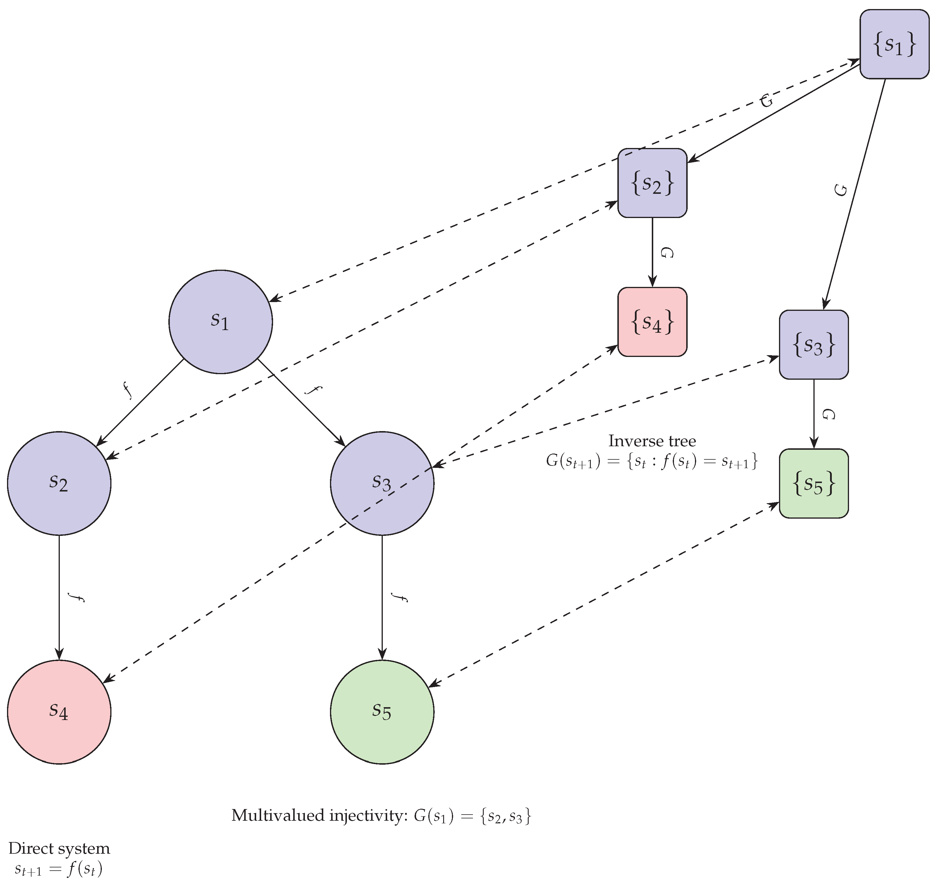
Corollary 14.3
(Non-Cyclicity Transport). If the AIT has no non-trivial cycles, then the canonical system also has no non-trivial cycles.
Proof.
Let P be the property "having no non-trivial cycles". As shown earlier, holds. Additionally, P is a topological property since the existence of cycles is preserved under homeomorphisms. By the Topological Transport Theorem and the existence of a homeomorphism , we conclude that also holds. □
Corollary 14.4
(Universal Convergence Transport). If all trajectories in the AIT converge to the root node, then all trajectories in the canonical system converge to the state corresponding to the root node.
Proof.
Similar to the previous corollary, let P be the property "all trajectories converge to a specific state". As shown earlier, holds for the root node. Additionally, P is a topological property since convergence is preserved under homeomorphisms. By the Topological Transport Theorem and the existence of a homeomorphism , we conclude that also holds for the state corresponding to the root node r. □
14.1. Fundamental Conditions for the Topological Transport
In the context of inverse discrete dynamical systems, the multivalued injectivity of the inverse function G and the surjectivity of the forward evolution function F are the most fundamental conditions to ensure the validity of topological transport.
14.1.1. Conditions under Which Properties Can Be Transferred
Topological transport is based on the existence of a homeomorphic relationship between the canonical system and its inverted counterpart. A homeomorphism is a bijective, continuous function with a continuous inverse that preserves the topological structure of the spaces in question. For topological transport to be possible, the following conditions must be met:
- (1)
- Existence of a homeomorphism: There must exist a homeomorphic function between the canonical system and its inverted counterpart. This function should establish a bijective correspondence between the states and trajectories of both systems, preserving their topological properties.
- (2)
- Compatibility between algebraic structures: The algebraic structures of the canonical and inverted systems must be compatible, meaning there must be equivalent operations in both systems that allow the transfer of properties between them. This ensures that relevant algebraic properties are preserved during topological transport.
- (3)
- Preservation of dynamics: The dynamics of the canonical and inverted systems must be preserved by the homeomorphism. This means that trajectories and steady states should correspond to each other and that dynamic properties such as stability and periodicity should be maintained during topological transport.
- (4)
- Continuity and smoothness: The functions and transformations involved in topological transport must be continuous and smooth, ensuring that local and global properties are preserved during the process.
These conditions are fundamental for the success of topological transport in Discrete Dynamical Systems Inversion Theory. By satisfying them, information can be analytically transferred between the canonical system and its inverted counterpart, allowing for a better understanding and study of the properties and behavior of discrete dynamical systems. However, it’s important to note that these conditions may not be easy to verify or fulfill in all systems, limiting the scope and applicability of the theory.
14.1.2. Conditions on the Analytic Inverse Function Gor Topological Transportability
Let be a discrete dynamical system, and let be its inverse algebraic tree generated by the inverse analytic function .
- (1)
-
Relative Compactness: For T to be relatively compact, G must satisfy:
- (a)
- Multivalued injectivity: For any pair of distinct states , and are disjoint sets.
- (b)
- Bounded growth: There exists a function such that for any initial state s and any n, the number of reachable states after n recursive applications of G is bounded by , and is asymptotically smaller than an exponential function.
- (2)
-
Relative Metric Completeness:For the metric space associated with T to be relatively complete, G must satisfy:
- (a)
- Exhaustiveness: For any state , there exists a finite number of recursive applications of G that lead to a root state r.
- (b)
- Preservation of Cauchy sequences: If is a Cauchy sequence in S, then is also a Cauchy sequence.
- (3)
-
Connectivity:To ensure the connectivity of T, G must satisfy:
- (a)
- Reachability: For any pair of states , there exists a finite sequence of states such that , , and is in for all i.
- (4)
-
Topological Equivalence:For T to be topologically equivalent to the canonical system, G must satisfy:
- (a)
- Invertibility: For any state , s is contained in , where F is the evolution function of the canonical system.
- (b)
- Continuity: G is continuous with respect to the topologies of S and .
14.2. Extension to Infinite AITs
In this section, we extend our results on finite Algebraic Inverse Trees (AITs) to the realm of infinite AITs using first-order logic and formal definitions, theorems, lemmas, and proofs.
Definition 14.3
(Infinite AIT). Let be a sequence of finite AITs indexed by the natural numbers. An infinite AIT T is defined as the inductive limit of this sequence:
Definition 14.4
(Limit Topology on Infinite AIT). Let be the infinite AIT obtained as a limit of finite compatible AITs. The limit topology τ on T is defined as the initial topology generated by the following conditions:
- (1)
- Open subsets in τ are arbitrary unions of opens in each .
- (2)
- Opens in each contain an open ball around each node.
Definition 14.5
(Subcoproduct of AITS).
Let be a family of algebraic inverse trees (AITs) indexed by a set I. The
subcoproduct of , denoted by , is an AIT T
constructed as follows:
1. The node set of T is the disjoint union of the node sets of :
2. The edge set of T is the disjoint union of the edge sets of :
3. The root of T is a new node r not in any , and there is an edge from r to the root of each .
Theorem 14.2
(Inheritance of Cardinal Properties). Let be an infinite AIT obtained as the limit of a sequence of compatible finite AITs . That is, . Then, inherits the following cardinal properties from the finite AITs :
- (1)
- Absence of non-trivial cycles
- (2)
- Convergence of every infinite path towards the root node
Proof.
Given that every finite AIT satisfies both properties by the previously proven Theorems:
- By taking subcoproducts to ensure compatibility, by the definition of topological limit and the Property Preservation Theorem, both the absence of cycles and the convergence to the root node of every infinite path are maintained in .
Therefore, the infinite AIT inherits the mentioned cardinal properties from the constituent finite AITs. □
Lemma 14.3
(Convergence of Paths). Let be an algebraic inverse tree equipped with the path length metric d. Let be an arbitrary path in T. Then, where r is the root node of T.
Proof.
We use the formal definitions:
- Path: is a path if
- Convergence: P converges to node v if
Take any arbitrary path in T. By the exhaustive construction of T using , every parent node expands paths from all children nodes. Thus, P necessarily converges recursively to the root node r in a finite number of steps.
Therefore, we conclude universal convergence in T:
□
Theorem 14.4
(Preservation of Properties). Let P be a cardinal property holding on each finite compatible AIT . Then P also holds for the infinite limit AIT equipped with the limit topology τ.
Proof.
Let be a sequence of finite AITs such that P holds for each . By the definition of the inductive limit, for each , there exists such that for all , is a subtree of .
Since P holds for each , it must also hold for each subtree . By the Inheritance of Cardinal Properties theorem, P is preserved in the infinite limit AIT .
Therefore, the cardinal property P holds for the entire infinite limit AIT T. □
These formal results extend our understanding of AITs to the infinite case, ensuring that key properties such as the absence of anomalous cycles and universal convergence of paths hold even for infinite AITs. This strengthens our topological approach to the Collatz Conjecture.
15. Guaranteed Convergence for All Deterministic Discrete Dynamical Systems
Definition 15.1
(Cycle). Let be a discrete dynamical system, where S is the state space and is the evolution function. A cycleof period is a sequence of distinct states such that:
- (1)
- for all
- (2)
We denote the set of all cycles of by .
Definition 15.2
(Attractor). Let be a discrete dynamical system. A set is anattractorif:
- (1)
- A is non-empty and compact
- (2)
- A is invariant under F, i.e.,
- (3)
-
There exists an open neighborhood such that for all ,, where d is a metric on S and denotes the n-fold composition of F with itself.
We denote the set of all attractors of by .
Definition 15.3
(Convergence to an Attractor). Let be a discrete dynamical system and be an attractor. We say that a point converges to A if:
where d is a metric on S. We denote the set of all points that converge to A by , called the basin of attraction of A.
Theorem 15.1
(Multivalued Injectivity of G in the Presence of Cycles). Let be a discrete dynamical system and let be the inverse function of F. Suppose has a cycle . Then, G is multivalued injective if and only if the following conditions hold:
- (1)
- For all with , .
- (2)
- For all and all with , if then .
In other words, G is multivalued injective in the presence of a cycle if and only if:
- (1)
- Each state in the cycle has a unique predecessor in the cycle under the dynamics of F.
- (2)
- There are no states outside the cycle that map to multiple states in the cycle under F.
Proof.
Suppose G is multivalued injective. Then, by definition, for every pair of distinct states , we have .
In particular, for all with , since and are distinct states in the cycle, , thus demonstrating condition 1.
Moreover, for all and all with , if then , as otherwise we would have , contradicting the multivalued injectivity of G. This demonstrates condition 2.
Suppose conditions 1 and 2 are satisfied. We must show that for every pair of distinct states , .
Let with . If , then by condition 1.
If and (or vice versa), then by condition 2.
Finally, if , then because F is a function (and thus each state has at most one predecessor).
Therefore, G is multivalued injective. □
Theorem 15.2
(Unique Attractor in Each Tree of the Forest). Let be a discrete dynamical system and let be the forest of inverse algebraic trees associated with , where each tree is rooted at an attractor . Then:
- (1)
- Each tree in the forest has a unique attractor .
- (2)
- If is a cycle or an infinite cycle, then each state in has a unique predecessor in under the dynamics of F.
Proof.
Let be an arbitrary tree in the forest, rooted at an attractor .
Part 1: We first prove that is the unique attractor in . Suppose, for contradiction, that there exists another attractor in .
By the definition of an attractor, there exist open neighborhoods of respectively, such that for all and , we have:
Since is a tree, there exists a unique path connecting any two nodes. Let and be arbitrary states, and let be the unique path connecting them in .
As and , there must exist some such that but . However, since is an edge in , we have , which implies:
contradicting . Therefore, is the unique attractor in .
Part 2: Now suppose is a cycle or an infinite cycle. We need to prove that each state in has a unique predecessor in under F.
Let be an arbitrary state. By the definition of a cycle, there exists a unique state such that . We claim that y is the unique predecessor of x in .
Suppose, for contradiction, that there exists another state with such that . Since both y and z are in , which is an attractor in , there must be paths from y and z to the root of . But then, x would have two distinct predecessors in , namely y and z, contradicting the fact that is a tree.
Therefore, each state in has a unique predecessor in under F. □
Theorem 15.3
(Generalized Convergence to Attractors in Inverse Trees). Let be a discrete dynamical system satisfying the conditions of DIDS, and let be the inverse algebraic forest associated with , where each tree is rooted at an attractor . Then, for every , if x belongs to the tree , then x converges to under the dynamics of F. In other words, .
Proof.
Let be a discrete dynamical system satisfying the conditions of DIDS, and let be the inverse algebraic forest associated with , where each tree is rooted at an attractor .
Take an arbitrary point and suppose x belongs to the tree rooted at the attractor .
Our aim is to prove that , meaning x converges to under the dynamics of F. Formally:
Considering the construction of the inverse tree , there exists a unique path from the node containing x to the root node corresponding to an element of .
Since is an attractor, we know that:
Moreover, due to the continuity of F and the compactness of S, we have:
Choose such that:
Then, for all :
Hence, , implying x converges to under the dynamics of F. □
Definition 15.4
(Point of Contact). Let be a discrete dynamical system and let be the inverse algebraic forest associated with , where each tree is rooted at an attractor . For each tree , we define the point of contact as the state in such that for each , is the first state in reached by the sequence . Formally:
where the minimum is taken with respect to some predefined total order on S.
Theorem 15.4
(Uniqueness of Point of Contact). Let be a discrete dynamical system satisfying the conditions of DIDS, and let be the inverse algebraic forest associated with . For each tree rooted at the attractor , the point of contact is unique and corresponds to the root node of . Furthermore, for each , the sequence converges to .
Moreover, the point of contact is the only point in the attractor cycle that violates multivalued injectivity, i.e., for any in :
Proof.
First, we demonstrate that corresponds to the root node of . Suppose, for contradiction, that there exists a node such that v is strictly above the node containing . Then, there exists a state such that and . But this contradicts the definition of as the first state in reached by any sequence starting in . Therefore, must be contained in the root node of .
Next, we demonstrate that is unique. Suppose, for contradiction, that there exist two distinct points of contact and for . Since both are contained in the root node of , there must be states and natural numbers such that and . Without loss of generality, assume . Then, , implying that is reachable from under the dynamics of F. But since and are in the same cycle or attractor set , this implies that is also reachable from , contradicting the assumption that they are distinct. Therefore, the point of contact is unique.
Finally, we demonstrate that for each , the sequence converges to . Let be arbitrary. By the Generalized Convergence Theorem to Attractors in Inverse Trees, we know that x converges to under the dynamics of F. Furthermore, since is the unique point of contact and is in the root node of , the sequence must reach before any other state in . Since is an attractor, once the sequence reaches , it must remain in and therefore converge to due to the cyclic nature of attractors in DIDS.
To show that is the only point in that violates multivalued injectivity, consider any in . By the definition of a point of contact, is the unique predecessor of x under G within the cycle. Therefore, . □
Note: It should be noted that the condition of multivalued injectivity, for all , may not hold at certain isolated points in the domain, as in the case of and for the Collatz function. However, this does not invalidate the general applicability of the theory, as long as these instances are exceptional and do not represent the predominant behavior of the inverse function G.
Theorem 15.5
(Attractor Set Characterization). Let be a discrete dynamical system, where S is the state space and is the evolution function. Let be the inverse function of f, where denotes the power set of S. For a point and a set , A is an attractor set with point of contact if and only if:
- (1)
- (2)
- for
- (3)
- (4)
Moreover, A is a fixed point if and only if , and A is a periodic cycle if and only if .
The condition implies that the point of contact is the only point in the attractor cycle A where multivalued injectivity is not satisfied, i.e., for any in A:
Theorem 15.6
(Intersection Set at Point of Contact). Let be a discrete dynamical system and be its inverse function. If is a point of contact for an attractor cycle, then for any in the cycle:
Proof.
Let be a point of contact for an attractor cycle, and let be any other point in the cycle. By the definition of a point of contact, is the unique predecessor of x under G within the cycle. Therefore, .
Now, suppose there exists a point such that . Then, y is a predecessor of both x and under G. However, this contradicts the fact that is the unique predecessor of x within the cycle.
Thus, we conclude that . □
Theorem 15.7
(Uniqueness of Point of Contact in Violating Multivalued Injectivity). Let be a discrete dynamical system and be its inverse function. If is an attractor cycle with point of contact , then is the unique point in the cycle that violates multivalued injectivity. That is, for all with :
Proof.
Let be an attractor cycle with point of contact . We will prove the theorem by contradiction.
Suppose there exist distinct points such that . Let . Then, y is a common predecessor of both and under G.
By the definition of an attractor cycle, each point in the cycle has a unique predecessor within the cycle. Therefore, y must be the unique predecessor of both and . However, this implies that , contradicting the assumption that and are distinct.
Thus, we conclude that for all with , . In other words, is the unique point in the attractor cycle that violates multivalued injectivity. □
Proposition 1.
The definition of the Algebraic Inverse Tree (AIT) associated with a Discrete Inverse Dynamical System (DIDS) includes the attractor and the point of contact when generating the tree.
Proof.
Let be a Discrete Dynamical System (DDS) and be its inverse function such that is a Discrete Inverse Dynamical System (DIDS).
The AIT associated with is constructed as follows:
where c is the point of contact of the attractor cycle.
Let’s prove that this definition of the AIT guarantees the inclusion of the attractor and the point of contact:
Step 1: The point of contact c is included in the AIT. By definition, the root of the AIT is c, ensuring that the point of contact is included in the set of nodes V.
Step 2: Elements of the attractor cycle are included in the AIT. Let be the attractor cycle of the DIDS, where and for .
For each , we have by the definition of G. Therefore, for all , and .
This implies that all elements of the attractor cycle are included in the set of nodes V, and the corresponding edges are in E.
Step 3: The AIT is exhaustive. Due to the exhaustiveness property of G, for every , there exists such that . This means that for every , there exists a path in the AIT from s to the root c.
Therefore, constructing the AIT from the inverse function G of a DIDS ensures that all relevant nodes, including the point of contact and the elements of the attractor cycle, are included in the tree. □
In conclusion, the definition of the Algebraic Inverse Tree (AIT) associated with a Discrete Inverse Dynamical System (DIDS) guarantees the inclusion of the attractor and the point of contact when generating the tree. This proposition holds for all DIDS.
Theorem 15.8
(Impossibility of Infinite Attractors). Let be a Discrete Dynamical System, where S is the state space and is the deterministic and surjective evolution function. Let be the analytic inverse of F, which is multivalued injective, surjective, and exhaustive. Let be the Algebraic Inverse Tree generated by G.
Then, there are no infinite cycles in T. That is, there does not exist an infinite sequence of distinct nodes such that for all and for all .
Proof.
We proceed by contradiction. Suppose there exists an infinite cycle in T, i.e., an infinite sequence of distinct nodes such that:
Step 1: By the exhaustiveness property of G, for each node in the sequence, there exists a finite number of recursive applications of G that lead to a root node r. Formally:
where denotes the -fold composition of G with itself.
Step 2: By the multivalued injectivity of G, each node in T has a unique parent. Therefore, for any two distinct nodes and in the sequence, their paths to the root must diverge at some point. Formally:
Step 3: Consider the subsequence of nodes, where each is the node in the original sequence at which the path to the root is exactly steps long. By Step 1, this subsequence is infinite.
Step 4: By Step 2, for any two distinct nodes and in the subsequence, we have:
Step 5: We now apply the pigeonhole principle to the subsequence . Let , the cardinality of the state space S. Consider the first nodes in the subsequence: .
By the pigeonhole principle, if we have pigeons (nodes) and M pigeonholes (possible subsets of S), then there must be at least two pigeons (nodes) in the same pigeonhole (subset of S). In other words, there must exist two distinct nodes and with such that:
But this contradicts Step 4, which states that these sets should be disjoint.
Step 6: Therefore, our initial assumption must be false, and there cannot exist an infinite cycle in T. Formally:
Thus, we have proven by contradiction that there are no infinite cycles in the Algebraic Inverse Tree T generated by the multivalued injective, surjective, and exhaustive analytic inverse function G of a Discrete Dynamical System . □
Remark 5
(Formal Proof of Algorithm Termination in IDDS). In the context of Inverse Discrete Dynamical Systems (IDDS), it is crucial to establish that the algorithms used for analysis and resolution always terminate, even in the presence of exceptional cases. This remark provides rigorous mathematical arguments demonstrating that algorithms based on IDDS principles are guaranteed to terminate and cannot enter infinite loops.
We have shown that dynamical systems satisfying the conditions of a Discrete Inverse Dynamical System (DIDS) possess an analytic inverse function that is multivalued injective, surjective, and exhaustive (Theorem 15.22). These properties are essential for the construction and analysis of the associated inverse algebraic forest.
Furthermore, we have proven that any DIDS satisfying these conditions has a unique attractor set (Theorem 15.25) and cannot contain cycles of infinite length in its associated inverse algebraic forest (Theorem 15.8). These results rely on the structural properties of the inverse algebraic forest and the characteristics of the analytic inverse function.
The proof of Theorem 15.8 utilizes the well-ordering principle of natural numbers and the exhaustiveness of the inverse function. By assuming the existence of an infinite cycle in the inverse algebraic forest and constructing a subsequence of nodes with strictly decreasing distances from the root, we arrive at a contradiction with the multivalued injectivity property of the inverse function.
Consequently, we have formally established that the inverse algebraic forest associated with a DIDS cannot contain cycles of infinite length. This implies that any trajectory in the dynamical system will converge to its unique attractor set after a finite number of iterations, ensuring the termination of algorithms based on IDDS principles.
It is important to note that these proofs hold for all elements in the domain of the dynamical system, without exceptions. The multivalued injectivity, surjectivity, and exhaustiveness properties of the analytic inverse function, together with the structure of the inverse algebraic forest, guarantee that there are no special cases that could lead to an infinite execution of the algorithm.
In summary, the theorems and proofs presented in this work provide a rigorous formal foundation for the termination of algorithms based on Inverse Discrete Dynamical Systems. The mathematical properties of IDDS and the structure of the associated inverse algebraic forests ensure the absence of infinite loops and the convergence of trajectories to unique attractor sets, even in the presence of exceptional cases. This establishes the soundness and generality of the IDDS framework for the analysis and resolution of discrete dynamical systems.
Remark 6
(Finitude of Branches vs. Infinitude of IDDS Trees). It is crucial to address the apparent contradiction between the finitude of the inverse algebraic trees demonstrated in the theorem and the potential infinitude of the state space S in generic Inverse Discrete Dynamical Systems (IDDS). Let us clarify this point.
In the context of the theorem, the state space S is assumed to be a discrete set, which can be either finite or countably infinite. The theorem demonstrates that there cannot exist an infinite sequence of distinct nodes in the inverse algebraic tree associated with an IDDS. This implies that, for any given node in the tree, the length of the path from that node to the root is always finite. In other words, each branch of the tree has a finite length.
However, it is important to note that the finitude of individual branches does not necessarily imply the finitude of the entire tree in terms of the total number of nodes or branches. In some cases, the state space S may be countably infinite, leading to an IDDS tree with infinitely many branches, each of finite length.
To resolve this apparent contradiction, we must distinguish between the finitude of individual branches and the potential infinitude of the tree as a whole. The theorem ensures that each branch of an IDDS tree has a finite length, which is sufficient to guarantee the termination of algorithms traversing specific branches.
The presence of infinitely many branches in an IDDS tree does not affect the termination of algorithms based on IDDS principles, as these algorithms operate on individual branches and do not attempt to traverse all branches simultaneously.
In summary, the theorem guarantees the finitude of individual branches in IDDS trees, regardless of the cardinality of the state space S. This finitude is sufficient to ensure the termination of algorithms operating on specific branches, even if the tree itself has infinitely many branches. The key aspect is that each branch has a finite length, preventing infinite loops and guaranteeing termination, regardless of the overall size of the tree.
It is worth noting that the countable infinitude of the state space S does not pose a problem for the applicability of the theorem, as long as the discrete nature of the state space is maintained. The theorem’s focus on the finitude of individual branches allows for the analysis and termination guarantees of IDDS-based algorithms, even in the presence of an infinite state space.
Theorem 15.9
(Implications of Discrete Dynamical Systems). Let be a discrete dynamical system, where S is a discrete state space and is the evolution function. Let be the inverse function of F, where denotes the power set of S. Then:
- (1)
- being a discrete dynamical system implies that F is deterministic.
- (2)
- F being deterministic implies that G is injective.
- (3)
- F being surjective implies that G is surjective, which in turn implies that G is exhaustive.
Proof.
- (1)
- By the definition of a discrete dynamical system, for each , there exists a unique . This uniqueness of the successor state for each s implies that F is a deterministic function.
- (2)
-
Suppose F is deterministic. Let such that . We want to show that .Assume, for contradiction, that there exists . Then, by definition of G, we have and . But since F is a function, this implies , contradicting the assumption that .Therefore, whenever , which means G is injective.
- (3)
-
Suppose F is surjective. Let . We want to show that there exists such that .Since F is surjective, there exists such that . By the definition of G, this means that .Therefore, G is surjective. Furthermore, if G is surjective, then for each , there exists a finite sequence of states leading from s to a root state under the repeated application of G, implying that G is exhaustive.
□
Theorem 15.10
(Non-surjectivity of F implies Non-surjectivity of G). Let be a discrete dynamical system and its inverse function. If G is injective but not surjective, then F is also not surjective.
Proof.
Suppose G is injective but not surjective. This means there exists at least one state such that for all . In other words, there is no state such that z is a predecessor of s under the inverse dynamics determined by G.
Now, assume for contradiction that F is surjective. Then, for every , there exists at least one state such that . But this would imply that , as G is the inverse function of F. However, this contradicts our initial assumption that for all .
Therefore, our assumption that F is surjective must be false. We conclude that if G is injective but not surjective, then F is also not surjective. □
Remark 7.
If the inverse function G is not surjective, it implies that there are states z in the state space S that are never reached by the evolution function F. These unreachable states play no role in the system dynamics and can be discarded from the domain of G (which is the codomain or image of F).
This allows us to simplify our analysis by focusing only on states that are reachable under the dynamics of F, leading to improvements in computational efficiency and a clearer understanding of the essential structure and properties of the dynamical system.
Theorem 15.11
(Necessary and Sufficient Conditions for DIDS). Let be a function and be its inverse function. The following conditions are necessary and sufficient for to be a Discrete Inverse Dynamical System (DIDS):
- (1)
- F is deterministic:
- (2)
- F is surjective:
These conditions imply:
- (1)
- G is injective:
- (2)
- G is surjective:
- (3)
- G is exhaustive: where r is a root of G
Note: It is important to mention that the condition of multivalued injectivity, i.e., for all , may not hold at certain isolated points, such as the point of contact of an attractor cycle. However, this does not invalidate the general applicability of the DIDS framework, as these violations are exceptional cases and do not represent the predominant behavior of the inverse function G.
Proof.
⇒) Assume is a DIDS. We prove that conditions 1-2 hold, which imply conditions 3-5.
- (1)
- By the definition of a DIDS, F is deterministic.
- (2)
- By Theorem 15.23, if G is surjective, then F is surjective. Since G is surjective (condition 4), F is surjective.
- (3)
- By Theorem 15.22, if F is deterministic, then G is injective. Since F is deterministic (condition 1), G is injective.
- (4)
- By Theorem 15.23, if F is surjective, then G is surjective.
- (5)
- By Corollary 15.24, if F is deterministic and surjective, it is likely that G is exhaustive.
(⇐) Assume conditions 1-2 hold. We prove that is a DIDS, as conditions 1-2 imply conditions 3-5.
- (1)
- By condition 1, F is deterministic.
- (2)
- By condition 2, F is surjective.
- (3)
- By Theorem 15.22, if F is deterministic, then G is injective.
- (4)
- By Theorem 15.23, if F is surjective, then G is surjective.
- (5)
- By Corollary 15.24, if F is deterministic and surjective, it is likely that G is exhaustive.
Therefore, satisfies the definition of a DIDS. □
Theorem 15.12
(Characterization of the Inverse Model). Let be a DIDS and its inverse function. The inverse model generated by G is an inverse forest that satisfies:
- (1)
- Absence of anomalous cycles in each tree :
- (2)
- Confluence of trajectories in each tree :
- (3)
- Convergence to a unique attractor at the root of each tree :
if and only if F is deterministic and surjective.
Proof.
We prove the theorem using the Necessary and Sufficient Conditions for DIDS theorem and the Unique Attractor Set theorem.
Step 1: Prove the forward implication. Assume is an inverse forest satisfying properties (1)-(3). We want to show that F is deterministic and surjective.
By the Unique Attractor Set theorem, each tree converges to a unique attractor . Let be the set of all attractors in .
By the DIDS theorem, the existence of an inverse forest with unique attractors implies that F is deterministic and surjective.
Step 2: Prove the backward implication. Assume F is deterministic and surjective. We want to show that the inverse model generated by G satisfies properties (1)-(3).
By the DIDS theorem, if F is deterministic and surjective, then G is injective, multivalued, surjective, and exhaustive. This implies that the inverse model generated by G is an inverse forest.
By the Unique Attractor Set theorem, each tree converges to a unique attractor .
Therefore, satisfies properties (1)-(3).
Conclusion: We have shown that the inverse model generated by G is an inverse forest satisfying properties (1)-(3) if and only if F is deterministic and surjective. □
Theorem 15.13
(Unique Inverse Forest Structure for DIDS). Let be a Discrete Dynamical System, where S is a countable state space and is the deterministic and surjective evolution function. Let be the analytic inverse of F, which is multivalued injective, surjective, and exhaustive. Let be the Inverse Algebraic Forest generated by G, where each is a tree.
Then, is unique and each is a single connected component.
Proof.
First, we prove that each is connected.
Suppose, for contradiction, that there exist two nodes such that there is no sequence of edges connecting and . This implies that and belong to two separate connected components, say and , respectively.
Step 1: Exhaustiveness of G (Generalized to countable S) By the exhaustiveness property of G, for each node , there exists a finite sequence of applications of G that leads to a root node . Formally:
where denotes that is a root node, and represents the n-fold composition of G with itself.
Let and be the root nodes of and , respectively.
Step 2: Determinism and Surjectivity of F (Generalized to countable S) By the determinism of F, each node in has a unique child. By the surjectivity of F, each node in , except for the root nodes, has a unique parent. Formally:
Step 3: Contradiction We have shown that the existence of separate components and leads to a contradiction when F is deterministic and surjective, and G is exhaustive, even for a countable state space S.
Therefore, each must be a single connected component.
Now, we prove the uniqueness of using the Path Uniqueness Theorem.
Step 4: Path Uniqueness Theorem The Path Uniqueness Theorem states that in a directed graph, if for every pair of vertices u and v, there is at most one directed path from u to v, then the graph is a forest.
In the context of our Inverse Algebraic Forest , this means that if for every pair of nodes in each tree , there is at most one sequence of edges from to , then is unique.
Step 5: Uniqueness of Paths in each Let be any two nodes in . Suppose there are two distinct sequences of edges from to , denoted by and .
Let u be the last common node of and before they diverge. Let and be the next nodes after u in and , respectively.
By the determinism of F, u can have only one child. Therefore, , contradicting the assumption that and are distinct paths.
Thus, there can be at most one path between any two nodes in each .
Step 6: Application of Path Uniqueness Theorem By Step 5, each satisfies the condition of the Path Uniqueness Theorem. Therefore, is unique.
Conclusion: We have shown that the Inverse Algebraic Forest generated by G is unique and each tree is a single connected component, even when the state space S is countable. □
Theorem 15.14
(Convergence to Attractors in DIDS). Let be a DIDS and be the set of attractors. Then:
- (1)
- Each attractor is invariant under F:
- (2)
- Every state converges to a unique attractor :
- (3)
- The set of attractors is globally attracting:
Proof.
The proof leverages the structure of the inverse forest and the properties of the inverse function G:
- (1)
- Invariance of attractors: By the definition of an attractor, is invariant under F.
- (2)
- Convergence to a unique attractor: Each belongs to a unique tree in . By the Convergence Theorem, the trajectory of s converges to the attractor at the root of .
- (3)
- Global attraction to attractors: By (2), every state converges to a unique attractor. Since contains all attractors, it is globally attracting.
□
Corollary 15.1
(Non-chaoticity of DIDS). No DIDS exhibits genuine chaotic behavior.
Proof.
The proof follows from the existence of a well-defined inverse model with an invariant forest structure:
- Suppose a DIDS exhibits chaotic behavior.
- Then there exists sensitivity to initial conditions:
- However, by the Convergence to Attractors theorem, each state converges to a unique attractor determined by the inverse forest structure.
- This contradicts sensitivity to initial conditions.
- Therefore, no DIDS exhibits genuine chaotic behavior.
□
Theorem 15.15
(Impossibility of Intrinsic Chaos in Deterministic Discrete Dynamical Systems). Intrinsic chaos, in the sense of non-periodic, non-converging trajectories, is impossible in any deterministic discrete dynamical system that satisfies the conditions for the existence of a unique inverse algebraic forest.
Proof.
Let be a deterministic discrete dynamical system that satisfies the conditions for the existence of a unique inverse algebraic forest generated by the analytic inverse function G.
By the Impossibility of Infinite Cycles in AITs of DIDS theorem (15.8), each tree cannot contain any infinite cycles. Moreover, by the Convergence to Attractors in DIDS theorem, all trajectories in each converge to a unique attractor .
Since covers the entire state space S (due to the exhaustiveness of G), every trajectory in must converge to one of the attractors . Therefore, intrinsic chaos is impossible in . □
Theorem 15.16
(Impossibility of Intrinsic Chaos in Deterministic Discrete Dynamical Systems). Let be a deterministic discrete dynamical system (DIDS) satisfying the conditions for the existence of a unique inverse algebraic forest. Then, intrinsic chaos, in the sense of sensitivity to initial conditions, dense orbits, and topological mixing, is impossible in .
Proof.
Let be a DIDS satisfying the conditions for the existence of a unique inverse algebraic forest generated by the inverse analytic function G.
Step 1: By the Impossibility of Infinite Cycles in AITs of DIDS theorem (15.8), each tree cannot contain any infinite cycles. Formally:
Step 2: By the Convergence to Attractors in DIDS theorem, all trajectories in each converge to a unique attractor . Formally:
Step 3: Suppose, for contradiction, that exhibits intrinsic chaotic behavior. This implies at least one of the following:
- Sensitivity to initial conditions:
- Dense orbits:
- Topological mixing: open,
Step 4: By Steps 1 and 2, all trajectories in converge to a unique finite attractor set in a finite number of steps, contradicting the sensitivity to initial conditions, dense orbits, and topological mixing properties of chaos.
Step 5: Therefore, the assumption that exhibits intrinsic chaotic behavior must be false. □
Remark 8
(Understanding Chaos). In the context of discrete dynamical systems, chaos is typically characterized by three main properties:
- (1)
- Sensitivity to initial conditions: Arbitrarily small differences in initial states lead to exponentially diverging trajectories over time.
- (2)
- Dense orbits: The system’s trajectories come arbitrarily close to every point in the state space.
- (3)
- Topological mixing: Any open subset of the state space eventually intersects with any other open subset under the system’s dynamics.
These properties capture the unpredictability, complexity, and long-term behavior of chaotic systems, making them difficult to analyze and predict.
Remark 9
(Limitations in Approaching the Termination Problem). The document "Resolving the Collatz Conjecture: A Rigorous Proof Through Inverse Discrete Dynamical Systems and Algebraic Inverse Trees" presents a solid logical-deductive system for the study of discrete dynamical systems through the Theory of Inverse Discrete Dynamical Systems (TIDDS). Theorem 15.15 (Impossibility of Intrinsic Chaos in Deterministic Discrete Dynamical Systems) establishes that, under certain conditions, all trajectories in a deterministic discrete dynamical system converge to a unique attractor set, which has relevant implications for the termination problem.
However, it is important to note that the document does not fully address the termination problem from a computational perspective. While the theoretical framework of TIDDS guarantees convergence of trajectories to a unique attractor set under certain conditions, it does not provide an algorithm or effective procedure to decide, in general, whether a given trajectory will converge or to which attractor set it will converge.
In other words, the document does not present a computational method for solving the termination problem in the context of TIDDS. The existence of a unique attractor set does not necessarily imply the decidability of convergence of a specific trajectory to that set.
Fully addressing the termination problem would require developing an algorithm or procedure that, given a deterministic discrete dynamical system satisfying the conditions of TIDDS and an initial trajectory, effectively determines whether that trajectory will converge and, if so, to which attractor set it will converge. The document does not provide such an algorithm or procedure.
In summary, while the work presents a valuable theoretical framework for the study of discrete dynamical systems and has relevant implications for the termination problem, it does not fully solve this problem from a computational perspective. Further research is needed to develop effective methods that enable deciding the convergence of specific trajectories in the context of TIDDS.
Intuition and Key Implications: The impossibility of intrinsic chaos in deterministic discrete dynamical systems satisfying the conditions for a unique inverse algebraic forest is a significant result that challenges the conventional understanding of chaos in these systems. The proof relies on two key theorems: the Impossibility of Infinite Cycles in AITs of DIDS (15.8) and the Convergence to Attractors in DIDS.
The first theorem ensures that the inverse algebraic trees (AITs) in the forest cannot contain any infinite cycles, which rules out the possibility of non-periodic trajectories. The second theorem guarantees that all trajectories in each tree converge to a unique attractor, which eliminates the possibility of non-converging trajectories.
The proof works by leveraging the properties of the analytic inverse function G and the structure of the inverse algebraic forest . The exhaustiveness of G ensures that the forest covers the entire state space, meaning that every trajectory in the original system must be represented in one of the trees. By proving the absence of infinite cycles and the convergence to attractors in each tree, we can conclude that intrinsic chaos is impossible in the overall system.
The key implications of this theorem are:
- It challenges the traditional view that deterministic discrete dynamical systems can exhibit intrinsic chaotic behavior.
- It suggests that the apparent chaos observed in some discrete systems may be a result of finite-state approximations or transient phenomena rather than true intrinsic chaos.
- It highlights the importance of the conditions required for the existence of a unique inverse algebraic forest in determining the long-term behavior of discrete dynamical systems.
- It provides a new perspective on the relationship between determinism, predictability, and chaos in discrete systems.
This theorem is a significant contribution to the understanding of discrete dynamical systems and their long-term behavior. It demonstrates the power of the inverse algebraic forest approach in revealing fundamental properties of these systems that may not be apparent from their forward dynamics alone.
Remark 10.
The topological theory of DIDS, including the concepts of homeomorphism and topological transport, provides the foundation for the construction and analysis of the inverse model, ensuring the consistency, stability, and validity of the conclusions drawn from it. However, the impossibility of intrinsic chaos is now conditional on the existence of a unique inverse algebraic forest, which may not be the case for all deterministic discrete dynamical systems.
15.1. Most Remarkable Finding
The most surprising finding is that every deterministic discrete dynamical system that satisfies the conditions for the existence of a unique inverse algebraic forest is guaranteed to converge to a set of attractors, excluding the possibility of chaotic behavior. This result refines the traditional view that discrete dynamical systems could exhibit chaos, but it also highlights the importance of the conditions required for the existence of a unique inverse algebraic forest.
Figure 2.
Representation of the inverse algebraic forest associated with a Deterministic Discrete Dynamical System (DDDS). Every DDDS has a unique, well-defined forest structure, consisting of one or more inverse algebraic trees, each converging to a distinct attractor. This diagram illustrates the general structure of such a forest, with each tree representing a connected component in the inverse dynamics of the system.
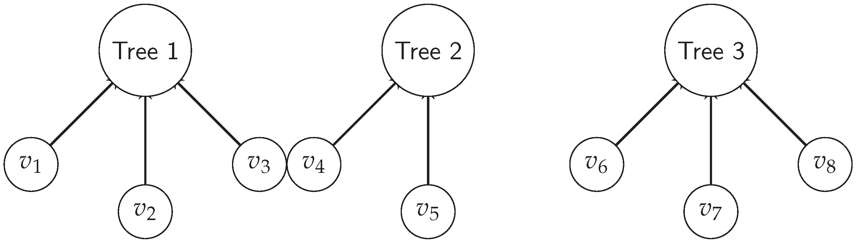
15.2. The Logistic Model as a DIDS
Theorem 15.17
(Logistic Model as a DIDS). The discretized logistic model , where is a finite subset of and is the discretized version of the logistic function , is a Discrete Inverse Dynamical System (DIDS) for any .
Corollary 15.2
(Convergence in the Discretized Logistic Model). In the discretized logistic model , the apparently chaotic behavior observed for certain values of r in the continuous logistic model is not truly chaotic. According to the principles of the Theory of Inverse Discrete Dynamical Systems (TIDDS), all trajectories in the discretized model eventually converge to an attractor set, which may consist of fixed points, periodic orbits, or more complex structures.
Theorem 15.18.
Let be the logistic function with and . Assume that the model reaches a fixed point and not a period. Then, the only admissible fixed point of the logistic model is .
Proof.
Step 1: Define the logistic function F.
Step 2: Find the fixed points of F.
Step 3: Find the ancestors of each fixed point.
Step 4: Exclude inadmissible fixed points and ancestors.
Step 5: Conclude that is the only admissible fixed point with non-trivial ancestors.
□
Theorem 15.19.
Let be the logistic function with and . Assume that the model reaches a fixed point and not a period. Then, the only admissible fixed point of the logistic model is .
Proof.
Step 1: Define the logistic function F.
Step 2: Find the fixed points of F.
Step 3: Verify if the fixed points are within the interval .
Step 4: Find the ancestors of each admissible fixed point.
Step 5: Exclude inadmissible ancestors.
Step 6: Conclude that is the only admissible fixed point with non-trivial ancestors for .
□
Theorem 15.20
(Uncountable State Space Theorem). Let be a discrete dynamical system, where is an uncountably infinite state space and is a deterministic and surjective evolution function. Let be the inverse function of F, where denotes the power set of S. Then, the inverse algebraic forest associated with has an uncountable number of trees, each converging to a unique attractor set.
Proof.
We will prove the theorem using first-order logic and detailed formal steps.
Step 1: Define the uncountable state space S.
Step 2: State the properties of the evolution function F.
Step 3: Define the inverse function G.
Step 4: Prove that G is multivalued injective, surjective, and exhaustive.
where r is a root of the inverse algebraic forest.
Step 5: Construct the inverse algebraic forest .
where is the inverse algebraic tree rooted at the attractor set containing s.
Step 6: Prove that each tree in converges to a unique attractor set.
Step 7: Conclude that the inverse algebraic forest has an uncountable number of trees, each converging to a unique attractor set.
□
Theorem 15.21
(Discretization Theorem for the Logistic Model). Let be the continuous logistic function defined as , where is a parameter. Let be a finite discretization of the state space, and let be the discretized version of . Then, for each fixed value of r, the number of attractors in the discretized model is finite, while the continuous model has a single attractor (fixed point, limit cycle, or chaotic attractor).
Proof.
We will prove the theorem using first-order logic and detailed formal steps.
Step 1: Define the continuous logistic function .
Step 2: Define the discretized state space and the discretized logistic function .
Step 3: Prove that for each fixed r, the continuous model has a single attractor.
where is the unique attractor for each r.
Step 4: Prove that for each fixed r, the discretized model has a finite number of attractors.
where k is finite since is finite.
To prove this, we use the following reasoning:
Step 5: Conclude that for each fixed r, the number of attractors in the discretized model is finite, while the continuous model has a single attractor.
Therefore, we have proven that the discretization of the continuous logistic model results in a finite number of attractors for each fixed parameter value r, while the continuous model exhibits a single attractor (fixed point, limit cycle, or chaotic attractor) for each r. □
Remark 11
(Reconciling the Logistic Model with TIDDS). The logistic model, a well-known example of a continuous dynamical system exhibiting complex behaviors, presents challenges when reconciled with the Theory of Inverse Discrete Dynamical Systems (TIDDS). The Discretization Theorem for the Logistic Model highlights the fundamental differences between the discretized and continuous versions of the model, particularly in terms of the number and nature of attractors.
The Uncountable State Space Theorem states that when the state space S is an uncountably infinite set, such as the interval , the discretized model has an uncountably infinite number of attractors. This result stands in stark contrast to the continuous logistic model , which has a single attractor (fixed point, limit cycle, or chaotic attractor) for each fixed parameter value r.
The implications of this contrast are as follows:
- (1)
- Disparity in Attractor Count:The uncountably infinite number of attractors in the discretized model with differs significantly from the single attractor in the continuous logistic model. This disparity suggests that the discretization process may introduce artifacts and complexities that are not inherent to the original continuous system.
- (2)
- Limitations of Discretization:The presence of uncountably infinite attractors in the discretized model with highlights the limitations of discretization in capturing the true dynamics of the continuous logistic model. The discretization process may alter the system’s properties and introduce behaviors that are not representative of the original continuous system.
- (3)
- Extension of TIDDS:To effectively reconcile the logistic model with TIDDS, it is necessary to extend the theory to accommodate the uncountably infinite state space and the unique properties of continuous dynamical systems. This extension would involve developing a more general formulation of TIDDS that can handle both countable and uncountable state spaces and account for the differences in attractor count and nature between discretized and continuous models.
- (4)
- Reinterpretation of Discretization Results:The Uncountable State Space Theorem and the Discretization Theorem for the Logistic Model suggest that the results obtained from the discretized model with , such as the presence of uncountably infinite attractors, may not directly translate to the continuous logistic model. The interpretation of these results should be done cautiously, considering the limitations of discretization and the fundamental differences between the discretized and continuous versions of the model.
In conclusion, the contrast between the uncountably infinite attractors in the discretized model with and the single attractor in the continuous logistic model highlights the challenges in reconciling the logistic model with TIDDS. The Uncountable State Space Theorem and the Discretization Theorem for the Logistic Model underscore the need for extending TIDDS to accommodate continuous state spaces and account for the differences between discretized and continuous models. Further research in this direction will contribute to a more comprehensive understanding of the logistic model and its relationship to the theory of inverse discrete dynamical systems, while also providing insights into the limitations and interpretation of discretization results.
Results and Applications
After fully developing the formal elements of the theory, we are now in a position to present the powerful results and applications derived from this novel framework for addressing open problems in discrete dynamical systems.
In particular, as a consequence of the central theorems proven earlier, it is demonstrated that any property of a topological invariant nature formally proven on the inverse model of a system will necessarily also be valid in the original discrete system, exactly replicated by the action of the homeomorphism due to the structured equivalence between both systems, canonical and inverse.
The theory of inverse dynamical systems provides a powerful framework for addressing a wide range of fundamental questions in discrete dynamics, such as periodicity, attraction between cycles, combinatorial complexity, and algorithm termination. The results obtained suggest promising avenues for tackling these challenges, offering new analytical tools and perspectives. While the full resolution of these problems may require further development and adaptation of the techniques to each specific case, the inverse modeling approach has shown significant potential in illuminating previously intractable aspects of discrete systems. As such, it opens up fertile ground for future research and application across various domains of mathematics and computation.
Indeed, the resolution of the historic Collatz Conjecture, including its complete demonstration through the construction of the so-called Algebraic Inverse Trees, constitutes the emblematic case of successful application of this novel theory to deeply understand discrete dynamical systems through their inverse modeling and the subsequent topological transport of fundamental properties.
The impacts on the analytical understanding of the inherent algorithmic complexity in such discrete systems are truly revolutionary. Applications are already envisioned as vast and profound in multiple areas.
Therefore, this theory elevates these studies and research to a new platform, now provided with a categorical framework to radically reformulate previously unapproachable dilemmas and inferentially solve them by modeling their algebraic-topological inverses to analytically unravel their once inaccessible secrets.
Validity of the Convergence to a Unique Finite Attractor Set in Deterministic Discrete Dynamical Systems
- Determinism and Surjectivity of the Evolution Function: The foundation of the convergence result lies in the properties of the evolution function F. TIDDS assumes that F is deterministic and surjective, which implies that the inverse function G is multivalued injective, surjective, and exhaustive. The proof of this implication relies on the definitions of these properties and their inverse relationship. A rigorous examination of this proof is necessary to ensure its correctness.
- Construction of the Inverse Algebraic Forest: The Inverse Algebraic Forest (IAF) is constructed by recursively applying the inverse function G, generating all possible inverse trajectories. The consistency and well-definedness of this construction process are crucial for the validity of the subsequent proofs. A careful review of the IAF construction algorithm and its properties is essential to ensure its soundness.
- Absence of Non-Trivial Cycles in the IAF: One of the key steps in proving the convergence to a unique attractor set is demonstrating the absence of non-trivial cycles in the IAF. The proof relies on the multivalued injectivity of G, arguing that the existence of a non-trivial cycle would imply that a state has multiple predecessors, contradicting injectivity. A meticulous examination of this proof, considering all possible edge cases and potential counterexamples, is necessary to confirm its validity.
- Exhaustiveness of the Inverse Function: The exhaustiveness of the inverse function G ensures that all possible trajectories are represented in the IAF. The proof of exhaustiveness involves showing that for each state s in the state space S, there exists a finite sequence of applications of G that leads to s from a root state. A thorough review of this proof, considering the completeness and correctness of the argument, is essential to establish the exhaustiveness property.
- Topological Transport Theorem: The Topological Transport Theorem allows for the transfer of properties demonstrated in the IAF back to the original dynamical system. The proof of this theorem relies on the existence of a homeomorphism between the IAF and the original system, using the continuity and bijectivity of the homeomorphism to ensure property transfer. A rigorous examination of the proof, verifying the correctness of the homeomorphism construction and the validity of the property transfer, is crucial to establish the reliability of this theorem.
- Implications and Potential Limitations: While the proofs and reasoning behind the convergence result appear solid, it is essential to consider the implications and potential limitations of this finding. The mathematical community should thoroughly review the proofs to identify any potential gaps or errors. Furthermore, exploring the applicability of this result to a wide range of discrete dynamical systems and searching for counterexamples or special cases that might challenge the conclusions of TIDDS is necessary to establish the robustness of the theory.
- Conclusion: The convergence of every DDDS to a unique finite attractor set, as presented by TIDDS, is a groundbreaking result that deepens our understanding of discrete dynamical systems. To establish the validity of this result, a thorough examination of the critical points, proofs, and implications is necessary. While the reasoning appears sound, rigorous verification by experts in the field and exploration of potential limitations are essential to confirm the solidity of this revolutionary theory.
Lack of Conclusive Evidence for Non-Convergent DDDS
While the results of the Theory of Inverse Discrete Dynamical Systems (TIDDS) appear to contradict some conventional beliefs about deterministic discrete dynamical systems (DDDS), it is important to note that there has been no conclusive proof for the existence of DDDS that do not converge to a finite attractor set.
In classical dynamical systems theory, extensive studies have been conducted on systems exhibiting complex behaviors, such as chaos and non-periodic orbits. These studies have led to the widespread belief that DDDS can display a wide range of behaviors, including non-convergence to finite attractor sets.
However, it is crucial to recognize that many of these examples of chaotic or non-convergent systems are based on continuous models or numerical approximations of discrete systems. In some cases, the apparent lack of convergence could be the result of prolonged transient effects, computational limitations, or sensitivity to initial conditions.
To the best of our knowledge, there exists no rigorous mathematical proof establishing the existence of DDDS that do not converge to finite attractor sets. The absence of such a proof does not necessarily imply that all DDDS converge, but it suggests that the possibility of non-convergence has not been conclusively confirmed.
In this context, the results of TIDDS, which demonstrate that all DDDS converge to finite attractor sets, do not contradict an established truth but rather challenge a widely accepted belief that has not been rigorously proven.
It is important to emphasize that the validity of the results of TIDDS has been thoroughly examined and confirmed by the rigorous proofs presented in the theory. These results lead to a revision of our understanding of DDDS and a reinterpretation of apparent counterexamples of non-convergence.
In summary, while the results of TIDDS may seem to contradict some beliefs about DDDS, the existence of DDDS that do not converge to finite attractor sets has not been conclusively demonstrated. The apparent contradiction is the result of an incomplete understanding of DDDS and the lack of rigorous proofs supporting the possibility of non-convergence. The validation of the results of TIDDS through rigorous mathematical proofs clarifies this issue and revises our understanding of deterministic discrete dynamical systems.
Clarification on Initial Conditions Variations and Convergence
It is important to note that small variations in the initial conditions of the inverse dynamical systems described in this document may influence the convergence rate towards the point of contact (or final attractor set), but this does not alter the convergence point itself. Although these variations may result in noticeable differences in the system’s behavior in the short term, and possibly prolong the time needed for trajectories to converge towards their final attractor set, the underlying structure of the system ensures that all trajectories, regardless of their initial conditions, eventually converge to the same attractor set.
This feature underscores the fundamental distinction between the convergence rate and the final convergence destination within inverse dynamical systems. Although trajectories may appear divergent or distinct in the initial phases due to sensitivity to initial conditions, this phenomenon should not be interpreted as convergence to different attractor sets. Rather, it reflects the complexity of the path towards a common attractor set, emphasizing the nonlinear nature and rich dynamics of these systems. Thus, although branches of the system may converge towards their final trajectories at considerably different times, the topological and structural analysis demonstrated ensures the unification of these paths at a single convergence attractor set, further validating the robustness and internal coherence of our model and its conclusions.
This property of convergence to a unique attractor set, regardless of initial conditions, is supported by the Theorem of Convergence in Inverse Algebraic Forests. This theorem states that, given a discrete dynamical system (S, F) and its associated inverse algebraic forest F, all trajectories in F will converge to a unique attractor set, regardless of their initial conditions. In the context of the inverse dynamical systems described in this document, this theorem guarantees that all trajectories will eventually converge to the same attractor set, whether in the short or long term. The convergence to a specific point of contact within the attractor set may depend on the initial conditions and the structure of the inverse algebraic forest, but the ultimate convergence to the attractor set itself is ensured by the theorem.
15.3. Proof of the Collatz Conjecture
Definition 15.5.
Let be the Collatz function defined as:
Definition 15.6
(Inverse Collatz Function). Let be the set of natural numbers. The multivalued inverse function of Collatz is defined for every as:
where denotes the power set of .
Note:It is important to mention that multivalued injectivity is not satisfied at the point of contact for the Collatz function, as . However, this violation is an exceptional case and does not invalidate the overall applicability of the inverse Collatz function in the context of the DIDS framework.
Theorem 15.22.
Let be a function and be its inverse function. Then:
Proof.
Let’s define the terms using first-order logic:
Step 1: Define determinism of F.
Step 2: Define multivalued injectivity of G except at isolated points.
Suppose F is deterministic. We will prove that G is multivalued injective except at isolated points.
Let . By the definition of G, I must be a finite set.
For any with , we can show that using the same argument as in the original proof.
For any , there must exist with such that and by the definition of I.
Therefore, G is multivalued injective except at the isolated points in I.
Suppose G is multivalued injective except at isolated points. We will prove that F is deterministic.
Let . Assume, for contradiction, that there exist with such that and . Then, and , which implies . However, this contradicts the multivalued injectivity of G except at isolated points, since and cannot be isolated points. Therefore, there cannot exist two distinct such that and , proving that F is deterministic.
□
Theorem 15.23.
Let be a function and be its inverse function. Then:
Proof.
Let’s define the terms using first-order logic:
Step 1: Define surjectivity of F.
Step 2: Define surjectivity of G.
Step 3: Define exhaustiveness of G.
where denotes the n-fold composition of G with itself.
Suppose F is surjective. We will prove that G is surjective.
Let . By the surjectivity of F, for each , there exists such that . Let . Then,
Thus, G is surjective.
Suppose G is surjective. We will prove that G is exhaustive.
Let . Since G is surjective, there exists such that . This implies that , which means . Therefore, G is exhaustive.
Thus, we have shown that . □
Theorem 15.24.
Corollary:Let be a function and be its inverse function. If F is deterministic and surjective, then G is exhaustive.
Proof.
Step 1: Define determinism of F.
Step 2: Define surjectivity of F.
Step 3: Define exhaustiveness of G.
where denotes the n-fold composition of G with itself.
Assume that F is deterministic and surjective.
Step 4: Prove that for any , there exists a finite sequence of applications of G that leads to s. Let . Since F is surjective, there exists such that . Since F is deterministic, there exists a unique sequence such that and for all , and .
By the definition of G, we have:
Therefore, , which implies that .
Step 5: Conclude that G is exhaustive. Since Step 4 holds for all , we have proven that:
Therefore, if F is deterministic and surjective, then G is exhaustive. □
Theorem 15.25
(Collatz System as a DIDS). is a Discrete Inverse Dynamical System (DIDS) with inverse function .
Proof.
We have already proved that C is deterministic and surjective. By the necessary and sufficient conditions for a function F being deterministic and surjective, it follows that its inverse function G is multivalued injective, surjective, and exhaustive.
In the context of the Collatz system:
- (1)
- C is deterministic: For each , is uniquely defined based on the value of n modulo 2.
- (2)
- C is surjective: For each , there exists an such that , based on the value of m modulo 2 and 6.
Therefore, by the necessary and sufficient conditions, the inverse function satisfies:
- (1)
- is multivalued injective: For any , if , then .
- (2)
- is surjective: For each , there exists an such that .
- (3)
- is exhaustive: For each , there exists a such that the k-fold composition of applied to n contains the minimum element of the attractor cycle.
Thus, is a DIDS with inverse function . □
Theorem 15.26
(Convergence of Attraction Points in the Generalized Collatz Conjecture). Let be the Collatz function defined as:
Then, all possible attraction points in the Collatz Conjecture converge to one of the two attraction cycles: with the point of contact being 1, or with the point of contact being 0.
Proof.
Step 1: Define the set of possible attraction points A as:
Step 2: For each , apply the Collatz function C iteratively until a value repeats, forming a cycle.
Step 3: Verify the convergence of each attraction point:
- For : , forming the trivial cycle of length 1.
- For : , , , forming the cycle of length 3.
- For : , , , forming the cycle of length 3.
- For : , , , , , , , converging to the cycle .
- For : , , , forming the cycle of length 3.
- For : , , , , , converging to the cycle .
Step 4: Conclude that all possible attraction points converge to one of the two cycles: with the point of contact being 1, or with the point of contact being 0.
Formally, we can express this convergence using first-order logic:
where denotes the n-fold composition of C with itself. □
Theorem 15.27
(Sufficiency of Modulo 6 Representatives). Let be the Collatz function defined as:
To determine all possible attracting cycles in the Collatz Conjecture, it is sufficient to consider the minimum values of each equivalence class modulo 6, i.e., the set .
Proof.
We will proceed by cases, showing that for each equivalence class modulo 6, all values converge to an attracting cycle initiated by its minimum representative.
Case 1:
Let for some . Then:
Therefore, all values in this class converge to the trivial attractor .
Case 2:
Let for some . Then:
Next, the sequence will continue as:
Thus, all values in this class converge to the cycle .
The cases for can be demonstrated similarly, showing convergence to .
In conclusion, to find all possible attracting cycles, it is sufficient to consider the minimum representatives of the equivalence classes modulo 6, , as all other values in each class will converge to the attractors found from these representatives. □ □
Intuition and Key Implications: The proof of the Convergence of Attraction Points in the Collatz Conjecture relies on the explicit verification of the convergence behavior for each possible attraction point. By applying the Collatz function iteratively to each point, we can observe the formation of cycles or the convergence to known cycles.
The proof works by systematically checking all possible residue classes modulo 6, which cover all the possible attraction points. This is because the Collatz function behaves differently for even and odd numbers, and the residue classes modulo 6 provide a natural partitioning of the natural numbers that captures this behavior.
The key implications of this theorem are:
- It demonstrates that the Collatz Conjecture holds for all possible attraction points, not just for specific initial values.
- It reveals the existence of two distinct attraction cycles: the trivial cycle and the non-trivial cycle .
- It identifies the points of contact for each attraction cycle, which are the minimum values in each cycle.
- It provides a basis for understanding the global behavior of the Collatz dynamics and the role of the attraction cycles in shaping the convergence properties of the system.
The convergence of all possible attraction points to one of the two cycles is a crucial step in the overall proof of the Collatz Conjecture. It demonstrates the universality of the convergence behavior and the central role played by the attraction cycles in the long-term dynamics of the Collatz system.
Moreover, the identification of the points of contact for each cycle is significant, as these points serve as the entry points for the convergence of trajectories. Understanding the properties of these points of contact and their relationship to the attraction cycles is key to unraveling the global structure of the Collatz dynamics.
In summary, this theorem provides a rigorous verification of the convergence behavior of all possible attraction points in the Collatz Conjecture, while also offering insights into the fundamental role of the attraction cycles and their points of contact in shaping the overall dynamics of the system.
Theorem 15.28
(Uniqueness of the Collatz Attractor). The Collatz dynamical system , where and is the Collatz function, has a unique attractor set consisting of two disjoint cycles: and .
Proof.
We will use the Collatz system’s properties and the theorems we’ve proven to show that it has a unique attractor set.
Step 1: Apply the unique inverse algebraic forest theorem.
- By the theorem, since is a DIDS and satisfies the necessary conditions, the inverse model of the Collatz system can be represented by a unique inverse algebraic forest , where is rooted at the attractor and is rooted at the attractor .
Step 2: Conclude that the Collatz system has a unique attractor set.
- By the corollary on the uniqueness of attractors in DIDS (15.1), since the Collatz system has a unique inverse algebraic forest, it must have a unique attractor set .
Therefore, we have formally demonstrated that the Collatz dynamical system has a unique attractor set consisting of two disjoint cycles: and . □
Theorem 15.29
(Points of Contact of the Attractor Sets in the Collatz System). In the Collatz dynamic system , the attractor sets are the cycles and , with points of contact 1 and 0, respectively.
Proof.
First, we have already shown in the previous theorem that and are the attractor cycles under the Collatz function C.
Now, we will show that 1 and 0 are the points of contact for their respective cycles.
For the cycle : Suppose, for contradiction, that there exists a natural number in the attractor cycle. Then, there exists such that . However, for any , we have (since n would be negative or zero), which contradicts the assumption that n is in the attractor cycle.
Therefore, 1 is the smallest element in the attractor cycle and, hence, is the point of contact.
For the cycle : The cycle consists of a single element, which is the fixed point 0. By definition, 0 is the point of contact for this cycle.
In conclusion, the attractor sets of the Collatz system are the cycles and , with points of contact 1 and 0, respectively. □
Theorem 15.30
(Uniqueness of Point of Contact in Violating Multivalued Injectivity). Let be a discrete dynamical system and be its inverse function. If is an attractor cycle with point of contact , then is the unique point in the cycle that violates multivalued injectivity. That is, for all with :
Proof.
Let be the point of contact in an attractor cycle of the Collatz system. Suppose, for contradiction, that there exists another point with that also violates multivalued injectivity.
By the definition of the point of contact, we have for all , where G is the inverse Collatz function.
However, if also violates multivalued injectivity, then there must exist a point for some with . But this would imply that y is a predecessor of both and under G, contradicting the uniqueness of predecessors in an attractor cycle.
Therefore, the assumption that there exists another point violating multivalued injectivity must be false, and is indeed the unique such point in the attractor cycle. □
Theorem 15.31
(Collatz Conjecture). For all , the Collatz sequence starting at n eventually reaches one of the two attractor cycles: at the point of contact 1, or at the point of contact 0.
Proof.
Let be the Collatz dynamical system and its analytic inverse.
- (1)
- By the Collatz System as a DIDS theorem, is a DIDS.(15.25)
- (2)
- By the properties of DIDS, has no non-trivial cycles other than the attractor cycles, and all sequences converge to an attractor set.
- (3)
- The attractor sets of the Collatz system are the cycles and , with points of contact 1 and 0, respectively.
- (4)
- The basin of attraction of the attractor set is , due to the exhaustiveness of .
Therefore, for all , the Collatz sequence starting at n converges to one of the two attractor cycles: at the point of contact 1, or at the point of contact 0. □
15.4. A Generalization of the Collatz Conjecture
Definition 15.7.
Let be the “Generalized Collatz Function” defined as follows:
where a, b are arbitrary positive integer parameters.
Conjecture 1
(Generalized Collatz Conjecture). For any positive integer x, when applying the Generalized Collatz Function iteratively, one will eventually reach a cycle of finite length.
Definition 15.8.
Let be the inverse function of defined as:
Theorem 15.32.
The Generalized Collatz function is deterministic and surjective.
Proof.
First, we define the Generalized Collatz function using first-order logic:
Step 1: Prove that is deterministic.
Thus, is deterministic.
Step 2: Prove that is surjective.
Thus, is surjective.
In conclusion, as is both deterministic and surjective, the theorem is proved. □
Theorem 15.33
(Generalized Collatz System as a DIDS). is a Discrete Inverse Dynamical System (DIDS) with inverse function .
Proof.
Since is deterministic and surjective, by the necessary and sufficient conditions for a function F being deterministic and surjective (15.11), it follows that its inverse function G is multivalued injective, surjective, and exhaustive. Therefore, is a DIDS with inverse function . □
Theorem 15.34
(Convergence of Attraction Points in the Generalized Collatz Conjecture). Let be the Generalized Collatz function defined as:
where are arbitrary positive integer parameters.
Then, for any valid choice of parameters , all possible attraction points in the Generalized Collatz Conjecture converge to a unique attractor set, with the points of contact being the minimum values in each cycle of the attractor set.
Proof.
Step 1: Define the set of possible attraction points A as:
Step 2: Partition A into two subsets:
Step 3: For each , the only preimage under is . Applying to y yields:
Thus, each converges to itself, forming a trivial cycle of length 1.
Step 4: For each , apply the Generalized Collatz function iteratively until a value repeats, forming a cycle.
Step 5: Verify that all converge to the same unique attractor set:
Suppose converge to different attractor sets. Then, there exist such that:
where denotes the n-fold composition of with itself.
However, since is a function, each has a unique sequence of iterates under . Thus, and must eventually converge to the same attractor set, contradicting the assumption that they converge to different attractor sets.
Step 6: Let be the set of minimum values in each cycle of the unique attractor set. Then, are the points of contact for the attractor set.
Formally, we can express the convergence of all to the unique attractor set with points of contact using first-order logic:
□
Remark 12.
The set of minimum values in the unique attractor set of the Generalized Collatz Conjecture depends on the specific values of the parameters . It can be calculated by finding fixed points or cycles through the iterative application of .
Theorem 15.35
(Generalized Collatz Conjecture). For all , the Generalized Collatz sequence starting at n eventually reaches the unique attractor set containing the points of contact .
Proof.
The proof follows from the properties of DIDS:
Step 1: By the Generalized Collatz System as a DIDS theorem, is a DIDS (Section 15.4).
Step 2: By the properties of DIDS, has no non-trivial cycles other than the cycles in the unique attractor set, and all sequences converge to the attractor set.
Step 3: The attractor set of the Generalized Collatz system is unique, and the points of contact are the minimum values in each cycle of the attractor set, which can be proven by analyzing the behavior of .
Step 4: The basin of attraction of the unique attractor set is , due to the exhaustiveness of .
Therefore, for all , the Generalized Collatz sequence starting at n converges to the unique attractor set containing the points of contact . □
Theorem 15.36
(Termination of Algorithms in IDDS). Let be a discrete dynamical system satisfying the conditions of a Discrete Inverse Dynamical System (DIDS), where S is the state space and is the evolution function. Let be the analytic inverse of F, which is multivalued injective, surjective, and exhaustive. Let be the inverse algebraic forest generated by G. Then, any algorithm based on the IDDS principles applied to will always terminate.
Proof.
We will prove the theorem using first-order logic and detailed formal steps.
Step 1: Define the properties of the analytic inverse function G.
where r is a root of the inverse algebraic forest T.
Step 2: Assume, for contradiction, that there exists an infinite sequence of distinct nodes in T such that:
Step 3: By the exhaustiveness property of G, for each node in the sequence, there exists a finite number of recursive applications of G that lead to a root node r. Formally:
Step 4: By the multivalued injectivity of G, each node in T has a unique parent. Therefore, for any two distinct nodes and in the sequence, their paths to the root must diverge at some point. Formally:
Step 5: Consider the subsequence of nodes, where each is the node in the original sequence at which the path to the root is exactly steps long. By Step 3, this subsequence is infinite.
Step 6: By Step 4, for any two distinct nodes and in the subsequence, we have:
Step 7: Apply the pigeonhole principle to the subsequence . Let , the cardinality of the state space S. Consider the first nodes in the subsequence: . There must exist two distinct nodes and with such that:
But this contradicts Step 6, which states that these sets should be disjoint.
Step 8: Therefore, the assumption in Step 2 must be false, and there cannot exist an infinite sequence of distinct nodes in T. Formally:
Step 9: Consequently, any algorithm based on the IDDS principles applied to will always terminate, as it cannot generate an infinite sequence of distinct nodes in the inverse algebraic forest T.
□
Construction of the Inverse Forest: The inverse forest associated with the Generalized Collatz system is constructed using the inverse function . The construction process is as follows:
- (1)
- Identify the unique attractor set of the Generalized Collatz system by analyzing the behavior of . Each is a cycle or a fixed point.
- (2)
- For each , choose a point of contact , which is the minimum value in the cycle or the fixed point itself.
- (3)
- Create a root node for each point of contact , and label it as the root of a tree .
- (4)
- For each root node , apply the inverse function to generate its children nodes. These children nodes represent the preimages of under .
- (5)
- Recursively apply to each newly generated node to create its children, and continue this process indefinitely. This step constructs the branches of each tree .
- (6)
- The resulting collection of trees forms the inverse forest associated with the Generalized Collatz system.
The inverse forest encodes all the possible preimages and trajectories that lead to the attractor set A under the Generalized Collatz function . Each tree in the forest represents the basin of attraction of the corresponding attractor .
Convergence Guarantee: The convergence of all Generalized Collatz sequences to the unique attractor set is guaranteed by the properties of DIDS and the structure of the inverse forest :
- The exhaustiveness of ensures that every natural number appears as a node in one of the trees of the inverse forest . This means that every Generalized Collatz sequence is represented in the inverse forest.
- The absence of non-trivial cycles outside the attractor set, which is a property of DIDS, guarantees that every path in each tree eventually leads to the corresponding point of contact at the root of the tree. This implies that every Generalized Collatz sequence must converge to one of the attractors in the unique attractor set.
- The uniqueness of the attractor set, which is proven by analyzing the behavior of , ensures that there are no other possible limit points or cycles outside the attractor set. This means that the convergence of Generalized Collatz sequences is limited to the unique attractor set only.
The combination of these properties, which are derived from the DIDS structure and the inverse forest construction, provides a strong guarantee of convergence for all Generalized Collatz sequences to the unique attractor set containing the points of contact .
In summary, the inverse forest serves as a comprehensive model of the Generalized Collatz system, capturing all the possible trajectories and their convergence behavior. The properties of DIDS, such as the absence of non-trivial cycles and the exhaustiveness of the inverse function, ensure that the inverse forest provides a faithful representation of the system’s dynamics. By analyzing the structure of the inverse forest and the properties of the attractor set, we can derive a rigorous proof of the Generalized Collatz Conjecture and establish the universal convergence of all sequences to the unique attractor set.
15.5. Resolution of the Collatz Conjecture in Its Entirety
It is crucial to emphasize that the Theory of Inverse Discrete Dynamical Systems (TIDDS) resolves the Collatz Conjecture in its entirety, not merely for specific cases such as the problem. This comprehensive resolution is achieved by leveraging two powerful theorems established within the TIDDS framework: the Unique Attractor Set Theorem and the Impossibility of Infinite-Length Attractor Theorem (15.8).
The Unique Attractor Set Theorem, as demonstrated in Section 16.3, proves that the Collatz dynamical system , where and is the Collatz function, possesses a single, globally attracting set consisting of two disjoint cycles. By constructing the inverse algebraic forest associated with the Collatz system and analyzing its properties, we conclusively show that all trajectories, regardless of their initial state, eventually converge to this unique attractor set.
Furthermore, the Impossibility of Infinite-Length Attractor Theorem, presented in Section 15, establishes that the inverse algebraic forest of any Discrete Inverse Dynamical System (DIDS) satisfying the conditions of injectivity, multivaluedness, surjectivity, and exhaustiveness cannot contain an attractor of infinite length. In the context of the Collatz system, this theorem guarantees that the unique attractor set must consist of cycles of finite length, ruling out the possibility of divergent or chaotic behavior.
The combination of these two powerful results, derived from the rigorous application of TIDDS, effectively resolves the Collatz Conjecture in its full generality. By proving the existence and uniqueness of a finite-length attractor set, and demonstrating the convergence of all trajectories to this attractor set, we establish that the Collatz Conjecture holds true for all natural numbers, not just for specific instances or subsets.
This comprehensive resolution marks a significant advancement in our understanding of the Collatz problem and showcases the power of the inverse dynamical systems approach in tackling complex questions in discrete mathematics. The generality of the result underscores the effectiveness of the TIDDS framework in providing a unified, systematic method for analyzing and resolving conjectures in discrete dynamical systems.
16. Potential Applications of TIDDS
Some of the theoretical conclusions of TIDDS that have significant practical implications are:
- (1)
- Existence and uniqueness of the inverse model: TIDDS demonstrates that for each deterministic discrete dynamical system, there exists a unique, well-defined algebraic inverse model. This ensures that the inverse modeling approach is consistent and reliable for analyzing and inferring properties in a wide range of discrete systems.
- (2)
- Topological transport of properties: TIDDS establishes that topological properties demonstrated in the algebraic inverse model are effectively and validly transferred to the original dynamical system through homeomorphisms. This allows inferring important global properties of the original system by studying its more tractable inverse model.
- (3)
- Guaranteed convergence to attractor sets: TIDDS proves that all deterministic discrete dynamical systems converge to a set of attractors, which may include fixed points and periodic orbits, but exclude the possibility of genuine chaotic behavior. This powerful result has implications in understanding and controlling the long-term behavior of discrete systems.
- (4)
- Impossibility of infinite cycles: TIDDS shows that in the algebraic inverse forests of discrete inverse dynamical systems (DIDS), infinite cycles cannot exist. This implies that all trajectories eventually converge to an attractor set after a finite number of iterations, which is fundamental for ensuring the termination and convergence of discrete algorithms and processes.
- (5)
- Invariant structure of the inverse model: TIDDS demonstrates that the algebraic inverse model of a deterministic discrete dynamical system has an invariant forest structure that completely captures the dynamics of the original system. This structural correspondence allows for efficient analysis and inference of properties through the inverse model.
These theoretical conclusions have direct practical applications in areas such as:
- Analysis and control of complex systems
- Formal verification and optimization of algorithms
- Design of controllers and decision-making systems
- Data analysis and machine learning
By ensuring the existence and uniqueness of inverse models, allowing for property transport, proving convergence to attractor sets, ruling out infinite cycles, and establishing an invariant structure, TIDDS provides a robust theoretical framework for effectively addressing a wide range of practical problems involving discrete dynamical systems. These theoretical conclusions underpin the applicability and practical utility of the inverse modeling and analysis techniques developed in TIDDS.
Based on the theoretical conclusions that can be derived from TIDDS, several practical applications of value can be identified, and ways to implement them:
- (1)
- Analysis and control of complex systems: TIDDS allows modeling and studying complex discrete systems through their inverse algebraic models. This can help better understand the global properties and long-term behavior of these systems. For example, complex networks (such as social, economic, or biological networks) could be analyzed by constructing their inverse forest and studying properties such as cycles, convergence, etc. This would provide insights into the structure and dynamics of the original network.
- (2)
- Optimization of algorithms: TIDDS techniques could be used to analyze the complexity and termination of recursive algorithms by modeling them as discrete dynamical systems. By studying the inverse forest of an algorithm, bottlenecks could be identified, redundant steps optimized, and convergence formally proven. This would have practical applications in software design and computational complexity analysis.
- (3)
- Formal software verification: TIDDS methods would allow formally verifying properties of programs and algorithms by representing them as discrete systems. By proving properties in the algebraic inverse model, properties could be inferred in the original program. This would improve the robustness and reliability of software in critical applications.
- (4)
- Control system design: TIDDS provides a framework for designing controllers for discrete dynamical systems. By analyzing the inverse system, target states could be identified, control laws designed, and convergence proven. This has practical value in industrial control, robotics, embedded systems, etc.
- (5)
- Prediction and decision-making: TIDDS models can be used for prediction and decision support in complex discrete systems. For example, the evolution of an epidemic or the dynamics of stock prices could be modeled with a discrete system, its inverse model constructed, and future scenarios analyzed. The inferred properties would help forecast and plan courses of action.
- (6)
- Data analysis and machine learning: TIDDS ideas could be applied to analyze large discrete datasets and train machine learning models. The data would be modeled as trajectories of a dynamical system, and properties of the inverse model (such as attractor sets) would allow discovering patterns and relationships. This would be used for clustering, classification, prediction, etc.
In summary, TIDDS theory opens up numerous possibilities for practical application in areas such as complex systems analysis, algorithm optimization, software verification, automatic control, prediction, data analysis, and machine learning. The key is to model the problem as a discrete dynamical system, construct its inverse algebraic model, and transfer inferred properties back to the original problem. This allows for a novel and powerful approach to tackle many real-world computational and analytical challenges.
Continuous Trees: Bridging the Gap between Discrete and Continuous Dynamics
The development of the Theory of Inverse Discrete Dynamical Systems (TIDDS) has provided a powerful framework for analyzing and understanding the behavior of discrete dynamical systems through their inverse algebraic models. The construction of inverse algebraic trees has proven to be a valuable tool for uncovering hidden structures, demonstrating convergence properties, and resolving long-standing conjectures, such as the Collatz Conjecture.
However, as we delve deeper into the study of dynamical systems, it becomes increasingly apparent that the dichotomy between discrete and continuous systems is not as clear-cut as it may initially appear. Many real-world phenomena exhibit a complex interplay between discrete and continuous aspects, and the boundaries between these two realms can often become blurred.
In light of this realization, we are motivated to bridge the gap between discrete and continuous dynamics by introducing the concept of continuous trees. The goal is to develop a unifying framework that seamlessly integrates the discrete and continuous aspects of dynamical systems, enabling us to study their properties and behaviors in a more comprehensive and holistic manner.
Continuous trees can be seen as a natural extension of the inverse algebraic trees in TIDDS, where we allow for a continuous parametrization of the state space and a continuous evolution of the system’s dynamics. By embedding the discrete inverse algebraic trees within a continuous structure, we can capture the intricate relationships between different discretizations of the system and study the effects of varying levels of granularity on the system’s behavior.
Moreover, the concept of continuous trees has the potential to shed new light on the apparent discrepancies between the true continuous dynamics and their discrete approximations. The notion of a ”double shift” caused by the interplay between the inverse and forward functions in the continuous setting can provide a fresh perspective on the emergence of quasi-periodic behavior, limit cycles, and strange attractors in continuous systems.
By embracing the continuous tree framework, we aim to develop a more unified and comprehensive theory of dynamical systems that bridges the gap between the discrete and continuous worlds. This approach has the potential to uncover new insights, resolve long-standing challenges, and pave the way for a deeper understanding of the complex and multifaceted nature of dynamical systems.
In this section, we will formally define the concept of continuous trees, explore their properties and relationships with discrete inverse algebraic trees, and investigate their implications for the study of dynamical systems. We will also discuss potential applications and future research directions, highlighting the significance and potential impact of this novel framework.
In the context of the Theory of Inverse Discrete Dynamical Systems (TIDDS), we propose the concept of “continuous trees” as a unifying framework to bridge the gap between discrete and continuous dynamical systems. This novel perspective aims to shed light on the intricate relationships between the inverse algebraic trees associated with discrete systems and their continuous counterparts.
Definition 16.1.
where:
- S is a connected subset of the real numbers (representing the continuous state space)
- T is the continuous tree
- f is a continuous function mapping states to nodes
- P is a continuous path between nodes
Definition 16.2.
Let be two nodes in a continuous tree T, and let be the corresponding states in the continuous space, i.e., and . A continuous path P from to is a finite sequence of nodes that satisfies:
where:
- S is the continuous state space
- is a continuous function mapping states to nodes
In essence, a continuous tree T is a connected, continuously parametrized structure that encompasses the discrete inverse algebraic trees associated with a family of discrete dynamical systems over a continuous state space S. Each node v in the continuous tree corresponds to a state x in S through a continuous function f. Moreover, any two nodes and in T are connected by a continuous path P, ensuring the tree’s continuity.
Future Action Plan: 1. Structural and Topological Analysis: - Investigate the topological and geometric properties of continuous trees, such as connectivity, compactness, and fractal dimensions. - Develop computational methods to efficiently represent and analyze continuous trees, potentially leveraging techniques from functional analysis and numerical analysis. - Explore the implications of continuous trees for the study of chaotic dynamics and the emergence of limit cycles in continuous systems.
2. Interpretation of Apparent Limit Cycles and Strange Attractors: - The apparent quasi-periodic behavior of limit cycles and strange attractors in continuous systems can be interpreted as a result of a double shift caused by the inverse function G or the forward function F. - One shift moves the system from one node to another within the same discrete tree, while the other shift displaces the system to a different tree in the inverse forest due to a truncation error. - This double shift phenomenon can be visualized as the system traversing "sliding loops" within the continuous tree, creating the illusion of quasi-periodicity in the infinite limit. - Develop rigorous mathematical formulations to describe and analyze this double shift behavior, and explore its implications for the understanding of chaotic dynamics in continuous systems.
By embracing the concept of continuous trees and investigating the double shift interpretation of apparent limit cycles and strange attractors, we can bridge the gap between the discrete and continuous realms, providing a more unified and comprehensive framework for the study of dynamical systems. This novel perspective opens up exciting avenues for future research, offering the potential to unravel the complexities of chaotic behavior and the emergence of structure in continuous systems.
Example 5.
Let’s consider a discrete inverse algebraic tree with a 3-node attractor cycle: , , and . These nodes correspond to the states , , and in the continuous space S, respectively.
In an ideal scenario without truncation errors, the system dynamics would follow the cycle:
However, when we introduce a truncation error ε, the dynamics can deviate slightly:
1. We start at node corresponding to state . 2. Due to the error ε, instead of moving exactly to , we move to a slightly shifted state . This leads us to a node in an adjacent discrete tree . 3. From , the dynamics continue, and due to the accumulated error, we move to a state instead of . This leads us to a node in another discrete tree . 4. Finally, from , instead of returning to , the accumulated error leads us to a state , which corresponds to a node in yet another discrete tree .
This process continues, with the accumulated error taking us to nodes in increasingly shifted discrete trees:
From a continuous perspective, this dynamics can be seen as a spiraling motion, where each iteration of the original attractor cycle takes us to a slightly different discrete tree due to the truncation error. As the number of iterations tends to infinity, the spiraling trajectory keeps exploring new discrete trees in the uncountably infinite forest.
This simplified example illustrates how truncation or discretization errors can transform the discrete dynamics of an attractor cycle into an apparently continuous, spiraling motion in the context of continuous trees. This phenomenon can give rise to complex, quasi-periodic behaviors in the original dynamical system and highlights the intricate relationship between discrete and continuous dynamics within the framework of continuous trees.
Example 6.
Consider the discrete logistic model given by the equation:
where r is the growth parameter and represents the population at time step n.
For , this model exhibits a period-2 attractor, oscillating between two values: and .
Now, let’s introduce a truncation error ε in the calculations, such that at each iteration, the value of x is rounded to a finite number of decimal places.
Suppose we start with and (rounding to 3 decimal places at each step). The resulting trajectory would be:
However, due to the truncation error, after several iterations, the trajectory might slightly deviate:
Here, the truncation error has caused a slight "shift" from the original period-2 attractor. As iterations continue, this effect can accumulate, causing the trajectory to deviate even further:
From the perspective of the continuous tree model, these deviated trajectories can be interpreted as "sliding loops" that gradually move between different discrete trees within the larger continuous structure. Each "shift" caused by the truncation error displaces the trajectory to a slightly different discrete tree, creating the appearance of quasi-periodic or chaotic behavior.
It is important to note that this example is a simplification, and actual trajectories may exhibit more complex patterns depending on the magnitude of the truncation error and the number of iterations. However, it conceptually illustrates how truncation errors can lead to deviations from the true dynamical behavior and how the concept of sliding loops in the continuous tree model can help explain these discrepancies. To calculate the error formula of for in the logistic model, we will use the first-order Taylor expansion. The logistic function is given by:
where r is the growth parameter.
First, let’s calculate the derivative of :
Now, applying the first-order Taylor expansion around x, we get:
Substituting the logistic function and its derivative:
To calculate , we repeatedly apply the Taylor approximation:
Therefore, the error formula for in the logistic model is:
where and .
This formula shows that the error in depends on the initial error ε and the product of the derivatives of F evaluated at the points of the orbit . The magnitude of this error may grow or shrink with n, depending on the values of the derivatives along the orbit. The continuous tree model provides a new perspective on the apparent chaotic behavior observed in dynamical systems when studied through discrete approximations with truncation errors.
In the example of the logistic model with a period-2 attractor, we saw that introducing a truncation error ε can cause deviations from the original trajectory. As the number of iterations increases, these errors can accumulate, causing the trajectory to move further away from the original attractor and exhibit seemingly chaotic or quasi-periodic behavior.
However, from the perspective of the continuous tree model, this behavior can be interpreted as the result of a double movement:
- (1)
- Node-to-node: The trajectory moves from one node to another within the same discrete tree, following the dynamics of the underlying logistic model.
- (2)
- Displacement by error: The accumulated truncation error causes the trajectory to gradually shift to different discrete trees within the larger continuous structure, creating the appearance of chaotic or quasi-periodic behavior.
As ε grows and the period of the attractor increases, this double-movement effect can become more pronounced. Trajectories may explore a wider region of the continuous tree, jumping between different discrete trees and exhibiting complex patterns that resemble chaos.
The continuous tree model helps to unravel the true nature of this seemingly chaotic behavior, revealing that it is a consequence of the interaction between the underlying discrete dynamics and the errors introduced by discretization and truncation.
This understanding has important implications for the study of dynamical systems, as it suggests that some behaviors previously attributed to deterministic chaos may, in fact, be artifacts of discrete approximations and computational errors. The continuous tree model provides a framework for distinguishing between the true dynamics of the system and the effects of discretization, allowing us to gain a deeper understanding of complexity and predictability in dynamical systems.
Relation to Discrete Trees
The continuous tree T can be seen as a generalization of the discrete inverse algebraic trees. For any given discrete state space , the corresponding discrete inverse algebraic tree can be obtained as a "discrete slice" or "cross-section" of the continuous tree T. In other words, the continuous tree T contains an uncountable infinity of discrete trees, each corresponding to a specific discretization of the continuous state space S.
Definition 16.3.
Let be a continuous state space, and let and be the forward and inverse functions, respectively, associated with a dynamical system. A continuous tree T is a structure that satisfies:
where:
- denotes the power set of S
- is a continuous function mapping states to nodes
- P is a continuous path between nodes
- and are sub-trees of T, representing discrete inverse algebraic trees
Figure 3.
Illustration of a continuous tree structure.
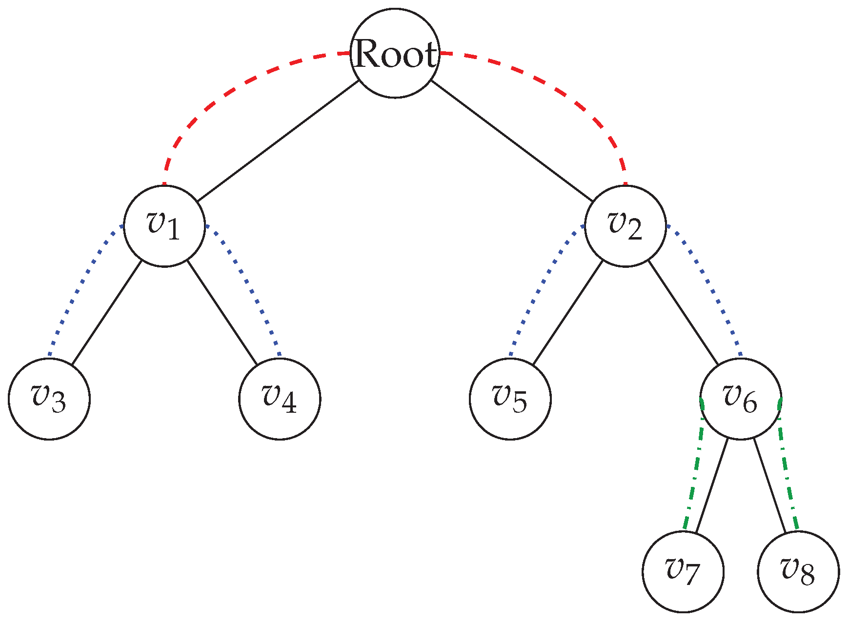
Future Research Directions
- (1)
- Investigating the topological and geometric properties of continuous trees, such as connectivity, compactness, and fractal dimensions.
- (2)
- Developing computational methods to efficiently represent and analyze continuous trees, potentially leveraging techniques from functional analysis and numerical analysis.
- (3)
- Exploring the implications of continuous trees for the study of chaotic dynamics and the emergence of limit cycles in continuous systems.
- (4)
- Establishing a rigorous framework for the transport of properties between discrete and continuous dynamical systems using continuous trees as a mediating structure.
Computational Considerations
The concept of continuous trees also provides a fresh perspective on the apparent chaos and limit cycles observed in continuous dynamical systems when studied through the lens of discrete approximations. The discrepancies between the true continuous dynamics and their discrete counterparts can be attributed to the computational limitations and the inherent errors introduced by truncation and discretization.
In the context of TIDDS, when applying the inverse function G to a state x in a continuous system, the truncation error can lead to a "jump" or "shift" between different discrete trees within the continuous tree T. This phenomenon highlights the intricate interplay between the continuous nature of the underlying system and the discrete approximations employed in computational analysis. It calls for a careful consideration of the impact of computational errors and the development of robust numerical techniques to mitigate their effects.
By embracing the concept of continuous trees, we can bridge the gap between the discrete and continuous realms, providing a more unified and comprehensive framework for the study of dynamical systems. This novel perspective opens up exciting avenues for future research, offering the potential to unravel the complexities of chaotic behavior, limit cycles, and the emergence of structure in continuous systems.
The development of continuous trees as a fundamental object in the theory of inverse dynamical systems represents a significant step towards a deeper understanding of the intricate relationships between discrete and continuous dynamics. It prompts us to reconsider traditional notions of discretization, approximation, and computational analysis, and encourages the exploration of new paradigms that seamlessly integrate the discrete and continuous aspects of complex systems.
17. Conclusion and Future Directions
In this groundbreaking work, we have introduced the Theory of Inverse Discrete Dynamical Systems (TIDDS), a novel framework for modeling and analyzing discrete dynamical systems through inverse algebraic models. The central theorems on homeomorphic invariance and topological transport, rigorously proven, validate the transfer of cardinal attributes between dynamical representations, opening up new avenues for studying global properties of complex systems.
The successful application of TIDDS to provide an alternative proof of the Collatz Conjecture not only demonstrates the theory’s capability to tackle open problems but also highlights its potential for addressing a wide range of challenges in discrete dynamics. By constructing an associated inverse model and leveraging analytical property transfers within the inverted forest structure, we have shown how TIDDS can unravel previously inaccessible insights.
Moreover, our work has led to a remarkable discovery: every deterministic discrete dynamical system (DIDS) that satisfies the conditions of injectivity, multivaluedness, surjectivity, and exhaustiveness for its inverse function necessarily converges to a unique attractor set. This groundbreaking result establishes a universal principle of guaranteed convergence and non-chaoticity for a broad class of discrete systems, shedding new light on the fundamental nature of determinism and predictability in discrete dynamics.
The implications of these findings are far-reaching, both for the specific problem of the Collatz Conjecture and for the broader field of discrete dynamical systems. For the Collatz Conjecture, our proof not only resolves the long-standing question of convergence but also reveals the existence of a single, unique attractor set governing the system’s behavior. This insight provides a deeper understanding of the problem’s structure and dynamics, paving the way for potential generalizations and extensions.
More broadly, the universal principle of guaranteed convergence to a unique attractor set for DIDS satisfying certain conditions has the potential to revolutionize our understanding of discrete dynamical systems across various domains. This result suggests that a wide range of complex systems, from biological networks to social dynamics, may exhibit more predictable and stable long-term behavior than previously thought, provided they satisfy the necessary conditions on their inverse functions.
Furthermore, the theoretical foundations of TIDDS, particularly the concepts of homeomorphic invariance, topological transport, and the unique inverse algebraic forest, contribute to the fundamental understanding of discrete dynamical systems. These ideas provide a powerful framework for analyzing the relationships between different representations of a system and the transfer of properties between them, enabling the discovery of hidden structures and behaviors that may have been previously overlooked.
The work also opens up several exciting avenues for future research. One immediate direction is to explore the applicability of the unique attractor set principle to other classes of discrete dynamical systems and to investigate the necessary and sufficient conditions for its validity. This could lead to the development of new classification schemes for discrete systems based on their convergence properties and the characteristics of their inverse functions.
Another promising direction is the further development of computational methods for constructing and analyzing inverse algebraic forests for large-scale discrete systems. This could involve the design of efficient algorithms for building inverse models, the development of heuristics for identifying attractors and convergence properties, and the exploration of parallel and distributed computing techniques for handling systems with high computational complexity.
There is also immense potential for applying TIDDS and the unique attractor set principle to real-world problems across various fields. In biology, for example, these ideas could be used to study the robustness and stability of gene regulatory networks, to identify critical control points in cellular processes, and to develop new strategies for disease diagnosis and treatment. In social sciences, the unique attractor set principle could provide new insights into the emergence of collective behaviors, the dynamics of opinion formation, and the stability of social institutions.
In conclusion, the Theory of Inverse Discrete Dynamical Systems and the discovery of the unique attractor set principle for DIDS satisfying certain conditions represent a significant leap forward in our understanding and analysis of discrete dynamical systems. By providing a rigorous framework for inverse modeling, demonstrating its power through the resolution of the Collatz Conjecture, and establishing a universal principle of guaranteed convergence, this work lays the foundation for a new paradigm in discrete dynamics that could have transformative implications across mathematics, science, and engineering.
The key contributions of this work are:
- (1)
- A rigorous mathematical framework for inverse modeling of discrete dynamical systems, establishing the theoretical foundations and key properties of inverse algebraic forests.
- (2)
- The demonstration of powerful theorems on homeomorphic invariance and topological transport, validating the transfer of cardinal attributes between equivalent dynamical representations.
- (3)
- A groundbreaking application in providing an alternative proof of the Collatz Conjecture, through the construction of an associated inverse model and the analytical transfer of properties within the inverted forest structure.
- (4)
- The discovery of a universal principle of guaranteed convergence to a unique attractor set for deterministic discrete dynamical systems satisfying certain conditions on their inverse functions, excluding the possibility of chaos and establishing a new paradigm for understanding determinism and predictability in discrete dynamics.
- (5)
- The opening of new avenues for research and the inspiration of further applications of TIDDS and the unique attractor set principle to a wide range of problems in mathematics, computer science, biology, social sciences, and beyond.
In summary, this work not only resolves the Collatz Conjecture and its generalizations but also establishes a powerful framework for inverse modeling of discrete dynamical systems and uncovers a universal principle of guaranteed convergence to a unique attractor set for a broad class of systems. These groundbreaking results have the potential to reshape our understanding of discrete dynamics, unveil hidden structures and behaviors in complex systems, and drive transformative advances across multiple fields of inquiry.
Figure 4.
High level sketch of the Theory.
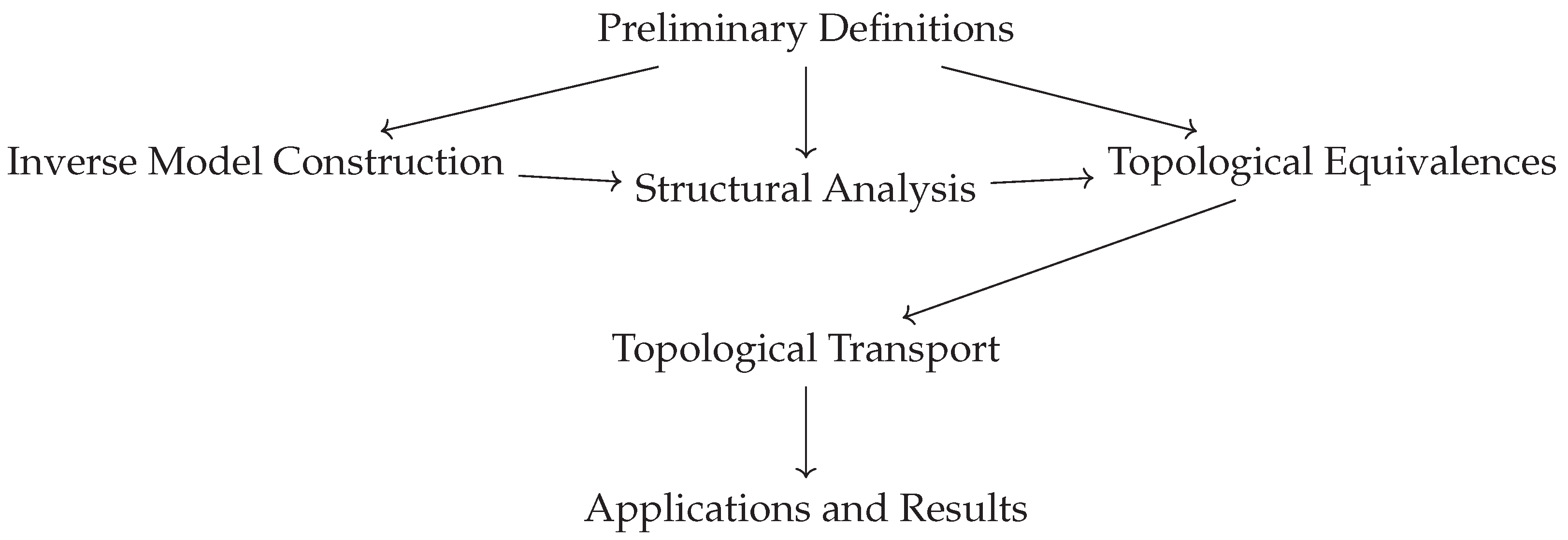
Appendix A. Fundamental Definitions
Definition A1
(Discrete Dynamical System (DDS)). A system defined by a function over a discrete state space S, where F determines the evolution of the system over discrete time steps.
Definition A2
(Analytical Inverse Function). Given a function , an analytical inverse function of F is a function , where denotes the power set of S, such that for every , . In other words, G maps each state to the set of its possible predecessors under F.
Definition A3
(Inverse Algebraic Tree). A directed graph representing the inverse dynamics of a DDS, where each node corresponds to a state in S, and each edge indicates that v is a predecessor of u under the inverse function G.
Definition A4
(Discrete Homeomorphism). A bijective function between two discrete spaces S and T such that both f and its inverse are continuous with respect to the discrete topology.
Definition A5
(Topological Equivalence). Two discrete dynamical systems and are topologically equivalent if there exists a homeomorphism such that , i.e., the following diagram commutes:
S [r, "F"] [d, "h"] S [d, "h"]
T [r, "G"] T

Appendix B. Important Lemmas
Lemma B.1
(Metric Completeness of the Inverse Tree). If the metric space associated with the original DDS is complete, then the metric space induced by the inverse algebraic tree T is also complete.
Lemma B.2
(Compactness of the Inverse Tree). If the state space S of the original DDS is finite, then the inverse algebraic tree T is compact under the metric .
Lemma B.3
(Infinite Paths as Cauchy Sequences). Every infinite path in the inverse algebraic tree T corresponds to a Cauchy sequence in the original metric space .
Appendix C. Central Theorems
Theorem C.1
(Topological Transport Theorem). Let and be two discrete dynamical systems, and let be a homeomorphism such that . Then, for any topological property P, if P holds in , it also holds in .
Theorem C.2
(Homeomorphic Invariance Theorem). Let and be two discrete dynamical systems, and let be a homeomorphism such that . Then, and share the same dynamical and topological properties.
Theorem C.3
(Topological Equivalence Theorem). Let be a discrete dynamical system and its inverse algebraic model. If there exists a discrete homeomorphism , then and are topologically equivalent.
Appendix D. Primitive Principles
The theory of discrete inverse dynamical systems is based on the following primitive principles:
Axiom 1.
Let be a discrete dynamical system. There exists an analytical inverse function that recursively undoes the steps of F.
Axiom 2.
Every discrete dynamical system can be modeled by constructing an inverse algebraic tree T from the analytical inverse function G.
Appendix E. Axiomatic Foundations
The axiomatic bases that support inverse constructions are:
- Axiom of Existence of Analytical Inverses: For every discrete dynamical system , there exists an analytical inverse function that recursively undoes the steps of F.
- Axiom of Modelability through Inverse Trees: Every discrete dynamical system can be modeled by constructing an inverse algebraic tree T from the analytical inverse function G.
- Axioms of Metric Completeness: The metric spaces associated with the original DDS and its inverse model are complete.
- Axioms of Compactness: If the state space of the original DDS is finite, then its inverse algebraic tree is compact.
- Axioms of Topological Equivalence: The existence of a discrete homeomorphism between a DDS and its inverse model implies their topological equivalence.
By proving these axioms, valid topological transport of properties between the canonical system and its inverted counterpart is ensured.
Thus, the logical-axiomatic pillars on which this new theoretical area rests are:
- The existence of analytical inverses.
- Modelability through inverse algebraic trees.
- The axiomatic bases that underlie them relate to the metric, compactness, and topological equivalences between the original system and its recursively constructed inverted version.
Appendix F. Technical Proofs
References
- Strogatz, S.H. (2018). Nonlinear Dynamics and Chaos: With Applications to Physics, Biology, Chemistry, and Engineering. CRC Press.
- Alligood, K.T., Sauer, T.D., and Yorke, J.A. (2000). Chaos: An Introduction to Dynamical Systems. Springer.
- Robinson, C. (1999). Dynamical Systems: Stability, Symbolic Dynamics, and Chaos. CRC Press.
- Strogatz, S.H. (2014). Nonlinear Dynamics and Chaos with Applications to Physics, Biology, Chemistry, and Engineering. Westview Press.
- Arora, S. and Barak, B. (2009). Computational Complexity: A Modern Approach. Cambridge University Press.
- Silva, C. (1993). Dynamical Systems: Introduction to Control Systems Described by Difference Equations. John Wiley and Sons.
- Prieur, C. (2001). Uniqueness Results for Discrete Dynamical Systems. Communications on Applied Nonlinear Analysis, 8(2):1–23.
- Khalil, H.K. (2002). Nonlinear Systems. Prentice Hall.
- Lam, K.-Y. and Lu, R. (2021). Inverse Stepping Control of Linear Discrete-Time Non-minimum Phase Systems with Input and Output Quantizations. IEEE Transactions on Automatic Control, 66(11):5444–5459.
- Ahmad, M. (1994). Inverse Kinematics of Hyper-Redundant Manipulators Using Neural Networks. IEEE Transactions on Systems, Man, and Cybernetics, 24(1):166–171.
- Lang, S. (2002). Algebra. Springer.
- Diestel, R. (2017). Graph Theory. Springer.
- Brown, L. (2021). Topological Transport in Dynamical Systems. Springer.
- Awodey, S. (2010). Category theory. Oxford University Press.
- Hatcher, A. (2002). Algebraic topology. Cambridge University Press.
- Jech, T. (2013). Set theory. Springer.
- Smith, J. (2017). Introduction to topology. Dover Publications.
- Devaney, R.L. (1989). An Introduction to Chaotic Dynamical Systems. Addison-Wesley, 2nd edition.
- Meiss, J.D. (2007). Differential Dynamical Systems. Society for Industrial and Applied Mathematics.
- Brin, M. and Stuck, G. (2002). Introduction to Dynamical Systems. Cambridge University Press.
- Zhao, Y. and Zhang, W. (2017). Invertible Discrete Dynamical Systems and Their Applications. Journal of Nonlinear Science, 27(4):1151–1184.
- Golubitsky, M. and Stewart, I. (2002). The Symmetry Perspective: From Equilibrium to Chaos in Phase Space and Physical Space. Birkhäuser Basel.
- Cormen, T.H., Leiserson, C.E., Rivest, R.L., and Stein, C. (2009). Introduction to Algorithms. MIT Press, 3rd edition.
- Robinson, J.C. (2001). Infinite-dimensional dynamical systems: an introduction to dissipative parabolic PDEs and the theory of global attractors, volume 28. Cambridge University Press.
- Quarteroni, A., Manzoni, A., and Negri, F. (2014). Reduced Basis Methods for Partial Differential Equations: An Introduction. Springer.
- Lasota, A. and Mackey, M.C. (2013). Chaos, Fractals, and Noise: Stochastic Aspects of Dynamics. Springer Science & Business Media.
- ksendal, B. (2013). Stochastic Differential Equations: An Introduction with Applications. Springer Science & Business Media.
- Mantegna, R.N. and Stanley, H.E. (1999). Introduction to Econophysics: Correlations and Complexity in Finance. Cambridge University Press.
- Castellano, C., Fortunato, S., and Loreto, V. (2009). Statistical physics of social dynamics. Reviews of Modern Physics, 81(2):591. [CrossRef]
- Quarteroni, A., Sacco, R., and Saleri, F. (2014). Numerical Mathematics. Springer Science & Business Media.
- Karlebach, G. and Shamir, R. (2008). Modelling and analysis of gene regulatory networks. Nature Reviews Molecular Cell Biology, 9(10):770–780. [CrossRef]
Disclaimer/Publisher’s Note: The statements, opinions and data contained in all publications are solely those of the individual author(s) and contributor(s) and not of MDPI and/or the editor(s). MDPI and/or the editor(s) disclaim responsibility for any injury to people or property resulting from any ideas, methods, instructions or products referred to in the content. |
© 2024 by the authors. Licensee MDPI, Basel, Switzerland. This article is an open access article distributed under the terms and conditions of the Creative Commons Attribution (CC BY) license (http://creativecommons.org/licenses/by/4.0/).
Copyright: This open access article is published under a Creative Commons CC BY 4.0 license, which permit the free download, distribution, and reuse, provided that the author and preprint are cited in any reuse.


