
Submitted:
10 October 2023
Posted:
11 October 2023
You are already at the latest version
Abstract
Water conflicts have been a significant issue in Brazil, especially in the Sao Francisco River basin. Subseasonal forecasts, up to a 60-day forecast range, can provide information to support decision-makers in managing water resources in the river basin, especially before drought events. Predictability in the subseasonal forecasts range is a research topic as this range contains mixed dependence on weather and seasonal phenomena. Numerical models may inherit this mixed dependence on their skills. The objective of this paper is to evaluate the Eta Model simulations to reproduce the drought events between the years 2011 and 2016. Two sets of 60-day simulations were produced; one started in September (SO) and the other in January (JF) each year. These months were chosen to evaluate the model skill to reproduce the onset and the middle of the rainy seasons in Central Brazil, where the Upper Sao Francisco River is located. The SO simulations reproduced the observed spatial distribution of precipitation but underestimated the amounts. Precipitation errors exhibit large variability across the subbasins. The JF simulations also reproduced the observed precipitation distribution but overestimated it in the Upper and Lower subbasins. The JF simulations better captured the interannual variability of precipitation. The 60-day simulations were discretized in six 10-day accumulations to assess the intra-monthly variability. They showed that simulations can capture the onset of the rainy season and the small amounts of the rainy months that occurred in these severe drought years.
Keywords:
Climate extremes
; transition season
; rainy season
; model errors
; extended range
1. Introduction
The Sao Francisco River in Brazil plays an important socioeconomic role due to its long north-south extension and the high water demand for the various activities in the basin. Major hydropower plants and intensive agriculture activities are established in the basin. However, the basin is located in a region with remarkable climate variability, directly affecting its hydrological regime and water availability. The occurrence of climatic extremes requires constant monitoring of the water levels of the basin and the management of water access. Accurate information on water availability is fundamental for implementing actions to reduce conflicts in water usage.
The numerical atmospheric models are essential for producing information for managing water resources. Using these models at subseasonal ranges may provide information, such as precipitation, temperature, radiation, humidity, wind, and evapotranspiration, helpful in planning actions in various socioeconomic sectors such as energy, agriculture, and water supply. However, these model simulations may have limitations related to the dependence on the boundary conditions. It is known that after approximately two weeks, the predictability of the individual weather systems is significantly reduced and that the predictability at the seasonal scale of average weather conditions can only increase in the presence of forcing from the boundary conditions [2]. Model simulations are more likely to have higher skill in situations of high predictability. Therefore, investigating the level of the forecast skill is crucial for making the model information useful. For this reason, it is necessary to evaluate the subseasonal forecasts so that they can be applied in different research.
Atmospheric General Circulation Models (AGCM) are generally used in weather and climate forecasts. However, it may need to be improved for the coarse grid and the discrepancy between the climate and hydrological modeling. Higher spatial resolution information is more suitable for dealing with local problems [1]. The Regional Climate Models (RCMs) aim to refine the coarse grid of the AGCMs for a specific region of interest. The Eta model ([4,5,6,7]) has been applied in the category of weather, seasonal climate forecasts, paleoclimate studies, and climate change projections in Brazil, producing information for several applications.
This paper aims to evaluate the 5-year mean subseasonal simulations of the Eta regional model from 2011 to 2016 and assess the usefulness of the information to support decision-making in water resources conflicts in the Sao Francisco River basin.
2. Materials and Methods
2.1. Study area
The study area is the region of the Sao Francisco River basin (SF) (Figure 1). The SF river basin is one of the major rivers in Brazil. It is approximately 2,700 km long and discharges an average flow of 2,810 m³/s into the Atlantic Ocean [8]. Its watershed has an area of 639.219 km², with different topographic and geomorphic features, and a population of about 13 million. The basin is commonly divided into four subbasins: Upper, Middle, Sub-Middle, and Lower (Figure 1). The lowest two river courses are located in the Semiarid region, where dry periods can be prolonged and become droughts.
The Sao Francisco River basin allows multiple water uses, such as hydroelectricity, agriculture, navigation, fishing and aquaculture, human and industrial supplies, flood control, recreation, and tourism. However, the wide variation in water availability throughout the basin and through the seasons makes it difficult to plan an efficient water allocation. Interannual variability in water availability may be partly related to climate variability, characterized by extremely rainy and dry years. Potential conflicts in this basin between the energy and agricultural sectors have been alerted [10], such as the allocation of water from the Sobradinho reservoir for power generation and irrigation practices. The conflicts were aggravated, especially in the Semiarid between 2011 and 2016, with rainfall below normal levels in the basin.
Although water availability in the basin generally meets multiple uses, the increasing demand for water resources leads to significant and occasional conflicts. According to [12], variability in the river flows and lake levels depends on precipitation variability in accumulated volume and intensity.
Different climate regimes are found in the Sao Francisco Basin (SF) due to its long north-south extension and the topographic differences. In the Upper SF, the climate varies from subtropical humid with dry winter and hot summer and temperate summer, Cwa and Cwb in Koppen's classification. In the Middle SF, the tropical climate with dry winter, Aw, predominates. The Lower SF is predominately semiarid with some small patches of tropical, dry summer (Alvares et al., 2013)
2.2. Eta model
The Eta model is a grid point limited area model, which represents the topography in steps, using the eta vertical coordinate [4]. The approximately horizontal surfaces of the eta coordinate reduce the errors in calculating the horizontal derivatives near topography, which are errors commonly found in terrain-following coordinates, as the gradient force, resulting in a better representation of regions of steep topography. The Eta is a comprehensive model with full dynamics and physics.
The model has received updates [5] since the operational version used at the National Centers for Environmental Prediction (NCEP) [6] [7] as the cut-cells. The model equations are solved on the Arakawa E-grid. The time integration is split-explicit, using the forward-backward and Euler-backward schemes modified by [14]. The horizontal advection follows the Arakawa approach [15], and the vertical advection uses the piecewise linear scheme, which makes it a full finite volume model. The model physics package of this version applies the Betts-Miller scheme [16] to produce convective precipitation and the Zhao scheme [17] for grid-scale precipitation. The longwave component of the radiation is solved by [18], and the shortwave component is solved by [19]. The surface layer is based on the Monin-Obukhov similarity theory and Paulson’s [20] stability functions. Land surface processes are treated using the NOAH scheme [21].
Several studies evaluated the Eta model skills in different configurations [1,22,23,24,25,26,27,28,29,30]. Some works have investigated the Eta model skills over some parts of the Sao Francisco River basin on a seasonal scale [31,32,33]. [31] used seasonal forecasts of the Eta model between November and February from 2001 to 2010. The authors concluded that the model presented difficulties in reproducing the precipitation interannual variability in the Upper SF basin. Some studies also evaluated the Eta model in Southeast Brazil, which is known for its low predictability. The recent studies of [24] presented the Eta model skills in subseasonal forecasts. In this context, it is essential to evaluate the climatic variability of the Eta prediction to promote management that includes the investigation of climatic variability and its effects on the water availability of the basin. Results from the Eta model subseasonal forecast can assist in decision-making on water use allocation based on 1 to 2-month lead time. Therefore, early knowledge of periods of deficit or excess rainfall allows better planning on the use of water resources.
Eta model simulations on the subseasonal time range were generated for the 60-day integration, with 20-km horizontal resolution. The model's initial conditions were obtained from the Climate Forecast System Reanalysis (CFSR) reanalysis [36]. The integrations start on September 1st and January 1st to evaluate the model's accuracy at the onset and the middle of the rainy seasons in Brazil, respectively. These two simulation runs will be referred to as SO (September-October) and JF (January-February) runs. The first run contains the onset of the rainy season and the second, the middle of the rainy season.
2.3. Observational data
The evaluation compares the Eta precipitation simulation against the Climate Prediction Center Morphing (CMORPH) precipitation data. The CMORPH [37] data presents a horizontal resolution of 8 km.
Despite the advantages of details provided by regional model simulations, systematic errors persist. These systematic errors may be associated with the forcing of the global climate model added to those inherent in the regional model's representation of physical processes. The performance of subseasonal simulation was evaluated with metrics such as linear correlation, mean absolute error (MAE), and mean error (ME).
3. Results and discussion
The simulations of precipitation variability over the 5-year mean are assessed. The mean of the 60-day simulation was discretized into 10-day simulations to evaluate intra-monthly variations: from dry-to-wet transition (SO) and the middle of the rainy seasons (JF), and referred to as D1, D2, D3, D4, D5, D6 periods.
3.1. Precipitation pattern
In SO, the Eta generally simulates less precipitation compared to CMORPH in the SF (Figure 2). However, in the Lower SF, Eta simulates precipitation in the Northeast Brazil coastal areas, where CMORPH indicates little or no precipitation. This region is known as a region of high predictability. In the Upper SF, the model introduces precipitation in D5, while CMORPH shows precipitation from D2.
Over the Sao Francisco (SF) River basin, the JF simulations reproduce the CMORPH precipitation pattern, with larger accumulated amounts in the Upper SF and Lower SF (Figure 3). The JF simulation reproduce the precipitation pattern better than the SO simulation.
The presence of precipitation simulated in the Northeast Brazil coast may suggest an overestimate by the model. However, Lima et al. (2012) showed the poor performance of satellite precipitation estimates over Northeast Brazil, especially in estimating stratiform rainfall, which occurs frequently over Northeast Brazil. Lima et al. (2012) the CMORPH products against other rainfall estimation methods in the summer (from December to February) between 2009 and 2011 in South America. They concluded that the models with the best performances were 3B42RT and CMORPH, mainly for the South and Southeast of Brazil. Due to the CMORPH limitation in estimating precipitation in Northeast Brazil, other sources of data will be considered for validating precipitation in this coastal area, especially in June and July, its rainy season.
3.2. Interannual variability
The Eta simulation performance is evaluated over the 4 major sub-basins of the Sao Francisco (SF) river: the Upper SF, Middle SF, Sub-Middle SF, and Lower SF. Figure 4 shows the precipitation for SO simulations, starting in September (2011 to 2015), and JF simulations, starting in January (2012 to 2016).
In the SO simulations, the model approximately reproduces the decrease and increase in the magnitude of the 60-day accumulated total precipitation. The simulation of the interannual variability could be improved. The small amounts of precipitation in 2014 and 2015 hinted at the delay in the onset of the rainy season in these years. Both the Eta model and the CMORPH indicate that the subbasin of the smallest rainfall volume is the Sub-Middle SF. In the Lower subbasin, CMORPH data show no precipitation, but the runs show amounts of about 100 mm/60 days. This overestimate is partly due to CMORPH limitations as discussed in the previous section.
Both SO runs and the CMORPH data indicate that the highest precipitation volumes occur over the Upper SF and the Middle SF, and the lowest volumes occur over the Sub-Middle SF.
In the JF simulations, large precipitation volumes occur in the middle of the rainy season. The JF simulations generally reproduce the interannual variability shown in the CMORPH estimate. The JF simulations captured the strong reduction of precipitation in 2014 when the rainfall was extremely below the climatology [40] [41]. The Eta simulations captured well the precipitation decrease in 2014 and 2015 and the increase in 2016. The Upper subbasin receives the highest rainfall, while the Sub Middle receives the lowest.
In a 60-day accumulation, the simulations perform better for rainy months JF than for the transition from dry to wet months SO. In addition, these results show the different precipitation regimes across the sub-basins. These differences impose some difficulties on the model simulations over the SF basin.
3.3. Intra-monthly variability
The intra-monthly variability is shown through boxplots of every 10-day accumulated precipitation from the SO (Figure 5) and JF (Figure 6) simulations Clearly, the JF simulations have higher precipitation amounts than SO.
In the Upper SF, the SO simulation showed some limitations in representing the intra-monthly variability of the first three 10-day simulations, D1, D2, and D3. On the other hand, these simulations captured correctly the variability of the last three 10-day simulations, D4, D5, and D6. The increase of the precipitation median in D5 and D6 in the Upper and Middle subbasins, shown by the CMORPH data, is the indication of the onset of the rainy season, which was captured by the Eta simulations. The simulations also captured the lack of precipitation in all 10-day accumulations in the Sub-Middle subbasin. However, at the Lower subbasin, the simulation overestimated the precipitation, which may be a partial error from CMORPH data as discussed previously.
In the Middle SF, the JF simulations captured the large spread in precipitation between the 25th and 75th percentiles in the D1-D3 and a decrease in the spread and in the amount of 10-day accumulated precipitation. However, in Sub-Middle SF, the simulations generally underestimated the accumulated precipitation, except for the D3, when they overestimated the precipitation. The CMORPH data places D2 as a rain peak, while the Eta simulations peak in D3, which indicates a slight delay. Finally, despite underestimating the precipitation in the Lower SF, the Eta presented consistent values when compared to CMORPH.
3.4. Simulations´ skill
The evaluation of the Eta model skill to simulate precipitation in the Sao Francisco basin was evaluated using Linear Correlation (Figure 7), Mean Absolute Error (Figure 8), and Mean Error (Figure 9).
The highest correlations between Eta and CMORPH precipitation are shown in JF than in SO (Figure 7). In SO, correlations become small or even negative from D2. In JF simulations, it can also be seen that the Eta and CMORPH precipitation series are strongly to moderately correlated from the D1 up to D4. In both SO and JF runs, the highest correlations are found in the Middle SF. The model indicated difficulty representing the Lower SF, especially during the SO runs, this may be partly due to CMORPH limitations in this subbasin.
Although the correlation was low in SO simulations, the mean absolute errors (MAE) of precipitation are smaller in SO than in JF, given that the accumulated precipitation is smaller in SO than in JF (Figure 8). D5 is the 10-day simulation with the highest MAE and the most significant rainfall in most of subbasins. Considering the entire SF basin, the MAE reaches 16.56 mm and up to 27.05 mm in the Upper SF. In JF, the highest MAE are found in D2 and D3, the periods with the most significant rainfall. For example, the highest MAE reaches about 39.14 mm in the Upper SF, in D2.
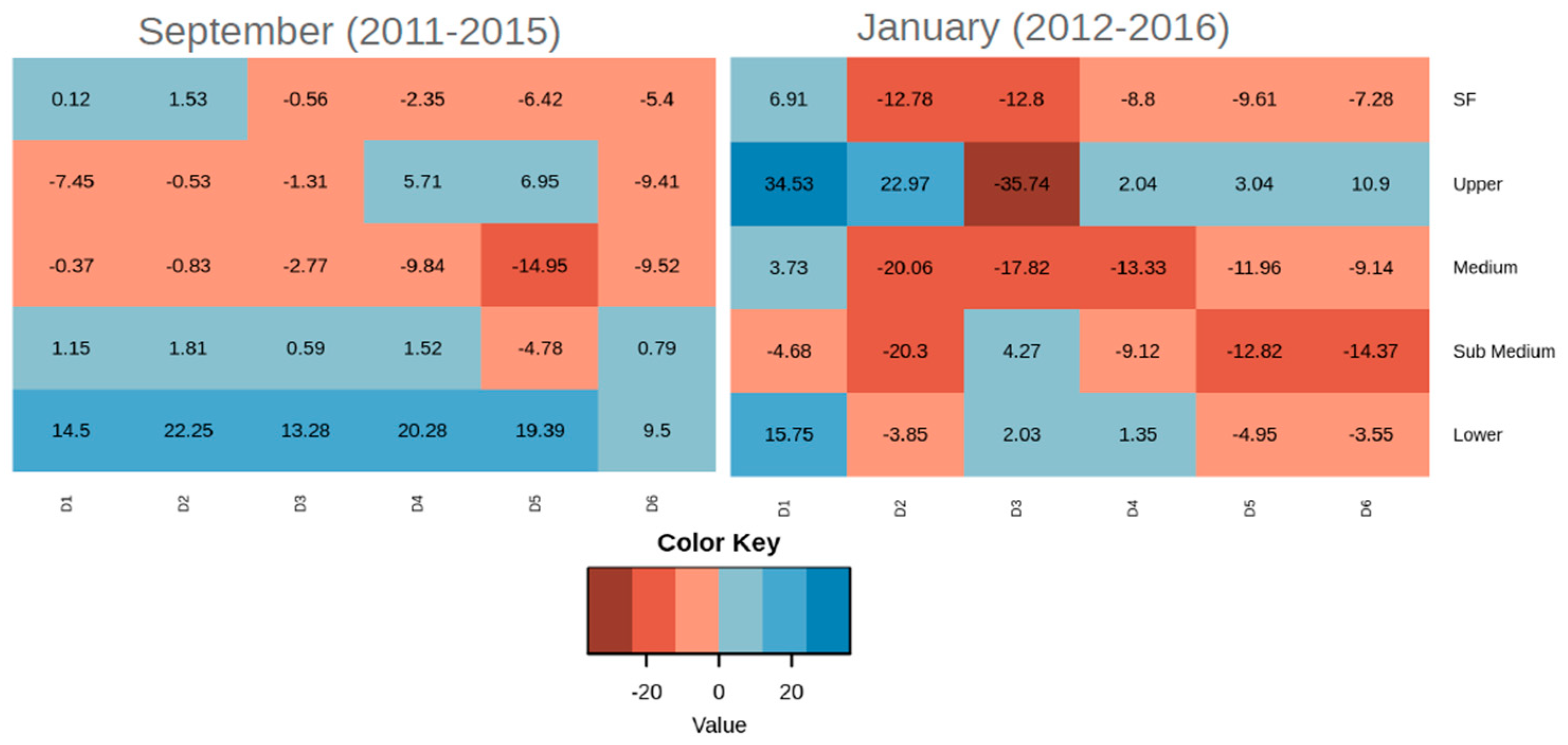
The Mean Error (ME) estimates help to indicate whether simulations overestimate or underestimate precipitation in each sub-basin and at different simulations (Figure 9).
Considering the entire SF basin, the SO simulations overestimate precipitation in the D1 and D2 and underestimate in the D3, D4, D5, and D6. The precipitation simulations in the Middle SF contribute mostly to the underestimation of the SF basin, whereas the precipitation simulations in the Sub-Middle and the Lower SF contribute to the overestimation of the basin from D1 to D6, in general. Generally, the largest ME in the SO simulation occurs in D5 in the Sub-Middle SF. However, in D6, errors decrease, indicating usefulness in this range of the simulation.
In JF simulations, ME indicates an underestimation of precipitation over the SF basin, except in D1. As in SO, in JF, the Middle SF contributes significantly to the underestimation. In the Upper SF, precipitation is generally overestimated, especially in D1, with errors that reach 34.53 mm. Precipitation is mostly underestimated in the Sub-Middle subbasin, and slightly less in the Lower SF.
From the results presented, the subseasonal simulations for the SF basin show some limitations in the transition months. Some aspects that may contribute to the model errors are the complex topography, heterogeneous vegetation, and general climate conditions in the river basin. In general, precipitation in the Upper and Middle SF subbasins were better simulated, although still exhibiting relatively large errors.
4. Conclusions
5-year mean subseasonal simulations were generated from the Eta model driven by CFSR conditions. The 60-day simulations started in September, SO, from 2011 to 2015 and January, JF, from 2012 to 2016, and were assessed the discretized six 10-day precipitation outputs.
In the SO runs, the Eta model simulated lower precipitation volumes than CMORPH. However, Eta simulated precipitation in Lower SF, coastal regions, where CMORPH indicated little or no precipitation. In the Upper SF, the Eta model produced rain from D3 and CMORPH from D1, which shows a model's difficulty in representing precipitation in transitional months.
The 10-day simulations show that Eta produced higher precipitation rates in the Upper and Lower SF, while CMORPH showed higher precipitation rates in the Upper and Middle SF. Both Eta and CMORPH showed maximum rainfall at D5 as an indication of the onset of the rainy season. Considering the entire SF basin, the simulations reproduced the rainfall distribution over the 60 days of simulations.
Despite the low correlation, the SO runs have a small MAE due to the small precipitation volume. Considering the entire SF basin, the Eta overestimates D1 and D2 and underestimates D3, D4, D5, and D6. However, errors vary strongly along the basin. In Middle SF, precipitation is underestimated, while in Lower SF, it is overestimated.
In the JF simulations, precipitation is overestimated in the Lower SF, on the northeast coast, while CMORPH shows no precipitation. However, in the Upper SF, the Eta simulations show a similar rainfall distribution as CMORPH, with higher precipitation values. The JF simulations reproduce the annual variability better than the SO simulations.
Both Eta and CMORPH indicate that in the SF basin, the highest rainfall occurs in the first three 10-day simulations, D1, D2, and D3. In the Upper SF, the model has limitations in the first three 10-day simulations and then simulates well in the last three. In Middle SF, Eta reproduces the CMORPH precipitation distribution pattern well, with the highest precipitation values in the first three 10-day simulations. In the Lower SF, although underestimated, the precipitation simulated by Eta was consistent with CMORPH. The highest correlation values are found in the JF simulations. The highest correlations and the smallest MAE are generally found in D1 and D4. A variable error pattern is identified at the Upper SF, with overestimation and underestimation according to the 10-day simulation, while in the other three subbasins, underestimation is identified. The largest ME is found in JF simulations, which are the months of higher rainfall compared to SO simulations.
The present research contributes to assessing subseasonal scale simulations using a Regional Climate Model. This type of assessment has been more extensively applied to Global Climate Models. The Eta Model simulations showed good performance at this scale. However, there are some limitations in the assessment applied that should be kept in mind. The evaluation was based on the CMORPH data, whose resolution is higher than the simulations model. For this reason, some extreme events may not be simulated. In addition, the study region where the SF basin is located has low predictability.
Further modeling studies are required, including updates of soil maps, vegetation, and adjustments to rainfall production. Future studies will incorporate these improvements, and bias removal may also be included. Therefore, this research is a critical step to indicate subbasins where the model simulation needs to be improved and provide initial information to support water allocation in the region.
Author Contributions
Conceptualization, all authors.; methodology, software, NCRF; validation, all authors; formal analysis, investigation, data curation, writing—original draft preparation, NCRF; writing—review and editing, all authors; visualization, NCRF.; supervision, project administration, SCC.; funding acquisition, NCRF, SCC. All authors have read and agreed to the published version of the manuscript.
Funding
This research was funded jointly by the Agência Nacional de Águas e Abastecimento and the Coordenação de Aperfeiçoamento de Pessoal de Nível Superior Project ANA/CAPES no.88881.144894/2017-01. SCC thanks Conselho Nacional de Desenvolvimento Científico e Tecnológico (CNPq) for grant 312742/2021-5. MLRSS thanks CNPq/INPE/PIBIC for the grant 800353/2018-8. NCRF thanks CAPES for grant no. 88887.351539/2019-00.
Conflicts of Interest
The authors declare no conflict of interest.
References
- Alvares, C.A.; Stape, J.L.; Sentelhas, P.C.; Moraes, G.J.L.; Sparovek, G. Köppen’s climate classification map for Brazil. Meteorol. Z. 2013, 22, 711–728. [Google Scholar] [CrossRef] [PubMed]
- Rodwell, M.J.; Doblas-Reyes, F.J. Medium-Range, Monthly, and Seasonal Prediction for Europe and the Use of Forecast Information. J. Clim. 2006, 19, 6025–6046. [Google Scholar] [CrossRef]
- Collischonn, W.; Tucci, C. Simulação hidrológica de grandes bacias. Revista Brasileira de Recursos Hídricos 2001, 6. [Google Scholar]
- Mesinger, F. A blocking technique for representation of mountains in atmospheric models. Riv. Meteor. Aeronaut. 1984, 195–202. [Google Scholar]
- F. Mesinger, S. Chou, J. Gomes, D. Jovic, L. Lazic, A. Lyra and I. Ristic, "An upgraded Version of the Eta Model," in European Geosciences Union (EGU) General Assembly 2011 (Vol. 13, pp. EGU2011-3753)., 2011.
- Black, T.L. The New NMC Mesoscale Eta Model: Description and Forecast Examples. Weather. Forecast. 1994, 9, 265–278. [Google Scholar] [CrossRef]
- Mesinger, F.; Janjić, Z.I.; Ničković, S.; Gavrilov, D.; Deaven, D.G. The Step-Mountain Coordinate: Model Description and Performance for Cases of Alpine Lee Cyclogenesis and for a Case of an Appalachian Redevelopment. Mon. Weather. Rev. 1988, 116, 1493–1518. [Google Scholar] [CrossRef]
- J. G. Gondin Filho, K. T. Formiga, R. X. Duarte and M. R. Sugai, "Análise da cheia de 2004 na bacia do rio São Francisco," in Simpósio Brasileiro de Desastres Naturais, Florianopolis, 2004.
- L. M. C. da Silva and R. A. Monteiro, "Outorga de direito de uso de recursos hídricos: uma das possíveis abordagens.," Gestão de águas doces. Rio de Janeiro: Interciência., 2004.
- ANA, "PAE: PROGRAMA DE AÇÕES ESTRATÉGICAS PARA O GERENCIAMENTO INTEGRADO DA BACIA DO RIO SÃO FRANCISCO E DA SUA ZONA COSTEIRA.," GEF São Francisco: Relatório Final. 336 p., Brasília, 2004.
- C. M. Mascarenhas, Conflitos e gestão de águas: o caso da bacia hidrográfica do rio São Francisco., Dissertação (Mestrado em Desenvolvimento Sustentável)-Universidade de Brasília., 2008.
- Chiew, F.H.S. Estimation of rainfall elasticity of streamflow in Australia. Hydrol. Sci. J. 2006, 51, 613–625. [Google Scholar] [CrossRef]
- Janjic, Z.I.; Gerrity, J.P., Jr.; Nickovic, S. An Alternative Approach to Nonhydrostatic Modeling. Mon. Weather Rev. 2001, 129, 1164–1178. [Google Scholar] [CrossRef]
- Janjic, Z.I. Forward-backward scheme modified to prevent two-grid-interval noise and its application in sigma coordinate models. Contrib. Atmos. Phys. 1979, 52, 69–84. [Google Scholar]
- Janjić, Z.I. Nonlinear Advection Schemes and Energy Cascade on Semi-Staggered Grids. Mon. Weather. Rev. 1984, 112, 1234–1245. [Google Scholar] [CrossRef]
- Betts, A.K.; Miller, M.J. A new convective adjustment scheme. Part II: Single column tests using GATE wave, BOMEX, ATEX and arctic air-mass data sets. Quarterly Journal of the Royal Meteorological Society 1986, 112, 693–709. [Google Scholar]
- Zhao, Q.; Carr, F.H. A Prognostic Cloud Scheme for Operational NWP Models. Mon. Weather. Rev. 1997, 125, 1931–1953. [Google Scholar] [CrossRef]
- Schwarzkopf, M.D.; Fels, S.B. The simplified exchange method revisited: An accurate, rapid method for computation of infrared cooling rates and fluxes. Journal of Geophysical Research: Atmospheres 1991, 96, 9075–9096. [Google Scholar] [CrossRef]
- Lacis, A.A.; Hansen, J. A parameterization for the absorption of solar radiation in the earth's atmosphere. Journal of the atmospheric sciences 1974, 31, 118–133. [Google Scholar] [CrossRef]
- Paulson, C.A. The mathematical representation of wind speed and temperature profiles in the unstable atmospheric surface layer. Journal of Applied Meteorology 1970, 9, 857–861. [Google Scholar] [CrossRef]
- Ek, M.B.; Mitchell, K.E.; Lin, Y.; Rogers, E.; Grunmann, P.; Koren, V.; Tarpley, J.D. Implementation of Noah land surface model advances in the National Centers for Environmental Prediction operational mesoscale Eta model. Journal of Geophysical Research Atmospheres 2003, 108, D22. [Google Scholar] [CrossRef]
- S. C. Chou, N. C. R. Ferreira, M. L. Rocha, J. L. Gomes, C. Dereczynski and G. Sueiro, "From subseasonal to seasonal forecasts over South America using the Eta Model," Numerical weather, 2018.
- S. C. R. N. d. R. M. L. D. C. P. G. J. L. &. S. G. Chou, "From subseasonal to seasonal forecasts over South America using the Eta Model," Numerical Weather, 2018.
- S. C. Chou, N. Resende, M. L. da Rocha, C. P. Dereczynski, J. L. Gomes and G. & Sueiro, "From subseasonal to seasonal forecasts over South America using the Eta Model. In "NUMERICAL WEATHER AND CLIMATE MODELING: Beginning, now, and vision of the future”. Serbian Academy of Science and Arts, p. 7-11, 2018.
- Seluchi, M.E.; Chou, S.C. Evaluation of two Eta Model versions for weather forecast over South America. Geofísica Internacional 2001, 40, 219–237. [Google Scholar] [CrossRef]
- Seluchi, M.E.; Chou, S.C. Synoptic patterns associated with landslide events in the Serra do Mar, Brazil. Theor. Appl. Clim. 2009, 98, 67–77. [Google Scholar] [CrossRef]
- Seluchi, M.E.; Chou, S.C.; Gramani, M. A case study of a winter heavy rainfall event over the Serra do Mar in Brazil. Geofísica Internacional 2011, 50, 41–56. [Google Scholar] [CrossRef]
- Siqueira, V.A.; Collischonn, W.; Fan, F.M.; Chou, S.C. Ensemble flood forecasting based on operational forecasts of the regional Eta EPS in the Taquari-Antas basin. Revista Brasileira de Recursos Hídricos 2016, 21, 587–602. [Google Scholar] [CrossRef]
- Pilotto, I.L.; Chou, S.C.; Nobre, P. Seasonal climate hindcasts with Eta model nested in CPTEC coupled ocean–atmosphere general circulation model. Theor. Appl. Clim. 2012, 110, 437–456. [Google Scholar] [CrossRef]
- J. F. Bustamante, J. L. Gomes, and S. S. Chou, "5-Years Eta model seasonal forecast climatology over South America," in CSHMO, Foz do Iguaçu, Brazil, 2006.
- Weber, T.M.; Dereczynski, C.P.; Souza, R.H.D.S.; Chou, S.C.; Bustamante, J.F.; de Paiva Neto, A.C. Investigação da Previsibilidade Sazonal da Precipitação na Região do Alto São Francisco em Minas Gerais. Anuário do Instituto de Geociências 2016, 38, 24–36. [Google Scholar] [CrossRef]
- Resende, N.; Chou, S.C. Influência das condições do solo na climatologia da previsão sazonal do modelo ETA. Revista Brasileira de Climatologia 2015, 15. [Google Scholar] [CrossRef]
- Ferreira, N.C.R.; Chou, S.C. INFLUÊNCIA DO TIPO DE TEXTURA E UMIDADE INICIAL DO SOLO SOBRE A SIMULAÇÃO DA PRECIPITAÇÃO SAZONAL E DE EXTREMOS DE PRECIPITAÇÃO NO SUDESTE DO BRASIL. Anuário do Instituto de Geociências 2018, 41. [Google Scholar]
- Marengo, J.A.; Cavalcanti, I.F.A.; Satyamurty, P.; Trosnikov, I.; Nobre, C.A.; Bonatti, J.P.; Camargo, H.; Sampaio, G.; Sanches, M.B.; Manzi, A.O.; et al. Assessment of regional seasonal rainfall predictability using the CPTEC/COLA atmospheric GCM. Clim. Dyn. 2003, 21, 459–475. [Google Scholar] [CrossRef]
- Cavalcanti, I.F.A.; Marengo, J.A.; Satyamurty, P.; Nobre, C.A.; Trosnikov, I.; Bonatti, J.P.; Manzi, A.O.; Tarasova, T.; Pezzi, L.P.; D'Almeida, C.; et al. Global Climatological Features in a Simulation Using the CPTEC–COLA AGCM. J. Clim. 2002, 15, 2965–2988. [Google Scholar] [CrossRef]
- Saha, S.; Moorthi, S.; Pan, H.L.; Wu, X.; Wang, J.; Nadiga, S.; Liu, H. The NCEP climate forecast system reanalysis. Bulletin of the American Meteorological Society 2010, 91, 1015–1058. [Google Scholar] [CrossRef]
- Joyce, R.J.; Janowiak, J.E.; Arkin, P.A.; Xie, P. CMORPH: A method that produces global precipitation estimates from passive microwave and infrared data at high spatial and temporal resolution. Journal of Hydrometeorology 2004, 5, 487–503. [Google Scholar] [CrossRef]
- Miller, R.G. Normal univariate techniques. Simultaneous statistical inference 1981, 37–108. [Google Scholar]
- Geber, B.D.A.; de Aragão, J.O.; de Melo, J.S.; da Silva, A.P.; Giongo, P.R.; Lacerda, F.F. Relação entre a precipitação do leste do Nordeste do Brasil e a temperatura dos oceanos. R. Bras. Eng. Agríc. Ambiental 2009, 13, 462–469. [Google Scholar]
- Marengo, J.A.; Cunha, A.P.; Alves, L.M. A seca de 2012-15 no semiárido do Nordeste do Brasil no contexto histórico. Revista Climanálise 2016, 3, 49–54. [Google Scholar]
- Marengo, J.A.; Alves, L.M. Crise hídrica em São Paulo em 2014: seca e desmatamento. GEOUSP Espaço e Tempo (Online) 2015, 19, 485–494. [Google Scholar] [CrossRef]
- W. F. Lima, E. P. Vendrasco and D. Vila, "Desempenho dos Modelos de Estimativa de Precipitação por Satélite no Inverno/Verão na América do Sul," in XVII-Congresso Brasileiro de Meteorologia., 2012.
Figure 1.
São Francisco river basin (Brazil) and its four subbasins: Upper, Middle, Sub-Middle, and Lower.
Figure 1.
São Francisco river basin (Brazil) and its four subbasins: Upper, Middle, Sub-Middle, and Lower.
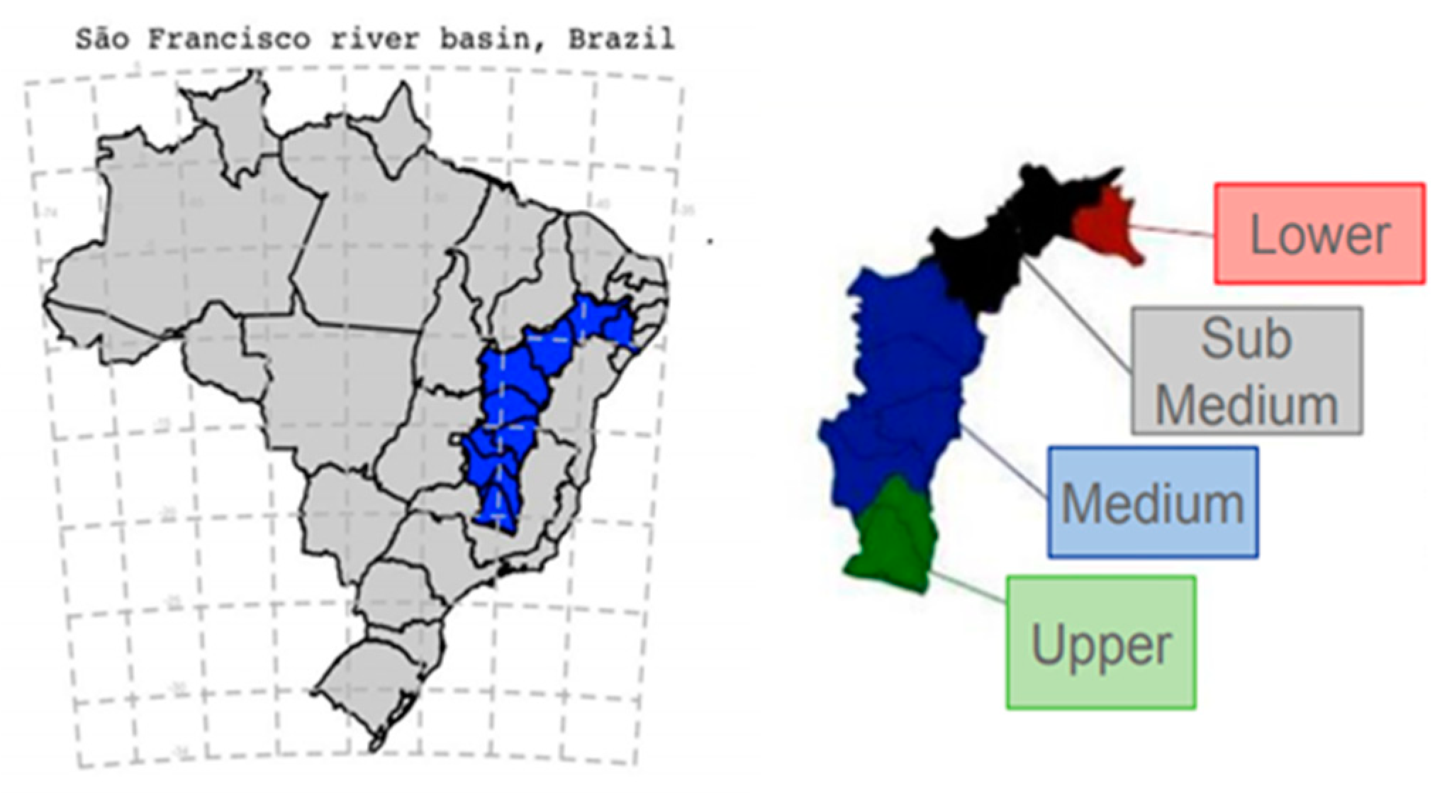
Figure 2.
10-day accumulated precipitation, starting from September 1st, averaged over 2011 and 2015: (a) Eta model simulation (b) CMORPH observed data. The 60-day simulations are discretized in 10 days and referred to as D1, D2, D3, D4, D5, D6.
Figure 2.
10-day accumulated precipitation, starting from September 1st, averaged over 2011 and 2015: (a) Eta model simulation (b) CMORPH observed data. The 60-day simulations are discretized in 10 days and referred to as D1, D2, D3, D4, D5, D6.
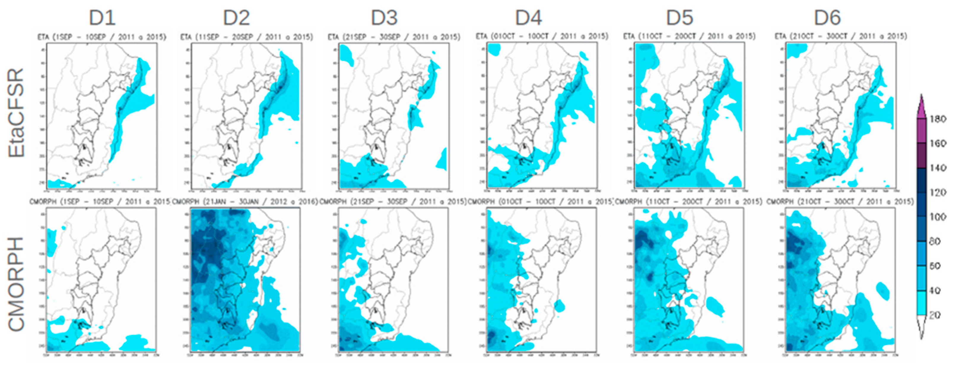
Figure 3.
10-day accumulated precipitation, starting from January 1st, averaged over 2011 and 2015: (a) Eta model simulation (b) CMORPH observed data. The 60-day simulations are discretized in 10 days and referred to as D1, D2, D3, D4, D5, D6.
Figure 3.
10-day accumulated precipitation, starting from January 1st, averaged over 2011 and 2015: (a) Eta model simulation (b) CMORPH observed data. The 60-day simulations are discretized in 10 days and referred to as D1, D2, D3, D4, D5, D6.
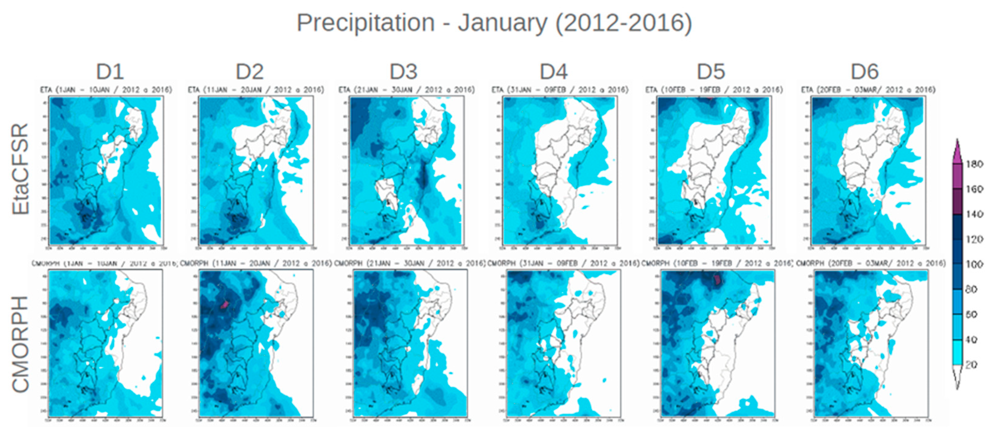
Figure 4.
60-day accumulated precipitation (mm/60 days)starting in September(left) and starting in January( right). The Eta simulations are in solid lines and full dots. The CMORPH data are in dotted lines. Green lines indicate the average rainfall for the Upper SF subbasin, red for the Middle subbasin, blue for the Sub Middle subbasin, and black for the Lower Sao Francisco subbasin.
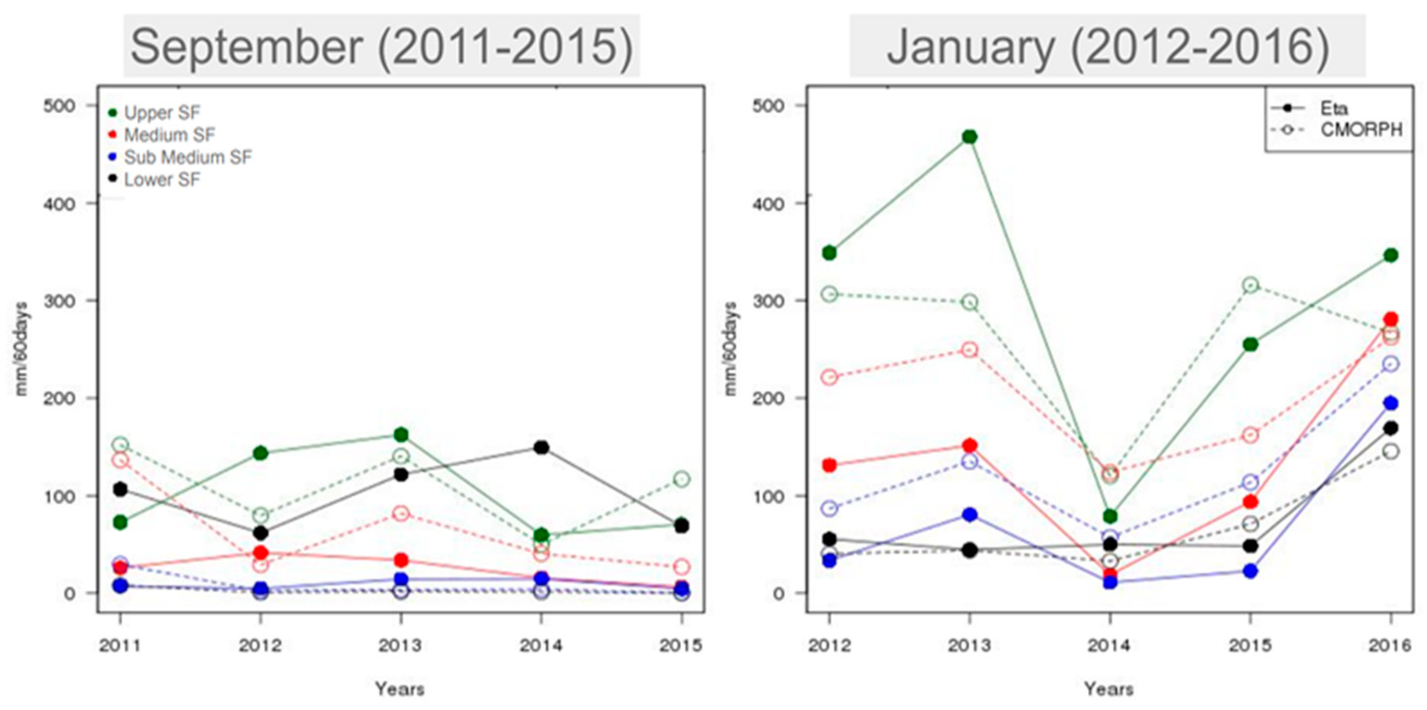
Figure 5.
Boxplot of the 10-day accumulated precipitation (D1, D2, D3, D4, D5, and D6), averaged over 2011-2016, for September and October period, in the different sub-basins of the Sao Francisco River. The Eta simulations are in grey to the left and CMORPH in blue to the right.
Figure 5.
Boxplot of the 10-day accumulated precipitation (D1, D2, D3, D4, D5, and D6), averaged over 2011-2016, for September and October period, in the different sub-basins of the Sao Francisco River. The Eta simulations are in grey to the left and CMORPH in blue to the right.
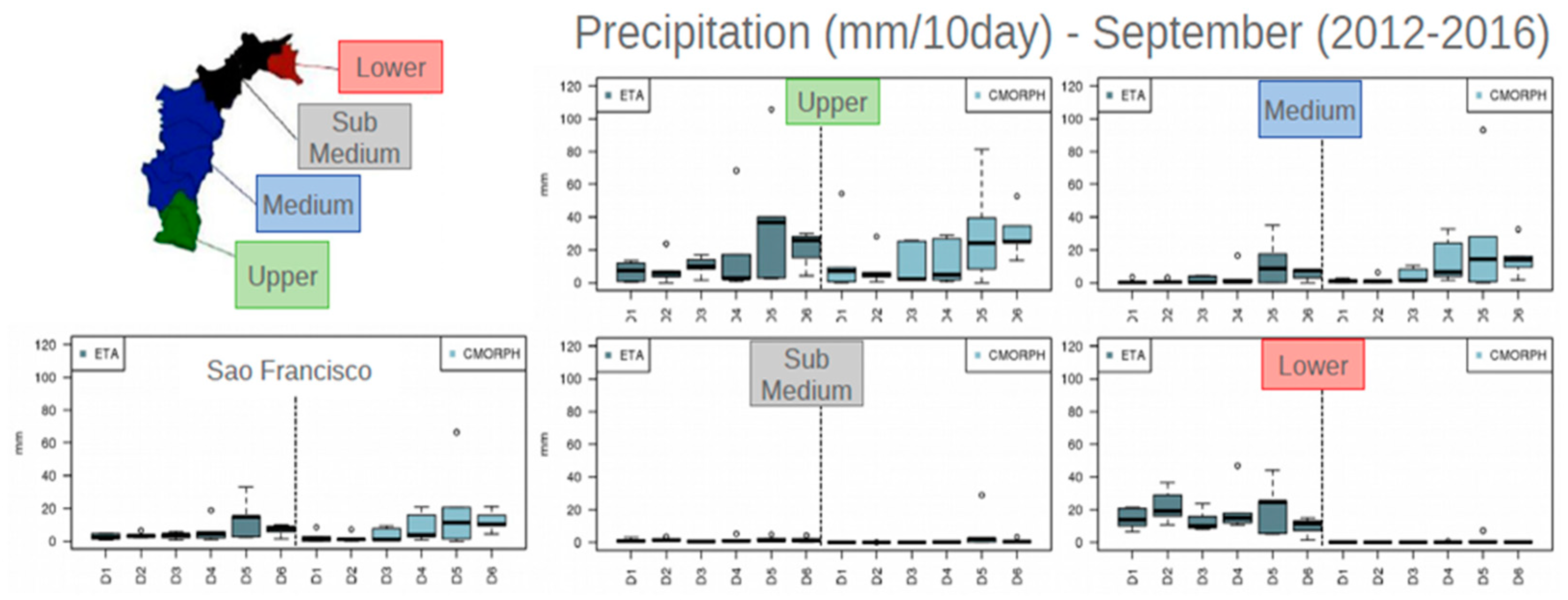
Figure 6.
Boxplot of the 10-day accumulated precipitation (D1, D2, D3, D4, D5, and D6), averaged over 2011-2016, for January and February period, in the different sub-basins of the Sao Francisco River. The Eta simulations are in grey to the left and CMORPH in blue to the right.
Figure 6.
Boxplot of the 10-day accumulated precipitation (D1, D2, D3, D4, D5, and D6), averaged over 2011-2016, for January and February period, in the different sub-basins of the Sao Francisco River. The Eta simulations are in grey to the left and CMORPH in blue to the right.
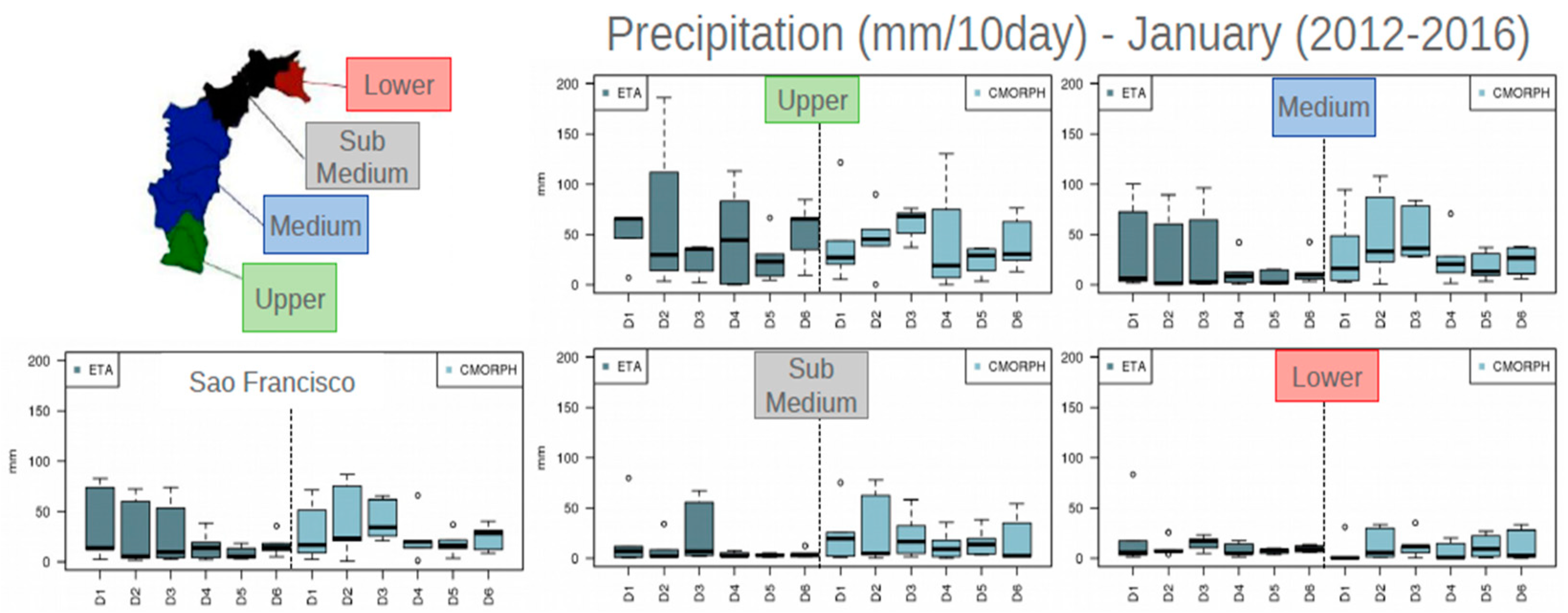
Figure 7.
Linear Correlation between the Eta model simulations and CMORPH precipitation, in each sub-basin of the SF basin and for each 10-day precipitation. Red colors indicate negative correlation and blue colors positive correlation. Correlations are divided into weak (0 to 0.4), moderate (0.4 to 0.7) and strong (0.7 up to 1).
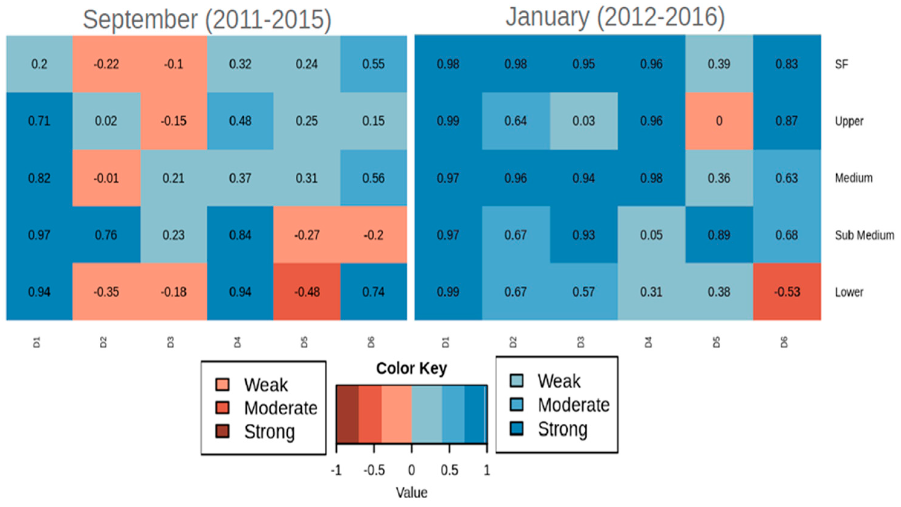
Figure 8.
Mean Absolute Error (MAE) of the Eta model precipitation simulations in each sub-basin of the SF basin and for every 10-day precipitation.
Figure 8.
Mean Absolute Error (MAE) of the Eta model precipitation simulations in each sub-basin of the SF basin and for every 10-day precipitation.
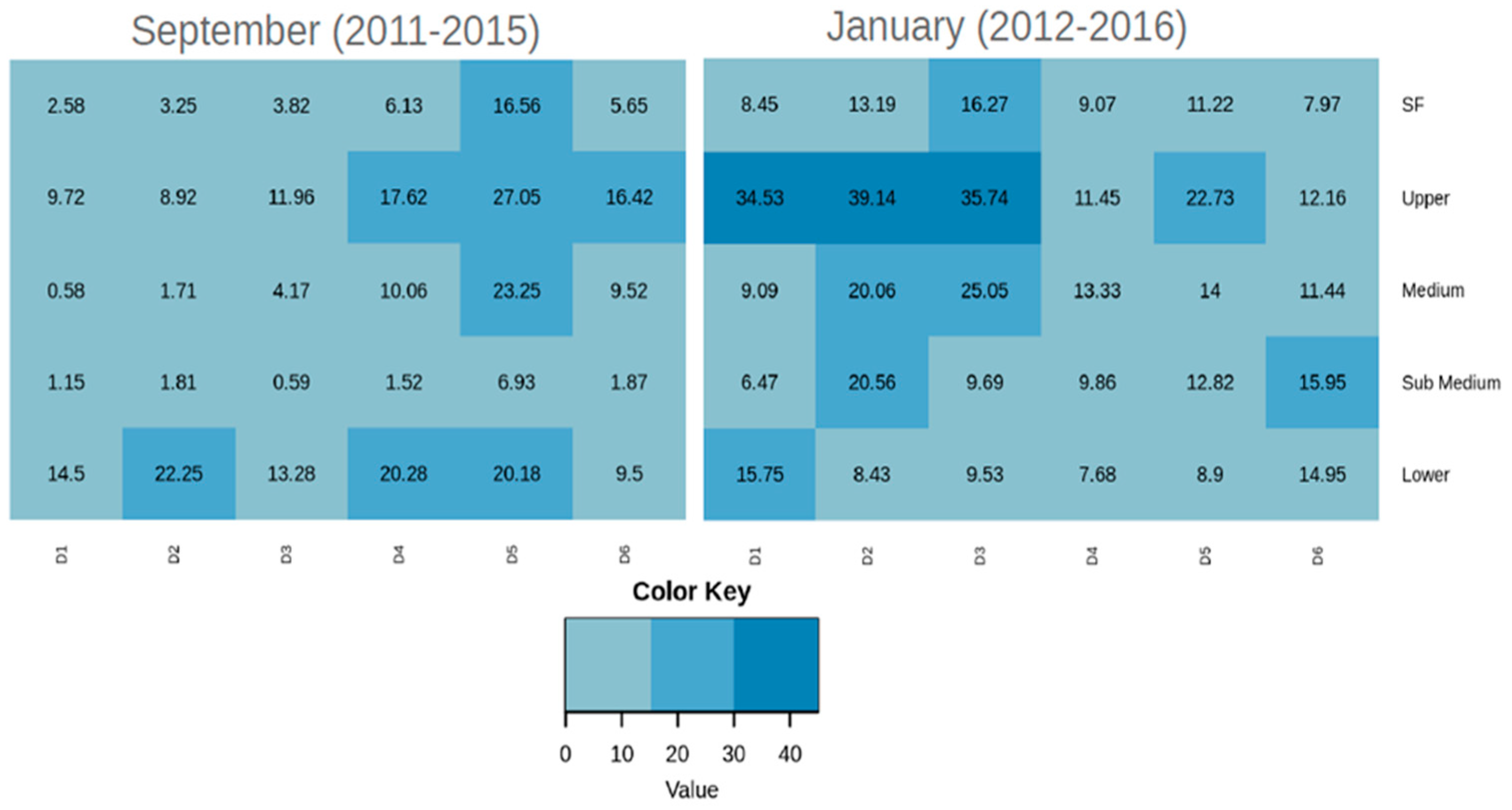
Figure 9.
Mean Error (ME) of the Eta model simulations, in each sub-basin of the Sao Francisco River basin. Red colors indicate negative biases and blue colors positive biases.
Figure 9.
Mean Error (ME) of the Eta model simulations, in each sub-basin of the Sao Francisco River basin. Red colors indicate negative biases and blue colors positive biases.
Disclaimer/Publisher’s Note: The statements, opinions and data contained in all publications are solely those of the individual author(s) and contributor(s) and not of MDPI and/or the editor(s). MDPI and/or the editor(s) disclaim responsibility for any injury to people or property resulting from any ideas, methods, instructions or products referred to in the content. |
© 2023 by the authors. Licensee MDPI, Basel, Switzerland. This article is an open access article distributed under the terms and conditions of the Creative Commons Attribution (CC BY) license (http://creativecommons.org/licenses/by/4.0/).
Copyright: This open access article is published under a Creative Commons CC BY 4.0 license, which permit the free download, distribution, and reuse, provided that the author and preprint are cited in any reuse.


