
Submitted:
07 October 2023
Posted:
10 October 2023
You are already at the latest version
Abstract
The innate immune system is the first line of defense against pathogens. It’s composition includes barriers, mucus and other substances as well as phagocytic and other cells. The purpose of the paper is to analyze in general grounds the immune system and the body immunity to cancer. Simple ideas and the qualitative theory of differential equations are used along with general principles such as the minimization of the pathogen load and economy of resources. In the simplest linear model, the annihilation rate of pathogens in any tissue should be greater than the pathogen’s average rate of growth. When nonlinearities are added, a reference value for the number of pathogens is set, and a stability condition emerges, which relates strength of regular threats, barrier height and annihilation rate. On the other hand, in cancer immunity, the linear model leads to an expression for the lifetime risk, which accounts for both the effects of carcinogens (endogenous or external) and the immune response. The stability condition allows a comparison of immunity in different tissues. The way the tissue responds to an infection shows a correlation with the way it responds to cancer. These statements are formulated at the qualitative level, but may and deserve to be quantitatively checked.
Keywords:
immune system
; dynamics
; infectious process
; cancer
1. Introduction
Human immunity is, as there are practically all physical aspects of life, a control process. Our body senses the number of pathogens in a tissue and a response is generated, which reduces the pathogen load.
The vertebrates immune system has evolved over millions of years to protect the host from infection through a multilayered defense strategy, compressing a variety of sensors, signals and effectors at the cellular level [1]. This includes the innate and adaptive arms of immunity, which work cooperatively to recognize, respond to, and remember pathogens.
The innate immune system, provides rapid first-line protection against infection in a nonspecific manner. Its components include physical and chemical barriers, phagocytic cells (neutrophils, monocytes/macrophages), natural killer (NK) cells, the complement system, and inflammatory signaling molecules called cytokines. Innate immune defenses identify pathogens through pattern recognition receptors (PRRs) [2] that bind conserved molecular patterns on microbes, known as pathogen-associated molecular patterns (PAMPs). Innate immunity is also known to play an important role in antitumor responses by detecting tumors, activating adaptive immunity, and exerting direct effector functions emerging cancer cells [3].
In the present paper, we would like to present a general perspective. Our approach is similar in spirit to systems biology works [4,5], although our view emphasizes on general trends and qualitatively compare the response in different tissues.
The general principles are very simple: first, the pathogen load should be minimized, and second, the used resources should be minimal. These principles should constrain the parameters describing the immune system in any tissue.
2. Results
2.1. Linear model
Let us consider, for example, a very small intensity threat to a given tissue in an adult individual. The resident cells of the immune system will trigger a response to clear the infection. These are, basically, resident cells of the innate system [6]. The simplest available model for the response is a linear one:
in which the response is proportional to the threat. is time, P is the number of pathogens (in some units), and a its rate of growth, typically ∼ 1/hour for bacteria [7]. A freely evolving group of a few streptococci, for example, would lead in around 40 hours to a colony greater than the number of cells in the lungs.
The coefficient , on the other hand, is the tissue annihilation rate of pathogens which, for consistency, should be greater than a in order that small threats do not transform into acute health problems in short terms. This condition requires enough number of resident immune cells in the tissue. This statement may be explicitly formulated and experimentally checked:
Statement 1.
In any tissue, the annihilation rate of pathogens, due to the resident immune cells, is greater than the average multiplication rate of pathogens.
Finally, is the rate of entrance of pathogens into the tissue. The constant will model barrier or mucosal immunity, that is, the flow of pathogens, , is partially trapped and cleared by the barrier or mucosa (or both).
According to Equation (1) , a finite load of pathogens is always annihilated, irrespective of the total number. This unrealistic situation is corrected in nonlinear models, characteristic of self-regulated systems.
2.2. Nonlinear model.
We use a modification of Model 5 of Ref. [8] in order to take account of nonlinearities:
The a parameter equals 0.6 hours. The added nonlinearity limits the increase of P to values below , a conventional parameter indicating sepsis. Authors of paper [8] use an average value of b for the body of 1.5 hours, a value satisfying the requirement , mentioned in the previous paragraph. The parameter limits also the immune response for high values of P.
2.3. Reference value for the number of pathogens.
We draw in Figure 1 the r.h.s. of Equation (2) for and =1.5 hours, which shows two of the fixed points of the equation: (healthy tissue), and , which is an unstable fixed point dividing healthy from septic conditions. If, in the time evolution according to Equation (2), P reaches values greater than , then the final outcome will be a state with P close to . This is the third fixed point of the equation, not seen in the figure.
We can roughly estimate by expanding the r.h.s. of Equation (2) in series of P, retaining linear and quadratic terms, and equating the result to zero, we get:
The last expression comes from neglecting a against . We will assume that there is a unique for all of the tissues. This sets a reference value for in the whole body. could, probably, be associated to the threshold value for initiating recruitment of additional immune cells.
2.4. Stability condition in tissues.
The response coefficient , apart from being greater than a, depends on the pathogen load the tissue is regularly exposed to. If the flow of pathogens, f, is practically constant in certain time intervals, one can get an stability condition by requiring the r.h.s. of Equation (2) to be lower than zero. This leads to:
is the value at the minimum defined in Figure 1. If the inequality is violated, the r.h.s. of Equation (2) is always greater than zero and P increases towards . The estimation for comes from expanding the r.h.s. in series, in the same way as we did for .
Coefficients and shall combine in each tissue in order to guarantee Equation (4) to hold, i.e. guarantee immunity against regular threats. Higher threats would require higher barriers (smaller ) and higher annihilation rates (). This is typical of epithelial tissues. In other cases, for example germinal cells in testis, in order to prevent autoimmunity the coefficient is reduced, which is compensated by high barriers. In summary, we may formulate a second explicit statement,suitable also for experimental verification:
Statement 2.
Minimization ofPleads to the condition (4) for the coefficientsandin terms of the regular pathogen flow in the tissue,. Economy of resources implies that the inequality should be near optimal. There is roughly a similarvalue in all tissues.
2.5. A second consequence of the unstable fixed point.
The unstable fixed point not only sets a unique reference value, , but is also the reason for an interesting property of the small-P response. When the pathogen load overcomes the stability threshold given by Equation (4), the fixed point slows down the increase of P. The reason is very simple: P should traverse the region near , where the r.h.s. of Equation (2) is near zero, that is, where the net annihilation rate of pathogens surpassing the barrier is close to its effective rate of growth. This is shown in Figure 2, where hours and hours. The increase of P is delayed for more than 20 hours, in spite of the fact that the characteristic time scale of the problem is around one hour. This delay allows recruitment of immune cells from blood circulation. We may formulate the following:
Statement 3.
Violation of the stability condition, Equation (4), leads to an impass phase allowing recruitment of other immune cells.
This statement can also be experimentally checked.
2.6. A qualitative comparison.
The following example is a qualitative comparison between two nearby tissues: the small and large intestines. An understanding of the reinforced immunity of the small intestine comes from this analysis.
We show in Figure 3 a schematics of the density of microbes in the contact region. These microbes are mainly commensal bacteria, but it is reasonable to assume that the pathogen loads are proportional to these numbers.
The variable l is a coordinate along the gut. The small bowel is located at , and the large intestine at . The mean value of microbes/gm experiences a jump from to as we cross from the ileum to the cecum [10]. Of course, we expect the dependence to be continuous, as schematically represented in Figure 3.
The parameter values for the large intestine, and , are roughly constant. In the small intestine, however, the parameters shall exhibit a spatial variation. shall decrease and increase as l moves towards the distal end of the ileum. Significant variations of the parameters are expected due to the augmented flow of pathogens in many orders of magnitude. This is consistent with the distribution of Paneth cells [11], Peyer’s patches [12] and other structures along the small bowel. Above, we speak about a “reinforced” immune protection in the small intestine in this sense, the coefficients and shall vary in order to increase protection as increases.
Statement 4.
The distribution of immune structures in the small bowel is related to the increasing density of pathogens observed as we cross from the ileum to the cecum.
2.7. Other tissues.
The stability condition, Equation (4), allows also the analysis of tissues in which the flow of pathogens is normal, but is decreased at the expenses of lowering . These are, for example, the brain [13] and testis [14], where a limit to the cellular immune response is needed for a proper functioning of the tissue. Recall that the values for can never be lower than a, as mentioned.
In addition, there are also tissues, like the gallbladder, where the microbicide character of bile [15] could be translated into a lower than average and, possibly, a low . Notice that we have generalized the meaning of the “barrier” coefficient, , not limited now to anatomical or mucosal barriers.
In conclusion, we assume that the coefficients and take different values for different tissues. The regular flow the tissue is exposed to, , basically determines the ratio , according to Equation (4). The tissue’s functioning conditions could dictate additional restrictions. For example, in the brain should be relatively low in order to avoid frequent inflammation processes, thus should be decreased.
2.8. Immunity to cancer.
Although the detailed dynamics of cancer onset and development is very complex [16], and partially unknown, one may guess that there should be an inverse correlation between the annihilation rate of pathogens in a tissue, , and the risk of cancer. Indeed, the cellular immune response is not only responsible of eliminating virus infected cells, for example, but also dysfunctional and precancerous cells in the tissue. Thus, a low could be related to a higher than normal cancer risk in that tissue. Conversely, one may obtain information for from the frequency distribution of cancer in the body tissues [17].
It is reasonable to assume that, for the initial stages of tumors in a tissue, an equation similar to Equation (1) holds:
where N is the (small) number of precancerous cells, is the rate of creation of such cells in the tissue, is their division rate, and - the tissue’s annihilation rate of dysfunctional cells. can be estimated from the division rate of stem cells in that tissue, , assuming that cancer cells originate from stem cells [18]. Typically, or even smaller [19]. On the other hand, , as noticed. Thus, .
Statement 5.
The tissue annihilation rate of dysfunctional and precancerous cells is similar to the annihilation rate of pathogens.
For , we may use an equation like , where is the number of stem cells, and p - a probability parameter modeling the carcinogenic effect of both internal processes (free radicals, for example) or external factors (double strand breaks by ionizing radiation, for example).
Equating to zero the r.h.s. of Equation (5) and neglecting against , we obtain the average number of precancerous cells in the tissue:
In order to become a true tumor, these cells should pass through a few stages [16], and avoid the adaptive immune system. Nevertheless, it is reasonable to assume that the lifetime risk for cancer in the tissue is proportional to , that is:
where we took years. It is interesting to notice that an expression similar to Equation (7) comes also from a model of oncogenesis in gene expression space [17]. We refer to that paper for a more detailed analysis. For consistency, we reproduce the qualitative inference of () from cancer risk data.
Figure 4 is a re-plot of the results by Tomasetti and Vogelstein [19] (see also [20]) showing the dependence of the lifetime risk for cancer in a tissue on the number of stem cells, and the rate of mitotic divisions. The y-axis in the figure is the normalized risk, i.e. the risk per stem cell. This normalization allows comparison between tissues with high differences in the number of stem cells. The x-axis, on the other hand, counts the number of stem cell generations along lifetime, , a number roughly proportional to the division rate, . The last term accounts for divisions along the clonal expansion phase during tissue formation. The figure shows that, for a single-cell lineage, the larger the higher the normalized risk also.
In Figure 4, a set of 11 cancers shows a near perfect linear correlation: , where the proportionality coefficient may be roughly written as years, and q measures the success rate of precancerous cells: one in ten thousand cells becomes a tumor, for example.
We shall qualify these tissues as “normal”. For all of them, we expect very similar p and , although they may exhibit very different barriers (). Indeed, we expect a very low in the colon and skin, but in blood, for example. The only “special” case in this group is the cerebellum, with a high barrier and a normal (instead of a low) . This means a possibility higher than the cerebrum to clear any infection [21].
External and genetic factors rise the risk (through p) many times, as compared to normal tissues. For example, smoking multiplies the risk for lung cancer by roughly 20 and, in familial adenomatous polyposis patients, the risk for colon cancer is increased by a factor around 100.
There are also tissues like the brain, germ cells, gallbladder, bones and the thyroid where, in addition to genetic or external factors, the relatively high normalized values for the risk lead one suspect unusually low values of . The brain, germ cells and the gallbladder were briefly discussed above. With regard to bones, it is known that immunity relies strongly on defensins [22], possibly with a relatively low number of resident cells. On the other hand, the thyroid is known to have a close cross-talk with the immune system [23]. It’s dysregulation is the cause of immune disorders. One may speculate that a low number of resident cells is needed in order to prevent autoimmunity in the thyroid.
Finally, we have the small intestine with a normalized risk lower than normal, possibly related to a high averaged , a fact consistent with what was discussed above. The results for the estimated coefficients are summarized in Table 1. Although they are only qualitative results, they allow comparison between tissues, and are a first step towards the understanding of Figure 4 for the lifetime risks of cancer in different tissues. We may formulate the following:
Statement 6.
The characteristics of the immune system for a set of tissues are qualitatively described in Table 1. The cancer risk shows an inverse correlation with the cellular immune response against infections.
3. Discussion
In the paper, we show that simple mathematical ideas lead to interesting results when applied to the innate immune system.
In the first step, the linear model described by Equation (1), it is shown that stability of a tissue against small pathogen threats requires . If this condition is not fulfilled, a small threat would, in a few hours, become a serious health problem.
The linear model is modified, Equation (2), in order to consider that neither the number of pathogens nor the response can grow without limits. Healthy () and septic () states appear as fixed points of the nonlinear (self-regulated) equation. In the middle of the way, an additional unstable fixed point, , signals the transition from healthy to septic regimes. We postulate that the value of is common to all tissues. At this step, the stability condition in a tissue is formulated as, Equation (4):
this inequality relates the regular flow of pathogens in the tissue, , with the coefficients and . We may have, for example, a very high long with a very small and a normal , as in the colon. Or a normal , a small and a small , as in the brain.
We notice that the distribution frequency of cancer in tissues provides indications about the strength of , under the assumption that is correlated with the rate of annihilation of precancerous cells. This statement follows from an estimation of the stationary number of precancerous cells in the tissue, which involves both the probabilities of carcinogenic factors and the strength of the immune response. A low , as it is presumably the situation in the gallbladder, for example, would mean a higher than average number of precancerous cells and, thus, a higher than normal cancer risk in this organ. We hope that the model’s simplicity and the qualitative results following from it will motivate immunologists to quantify in more precise terms the immune response in tissues and in the whole body.
Author Contributions
Conceptualization, A.G; methodology, R.H., J.N. and A.G.; software, R.H and J.N; investigation, R.H., J.N. and A.G.; writing—original draft preparation, A.G.; writing—review and editing, R.H., J.N. and A.G.;. All authors have read and agreed to the published version of the manuscript.
Funding
This research received no external funding.
Data Availability Statement
The data for Figure 4 is available in the supplementary materials of Ref. [19]. The code used to generate the figures is available at the GitHub repository: https://github.com/RobertoHePe/F-S-Dynamics.
Acknowledgments
The authors acknowledge the Cuban Agency for Nuclear Energy and Advanced Technologies (AENTA) and the Office of External Activities of the Abdus Salam Centre for Theoretical Physics (ICTP) for support.
Conflicts of Interest
The authors declare no conflict of interest.
References
- Murphy, K.; Weaver, C. Janeway’s immunobiology; Garland science, 2016.
- Akira, S.; Uematsu, S.; Takeuchi, O. Pathogen recognition and innate immunity. Cell 2006, 124, 783–801. [Google Scholar] [CrossRef] [PubMed]
- Demaria, O.; Cornen, S.; Daëron, M.; Morel, Y.; Medzhitov, R.; Vivier, E. Harnessing innate immunity in cancer therapy. Nature 2019, 574, 45–56. [Google Scholar] [CrossRef]
- Mohler, R.R.; Lee, K.S.; Asachenkov, A.L.; Marchuk, G.I. A systems approach to immunology and cancer. IEEE transactions on systems, man, and cybernetics 1994, 24, 632–642. [Google Scholar] [CrossRef]
- Davis, M.M.; Tato, C.M.; Furman, D. Systems immunology: just getting started. Nature immunology 2017, 18, 725–732. [Google Scholar] [CrossRef] [PubMed]
- Davies, L.C.; Jenkins, S.J.; Allen, J.E.; Taylor, P.R. Tissue-resident macrophages. Nature immunology 2013, 14, 986–995. [Google Scholar] [CrossRef] [PubMed]
- Beckers, H.; Van der Hoeven, J. Growth rates of Actinomyces viscosus and Streptococcus mutans during early colonization of tooth surfaces in gnotobiotic rats. Infection and Immunity 1982, 35, 583–587. [Google Scholar] [CrossRef] [PubMed]
- Mai, M.; Wang, K.; Huber, G.; Kirby, M.; Shattuck, M.D.; O’Hern, C.S. Outcome prediction in mathematical models of immune response to infection. PloS one 2015, 10, e0135861. [Google Scholar] [CrossRef] [PubMed]
- Nemytskii, V.V. Qualitative theory of differential equations; Vol. 2083, Princeton University Press, 2015.
- O’Hara, A.M.; Shanahan, F. The gut flora as a forgotten organ. EMBO reports 2006, 7, 688–693. [Google Scholar] [CrossRef] [PubMed]
- Clevers, H.C.; Bevins, C.L. Paneth cells: maestros of the small intestinal crypts. Annual review of physiology 2013, 75, 289–311. [Google Scholar] [CrossRef] [PubMed]
- Jung, C.; Hugot, J.P.; Barreau, F.; others. Peyer’s patches: the immune sensors of the intestine. International journal of inflammation 2010, 2010. [Google Scholar] [CrossRef] [PubMed]
- Van Sorge, N.M.; Doran, K.S. Defense at the border: the blood–brain barrier versus bacterial foreigners. Future microbiology 2012, 7, 383–394. [Google Scholar] [CrossRef] [PubMed]
- França, L.R.; Auharek, S.A.; Hess, R.A.; Dufour, J.M.; Hinton, B.T. Blood-tissue barriers: morphofunctional and immunological aspects of the blood-testis and blood-epididymal barriers. Biology and Regulation of Blood-Tissue Barriers 2013, pp. 237–259.
- Merritt, M.E.; Donaldson, J.R. Effect of bile salts on the DNA and membrane integrity of enteric bacteria. Journal of medical microbiology 2009, 58, 1533–1541. [Google Scholar] [CrossRef] [PubMed]
- Frank, S.A. Dynamics of cancer: incidence, inheritance, and evolution; Princeton University Press, 2007.
- Herrero, R.; Leon, D.A.; Gonzalez, A. A one-dimensional parameter-free model for carcinogenesis in gene expression space. Scientific Reports 2022, 12, 4748. [Google Scholar] [CrossRef] [PubMed]
- Reya, T.; Morrison, S.J.; Clarke, M.F.; Weissman, I.L. Stem cells, cancer, and cancer stem cells. nature 2001, 414, 105–111. [Google Scholar] [CrossRef] [PubMed]
- Tomasetti, C.; Vogelstein, B. Variation in cancer risk among tissues can be explained by the number of stem cell divisions. Science 2015, 347, 78–81. [Google Scholar] [CrossRef] [PubMed]
- Wu, S.; Powers, S.; Zhu, W.; Hannun, Y.A. Substantial contribution of extrinsic risk factors to cancer development. Nature 2016, 529, 43–47. [Google Scholar] [CrossRef] [PubMed]
- Hooper, D.C.; Phares, T.W.; Kean, R.B.; Mikheeva, T. Regional Differences in Blood-Brain Barrier. J Immunol 2006, 176, 7666–7675. [Google Scholar]
- Varoga, D.; Wruck, C.; Tohidnezhad, M.; Brandenburg, L.; Paulsen, F.; Mentlein, R.; Seekamp, A.; Besch, L.; Pufe, T. Osteoblasts participate in the innate immunity of the bone by producing human beta defensin-3. Histochemistry and cell biology 2009, 131, 207–218. [Google Scholar] [CrossRef] [PubMed]
- Perrotta, C.; De Palma, C.; Clementi, E.; Cervia, D. Hormones and immunity in cancer: are thyroid hormones endocrine players in the microglia/glioma cross-talk? Frontiers in Cellular Neuroscience 2015, 9, 236. [Google Scholar] [CrossRef] [PubMed]
Figure 1.
The r.h.s. of Equation (2) for and =1.5 hours. A stable fixed point at , and an unstable one at are signaled. A third, stable one, at , corresponds to a septic state, which is not seen in the figure. The value of the function at the minimum, , is indicated.
Figure 1.
The r.h.s. of Equation (2) for and =1.5 hours. A stable fixed point at , and an unstable one at are signaled. A third, stable one, at , corresponds to a septic state, which is not seen in the figure. The value of the function at the minimum, , is indicated.
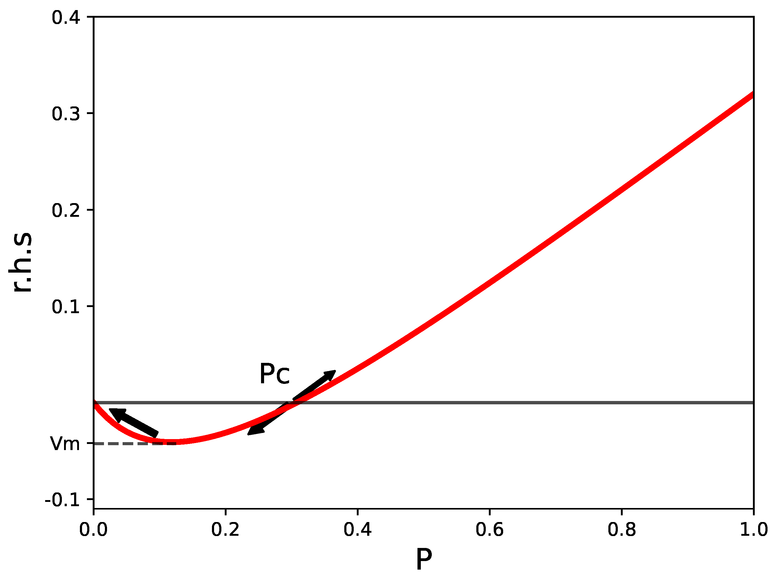
Figure 2.
Time evolution of P according to Equation (2) in the unstable regime hours hours.
Figure 2.
Time evolution of P according to Equation (2) in the unstable regime hours hours.
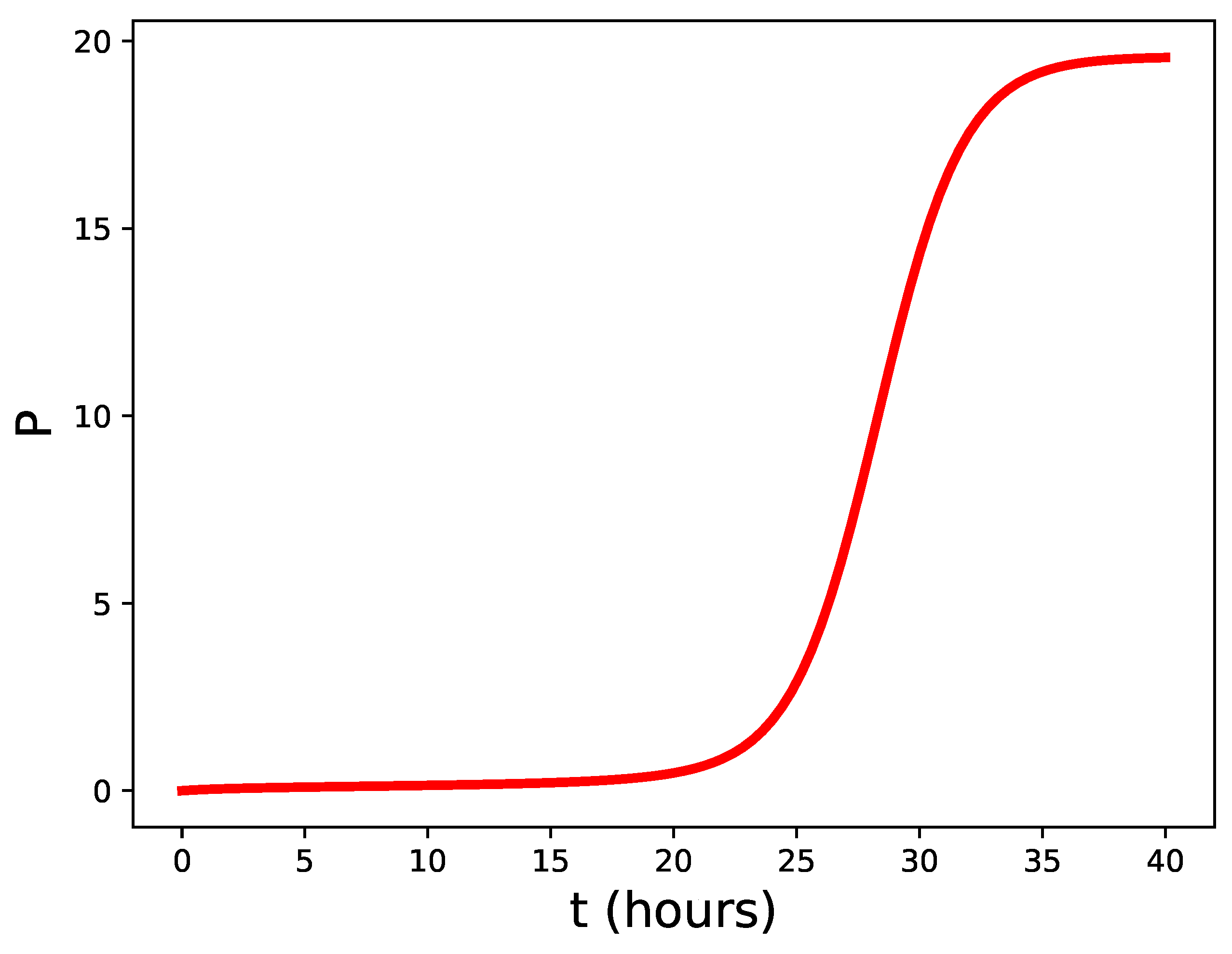
Figure 3.
Schematic representation of the density of microbes in the gut.
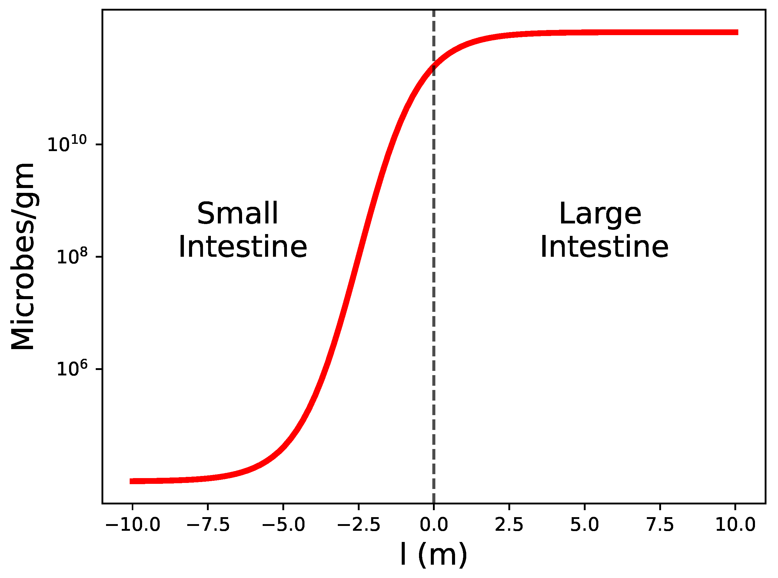
Figure 4.
Lifetime cancer risk in tissues. The figure is a re-plot of the data contained in Tomasetti and Vogelstein paper [19].
Figure 4.
Lifetime cancer risk in tissues. The figure is a re-plot of the data contained in Tomasetti and Vogelstein paper [19].
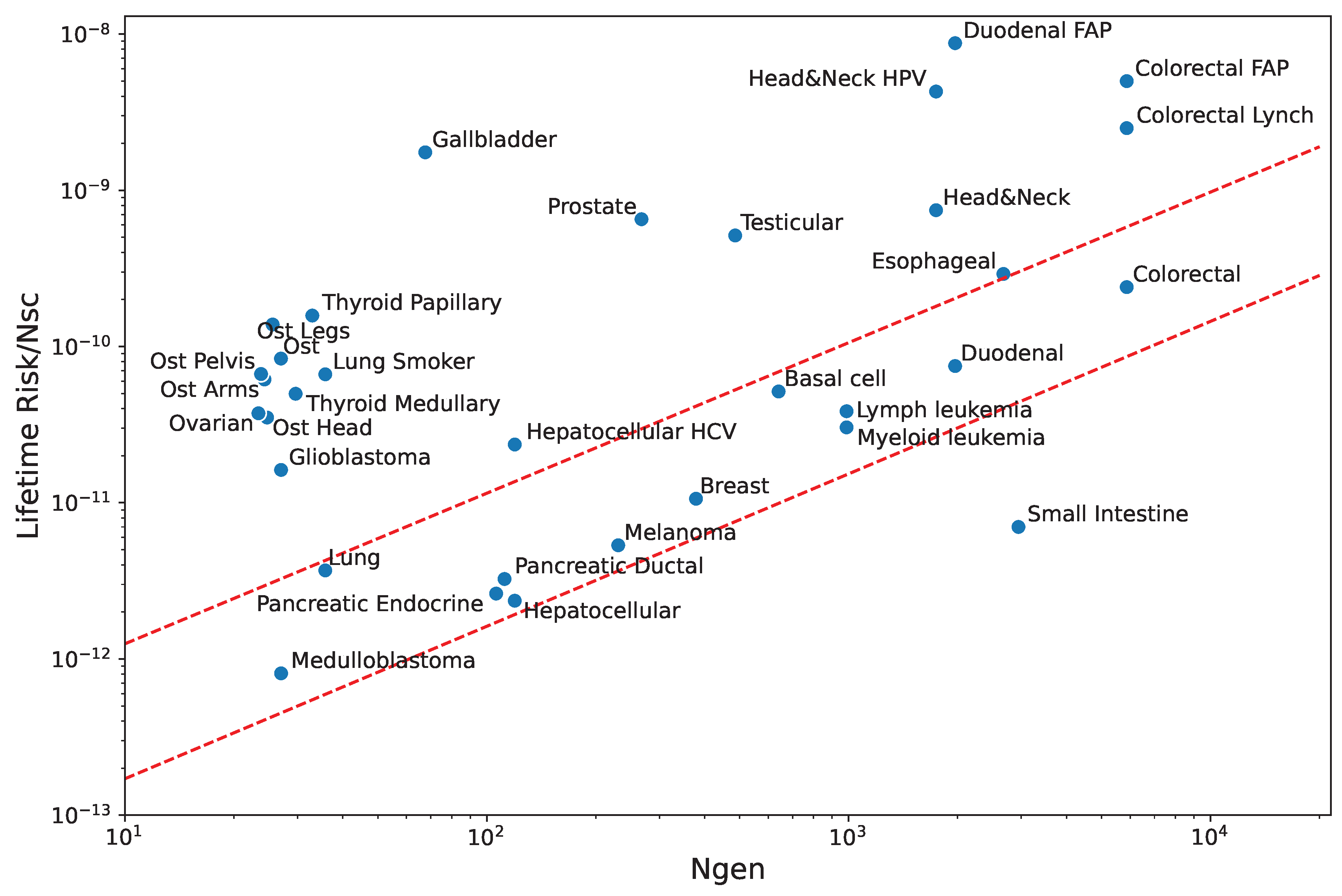

Table 1.
Qualitative comparison of immunity in tissues. The cancer risk per stem cell assumes no external carcinogens or genetic predisposition.
Table 1.
Qualitative comparison of immunity in tissues. The cancer risk per stem cell assumes no external carcinogens or genetic predisposition.
| Tissue | Pathogen | Barrier height | Annihilation | Cancer |
|---|---|---|---|---|
| flow () | () | rate () | risk | |
| Small bowel | Very High | High | High | Low |
| Colon | Very High | Very High | Normal | Normal |
| Lung | Very High | Very High | Normal | Normal |
| Skin | Very High | Very High | Normal | Normal |
| Duodenum | High | High | Normal | Normal |
| Blood | Normal | Normal | Normal | Normal |
| Pancreas | Normal | Normal | Normal | Normal |
| Liver | High | High | Normal | Normal |
| Cerebellum | Normal | High | Normal | Normal |
| Esophagus | High | High | Normal | Normal |
| Head & Neck | Normal | Normal | Normal | Normal |
| Germ cells | Normal | High | Low | High |
| Brain | Normal | High | Low | High |
| Gallbladder | Normal | High | Low | High |
| Bone | Normal | High | Low | High |
| Thyroid | Normal | High | Low | High |
Disclaimer/Publisher’s Note: The statements, opinions and data contained in all publications are solely those of the individual author(s) and contributor(s) and not of MDPI and/or the editor(s). MDPI and/or the editor(s) disclaim responsibility for any injury to people or property resulting from any ideas, methods, instructions or products referred to in the content. |
© 2023 by the authors. Licensee MDPI, Basel, Switzerland. This article is an open access article distributed under the terms and conditions of the Creative Commons Attribution (CC BY) license (http://creativecommons.org/licenses/by/4.0/).
Copyright: This open access article is published under a Creative Commons CC BY 4.0 license, which permit the free download, distribution, and reuse, provided that the author and preprint are cited in any reuse.


