
Submitted:
08 October 2023
Posted:
08 October 2023
You are already at the latest version
Abstract
Process safety plays a vital role in the modern process industry. To prevent undesired accidents caused by malfunctions or other disturbances in complex industrial processes, considerable attention has been paid to data-driven fault detection techniques. To explore the underlying manifold structure, manifold learning methods including Laplacian eigenmaps, locally linear embedding, and Hessian eigenmaps have been utilized in data-driven fault detection. However, only the partial local structure information is extracted from the aforementioned methods. In this paper, these typical manifold learning methods are synthesized to find the underlying manifold structure from different angles. A more comprehensive local structure is discovered under a unified framework by constructing an objection optimization function for dimension reduction of the process data. The proposed method takes advantage of different manifold learning methods. Based on the proposed dimension reduction method, a new data-driven fault detection method is developed. Hotelling’s T2 and Q statistics are established for the purpose of fault detection. Experiments on an industrial benchmark Tennessee Eastman process and a real blast furnace ironmaking process are carried out to demonstrate the superiority and effectiveness of the proposed method.
Keywords:
Data-driven method
; Fault detection
; Manifold Learning
; Blast Furnace Ironmaking Process
1. Introduction
Industrial processes are becoming more complex and their hazards to the environment are receiving increasing attention. Process safety is a non-negligible component of industrial processes, which comprises several steps such as hazard identification and analysis [1]. In particular, the identification and analysis of hazards is a key step in the prevention and mitigation of major process accidents.
In industrial processes, timely and accurately identifying abnormal operating conditions can prevent major accidents and improve operational efficiency, thus achieving compliance with environmental and safety regulations. Dynamic process monitoring for hazard/fault identification is already a trend in the future development of process safety and risk management [2]. Real-time monitoring of process operations to ensure safety measures is an essential step in the modern process industry [3].
Fault detection plays a pivotal role in guaranteeing operation safety and reducing downtime in complex industrial processes [4,5]. Broadly speaking, fault detection techniques can be categorized into three classes, model-based, knowledge-based, and data-driven based methods [6]. Model-based methods rely on the mathematical model. However, the mathematical model is often difficult or time-consuming to establish for complex industrial processes such as the blast furnace ironmaking process. For knowledge-based methods, the model is built from expert knowledge or qualitative information, which limits its applications for complex industrial processes. Conversely, only the measured process variables are required for data-driven fault detection methods. Thus, data-driven techniques are more suitable and efficient for the fault detection of complex industrial processes [7]. With the advance of the sensor, communication, and computing technologies, large amounts of data are collected in modern industrial processes. Under such circumstances, data-driven fault detection has gained an explosive amount of attention in recent years both from academia and industry [8].
To handle the highly correlated high-dimensional process data, multivariate analysis (MVA) has been widely employed in industrial processes [9]. In MVA, the process behavior is modeled by transforming the high-dimensional data into a lower-dimensional space. The features are extracted for establishing monitoring statistics. Among the MVA based fault detection methods, principal component analysis (PCA) has gained widespread popularity in process monitoring and fault diagnosis in the past decades [10]. In PCA, process data is projected into a lower-dimensional space to preserve the significant variability information as much as possible. Due to its efficiency and simplicity, PCA has been successfully applied in a large number of industrial processes [11]. Despite this, PCA is regarded as a kind of globality-based linear dimensionality reduction technique. However, the process data mostly lie on or close to a low-dimensional manifold. Compared to globality-based methods, manifold learning is an approach to nonlinear dimensionality reduction through discovering the manifold structure of data. In manifold learning, the input data is assumed to be sampled from a low-dimensional manifold. Representative manifold learning methods include Isomap [12], Locally Linear Embedding (LLE) [13], Laplacian eigenmaps (LE) [14], Local Tangent Space Alignment (LTSA) [15], Locality Preserving Projections (LPP) [16], Neighborhood preserving embedding (NPE) [17], and Hessian eigenmaps (or called Hessian LLE) [18].
In NPE, each data point is represented as a linear combination of the neighboring data points. Then, an optimal embedding is found to preserve the neighborhood structure in the dimensionality reduced space [17]. Chen et al. [19] applied eigenvalue decomposition and generalized eigenvalue decomposition to solve the unstable problem caused by singularity problem in NPE, and developed an NPE-based incipient fault detection method for small-scale cyber-physical systems. Since the NPE method can preserve the local manifold structure of different modes, Song et al. [20] performed NPE on the time-lagged variables for multimode dynamic process monitoring. LPP is designed to find the optimal linear approximations to the eigenfunctions of the Laplace Beltrami operator on the manifold through the nearest neighbor search in the low-dimensional space [16]. Duan et al. [21] employed LPP to preserve the local structure of process data, then adopted least squares support vector machine to predict the key-performance-indicator. Zhang et al. [22] combined LPP and PCA to preserve both global and local structures of the data set and developed fault detection and identification method by utilizing the extracted features. LLE attempts to discover nonlinear structure in high-dimensional data by exploiting the local symmetries of linear reconstructions [18]. Wu et al. learned structure information by LLE and incorporated the extracted local information into canonical correlation analysis (CCA) for quality-relevant nonlinear process monitoring [23]. Li and Zhang implemented the supervised locally linear embedding projection method for bearing fault diagnosis and illustrated its validity using the experimental data [24]. Different manifold learning methods focus on uncovering the manifold structure with different criteria. It relies on the knowledge and experience of experts for their own purposes. Therefore, only partial information from the underlying manifold is learned by each existing local manifold learning method. To take advantages of different manifold learning methods for better discovering the underlying manifold structure, Xing et al. [25] provided a common framework to synthesize the partial information extracted from different local manifold learning methods under local tangent coordinates.
Motivated by the above discussions, a novel data-driven fault detection based on fused local manifold learning (FLML) is proposed in this paper. In the proposed FLML, the partial information on the geometric structure of the underlying manifold is firstly extracted from LE, LLE, and Hessian Locally Linear Embedding (HLLE) methods, respectively. A novel objective function is formulated to fuse the extracted partial information. On the basis of the optimization results, FLML can learn the geometric information from different local methods. The geometric structure of the underlying manifold is more thoroughly explored by the proposed FLML, compared to LE, LLE, and HLLE. Like the PCA-based fault detection method, two monitoring statistics including Hotelling’s and Q statistics are established. The effectiveness and advantages of the proposed FLML-based fault detection are illustrated by an industrial Tennessee Eastman process benchmark and a real blast furnace ironmaking process.
The rest of this paper is organized as follows. Section II briefly introduces the ideas of LE, LLE, and HLLE. Section III illustrates the proposed FLML method and its application in fault detection in detail. In Section IV, the proposed FLML-based fault detection approach is verified through an industrial Tennessee Eastman (TE) process benchmark and a real blast furnace ironmaking process. Finally, Section V provides the conclusion.
2. Brief Review of LE, LLE and HLLE
2.1. LE
LE is a well-known manifold learning method to extract local structure features in the original sample space. The main idea behind LE is that the corresponding projections of neighboring points in the low-dimensional space should be close if the neighboring points in the high-dimensional space are close [14].
Given a set of n sample points in , where D is the number of variables. The goal of LE is to find a set of points () in the low-dimensional space to have the neighbor relations between sample points in the high-dimensional space.
In LE, the first step is to construct the adjacency graph. k-nearest neighbors () is a widely used neighbors selection strategy, due to its simplicity. To model the neighborhood relations between sample points, an adjacency matrix is employed, where each element represents the neighborhood relations between and its neighbor . Using the Gaussian heat kernel, the adjacency matrix can be formed as follows,
where is the kernel width.
The objective function of LE can be cast as,
where is a diagonal matrix, and is defined as a Laplacian matrix.
The optimization problem (2) is equivalent to generalized eigenvalue problem,
It can be readily solved through eigenvalue decomposition.
2.2. LLE
In LLE, the key assumption is that each data point and its neighbors are lied on or closed to a locally linear patch. A sample can be represented as the linear combination of multiple samples from its neighborhood [13]. The optimization problem of LLE can be formulated as,
where is the weight coefficient and only when and are neighbors the corresponding has a value, otherwise it is 0. Similarly, the neighbors selection can be determined by method.
Denoted the low-dimensional features as , the minimization problem (4) can be formulated as,
where is the identity matrix, is the weight coefficient matrix and .
Similarly, the optimization problem (5) can be solved through eigenvalue decomposition.
2.3. HLLE
HLLE is regarded as a variant of LLE. Assumed that the low-dimensional data representation is locally isometric to an open and connected subset, the idea behind HLLE is to minimize the curviness of the high-dimensional manifold while embedding it into a low-dimensional space [18].
Assumed that the set is located on a smooth manifold with an intrinsic dimension , PCA is firstly performed on to obtain d eigenvectors .
It is assumed that the number of neighbors of the sample is k. Then, the local tangent coordinate of the sample can be calculated by projecting the local neighborhood into the tangent subspace,
Then, the Hessian matrix containing local information will be calculated by the projection of neighbors in the tangent coordinate . Through defining constructing by the [26], can be constructed by the last where is the pseudo-inverse symbol. Therefore, the local objective of HLLE can be estimated with,
where is the local projection and is the smooth function used to estimate the local neighborhood information at a fixed point . Then, extending the local neighborhood information to the all samples, we can get the global projection . The optimization objective of HLLE can be rewritten as,
where is the local objective and the neighboring selection matrix can convert local projection to global projection and each entry of can be obtained as,
For solving the above optimization problem (8), eigenvalue decomposition is also utilized. Details of HLLE can be found in [18].
3. Proposed Method
3.1. FLML: Fused Local Manifold Learning
From the previous section, it can be found that LE, LLE, and HLLE can explore the local geometric structure information from different perspectives. To synthesize these local information, Xing et al. [25] fused the local information obtained by multiple manifold learning methods including LE, LLE, HLLE and LTSA by reformulating the different local manifold algorithms under the local tangent coordinate system to reveal the underlying manifold of the dataset. Similar to [25], the fused local objective is defined as
to integrate LE, LLE, and HLLE. Here, are the fusion coefficients.
Remark 1. In [25], the local objectives are optimized to determine the fusion coefficients and global embedding coordinates simultaneously. In [27], the selection of c is determined by employing the alternating optimization method which iterative updates c and in an alternating fashion. For simplicity, only the global embedding coordinates are obtained in this study. The fusion coefficients are considered fixed values.
Similar to LE, LLE, and HLLE, the proposed FLML method is a kind of linear projection method. To facilitate the online fault detection, an explicit linear mapping from the original space to the low-dimensional space is provided. Thus, the main goal of FLML is to seek a transformation matrix that maps the high-dimensional data to low-dimensional data. Supposed that is the transformation vector from to , therefore, the projections in the low-dimensional space can be represented as .
To synthesize the local geometric structure information and impose constraints to prevent multiple solutions, the objective function of FLML is formulated as follows,
Remark 2. As shown in (10) and (11), it is noticed that the corresponding local structure will be extracted from LE, LLE and HLLE while and are selected to be , and , respectively.
To solve the optimization problem (11), we use the technique of Lagrange multipliers as follows,
where is the Lagrange multiplier.
While , it results in
Hence, we can use generalized eigenvalue decomposition to obtain the transformation vector from (13). Finally, the transformation matrix can be assembled by the eigenvectors corresponding to the smallest d eigenvalues derived from the result of generalized eigenvalue decomposition.
3.2. FLML based Fault Detection
Generally, data-driven fault detection methods contain two steps, offline modeling and online monitoring. In the offline modeling step, the process data are collected under normal operating condition for training. Using the training data , an FLML model is established. Subsequently, the low-dimensional data is obtained. With the transformation matrix , the relation between and can be represented,
The residual matrix is,
In the online monitoring step, the low-dimensional data point and residual of a new standardized sample is obtained,
The Hotelling’s and squared prediction error (SPE) statistics (also called Q statistic) are often used for monitoring. For statistic, the Mahalanobis distance is used to evaluate the variations of . The Hotelling’s statistic is defined as,
where is the covariance matrix of which is extracted from the normal operating condition data .
For Q statistic, the Euclidean distance is adopted to evaluate the magnitude of vector in the residual space as follows,
Under the assumption that all operating parameters and prediction errors have a Gaussian distribution, the upper control limits (UCLs) of Hotelling’s and Q statistics are determined by means of F distribution and distribution, respectively. Thus, with a level of significance , the UCLs are calculated as follows,
where and , is the sample mean and is the sample variance of the statistic Q. g and h are calculated using normal operating condition data.
In FLML, the parameters such as the number of the neighbors k, the bandwidth of Gaussian heat kernel, the fusion weights and , and the number of latent variables d are determined as follows,
- k: The finding of neighborhood relation is related to the selection of k [23]. To balance the computation complexity and generalization capability, we choose k in the range with the smallest mean false alarm rate (FAR). The definition of FAR can be found in next section.
- : If the bandwidth of the Gaussian heat kernel function is too small, the kernel will be sensitive to noise. A large bandwidth may create an overly smooth mapping [28]. Empirically, the bandwidth is chosen as where m is the size of variables, b is a constant, and represents the variance of the data, which is 1 as the original data is normalized [22]. In the case studies, are selected.
- and : It is noticeable that the hyper-parameters and have a important influence on the performance of the proposed FLML method. However, it is a challenging work to choose a set of optimal hyper-parameters. As a traditional way of performing hyper-parameter optimization, the grid search method is employed. For this purpose, a finite set of and are explored by minimizing the mean FAR.
- d: Similar to NPE-based and LPP-based methods, the number of latent variables d is selected by searching for eigenvalues similar to the smallest non-zero eigenvalue.
In summary, the procedure of the FLML based fault detection is described as follows,
Offline training:
Online monitoring:
4. Case Studies
In this section, the proposed FLML-based fault detection method is verified by conducting experiments on the Tennessee Eastman process and a real-world blast furnace ironmaking process.
4.1. Tennessee Eastman Process
The TE process is a well-known and widely used industrial benchmark for comparing the performance of process monitoring and control [29]. In the TE process, there are five main units including a separator, a compressor, a reactor, a vapour/liquid separator, a stripper and a condenser, and eight components A-H. It also has 12 manipulated variables (XMV1-11) and 41 measured variables (XMEAS1-41). Among these variables, XMEAS(23-41) are the composition of A-H measured with 6 min sampling intervals in different positions. Other variables are collected with 3 min sampling intervals. There are 21 preprogrammed faults in TE process. Of 21 faults, due to the absence of observable change in the mean and standard deviation between their corresponding faulty and normal operation, faults 3, 9 and 15 are very difficult to detect [30]. In this study, faults 3,9 and 15 are ignored. The descriptions of the faults considered in this study are listed in Table 1.
A widely used dataset of TE process can be found in http://web.mit.edu/braatzgroup/links.html. In this study, we also adopt this dataset. Specifically, 22 measured variables XMEAS(1:22) and 11 manipulated variables XMV(1:11) are selected as . 500 samples collected under the normal operating condition (IDV(0)) are used as a training dataset. For each faulty dataset, it has 960 samples in total where the fault is injected from the 160th sample.
To assess the fault detection performance, three indices including Missed detection rate (MDR), Detection delay (DD) and false detection rate (FAR) are used. DD is defined as the time interval from the start of fault to the detection time, which is expressed as the first time of 5 consecutive rises. MDR and FAR with a confidence level can be calculated as follows,
where and .
For comparative study, several typical fault detection methods including PCA, NPE, LPP, Principal Component Pursuit (PCP)[31], kernel PCA (KPCA)[32], mixed KPCA (MKPCA) and structured joint sparse PCA (SJSPCA)[33] are employed. For PCA, is set according to the cumulative percentage of variance (CPV). For the NPE, and is selected. For LPP, , , and are selected. For PCP, is selected. For KPCA, the kernel width and is selected. For MKPCA, the kernel widths , are set as 500 and 1000 respectively, and is selected. For SJSPCA, , , , and are selected. As displayed in Figure 1, is selected for the TE case. Similarly, As shown in Figure 2, and are chosen. For FLML, , , , and are selected.
Table 2 and Table 3 list the MDRs and FARs of 18 faults. It can be observed that the NPE and LPP can provide superior performance over PCA. The utilization of local structure information can enhance fault detection performance. On the other hand, FLML statistic offers the lowest MDRs among all the comparative methods. The average of MDRs of FLML statistic is . Compared to NPE and LPP methods, the average of MDRs of FLML statistic is increasingly reduced. Furthermore, the FARs of FLML statistic reach the same level of NPE and LPP. The average of FARs of FLML statistic is . The DD index represents the sensitivity of monitoring statistics. A smaller DD means the monitoring statistic can detect the fault earlier. Table 4 lists the DDs for all methods, where the DD is indicated in the unit of the hour. As displayed in Table 4, FLML statistic can derive the smallest DD among the all methods.
To further illustrate the superiority of the proposed FLML method, the monitoring results are depicted in Figure 3 and Figure 4 by PCA, NPE, LPP, PCP, KPCA, MKPCA, SJSPCA, and FLML methods for IDV (10) and IDV (19), respectively. Fault 10 is designed by adding a random disturbance on the C feed temperature (Stream 4). Compared to the step type fault scenarios such as fault 1, fault 2, fault 10 is more difficult to detect. As shown in Figure 3, it is observed that FLML can detect most of the faulty samples. In contrast, other monitoring statistics such as PCA , NPE , PCP , KPCA , MKPCA , SJSPCA , and LPP can not effectively detect the fault 10, since most of the monitoring statistics are below the corresponding UCLs. Fault 19 is an unknown faulty type. The monitoring results of fault 19 is displayed in Figure 4. By comparison, it can be observed that PCA, NPE, LPP, PCP, KPCA, MKPCA, and SJSPCA fail to detect the occurrence of fault 19. The online statistics are almost lower than the UCLs after 161th sample. A promising result can be obtained using FLML as shown in Figure 4(h).
4.2. Blast Furnace Ironmaking Process
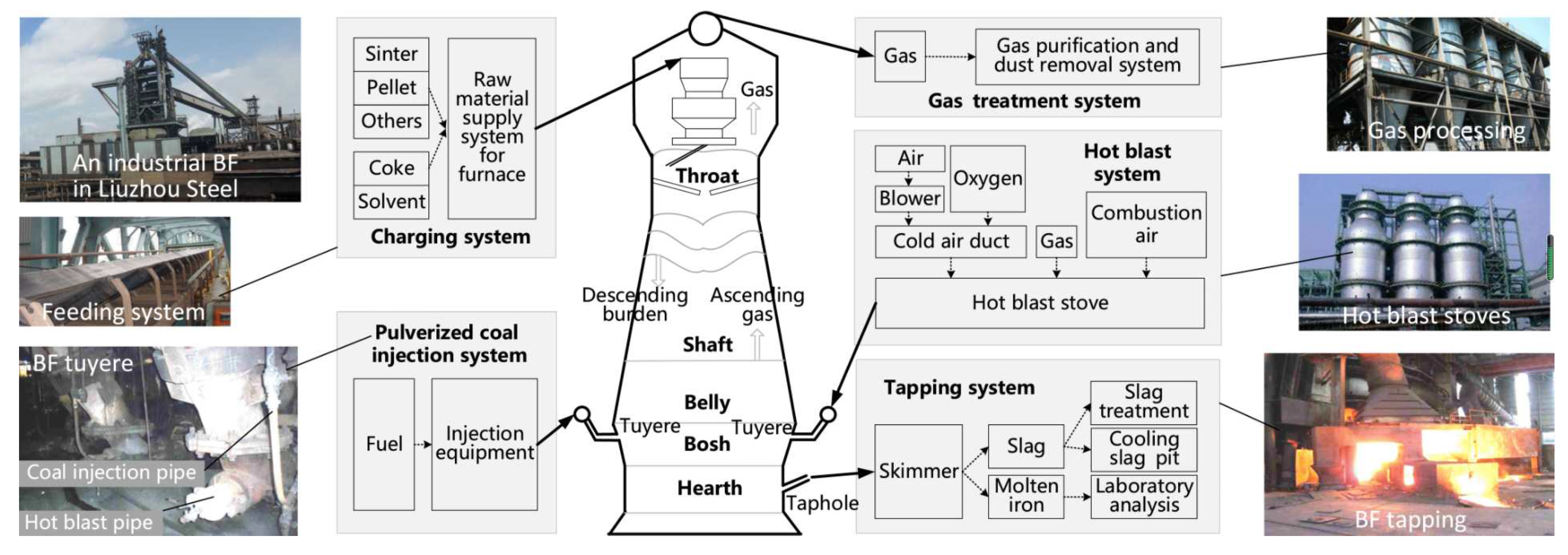
In this section, the proposed method is verified through a real blast furnace (BF) ironmaking process at a steel company in South China. In the steel manufacturing process, the blast furnace ironmaking process plays a vital role. The blast furnace ironmaking process is considered one of the most complex industrial processes. The basic units of the blast furnace ironmaking process are depicted in Figure 5. As it can be seen from Figure 5, the ironmaking process can be mainly divided into several sub-systems including the charging system, gas processing system, hot air system, the pulverized coal injection system, the iron system, and the BF body. The inner structure of the blast furnace is vertical. In the BF, the iron ore and coke are fed from the top along the vertical direction. The hot air and coal powder are blown into the furnace from the bottom. Through complex chemical reactions, the molten iron and slag are generated and accumulated in the hearth. In a periodical way, the molten iron and slag are discharged from the bottom of the furnace through the tap hole. As a byproduct, the flux gas escapes from the top of the furnace.
In the ironmaking process, it often suffers from abnormal furnace conditions, due to the effects of unreasonable daily operation and various disturbances. If these abnormal furnace conditions are not timely detected, the product quality will be degraded, and even the safety of the plant would not be ensured. Thus, the effective detection of abnormalities becomes an indispensable component of the operation of a blast furnace. In this study, we consider the detection of the channeling fault. The channeling fault may be caused by several reasons such as the low-quality coke pulverized coal, the inappropriate adjustment of air volume. In a channeling accident, the high-temperature furnace gas passes in the path of least resistance at a high velocity. The furnace gas increases the heat load at the wall and top of the furnace, resulting in possible equipment damage such as burning of the bag dust catcher [34].
Figure 5.
Diagram of Blast Furnace Ironmaking Process [35].
Figure 5.
Diagram of Blast Furnace Ironmaking Process [35].
In this case, a data set was collected from 2013 12/21 to 2014 01/05. The sampling interval is 10s. As demonstrated in [36], we select 7 variables that are the most sensitive to faults. These variables are listed in Table 5. A total of 1000 samples are collected from 12/21 00:20 to 20-12/28 09:40 under the normal operating conditions as the training dataset. According to the accident report of the operation personnel, from 2013 12/30 23: 44 to 2013 12/31 05: 18, the ironworks accident report has recorded the occurrence of the channeling. To facilitate the verification of fault detection performance, a testing dataset are generated, where 1200 samples were collected where the fault occurred from the 200th sample.
For PCA, is selected. For NPE, the neighbor parameter k and number of principle components d are selected to be 5 and 3, respectively. For LPP, , and are determined. For PCP, is selected. For KPCA, and . For MKPCA, , and . For SJSPCA, , , , and . For fair comparison, , , are selected for FLML. The result of grid search for selecting and is plotted in Figure 6. On the basis of grid search results, and are determined.
The monitoring results are plotted in Figure 7. It can be observed that NPE and LPP statistics can detect more faulty samples than PCA statistic. But, the improvement is limited as shown in Figure 7. The reason may be that NPE and LPP only extract partial local structure information. It is also noticed that there are more false alarms for PCA Q and PCP Q statistics. Compared to the other methods, the proposed FLML method can provide much better performance as shown in Figure 7(h). Only a few faulty samples are missed. Table 6 lists the MDRs, FARs, and DDs. As shown in Table 6, the MDR and FAR of FLML are and , respectively. The DD of FLML is mins. The channeling condition can be timely and accurately detected by FLML . Among these comparative methods, the proposed FLML method can offer the best monitoring performance.
5. Conclusions
In this paper, a novel data-driven fault detection technique based on fusing local manifold learning methods is proposed for complex industrial processes. The proposed method aims to explore a more comprehensive local structure by synthesizing partial information learned from LE, LLE, and HLLE. With the exploit of local geometric structure, the process data is projected into a lower-dimensional space. Hotelling’s and Q statistics are employed for fault detection. Case studies on the widely used TE process benchmark and a real blast furnace ironmaking process show the superior monitoring performance of the proposed methods, by comparison with other related methods. Future work will investigate the application of the proposed method on fault identification and classification.
Author Contributions
Conceptualization, P.W.; Methodology, P.W., K.W.; Investigation P.W.; Writing– original draft, P.W., K.W. and S.L.; Writing – review & editing, P.W., H.P, J.G.; Data Curation, K.W. and J.G.
Acknowledgments
This work was supported in part by the Zhejiang Province Public Welfare Technology Application Research Project (Grant No.LGF19F030004, LGG21F030015), and Open Research Project of the State Key Laboratory of Industrial Control Technology, Zhejiang University, China (No. ICT2023B19).
References
- Bahr, N.J. System safety engineering and risk assessment: a practical approach; CRC press, 2014. [Google Scholar]
- Khan, F.; Rathnayaka, S.; Ahmed, S. Methods and models in process safety and risk management: Past, present and future. Process safety and environmental protection 2015, 98, 116–147. [Google Scholar] [CrossRef]
- Nan, C.; Khan, F.; Iqbal, M.T. Real-time fault diagnosis using knowledge-based expert system. Process safety and environmental protection 2008, 86, 55–71. [Google Scholar] [CrossRef]
- Venkatasubramanian, V.; Rengaswamy, R.; Yin, K.; Kavuri, S.N. A review of process fault detection and diagnosis: Part I: Quantitative model-based methods. Computers & chemical engineering 2003, 27, 293–311. [Google Scholar] [CrossRef]
- Tidriri, K.; Chatti, N.; Verron, S.; Tiplica, T. Bridging data-driven and model-based approaches for process fault diagnosis and health monitoring: A review of researches and future challenges. Annual Reviews in Control 2016, 42, 63–81. [Google Scholar] [CrossRef]
- Dai, X.; Gao, Z. From model, signal to knowledge: A data-driven perspective of fault detection and diagnosis. IEEE Transactions on Industrial Informatics 2013, 9, 2226–2238. [Google Scholar] [CrossRef]
- Yin, S.; Ding, S.X.; Xie, X.; Luo, H. A review on basic data-driven approaches for industrial process monitoring. IEEE Transactions on Industrial Electronics 2014, 61, 6418–6428. [Google Scholar] [CrossRef]
- Qin, S.J.; Chiang, L.H. Advances and opportunities in machine learning for process data analytics. Computers & Chemical Engineering 2019, 126, 465–473. [Google Scholar] [CrossRef]
- Yin, S.; Ding, S.X.; Haghani, A.; Hao, H.; Zhang, P. A comparison study of basic data-driven fault diagnosis and process monitoring methods on the benchmark Tennessee Eastman process. Journal of process control 2012, 22, 1567–1581. [Google Scholar] [CrossRef]
- Dong, Y.; Qin, S.J. A novel dynamic PCA algorithm for dynamic data modeling and process monitoring. Journal of Process Control 2018, 67, 1–11. [Google Scholar] [CrossRef]
- Yin, S.; Li, X.; Gao, H.; Kaynak, O. Data-based techniques focused on modern industry: An overview. IEEE Transactions on Industrial Electronics 2014, 62, 657–667. [Google Scholar] [CrossRef]
- Tenenbaum, J.B.; De Silva, V.; Langford, J.C. A global geometric framework for nonlinear dimensionality reduction. science 2000, 290, 2319–2323. [Google Scholar] [CrossRef] [PubMed]
- Roweis, S.T.; Saul, L.K. Nonlinear dimensionality reduction by locally linear embedding. science 2000, 290, 2323–2326. [Google Scholar] [CrossRef] [PubMed]
- Belkin, M.; Niyogi, P. Laplacian eigenmaps for dimensionality reduction and data representation. Neural computation 2003, 15, 1373–1396. [Google Scholar] [CrossRef]
- Zhang, Z.; Zha, H. Principal manifolds and nonlinear dimensionality reduction via tangent space alignment. SIAM journal on scientific computing 2004, 26, 313–338. [Google Scholar] [CrossRef]
- He, X.; Niyogi, P. Locality preserving projections. Advances in neural information processing systems 2004, 16, 153–160. [Google Scholar]
- He, X.; Cai, D.; Yan, S.; Zhang, H.J. Neighborhood preserving embedding. In Proceedings of the Tenth IEEE International Conference on Computer Vision (ICCV’05) Volume 1, 2005; IEEE; Vol. 2, pp. 1208–1213. [Google Scholar] [CrossRef]
- Donoho, D.L.; Grimes, C. Hessian eigenmaps: Locally linear embedding techniques for high-dimensional data. Proceedings of the National Academy of Sciences 2003, 100, 5591–5596. [Google Scholar] [CrossRef]
- Chen, H.; Wu, J.; Jiang, B.; Chen, W. A modified neighborhood preserving embedding-based incipient fault detection with applications to small-scale cyber–physical systems. ISA transactions 2020, 104, 175–183. [Google Scholar] [CrossRef]
- Song, B.; Ma, Y.; Shi, H. Multimode process monitoring using improved dynamic neighborhood preserving embedding. Chemometrics and Intelligent Laboratory Systems 2014, 135, 17–30. [Google Scholar] [CrossRef]
- Duan, Y.; Liu, M.; Dong, M. A Metric-Learning-Based Nonlinear Modeling Algorithm and Its Application in Key-Performance-Indicator Prediction. IEEE Transactions on Industrial Electronics 2019, 67, 7073–7082. [Google Scholar] [CrossRef]
- Zhang, M.; Ge, Z.; Song, Z.; Fu, R. Global–local structure analysis model and its application for fault detection and identification. Industrial & Engineering Chemistry Research 2011, 50, 6837–6848. [Google Scholar] [CrossRef]
- Wu, P.; Lou, S.; Zhang, X.; He, J.; Gao, J. Novel Quality-Relevant Process Monitoring based on Dynamic Locally Linear Embedding Concurrent Canonical Correlation Analysis. Industrial & Engineering Chemistry Research 2020, 59, 21439–21457. [Google Scholar] [CrossRef]
- Li, B.; Zhang, Y. Supervised locally linear embedding projection (SLLEP) for machinery fault diagnosis. Mechanical Systems and Signal Processing 2011, 25, 3125–3134. [Google Scholar] [CrossRef]
- Xing, X.; Wang, K.; Lv, Z.; Zhou, Y.; Du, S. Fusion of local manifold learning methods. IEEE Signal Processing Letters 2014, 22, 395–399. [Google Scholar] [CrossRef]
- Xing, X.; Du, S.; Wang, K. Robust hessian locally linear embedding techniques for high-dimensional data. Algorithms 2016, 9, 36. [Google Scholar] [CrossRef]
- Bezdek, J.C.; Hathaway, R.J. Some notes on alternating optimization. In Proceedings of the AFSS international conference on fuzzy systems. Springer; 2002; pp. 288–300. [Google Scholar] [CrossRef]
- Bernal-de Lázaro, J.; Llanes-Santiago, O.; Prieto-Moreno, A.; Knupp, D.; Silva-Neto, A. Enhanced dynamic approach to improve the detection of small-magnitude faults. Chemical Engineering Science 2016, 146, 166–179. [Google Scholar] [CrossRef]
- Downs, J.J.; Vogel, E.F. A plant-wide industrial process control problem. Computers & chemical engineering 1993, 17, 245–255. [Google Scholar] [CrossRef]
- Chiang, L.; Russell, E.; Braatz, R. Fault detection and diagnosis in industrial systems, 2001.
- Candès, E.J.; Li, X.; Ma, Y.; Wright, J. Robust principal component analysis? Journal of the ACM (JACM) 2011, 58, 1–37. [Google Scholar] [CrossRef]
- Lee, J.M.; Yoo, C.; Choi, S.W.; Vanrolleghem, P.A.; Lee, I.B. Nonlinear process monitoring using kernel principal component analysis. Chemical engineering science 2004, 59, 223–234. [Google Scholar] [CrossRef]
- Liu, Y.; Zeng, J.; Xie, L.; Luo, S.; Su, H. Structured joint sparse principal component analysis for fault detection and isolation. IEEE Transactions on Industrial Informatics 2018, 15, 2721–2731. [Google Scholar] [CrossRef]
- Zhou, B.; Ye, H.; Zhang, H.; Li, M. Process monitoring of iron-making process in a blast furnace with PCA-based methods. Control engineering practice 2016, 47, 1–14. [Google Scholar] [CrossRef]
- Zhou, P.; Zhang, R.; Xie, J.; Liu, J.; Wang, H.; Chai, T. Data-driven monitoring and diagnosing of abnormal furnace conditions in blast furnace ironmaking: An integrated PCA-ICA method. IEEE Transactions on Industrial Electronics 2020, 68, 622–631. [Google Scholar] [CrossRef]
- Wang, L.; Yang, C.; Sun, Y.; Zhang, H.; Li, M. Effective variable selection and moving window HMM-based approach for iron-making process monitoring. Journal of Process Control 2018, 68, 86–95. [Google Scholar] [CrossRef]
Figure 1.
Mean FAR with different k for the TE process.
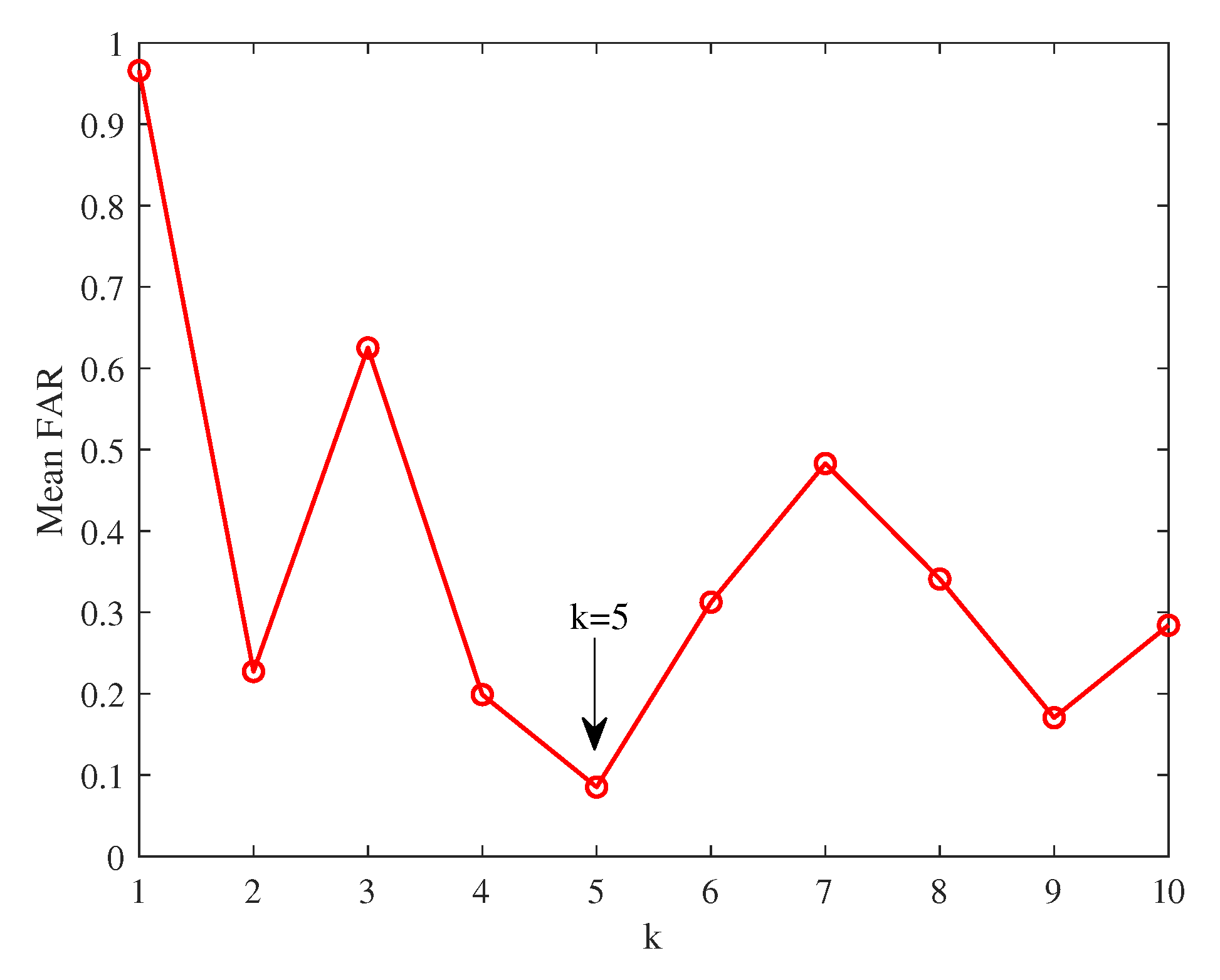
Figure 2.
Grid search result of the fusion weights and for the TE process.
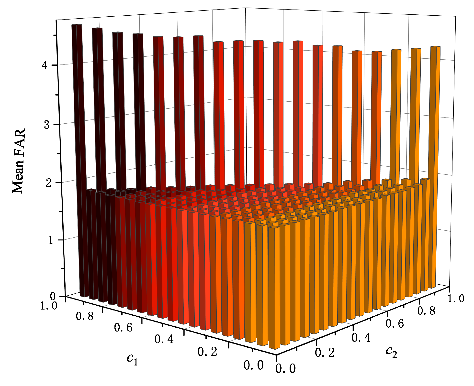
Figure 3.
Monitoring results for the fault 10: TE process.
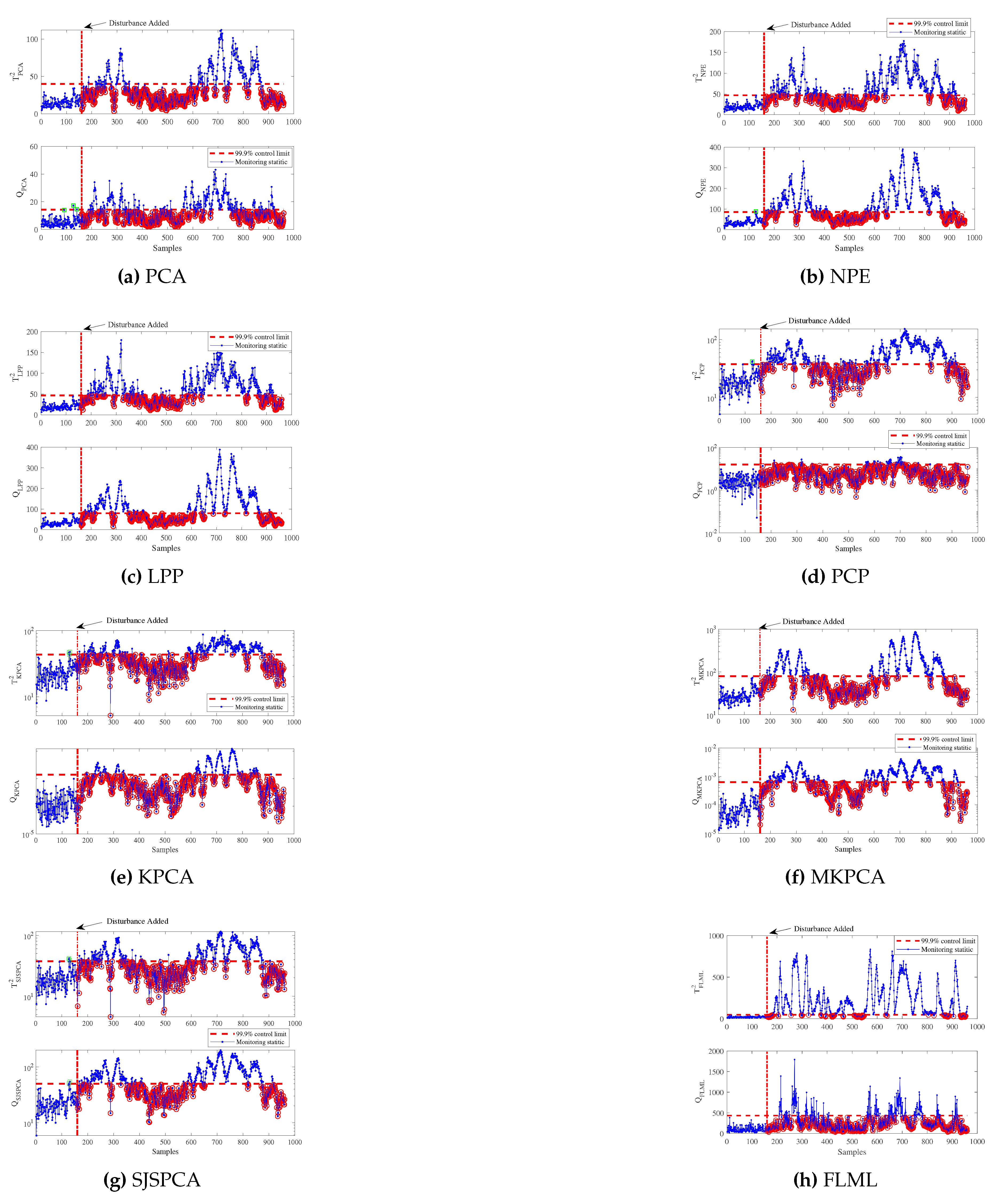
Figure 4.
Monitoring results for the fault 19: TE process.
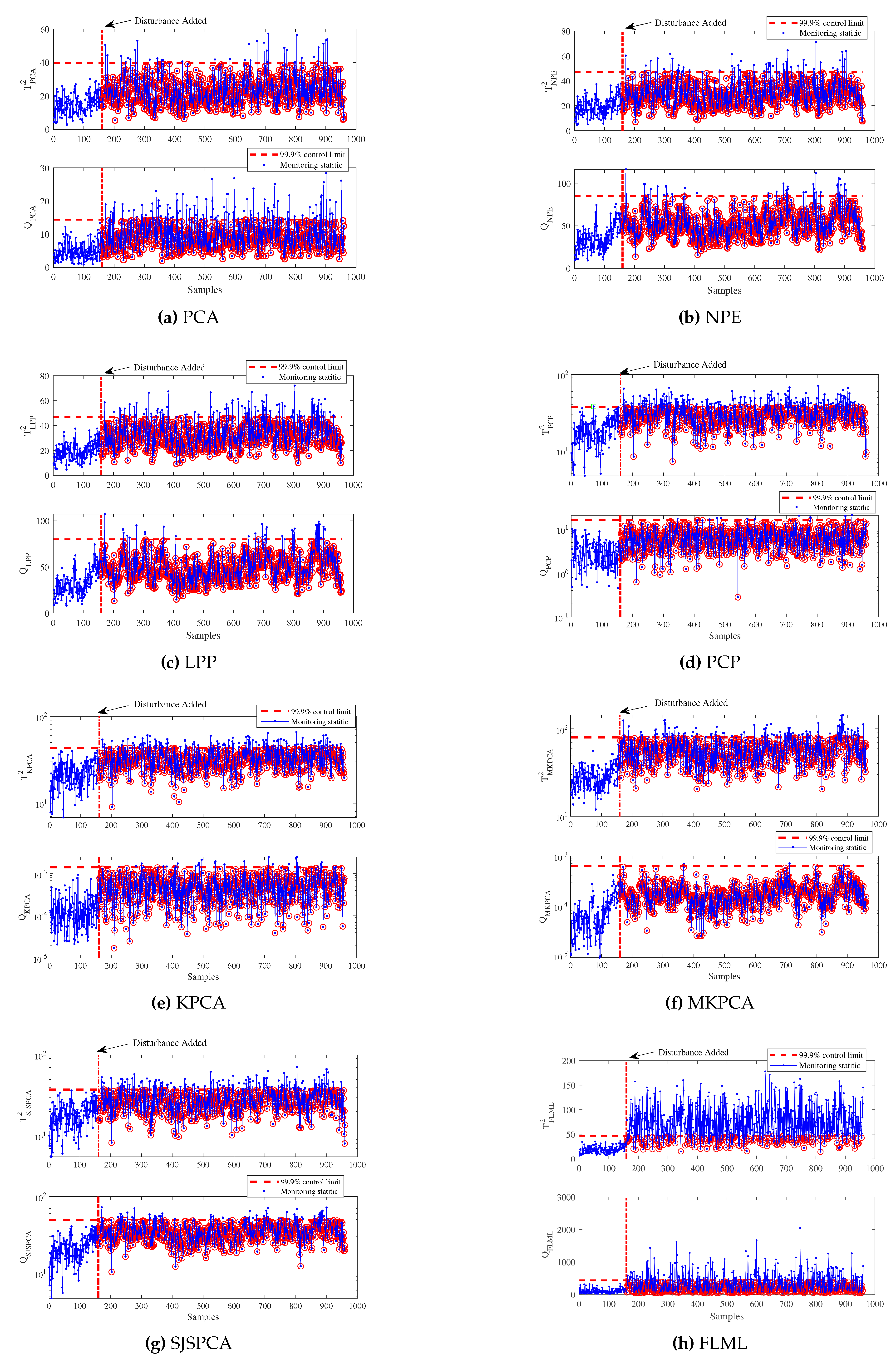
Figure 6.
Grid search result of the fusion weights and for the blast furnace ironmaking process.
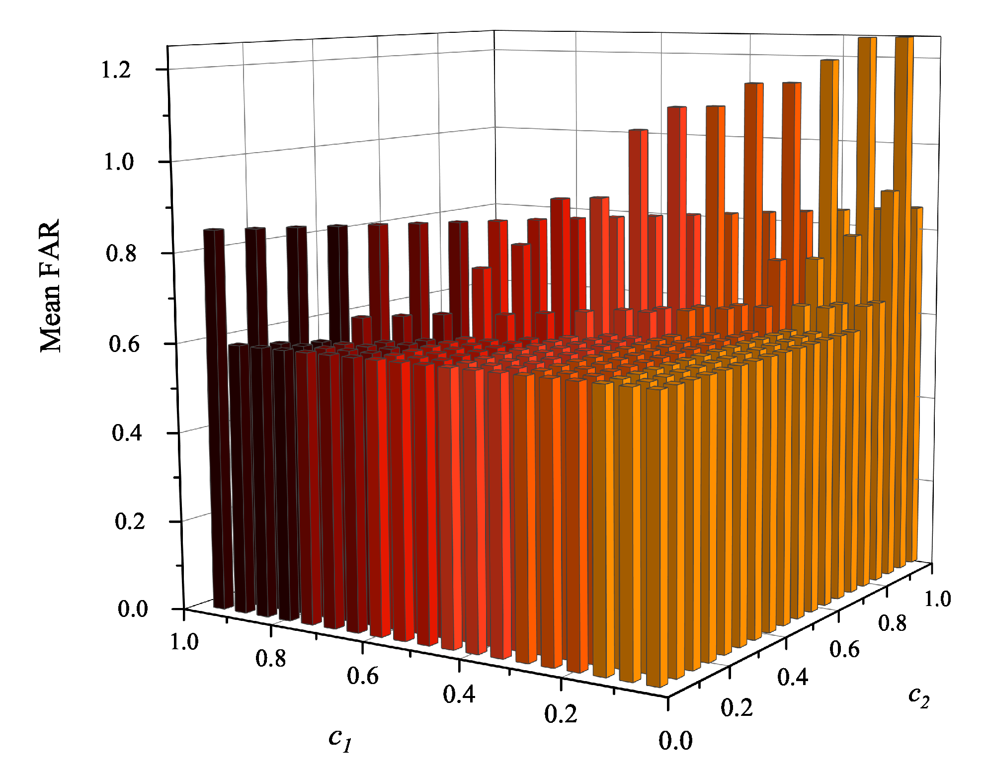
Figure 7.
Monitoring results for the channeling condition: blast furnace ironmaking process.
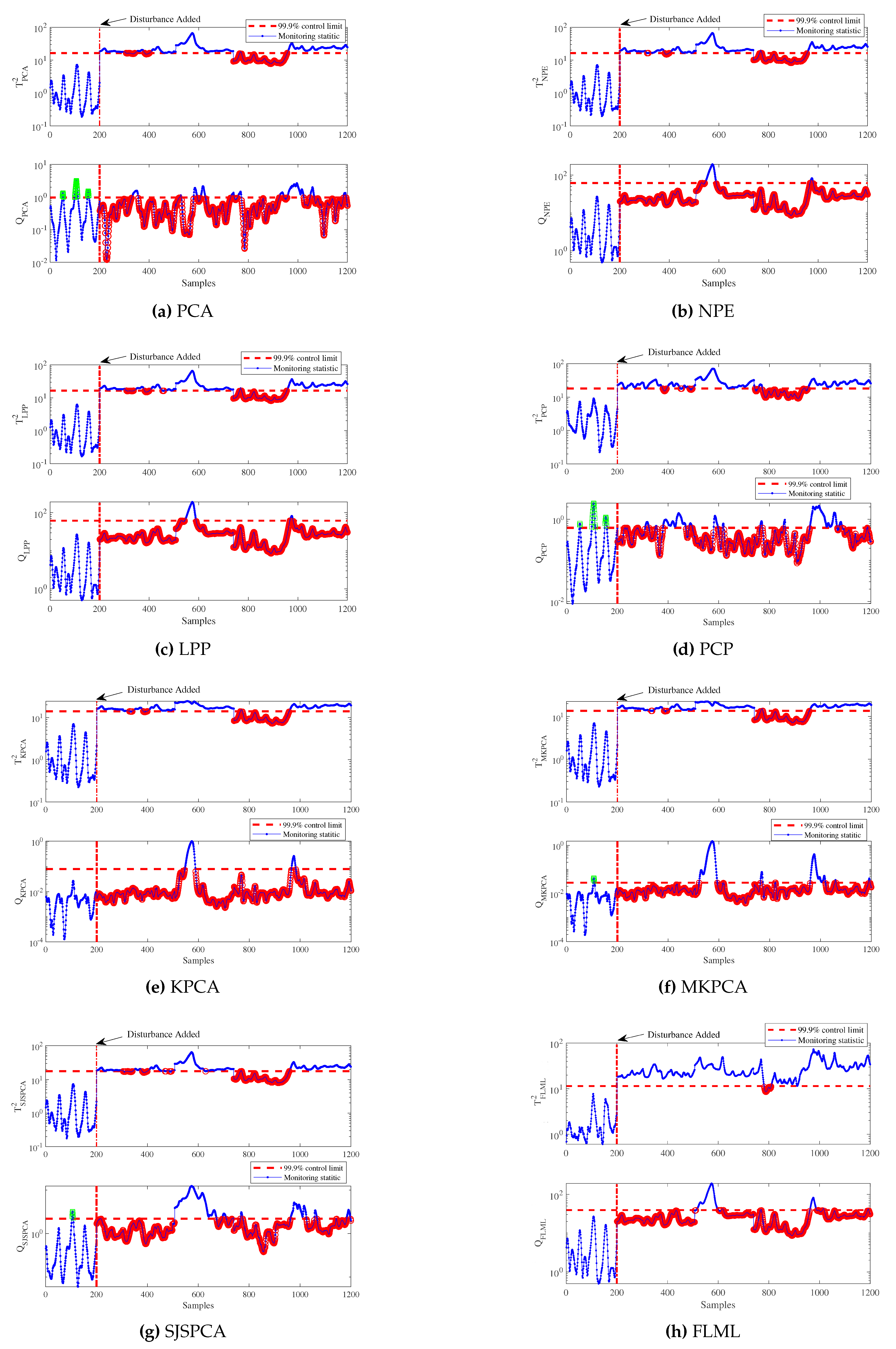

Table 1.
Faults description of the TE process.
| No. | Fault description | Fault type |
| IDV(0) | Normal situations | - |
| IDV(1) | A/C feed ratio, B composition constant (Stream 4) | Step |
| IDV(2) | B composition, A/C ratio constant (Stream 4) | Step |
| IDV(4) | Reactor cooling water inlet temperature | Step |
| IDV(5) | Condenser cooling water inlet temperature | Step |
| IDV(6) | A feed loss (Stream 1) | Step |
| IDV(7) | C header pressure loss-reduced availability (Stream 4) | Step |
| IDV(8) | A, B, C feed composition (Stream 4) | Random variation |
| IDV(10) | C feed temperature (Stream 4) | Random variation |
| IDV(11) | Reactor cooling water inlet temperature | Random variation |
| IDV(12) | Condenser cooling water inlet temperature | Random variation |
| IDV(13) | Reaction kinetics | Slow drift |
| IDV(14) | Reactor cooling water valve | Sticking |
| IDV(16) | Unknown | Unknown |
| IDV(17) | Unknown | Unknown |
| IDV(18) | Unknown | Unknown |
| IDV(19) | Unknown | Unknown |
| IDV(20) | Unknown | Unknown |
| IDV(21) | Valve fixed at steady-state position | Constant position |
Table 2.
Comparison results of MDR values for TE process.
| No. | PCA | NPE | LPP | PCP | KPCA | MKPCA | SJSPCA | FLML | ||||||||
| Q | Q | Q | Q | Q | Q | Q | Q | |||||||||
| 1 | ||||||||||||||||
| 2 | ||||||||||||||||
| 4 | ||||||||||||||||
| 5 | ||||||||||||||||
| 6 | ||||||||||||||||
| 7 | ||||||||||||||||
| 8 | ||||||||||||||||
| 10 | ||||||||||||||||
| 11 | ||||||||||||||||
| 12 | ||||||||||||||||
| 13 | ||||||||||||||||
| 14 | ||||||||||||||||
| 16 | ||||||||||||||||
| 17 | ||||||||||||||||
| 18 | ||||||||||||||||
| 19 | ||||||||||||||||
| 20 | ||||||||||||||||
| 21 | ||||||||||||||||
| Aver. | ||||||||||||||||
Table 3.
Comparison results of FAR values for TE process.
| No. | PCA | NPE | LPP | PCP | KPCA | MKPCA | SJSPCA | FLML | ||||||||
| Q | Q | Q | Q | Q | Q | Q | Q | |||||||||
| 1 | ||||||||||||||||
| 2 | ||||||||||||||||
| 4 | ||||||||||||||||
| 5 | ||||||||||||||||
| 6 | ||||||||||||||||
| 7 | ||||||||||||||||
| 8 | ||||||||||||||||
| 10 | ||||||||||||||||
| 11 | ||||||||||||||||
| 12 | ||||||||||||||||
| 13 | ||||||||||||||||
| 14 | ||||||||||||||||
| 16 | ||||||||||||||||
| 17 | ||||||||||||||||
| 18 | ||||||||||||||||
| 19 | ||||||||||||||||
| 20 | ||||||||||||||||
| 21 | ||||||||||||||||
| Aver. | ||||||||||||||||
Table 4.
Comparison results of DD values for TE process.
| No. | PCA | NPE | LPP | PCP | KPCA | MKPCA | SJSPCA | FLML | ||||||||
| Q | Q | Q | Q | Q | Q | Q | Q | |||||||||
| 1 | ||||||||||||||||
| 2 | ||||||||||||||||
| 4 | ||||||||||||||||
| 5 | ||||||||||||||||
| 6 | ||||||||||||||||
| 7 | ||||||||||||||||
| 8 | ||||||||||||||||
| 10 | ||||||||||||||||
| 11 | ||||||||||||||||
| 12 | ||||||||||||||||
| 13 | ||||||||||||||||
| 14 | ||||||||||||||||
| 16 | ||||||||||||||||
| 17 | ||||||||||||||||
| 18 | ||||||||||||||||
| 19 | ||||||||||||||||
| 20 | ||||||||||||||||
| 21 | ||||||||||||||||
| Aver. | ||||||||||||||||
Table 5.
Variable description of the Blast furnace ironmaking process.
| No. | Variable description | Unit |
| 1 | Oxygen enrichment rate | % |
| 2 | Enriching oxygen flow | |
| 3 | Hot blast temperature | C |
| 4 | Top temperature(1) | C |
| 5 | Top temperature(2) | C |
| 6 | Top temperature(3) | C |
| 7 | Downcomer temperature | C |
Table 6.
Comparison results of MDR, FAR and DD values for blast furnace ironmaking process.
| PCA | NPE | LPP | PCP | KPCA | MKPCA | SJSPCA | FLML | ||||||||
| Q | Q | Q | Q | Q | Q | Q | Q | ||||||||
| a | |||||||||||||||
| b | |||||||||||||||
| c | |||||||||||||||
a First row: Missed Detection Rates (MDR, %). b Second row: False Alarm Rates (FAR, %). c Third row: Detection delays(DD, mins).
Disclaimer/Publisher’s Note: The statements, opinions and data contained in all publications are solely those of the individual author(s) and contributor(s) and not of MDPI and/or the editor(s). MDPI and/or the editor(s) disclaim responsibility for any injury to people or property resulting from any ideas, methods, instructions or products referred to in the content. |
© 2023 by the authors. Licensee MDPI, Basel, Switzerland. This article is an open access article distributed under the terms and conditions of the Creative Commons Attribution (CC BY) license (http://creativecommons.org/licenses/by/4.0/).
Copyright: This open access article is published under a Creative Commons CC BY 4.0 license, which permit the free download, distribution, and reuse, provided that the author and preprint are cited in any reuse.


