1. Introduction
Asphaltene solid particles can precipitate due to changes in thermodynamic properties, such as pressure, temperature, and composition (Renpu, 2011; Alhosani and Daraboina, 2020; Enayat et al., 2020). Precipitates of asphaltene in oil reservoirs or in pipelines could cause many flow assurance problems (Hassanpouryouzband et al., 2020). To minimize this risk, it is necessary to determine when asphaltene begins to precipitate and at which thermodynamic conditions (Buriro and Shuker, 2013; Fakher et al., 2020; Shirani et al., 2012). Predicting the onset pressure of asphaltene transport may aid in the effective management of oil field production facilities. It will result in improved reservoir management by designing stimulation jobs in a timely manner to minimize the formation damage caused by asphaltene. The perturbed-chain statistical associated fluid theory (PC SAFT) and Peng-Robinson equations of state are the most frequently used thermodynamic models for predicting the onset pressure (Gross and Sadowski, 2001; Peng and Robinson, 1976). Predicting the asphaltene pressure onset using the PC SAFT equation of state (EOS) or the Peng-Robinson is a complex and time-consuming procedure (Gonzalez et al., 2005; Hosseinzadeh et al., 2018; Abutaqiya et al., 2020; Seitmaganbetov et al., 2021). The complexity arises from the fact that both the PC SAFT and Peng-Robinson equations of state have multiple adjustable parameters, such as the critical properties of asphaltene and resins in the Peng-Robinson equation of state, or segment number (m), segment diameter (σ), and segment–segment interaction energy (ε/k) of the asphaltene and resins, which are PC SAFT parameters. By modifying the asphaltene critical properties using the Peng-Robinson equation of state, the experimental precipitation onset pressure can be matched with the predicted onset pressure. Even after such precise tuning, the predicted asphaltene onset pressure exhibits large errors at very low or very high temperatures (Seitmaganbetov et al., 2021). Furthermore, the saturates, aromatics, resins, and asphaltene (SARA)-based characterization procedure is required for the accurate modeling of the asphaltene onset pressure (Abutaqiya et al., 2020). This characterization procedure requires flashing the live oil into gas and dead oil. Later, a recombination calculation is required to convert the carbon-based composition to a SARA fraction-based composition. The selection of binary interaction parameters has a profound effect on asphaltene onset pressure modeling using the equation of state (Buriro and Imqam, 2021). As of today, there is no correlation for a SARA-based crude oil composition that can predict the binary interaction parameters accurately. Additionally, the inaccurate selection of binary interaction parameters may lead to high errors in asphaltene onset pressure prediction modeling.
Given the complexity of equation of state modeling and the requirement for parameter tuning, a direct thermodynamic model is required that does not need parameter tuning but still predicts the onset pressure accurately. Few regression-based models have previously been developed to provide a direct and rapid prediction of the asphaltene onset pressure during pressure depletion, including the two most common multivariate models developed by Fahim (2007) and Ameli et al. (2016). Fahim (2007) proposed three distinct models for correlating the upper and lower onset pressures as well as the saturation pressure. However, that developed model used insufficient data points and linear multivariate regression analysis, which make the validity and accuracy of the model questionable. The upper onset pressure model contains 17 independent variables, making it lengthy and complex. Statistically, no multicollinearity test was included, which casts doubt on the use of the independent parameters. Overfitting occurs when there are too many parameters and a small training data set. Such models can be applied to specific data sets but are incapable of prediction (Lever, 2016). Ameli et al. (2016) developed a new upper onset pressure model to compensate for the inaccuracies of the Fahim (2007) model, employing two constrained multivariable search methods, namely, generalized reduced gradient (GRG) and successive linear programming (SLP). However, the model retains 17 independent variables, and the development and training data sets are limited.
Using a multivariate linear regression model, this work will develop a simple and accurate thermodynamic model for predicting the upper precipitation onset pressure under pressure depletion at various temperatures. Ninety-four experimental data points from 37 published crude oil data sets were collected. To assess the model’s accuracy and validity, the results were compared to experimental data, the PC SAFT equation of state, the Peng-Robinson equation of state, Fahim's model, and Ameli et al.’s model. The current study will also evaluate the accuracy of Fahim’s model, and Ameli et al.’s regression-based models by comparing their prediction results with experimental data. Statistical measures (i.e., relative error and absolute error) were used to compare the developed model’s performance to that of the other models mentioned.
1.1. Modelling of the asphaltene precipitation phase envelope
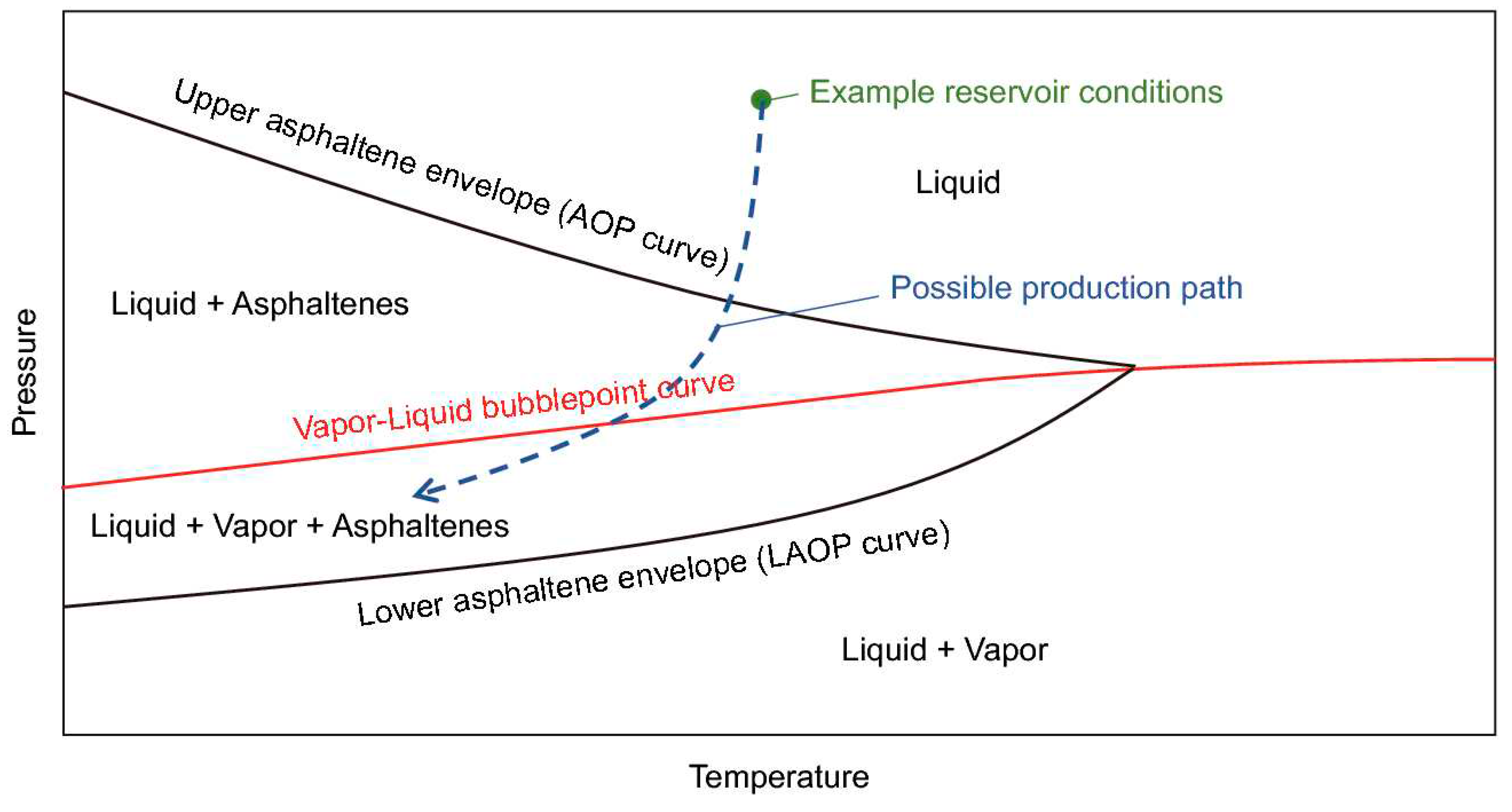
A pressure-temperature (PT) diagram is frequently used to depict the thermodynamic properties of asphaltene (Jamaluddin et al., 2012). At a given temperature, the asphaltene precipitation onset pressure is defined as the pressure at which asphaltene begins to precipitate. The temperature being considered is either at the reservoir or the wellbore. The temperature directly affects the onset pressure, and as the temperature changes, the asphaltene onset pressure also changes. As illustrated in Figure 1, the asphaltene phase envelope is divided into four regions: (1) liquid only, (2) liquid+asphaltene, (3) liquid+vapor+asphaltene, and (4) liquid+vapor.
There are two regions above the vapor-liquid bubble point curve: the liquid-only and liquid+asphaltene regions. The upper asphaltene envelope (or asphaltene-precipitation onset pressure (UAOP) separates the liquid-only region from the liquid+asphaltene region. Asphaltene does not precipitate in the liquid-only area, but it does precipitate in the liquid+asphaltene area when the pressure or temperature is lowered. As the pressure and temperature further changes and falls below the vapor-liquid bubble curve, the composition of the oil starts to change as a result of gas being liberated from the crude oil. Therefore, asphaltene precipitation is a function of the composition and pressure in the liquid+vapor+asphaltene region. Lower asphaltene onset pressure (LAOP) is the liquid+vapor+asphaltene region’s boundary-line curve. The liquid+vapor region is located below this line. As solution gas is withdrawn from the oil in this region, the oil becomes denser, allowing previously precipitated asphaltenes to re-solubilize. As a result, there is no asphaltene precipitation in this area.
The current study focused on investigating asphaltene precipitation in the liquid+asphaltene region, where the temperature and pressure were the main two factors impacting the asphaltene precipitation and flocculation under depletion conditions.
Figure 1.
Asphaltene phase envelope (Shoukry et al., 2020).
Figure 1.
Asphaltene phase envelope (Shoukry et al., 2020).
2. Materials and Methods
The optimal model was developed in five stages (Figure 2). The first step was to create a thermodynamic database for the asphaltene experimental data. Step two involved forming a multicollinearity test on the data in the database. Step three created data frequency histograms to determine the range of the available data. In step four, data analysis was performed to ascertain the trends in the data sets. Finally, in step five, asphaltene thermodynamic models were developed through multicollinearity testing, histogram analysis, and data analysis.
Figure 2.
Asphaltene onset pressure model development flow diagram.
Figure 2.
Asphaltene onset pressure model development flow diagram.
2.1. Crude oil database
A total of 94 data points were gathered from the published literature for 37 crude oils. Eighteen crude oil data sets containing 59 data points were used to train the model, as detailed in Table A2 (Appendix). The remaining 35 experimental data points were used to test the developed model, as detailed in Table A3 (Appendix). The experimental data that were collected to develop the asphaltene onset pressure prediction model included (1) saturates, aromatics, resins, and asphaltenes (SARA) analysis, (2) experimental asphaltene onset pressure, and (3) experimental bubble point pressure.
2.2. Multicollinearity test
In general, the multicollinearity test estimates correlations between two or more predictor variables. In other words, one predictor variable can predict another predictor variable. This creates extra data, which alters the regression model’s results. Therefore, removing multicollinear parameters is crucial. The collinearity threshold between two predictors is kept between 0.5 and –0.5. (Dormann et al., 2013). The collinearity test considers the following parameters: resins (R), saturate-to-aromatic ratio (SA), temperature (t), bubble point pressure (Pb), nitrogen (N2), carbon dioxide (CO2), methane (C1), ethane (C2), propane (C3), and heavy gas fraction (C4+).
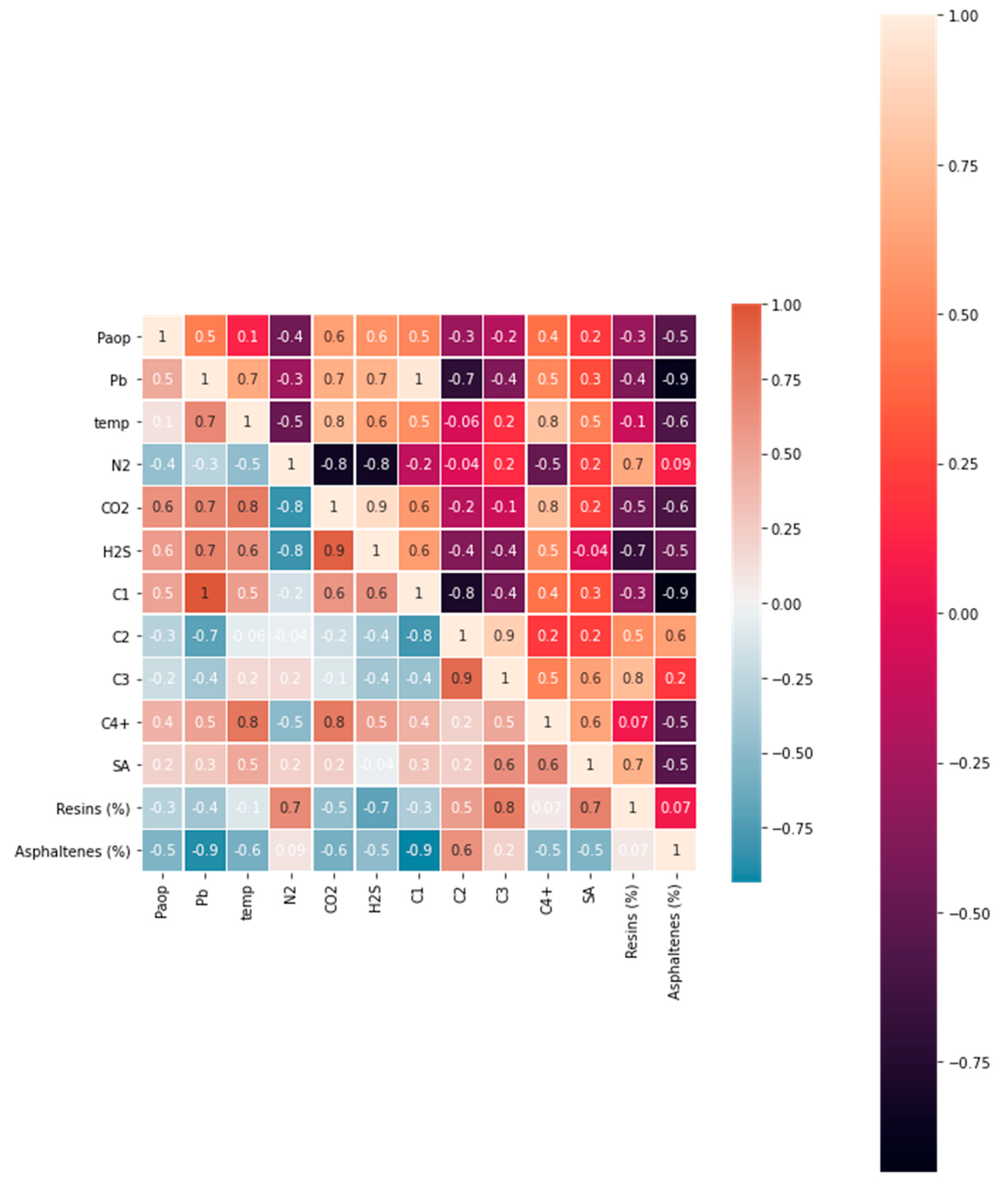
Figure 3 depicts a heatmap of correlations between variables derived from the published experimental data in Table A2 (Appendix). The heatmap was created using the Python programming language’s Seaborn library (SNS heatmap). The results indicated that multicollinearity was present in C1, C2, C3, C4+, N2, H2S, asphaltene, and CO2. For instance, C1 had a correlation coefficient greater than 0.5 with Pb, CO2, and H2S, but less than –0.5 with asphaltene and C2. The correlation coefficient between asphaltene and the bubble point pressure was less than –0.5. Thus, C1, C2, C3, C4+, N2, CO2, H2S, and asphaltene predictors could be eliminated due to multicollinearity issues.
The temperature, bubble point pressure, saturate-to-aromatic ratio (SA), and resins were chosen as the primary predictors for the upper onset pressure model. The saturate-to-aromatic ratio had a collinearity of less than 0.5 with the bubble point pressure and resins but had an acceptable collinearity of 0.5 with the temperature. Resin had a collinearity of less than –0.5 with the bubble point pressure and temperature but 0.7 with resins. Although the temperature had a low negative correlation with resin and the saturate-to-aromatic ratio, temperature had a strong correlation with the bubble point pressure, with a coefficient of 0.7. Because the experimental data in the Appendix demonstrated that the temperature and bubble point pressure had a direct effect on the onset pressure, both were considered continuous predictors. As a result, both predictors were treated as independent variables in the development of the model.
Figure 3.
Multicollinearity heatmap.
Figure 3.
Multicollinearity heatmap.
2.3. Physical significance of parameters
Numerous researchers have discussed the role of saturates, aromatics, resins, and asphaltene in the destabilization of solid particles. Mousavi et al. (2016) investigated the effect of resin on the precipitation of asphaltene. Their calculations indicated that when both asphaltene and resin are present, resin-asphaltene interactions were preferable to asphaltene–asphaltene interactions only when the number of resin molecules per micelle exceeded the number of asphaltene molecules per micelle. As the crude became heavier, the proportion of lighter saturates (alkanes) typically decreased (Mansoori, 2009). Also, excess aromatics in crude oil in contact with asphaltene may result in the formation of micelles (Mansoori, 1996a). Chukwuemeka et al. (2017) investigated the saturate-to aromatic ratios in three crude oil samples collected from Kokori, Afiesere, and Nembe in the Niger Delta region, Nigeria. All three were found to be light. Chukwuemeka et al. (2017) compared the saturate-to-aromatic ratio with heptane-induced asphaltene precipitation. Their study found that the lowest saturate-to-aromatic ratio led to a highest asphaltene precipitation. They concluded that when comparing different crude oils in terms of the amount of asphaltenes present in them, using their saturate saturate-to-aromatic ratio is a very efficient method. Additionally, fundamental thermodynamic properties, such as reservoir pressure and temperature, can cause asphaltene particles to destabilize above the bubble point pressure (Omid et al., 2019). Table 1 summarizes the parameters selected to develop the model based on findings from the multicollinearity heatmap (Figure 3). This work employed only continuous predictor types. Continuous variables are those that can take on an infinite number of real values within a given interval.
Table 1.
Parameters used to develop the model.
Table 1.
Parameters used to develop the model.
| |
Fitting Parameters |
Predictor Type |
| 1. |
Bubble Point Pressure, psi |
Continuous |
| 2. |
Temperature, oF |
Continuous |
| 3. |
Saturate-to-Aromatic Ratio (S/A), % |
Continuous |
| 4. |
Resins, % |
Continuous |
2.4. Data frequency histograms
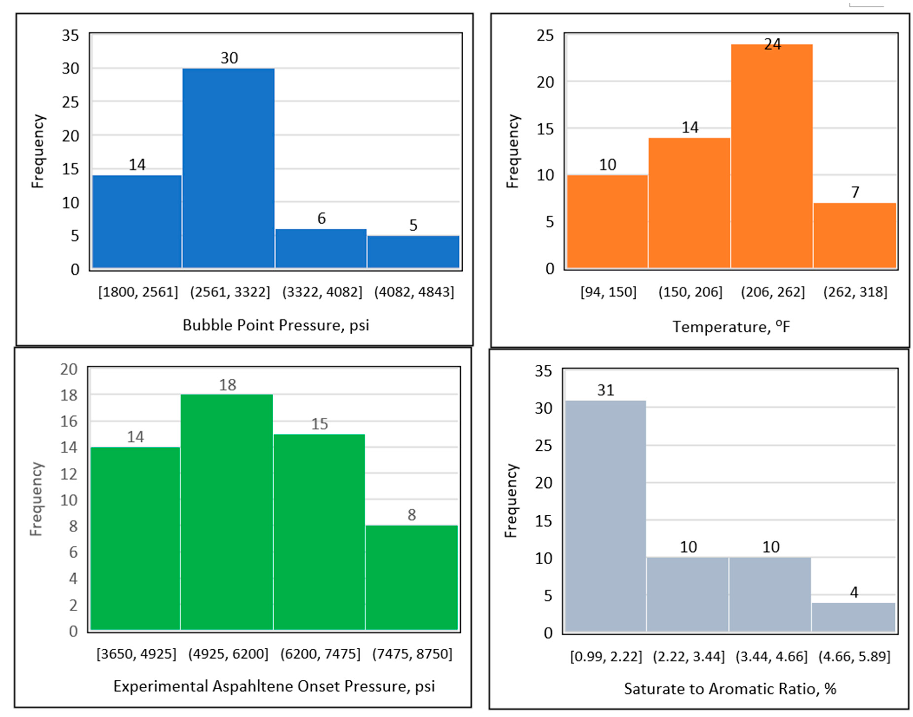
Figure 4 shows the data distribution of the temperature, bubble point pressure, experimental onset pressure, and saturate-to-aromatic ratio. The temperature data ranged between 94 and 300℉, but predominantly lay between 150 and 262℉. The data for the experimental precipitation onset pressure ranged from 3200 to 9000 psi, with most of the experimental precipitation onset pressure data points found between 4650 and 7500 psi. The bubble point pressure fell between 1800 and 4082 psi, with the majority of the bubble point pressure data points found between 2000 and 3500 psi. Finally, the ratio of saturates to aromatics varied between 0.99 and 5.89%, with and the majority of the saturate-to-aromatic ratio data points falling between 0.99 and 4.66%.
Figure 4.
Data distribution using histogram plots.
Figure 4.
Data distribution using histogram plots.
2.5. Asphaltene onset pressure data analysis
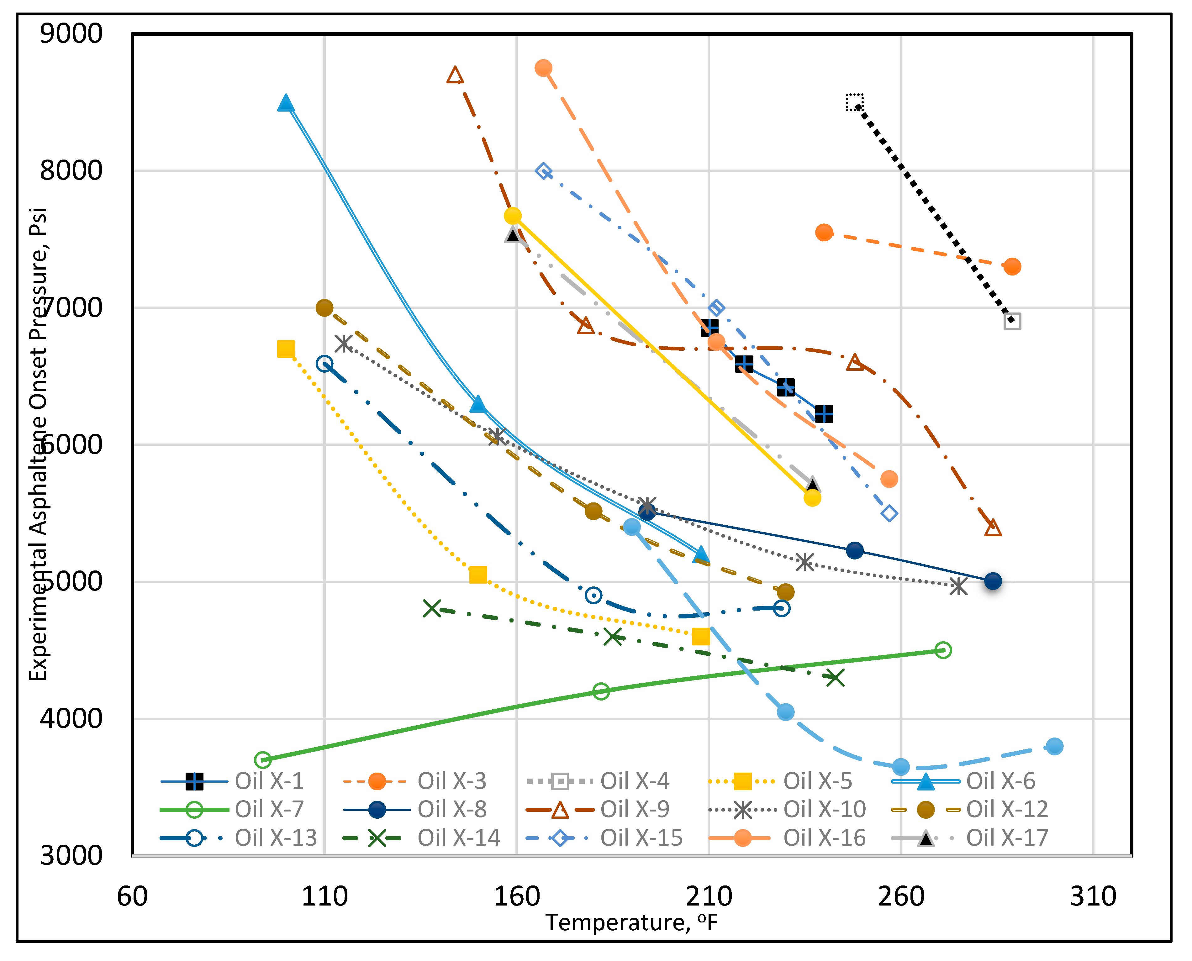
Asphaltene onset pressure and other experimental data are provided for each crude oil in Table A2 (Appendix). Each crude oil was assigned a unique name beginning with “Oil X” and ending with a number. The experimental data demonstrated that the asphaltene onset pressure varied significantly with temperature. Therefore, temperature vs. asphaltene onset pressure was plotted for 19 crude oil data sets, as shown in Figure 5. The data are very diverse, nonlinear, and do not follow any clear trend. For example, at 100°F, Oil X-6 had an onset pressure of 8500 psi, while Oil X-5 had an onset pressure of 6700 psi, and Oil X-7 had an onset pressure of 3800 psi. At 212°F, Oil X-1’s onset pressure was 6854 psi, Oil X-2’s was 5299 psi, Oil X-16’s was 6750 psi, and Oil X-5’s was 4600 psi. It can be seen that the changes in the onset pressure with temperature do not follow a linear trend, but rather a curvilinear trend, for the majority of the oils. This could have occurred because the extracted data were obtained from laboratory research work that each had a distinct pattern of results. We also understand that the discrepancy in the data could be caused by inaccurate laboratory measurements. The solution to using such disparate data is to determine the hidden patterns and to group them together (Rokach and Maimon, 2005). In conclusion, because the asphaltene onset pressure data exhibit such a wide range of values at each relevant temperature, asphaltene onset pressure data were sorted using clustering techniques to group them with data that exhibited similar behavior.
Figure 5.
Temperature vs. experimental asphaltene onset pressure.
Figure 5.
Temperature vs. experimental asphaltene onset pressure.
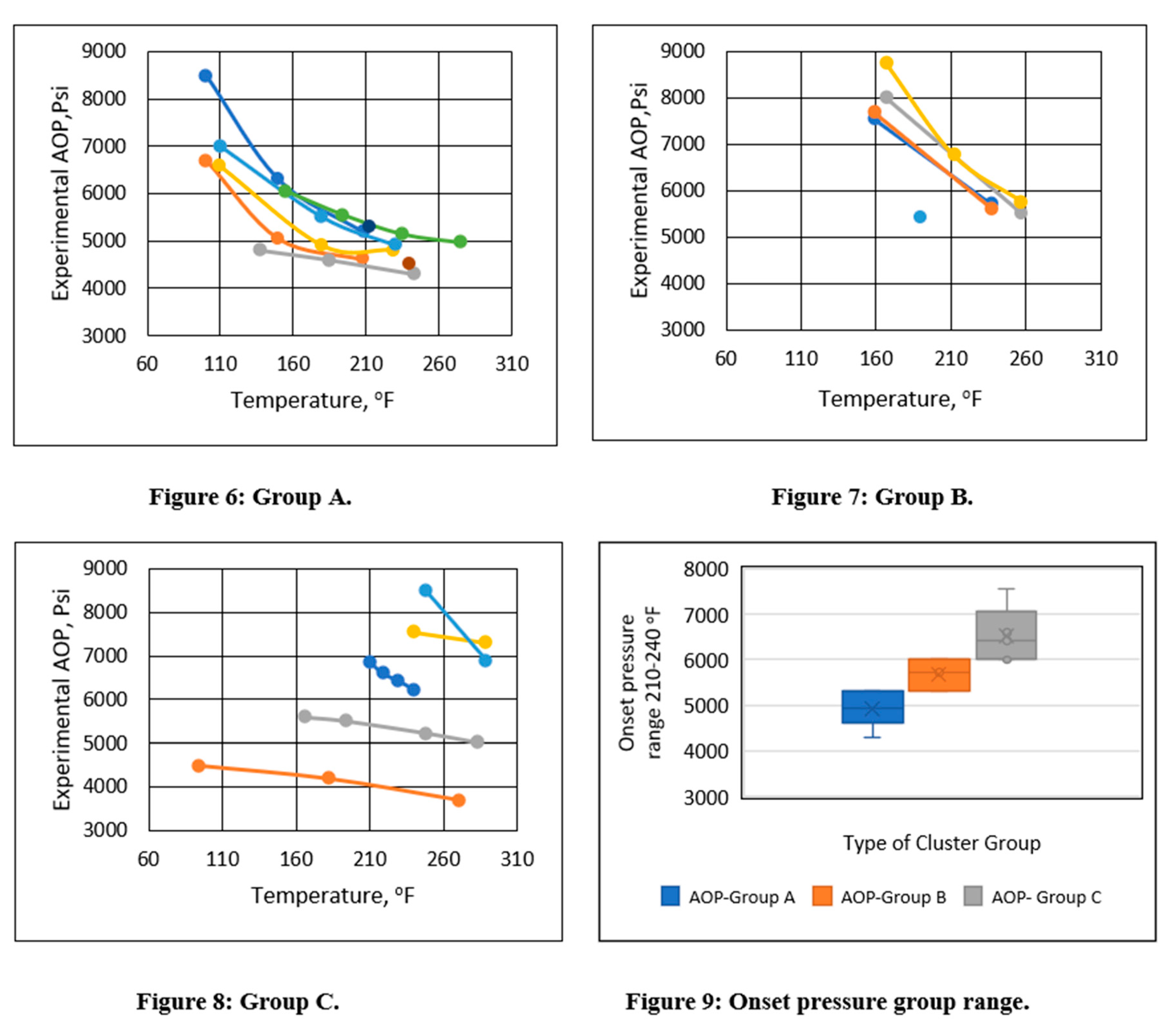
Subgroups were formed based on the asphaltene onset pressure in the temperature range of 200-240°F in an unsupervised manner. Three distinct asphaltene onset pressure vs. temperature trends were identified, as shown in Figures 6-8. Groups were formed based on the experimental onset pressure range and are summarized in Table 2. These three distinct patterns exhibited both linear and polynomial characteristics. As a result, regression analysis could be used to analyze them. The box plot in Figure 9 indicates that Group A’s onset pressure range was between 4000 and 5300 psi, Group B’s range was between 5300 and 6000 psi, and Group C’s range was between 6000 and 7300 psi.
Table 2.
Asphaltene onset pressure cluster ranges.
Table 2.
Asphaltene onset pressure cluster ranges.
| Name |
Experimental asphaltene onset pressure cluster range |
Asphaltene onset pressure trend performance |
| Group A |
Less than 5300 psi |
Curvilinear |
| Group B |
From 5300 to 6000 psi |
Curvilinear |
| Group C |
Greater than 6000 psi |
Curvilinear |

2.6. Asphaltene onset pressure model development
2.6.1. Introduction to multivariate regression models
Multiple linear regression attempts model the relationship between two or more explanatory variables and a response variable by fitting a linear equation to the observed data. Every value of the independent variable X is associated with a value of the dependent variable Y (Pinder, 2017).
Formally, the model for multiple linear regression, given n observations, is
where
is the predicted or expected value of the dependent variable, X
1 through X
p are p distinct independent or predictor variables, b
0 is the value of Y when all of the independent variables (X
1 through X
p) are equal to zero, and b
1 through b
p are the estimated regression coefficients.
Polynomial regression is a special case of linear regression where a polynomial equation is fit to the data with a curvilinear relationship between the target variable and the independent variables. In a curvilinear relationship, the value of the target variable changes in a nonuniform manner in relation to the predictor(s). A polynomial regression equation of degree
n is written as follows:
where
is the bias,
, , …, are the weights in the equation of the polynomial regression, and
n is the degree of the polynomial. The number of higher-order terms increases as the value of
n increases; hence, the equation becomes more complicated.
Relative error can be calculated from the following equation, where E
i% is the relative deviation of a predicted value from an experimental one and is introduced as the percent relative error:
where
is the original experimental value, and
is the predicted value.
Clustering, also known as cluster analysis, is a machine learning technique that groups unlabeled data. It is defined as “a method for classifying data points into distinct clusters comprised of similar data points. The objects with possible similarities are retained in a group that bears little or no resemblance to another
” (Rokach & Maimon, 2005). The model was chosen using the standard error of the regression (
S), the predicted and adjusted R
2 values, and Mallow's coefficient of determination (Cp). Mallow’s Cp is a metric used to select the optimal regression model among several models. It is calculated as
where
is the residual sum of squares for a model with
p predictor variables; S
2 is the residual mean square for the model (estimated by the mean squared error or MSE); n is the sample size; and P is the number of predictor variables.
Mallow’s Cp is used when there are several potential predictor variables to include in a regression model and the goal is to identify the best model that incorporates a subset of these variables. The optimal regression model has the lowest Cp value that is less than or equal to P+1, where P is the number of predictor variables in the model.
The standard error of the regression (S), alternatively referred to as the standard error of the estimate, is a measure of the average distance between the observed values and the regression line. Conveniently, it indicates how far off the mark the regression model is, on average, when the response variable’s units are used. Smaller values are preferable because they indicate that the observations were more closely associated with the fitted line. Complete theoretical details are available in the original references (Minitab, LLC, 2019). The analysis of variance was performed using the P-value and T-value. The theoretical foundations of variance analysis are available from the original source (Minitab, LLC, 2019). When the pressure exceeded the bubble point, it was assumed that the asphaltene precipitation onset pressure was a function of only the pressure and temperature.
Temperature plotted against the onset pressure exhibited a curvilinear relationship, as illustrated in
Figure 5. As a result, the model was developed using polynomial regression. Previously, in
Section 2.2, pressure, temperature, saturate-to-aromatic ratio, and resin were identified as continuous predictors. Polynomial regression requires taking the square of selected predictors. Therefore, temperature squared (t
2), bubble point pressure squared (P
b2), and the bubble point pressure and temperature product (Pb*t) were introduced to make the expression a polynomial regression. Subset analysis was used to determine the most effective set of predictors. The subset model was chosen based on the model’s Mallow’s Cp, S, and adjusted R
2 values. The
Appendix contains the subset analysis for the models.
2.6.2. Asphaltene onset pressure prediction model
Based on the analysis of the Mallow’s Cp, S, and adjusted R
2 values
(Table A4,
Table A5 and
Table A6, Appendix), three models were developed based on the identified cluster group in section 2.4. Those are named Model 1a, Model 1b, and Model 1c. A summary of the developed selected models is provided in
Table 3 and
Table 4. The adjusted R
2 for Model 1a is 95.0%; for Model 1b, is 96.57%, and for Model 1c, is 97.22%. The models were selected from the subset analysis given in
Table A4,
Table A5 and
Table A6 (
Appendix), with lower S values, higher predicted R
2 values, higher adjusted R-squared values, and Mallow’s Cp. The adjusted R
2 suggests that the models are well fitted with the training data and are ready to predict the onset pressure based on a similar trend.
Table 3.
Developed selected models.
Table 3.
Developed selected models.
| Name |
Equation |
| Model 1a |
|
|
Conditions to use: if asphaltene onset pressures are less than 5300 psi |
| Model 1b |
|
|
Conditions to use: if asphaltene onset pressures are greater than 5300 and less than 6000 psi |
| Model 1c |
|
|
Conditions to use: if asphaltene onset pressures are greater than 6000 and less than 10000 psi |
Table 4.
Selected model summary.
Table 4.
Selected model summary.
| |
Mallow’s Cp |
S |
R2
|
R2 (adj) |
R2 (pred) |
| Model 1a |
7.9 |
233.253 |
96.1% |
95.0% |
90.5% |
| Model 1b |
4.1 |
304.154 |
98.00% |
96.57% |
92.16% |
| Model 1c |
4 |
223.682 |
98.21% |
97.22% |
95.25% |
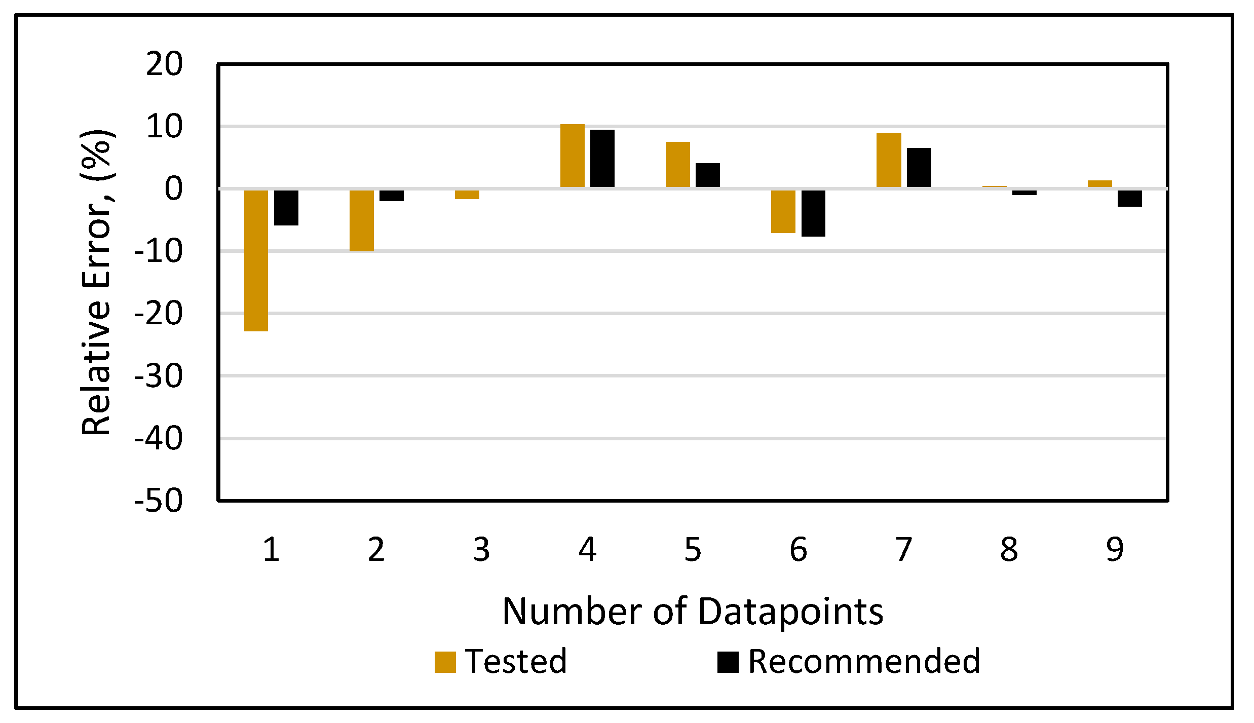
The analysis of variance results are provided in Table 5. Model 1a had four predictors: temperature, temperature squared, bubble point pressure, and squared bubble point pressure. The P-value for all of the predictors was less than 0.05. Therefore, it was concluded that all parameters were statistically significant in Model 1a. Additional subsets from Table A4 (Appendix) were examined to see how well they predicted the testing data set. Despite a higher R2 of 91.3, the result of subset no. 9 yielded a higher error than the recommended model, as shown in Figure A1 (Appendix). As a result, the best model (Model 1a) is recommended based on the model’s superior prediction capabilities.
Model 1b had five predictors: resins, temperature squared, temperature, and product of bubble point pressure and temperature. The P-value for all of the predictors was less than 0.05, except for the bubble point pressure. The model without Pb2 is given in subset no. 8 in Table A5 (Appendix). The result indicate that the model had an S value of 337.12, a Mallow’s Cp of 4.2, and an adjusted R2 (pred) of 91.7%, while the model with Pb2 given in subset no. 9 had an S value of 304.15, a Mallow’s Cp of 4.1, and an adjusted R2 (pred) of 92.2%. Analysis indicated that the model with Pb2 had a lower S value and higher predicted R2. Therefore, the model with Pb2 was selected and evaluated against the testing data.
Model 1c had six predictors: resins, saturate-to-aromatic ratio, temperature, temperature squared, bubble point pressure, product of bubble point pressure and temperature. The P-value for all of the predictors was less than 0.05, except for temperature. The model without temperature was given in subset no. 8 in Table A6 (Appendix). The results indicated that the model without temperature had an S value of 316.15, a Mallow’s Cp of 10.5, and an adjusted R2 of 90.4, while the model with temperature given in subset no. 9 in Table A6 (Appendix) had an S value of 223.68, a Mallow’s Cp of 4, and an adjusted R2 of 95.3%. The analysis of both sets indicated that the subset with temperature had a significantly lower S value and higher adjusted R2 values. Therefore, the model with temperature was selected and evaluated against the testing data.
Table 5.
Analysis of variance.
Table 5.
Analysis of variance.
| Model 1a |
| Source |
DF |
Adj SS |
Adj MS |
F-Value |
P-Value |
| Regression |
4 |
18780576 |
4695144 |
86.30 |
0.000 |
| Temperature (°F) |
1 |
4103380 |
4103380 |
75.42 |
0.000 |
| t2
|
1 |
2008062 |
200806 |
36.91 |
0.000 |
| Pb
|
1 |
421185 |
421185 |
7.74 |
0.015 |
| Pb2
|
1 |
178035 |
178035 |
3.27 |
0.092 |
| Error |
14 |
761699 |
54407 |
|
|
| Total |
18 |
19542275 |
|
|
|
| Model 1b |
| Source |
DF |
Adj SS |
Adj MS |
F-Value |
P-Value |
| Regression |
5 |
31702924 |
6340585 |
68.54 |
0.000 |
| Resins |
1 |
1232222 |
1232222 |
13.32 |
0.008 |
| Temperature (F) |
1 |
1605599 |
1605599 |
17.36 |
0.004 |
| Pb (Psi) |
1 |
258907 |
258907 |
2.80 |
0.138 |
| Pb2
|
1 |
487476 |
487476 |
5.27 |
0.05 |
| Pb*t |
1 |
1187818 |
1187818 |
12.84 |
0.009 |
| Error |
7 |
647570 |
92510 |
|
|
| Total |
12 |
32350494 |
|
|
|
| Model 1c |
| Source |
DF |
Adj SS |
Adj MS |
F-Value |
P-Value |
| Regression |
5 |
24766981 |
4953396 |
99.00 |
0.000 |
| Resins |
1 |
5496082 |
5496082 |
109.85 |
0.000 |
| S/A |
1 |
5933855 |
5933855 |
118.60 |
0.000 |
| Temperature (°F) |
1 |
549207 |
549207 |
10.98 |
0.009 |
| t2
|
1 |
1952 |
1952 |
0.04 |
0.848 |
| Pb*t |
1 |
2038095 |
2038095 |
40.73 |
0.000 |
| Error |
9 |
450304 |
50034 |
|
| Total |
14 |
25217285 |
|
|
3. Calculation
Thirty-five data points from 17 crude oil data sets were collected to test the model; these data were not used for model development. The testing data was split based on the following conditions. The model was accurate within the temperature range from 200-240°F; or the model varied with the pressure. If the (1) onset pressure is less than 5300 psi, use Model 1a, (2) onset pressure is greater than 5300 psi and less than 6000 psi, use Model 1b, and (3) onset pressure is greater than 6000 psi, use Model 1c.
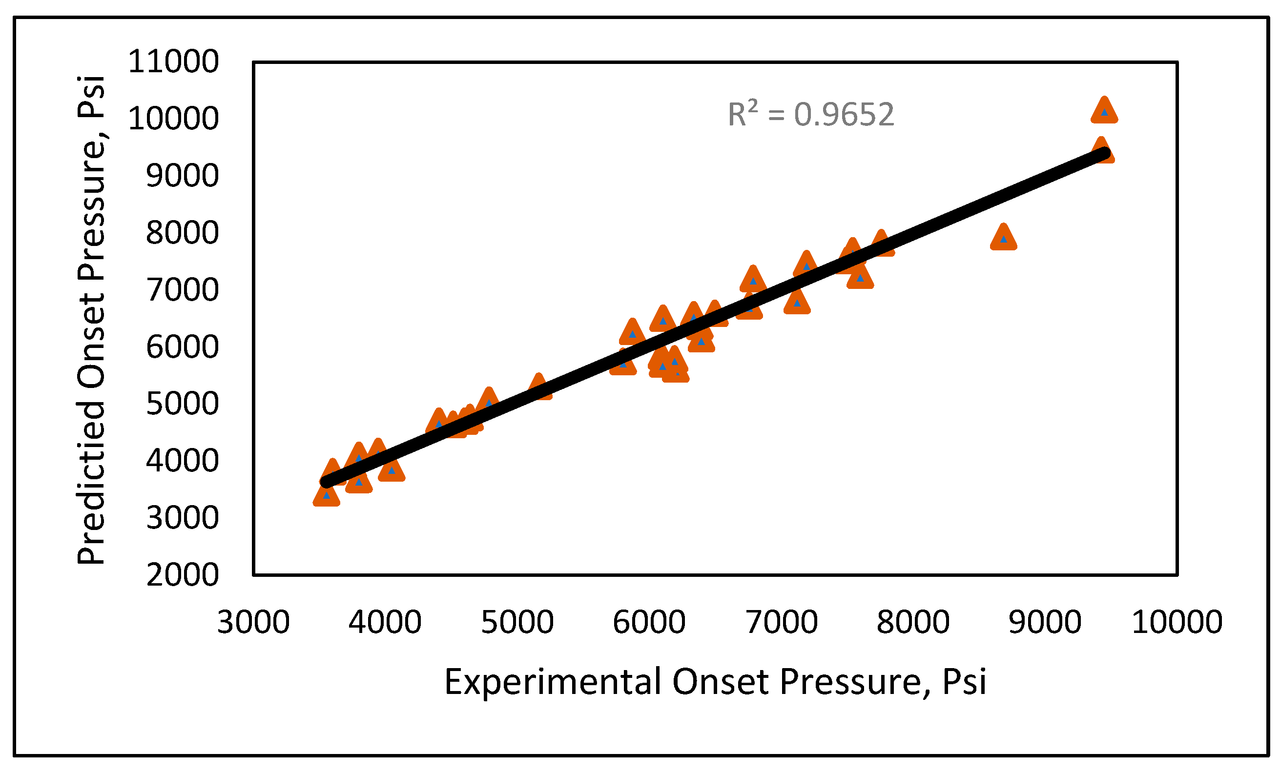
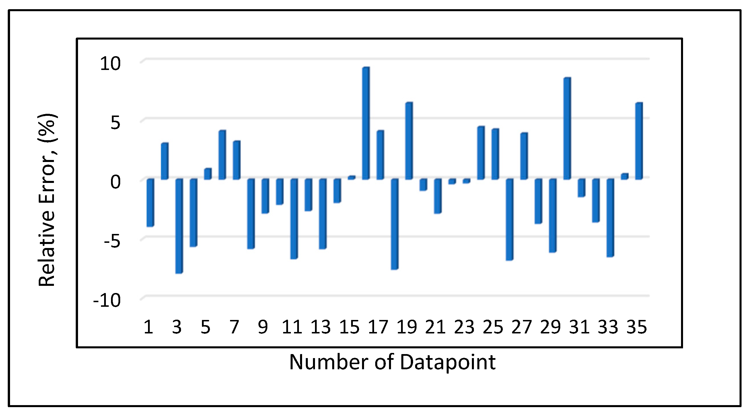
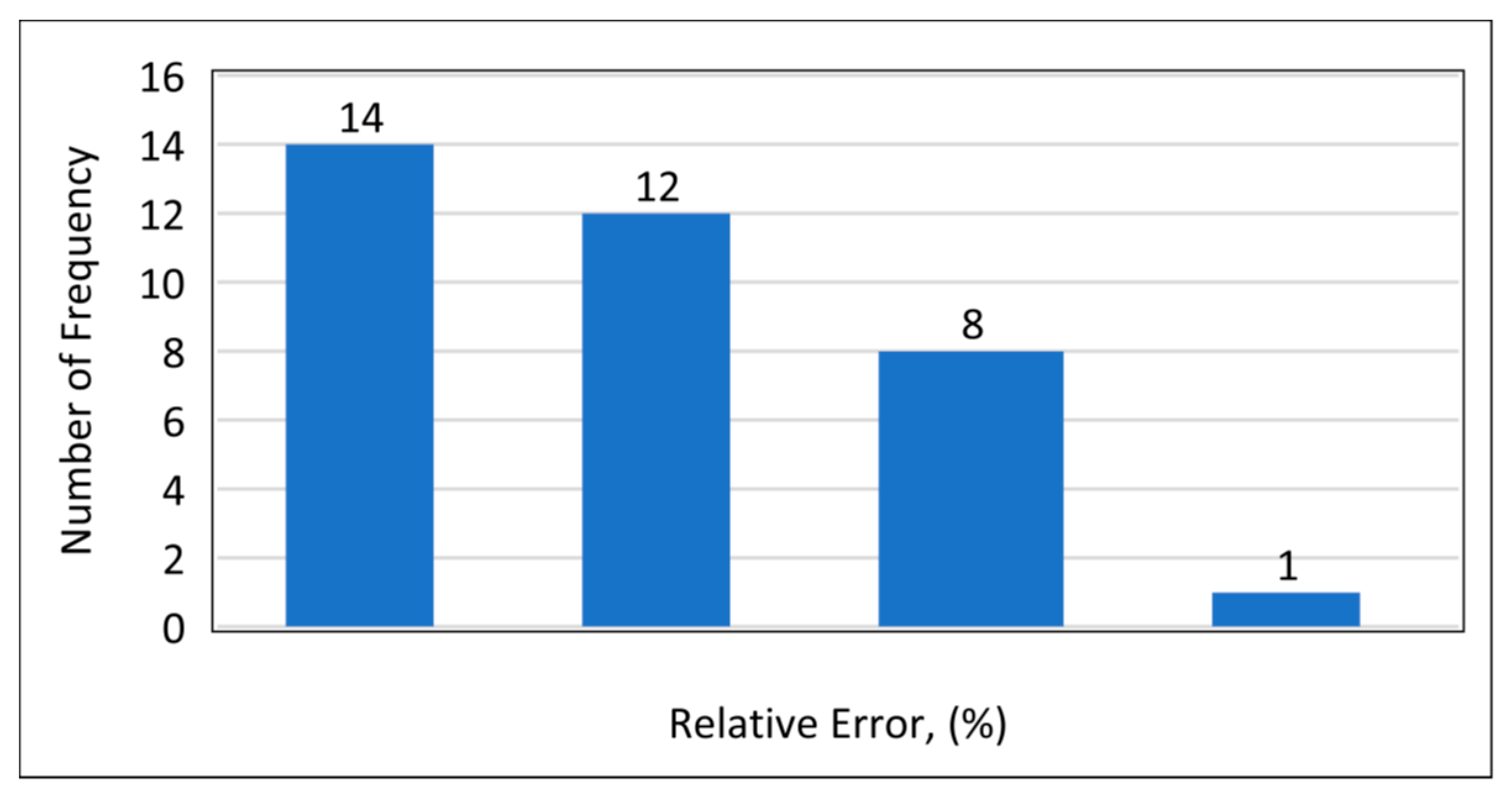
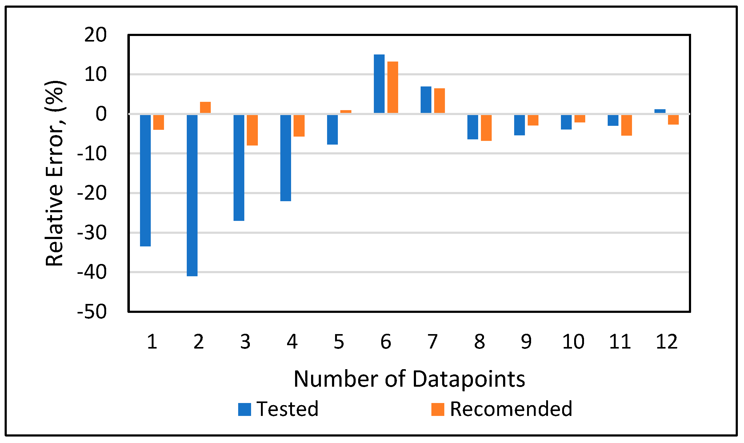
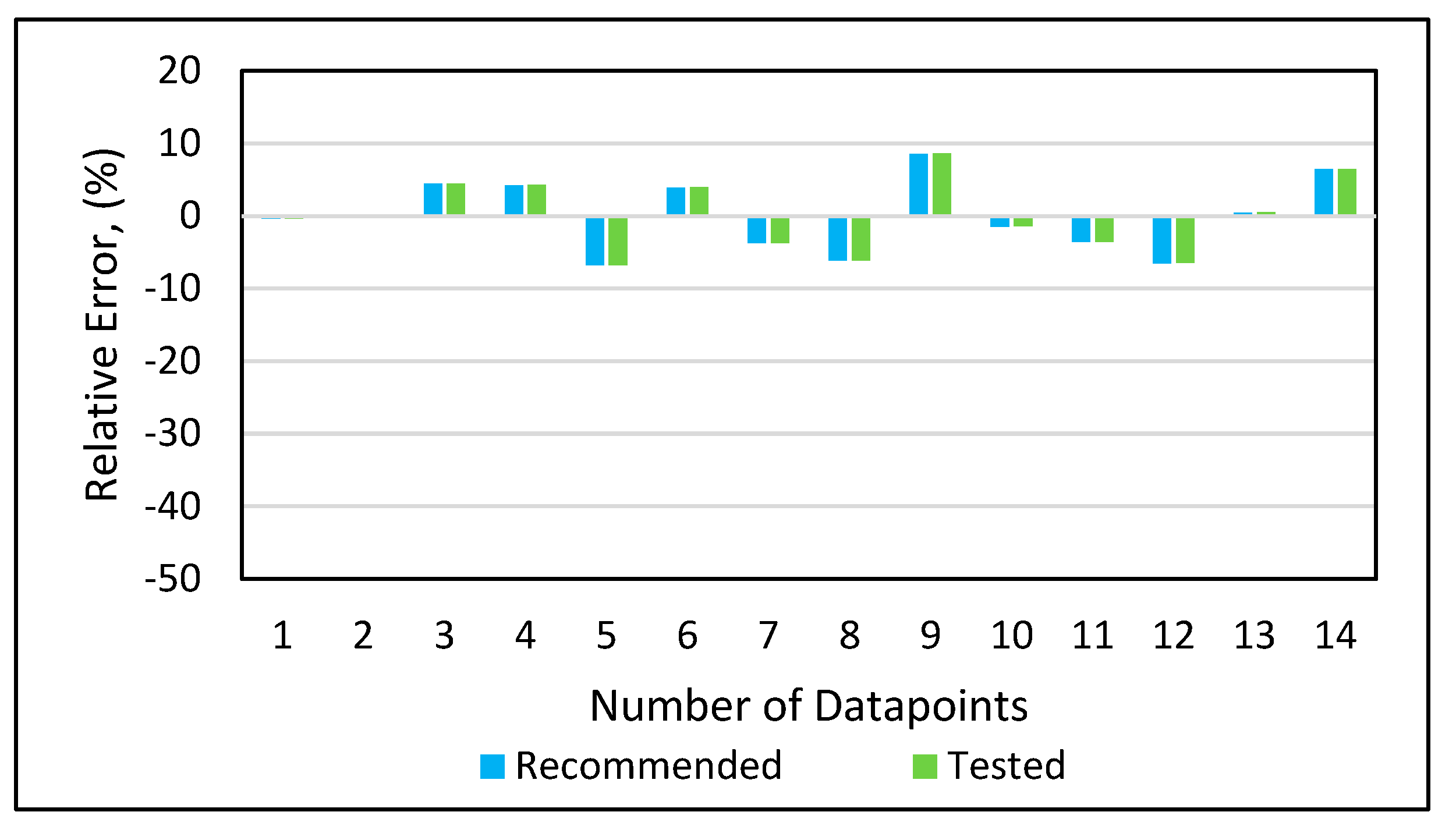
Model 1a was applied to the 12 testing data points listed in Table A3 (Appendix). Model 1b was applied to the nine testing data points give in Table A3 (Appendix), while Model 1c was applied to the 14 testing data points provided in Table A3 (Appendix). Figure 10 shows the predicted vs. experimental results for the testing data using all three models. The black line is the best fit line placed to obtain R2. The results showed that the regression performed using the provided models predicted the onset pressure with a respectable degree of accuracy, with an average R2 coefficient of 0.9652, demonstrating that the experimental and predicted results are in good agreement. Figure 11 shows the relative error of the testing data points and indicates that by applying the developed models, the testing data set had a minimum error of 1% and maximum error of 9%. The amount of error that is acceptable depends on the experiment, but a margin of error of 10% is generally considered acceptable (Burruss and Bray , 2005). The error frequency plot given in Figure 12 shows that 14 data points had errors of less than 3%, 12 datapoints had errors between 3 and 6%, and nine data points had errors of 6-9%.
Figure 10.
Experimental vs. predicted onset pressure.
Figure 10.
Experimental vs. predicted onset pressure.
Figure 11.
Relative error analysis.
Figure 11.
Relative error analysis.
Figure 12.
Frequency of error.
Figure 12.
Frequency of error.
4. Results and Analysis
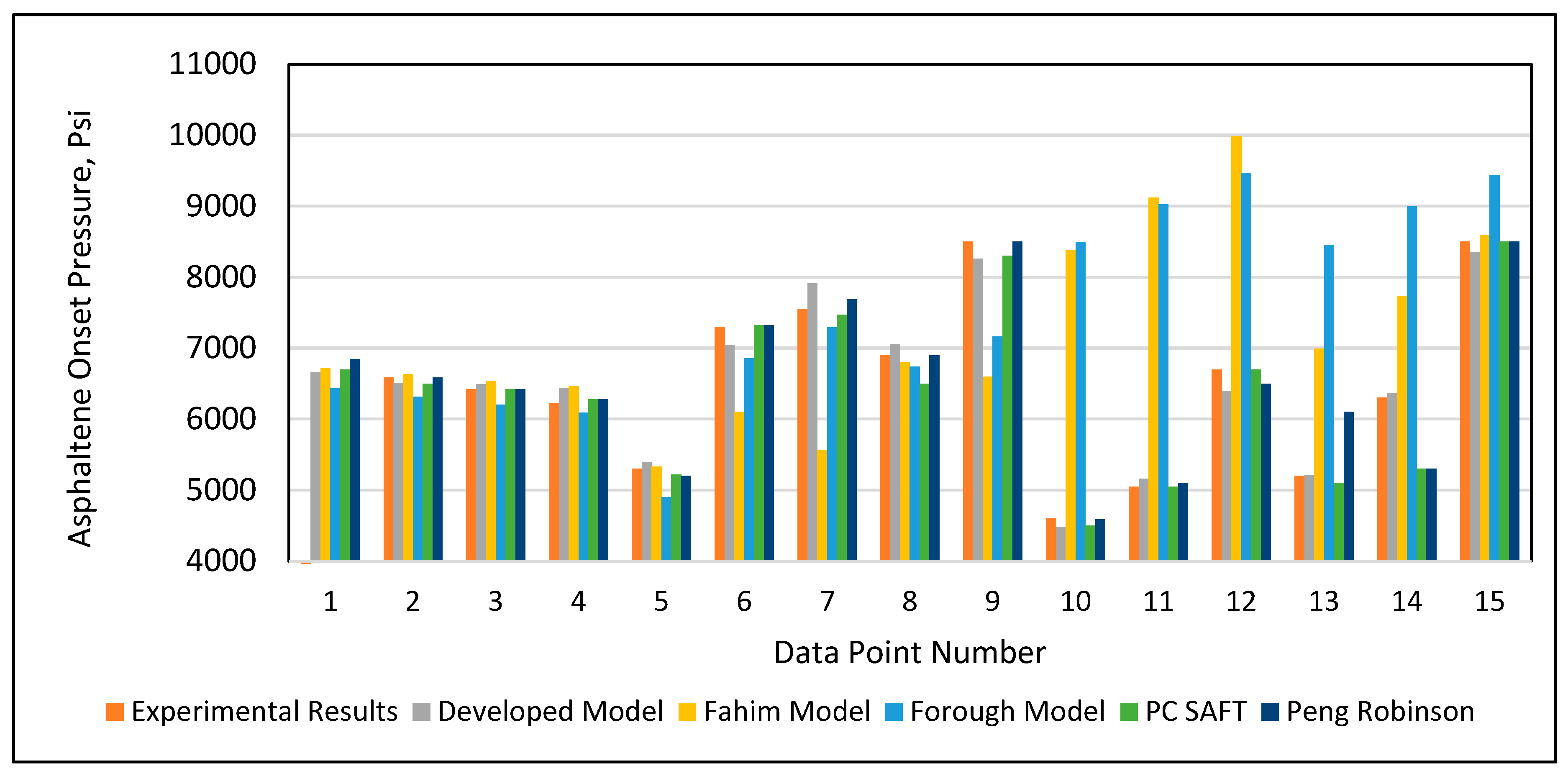
In addition to validation against the experimental data, the developed model was tested again against Fahim’s model (2007), Ameli et al.’s model (2016), the PC SAFT equation of state, and the Peng-Robinson (PR) equation of state using 15 data points selected randomly from the database given in Table A1 (Appendix). The PC SAFT and PR equations of state were applied using SARA-based live crude oil. The complete procedure to apply an equation of state is provided in Buriro et al. (2021). Table 6 and Figure 13 present the results of all of the models’ predictions of the onset pressure. The results demonstrated that Fahim’s model had an error greater than 10% error in predicting the onset pressure for the data points 1, 2, 3, 9, 12, 13, and 14, as shown in Table 6. Ameli et al.’s model likewise performed poorly in predicting the data points 1, 2, 3, 4, 5, 6, 9,12,14, and 15, as given in Table 6. After employing the tuning parameters, the PC SAFT and PR equations of state provided acceptable predictions for all onset pressure data points. Similarly, the developed model from this study made acceptable predictions for all onset pressure data points. However, in terms of performance and ease of use, our developed model outperformed the other two equation of state models.
Table 6.
Results of the predicted onset pressure of all models.
Table 6.
Results of the predicted onset pressure of all models.
| No. |
Experimental Onset Pressure (AOP) Lab Results (psi) |
Developed Model
(psi) |
Fahim’s Model
(psi) |
Ameli et al.’s Model
(psi) |
PC SAFT
(psi) |
Peng- Robinson
(psi) |
| 1.00 |
4600 |
4484 |
8382.38 |
8493.74 |
4500 |
4590 |
| 2.00 |
5050 |
5159 |
9122.88 |
9025.36 |
5050 |
5100 |
| 3.00 |
5200 |
5209 |
6992.3 |
8456.76 |
5100 |
6100 |
| 4.00 |
5299 |
5388 |
5330.7 |
4899.8 |
5221 |
5200 |
| 5.00 |
6225 |
6436 |
6470.83 |
6089.93 |
6279 |
6279.91 |
| 6.00 |
6300 |
6369 |
7732.8 |
8999.55 |
5300 |
5300 |
| 7.00 |
6419 |
6492 |
6540.14 |
6203.51 |
6419 |
6419.14 |
| 8.00 |
6587 |
6508 |
6632.47 |
6317.1 |
6500 |
6584.48 |
| 9.00 |
6700 |
6396 |
9985.46 |
9468.21 |
6700 |
6500.17 |
| 10.00 |
6854 |
6654 |
6717.04 |
6430.69 |
6700 |
6845.54 |
| 11.00 |
6900 |
7057 |
6795.75 |
6739.49 |
6500 |
6900 |
| 12.00 |
7300 |
7047 |
6102.66 |
6855.75 |
7324.15 |
7324.15 |
| 13.00 |
7550 |
7912 |
5565.8 |
7294.58 |
7469.18 |
7686.73 |
| 14.00 |
8500 |
8259 |
6598.65 |
7161.85 |
8300 |
8500 |
| 15.00 |
8500 |
8354 |
8595.38 |
9431.68 |
8500 |
8500.00 |
Figure 13.
Results of the predicted onset pressure of all models.
Figure 13.
Results of the predicted onset pressure of all models.
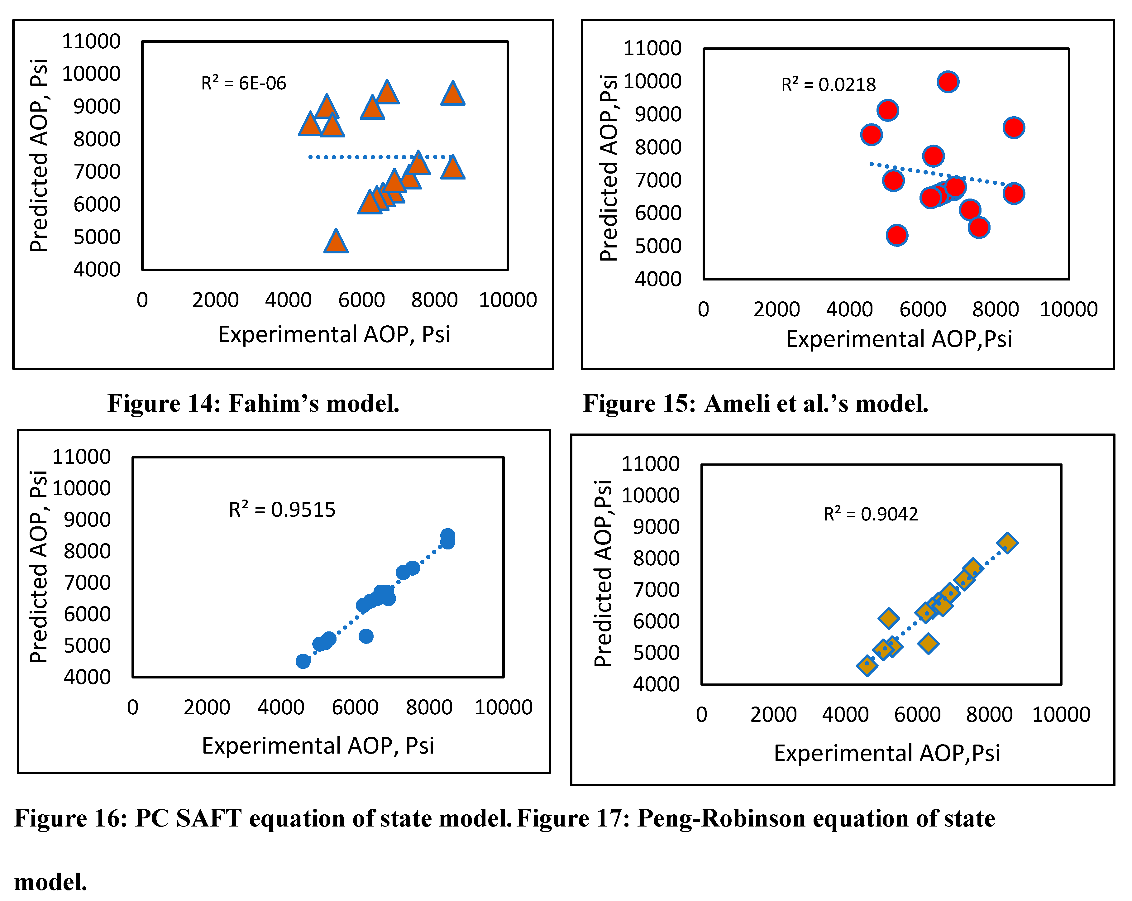
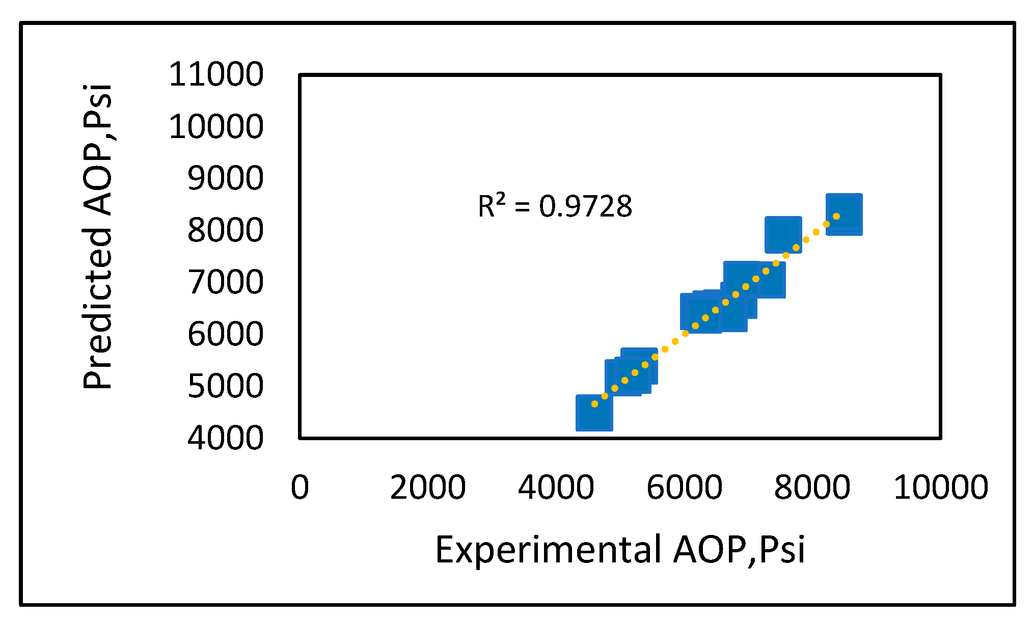
Experimental vs. predicted onset pressure plots (Figures 14-18) were created for all models, and the best fit model was drawn to obtain R2. There was not a good fitting line to connect the results for Fahim’s model (Figure 14), other than for few data points, and Ameli et al.’s model (Figure 16) was a similarly poor predictor. However, the results using the PC SAFT and Peng-Robinson equations of state (Figures 17 and 18) showed a good match with the experimental data, with R2 above 90%. The new developed model also demonstrated good prediction results (Figure 18) with an R2. of 97%. The comparison suggests that our developed model is at least as accurate as the PC SAFT equation of state. However, using our simple prediction model can overcome some of the drawbacks associated with equations of state, such as the modeling complexity due to the need for tuning of parameters that require a trial-and-error approach.

Figure 18.
Developed asphaltene onset pressure model.
Figure 18.
Developed asphaltene onset pressure model.
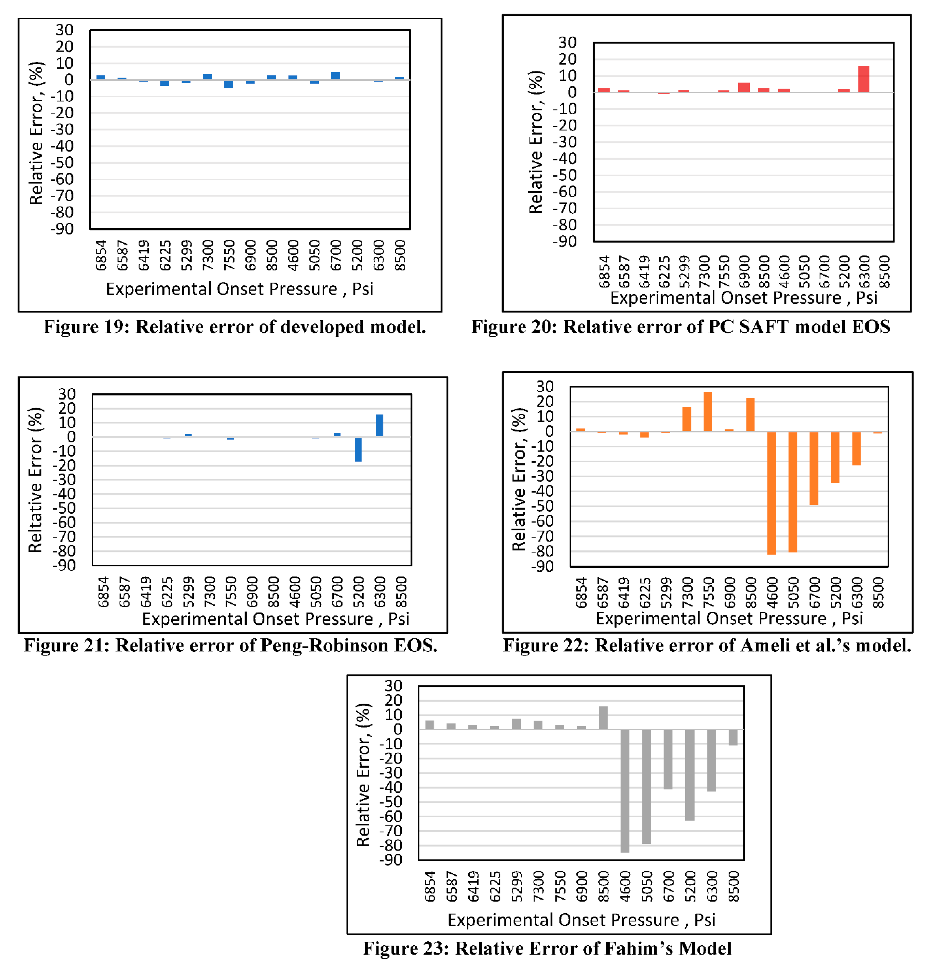
Relative error analysis was also conducted for all of the models. The new developed model (Figure 19) had a maximum error of 4.4% at an onset pressure of 7550 psi. The PC SAFT (Figure 20) produced a maximum error of 15% at an onset pressure of 6300 psi, while it had less than a 10% error at all other data points. The Peng-Robinson (Figure 21) had a maximum error or 17% at an onset pressure of 5300 psi and an error of 15% at an onset pressure of 6300 psi, while all other data points had errors less than 10%. However, significant relative errors (Figure 22 and Figure 23) were observed at various data points for both the Ameli et al. and Fahim models, with maximum errors of 82.2 and 84.6%, respectively. A margin of 10% is usually acceptable in engineering experiments (Burruss and Bray, 2005). Therefore, Fahim’s and Ameli et al.’s models cannot be used with certainty because of their higher level of relative errors.

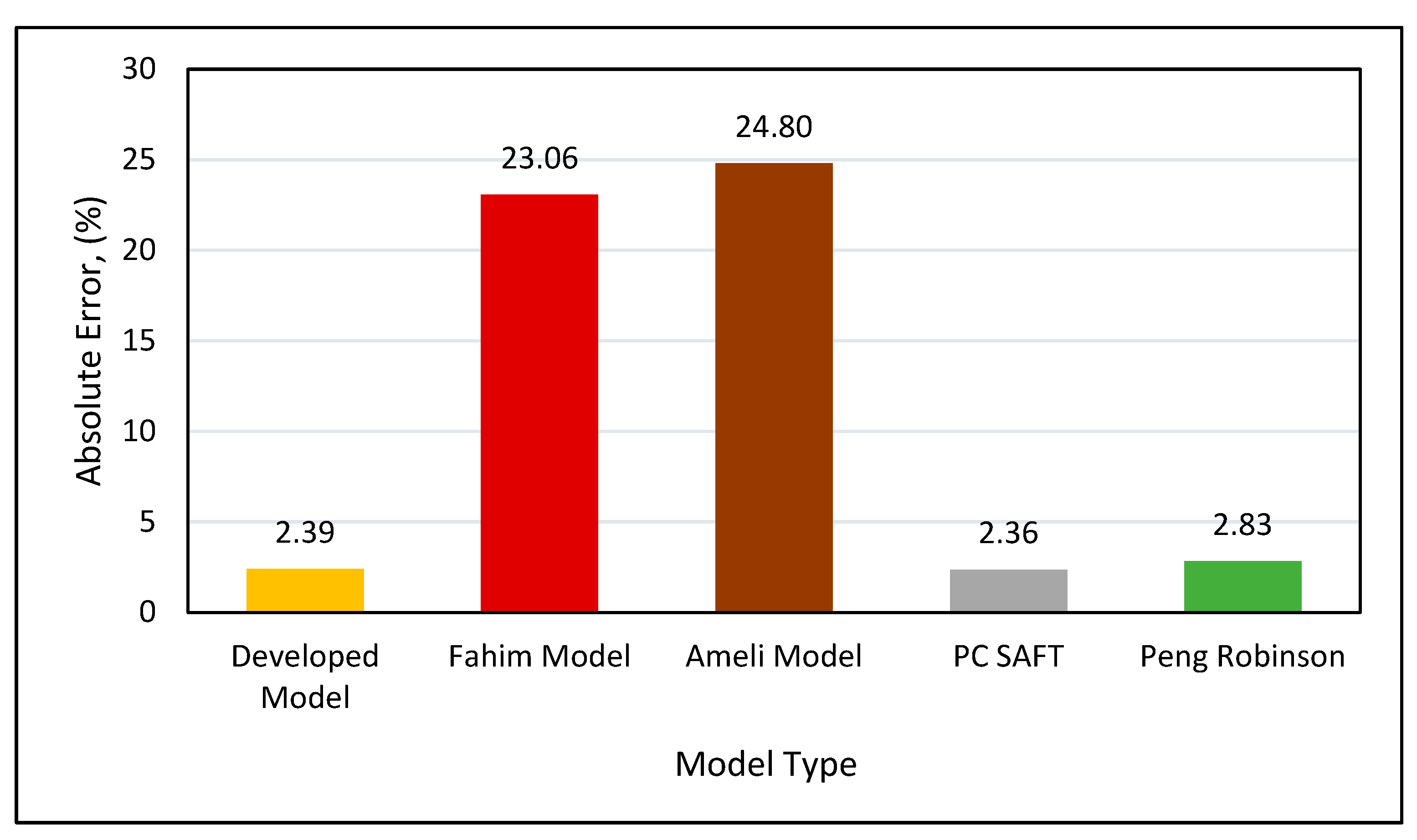
Absolute error analysis (Figure 25) indicated that the highest error of 24.7% was observed in Ameli et al.’s model, followed by 23.06% when using Fahim’s model. The Peng-Robinson had an absolute error of 2.82%, while the PC SAFT and our new developed model performed best on the tested data, with approximately a 2.35% error.
Figure 25.
Absolute error for all models.
Figure 25.
Absolute error for all models.
5. Discussion
The developed asphaltene onset pressure model has an absolute inaccuracy of 2.39 percent, as shown in Figure 25. The errors in the PR and PCSAFT equation of state models are nearly comparable, however the developed asphaltene onset pressure model outperforms the equation of state models in many ways. These benefits include shorter processing time, fewer input parameters, no experimental data adjustment, and no complication in applying approach. The developed asphaltene onset model only requires experimental onset pressure, temperature, bubble point pressure, and SARA analysis, whereas the equation of state model requires the entire crude oil composition, critical properties for all components, molecular weights for all components, experimental onset pressure, bubble point pressure, temperature, guess composition for liquid-liquid equilibria, critical properties of components, and binary interaction parameters. Obtaining several of these input characteristics may necessitate additional costs and effort. The developed onset pressure model may provide results in a matter of seconds, whereas equation of state modeling using PCSAFT takes at least 3 minutes to complete a single run and can take up to 10 minutes depending on the guess composition. To design and run the equation of state modeling algorithm, a high-performance computer and programming software are required. The equation of state model necessitates tuning using complicated experimental data that is dependent on several critical properties. According to the author's experience, tuning experimental data may take many hours depending on the composition of the oil, and it may take days to develop the whole asphaltene phase envelope for a specific oil. Our developed asphaltene onset pressure model, on the other hand, does not require substantial tuning and can generate a phase envelope in as little as 5 minutes. Equation of state modeling requires the splitting of crude oil into gas and dead oil components, which are subsequently recombined depending on SARA composition. Furthermore, it is necessary to design an advanced algorithms in a programming language to predict the onset model after tuning with experimental data, but our proposed onset pressure model is a simple and easy-to-use equation. Finally, the equation of state model necessitates technical coding skills, algorithms, and equation of state modeling, but our proposed approach necessitates no programming or computer software abilities. All of the previously mentioned factors demonstrate a clear benefit of the proposed asphaltene precipitation onset pressure model.
6. Conclusion
This study developed a direct and fast prediction model for computing the asphaltene onset pressure for reservoir pressure depletion above bubble point pressure conditions. Clustering technique was used to identify three unique groups of data. Later, multivariate regression analysis was used to develop asphaltene precipitation onset pressure model based on experimental data collected from the literature. Given the results, the following conclusions can be drawn:
Based on the onset pressure range grouping, three models were developed. The developed asphaltene precipitation onset pressure models showed excellent performance on testing data with reasonable accuracy. The PC SAFT and PR equations of state with SARA based characterization method, when used with tuning parameters, can predict the onset pressure with reasonable accuracy.
Fahim’s and Ameli et al.’s models showed very high errors in predicting the onset pressure compared to the results obtained from our newly developed asphaltene precipitation onset pressure models.
Data analysis showed asphaltene onset pressure changed with changes in the temperature and bubble point pressure. The bubble point pressure had the highest linear correlation with the asphaltene onset pressure, while temperature had a curvilinear correlation with the onset pressure, therefore higher orders of parameters in model development may provide better fitting of data.
The developed asphaltene precipitation onset pressure models can produce accurate results in a short amount of time as compared to PCSAFT and PR equation of state models that required time consuming tuning.
7. Future Work Recommendations
The currently developed asphaltene precipitation onset pressure model is limited to upper precipitation onset pressure (liquid and asphaltene envelop) and it cannot predict the lower onset pressure and onset pressure under gas injection conditions. Therefore, more work is required to develop another model that can predict lower asphaltene onset pressure and onset pressure under gas injection conditions. More work is needed to combine all of these models into a single model.
8. Nomenclature
AOP= Asphaltene Onset Pressure, Psi
Pb = Bubble Point Pressure, Psi
R = resins
A = Asphaltenes
S/A= Saturate to Aromatic Ratio
T = Temperature, oF
= Relative Error
DF= Degrees of Freedom
Adj SS= Adjusted sum of squares
S= standard deviation of the distance between the data values and the fitted values
9. Data Availability
Training and Testing data used in this work is available at the following link to download publicly.
Appendix
Table A1.
Model Comparison.
Table A1.
Model Comparison.
| No. |
Experimental
Results |
Fahim Model |
Fahim's Model Error |
Ameli’s Model |
Ameli’s Model error |
| 1.00 |
6854.00 |
6717.04 |
2.00 |
6430.69 |
3.36 |
| 2.00 |
6587.00 |
6632.47 |
-0.69 |
6317.10 |
2.93 |
| 3.00 |
6419.00 |
6540.14 |
-1.89 |
6203.51 |
4.44 |
| 4.00 |
6225.00 |
6470.83 |
-3.95 |
6089.93 |
5.38 |
| 5.00 |
5299.00 |
5330.70 |
-0.60 |
4899.80 |
9.06 |
| 6.00 |
7300.00 |
6102.66 |
16.40 |
6855.75 |
2.71 |
| 7.00 |
7550.00 |
5565.80 |
26.28 |
7294.58 |
7.80 |
| 8.00 |
6900.00 |
6795.75 |
1.51 |
6739.49 |
4.50 |
| 9.00 |
8500.00 |
6598.65 |
22.37 |
7161.85 |
13.28 |
| 10.0 |
4600.00 |
8382.38 |
-82.23 |
8493.74 |
-89.42 |
| 11.0 |
5050.00 |
9122.88 |
-80.65 |
9025.36 |
-74.94 |
| 12.0 |
6700.00 |
9985.46 |
-49.04 |
9468.21 |
-48.03 |
| 13.0 |
5200.00 |
6992.30 |
-34.47 |
8456.76 |
-62.35 |
| 14.0 |
6300.00 |
7732.80 |
-22.74 |
8999.55 |
-41.30 |
| 15.00 |
8500.00 |
8595.38 |
-1.12 |
9431.68 |
-12.90 |
Table A2.
Experimental Data Collection for Model Training.
Table A2.
Experimental Data Collection for Model Training.
| No. |
Oil Name |
Saturates (%) |
Aromatics
(%) |
Resins
(%) |
Asphaltene
(%) |
Temperature (F) |
Bubble Point Pressure (Psi) |
Onset Pressure
(Psi) |
Data
Reference |
| 1 |
Oil X-1 |
68.3 |
11.6 |
18.8 |
3.5 |
210.2 |
3221 |
6854 |
Jamaluddin et al,2002 |
| 2 |
Oil X-1 |
68.3 |
11.6 |
18.8 |
3.5 |
219.2 |
3283 |
6587 |
| 3 |
Oil X-1 |
68.3 |
11.6 |
18.8 |
3.5 |
230 |
3276 |
6419 |
| 4 |
Oil X-1 |
68.3 |
11.6 |
18.8 |
3.5 |
240 |
3289 |
6225 |
| 5 |
Oil X-2 |
65.6 |
16.3 |
13.5 |
4.6 |
212 |
4259 |
5299 |
Jamaluddin et al,2002 |
| 6 |
Oil X-3 |
70.88 |
24.21 |
3.87 |
1.04 |
289 |
4283 |
7300 |
Hassanvand et al, 2012 |
| 7 |
Oil X-3 |
70.88 |
24.21 |
3.87 |
1.04 |
240 |
4150 |
7550 |
| 8 |
Oil X-4 |
74.81 |
21.59 |
2.63 |
0.97 |
289 |
4843 |
6900 |
Hassanvand et al, 2012 |
| 9 |
Oil X-4 |
74.81 |
21.59 |
2.63 |
0.97 |
248 |
4617 |
8500 |
| 10 |
Oil X-5 |
39.2 |
35.9 |
9.0 |
15.5 |
208 |
2420 |
4600 |
Gonzalez et al, 2005 |
| 11 |
Oil X-5 |
39.2 |
35.9 |
9.0 |
15.5 |
150 |
2128 |
5050 |
| 12 |
Oil X-5 |
39.2 |
35.9 |
9.0 |
15.5 |
100 |
1850 |
6700 |
| 13 |
Oil X-6 |
57.5 |
30.4 |
8.3 |
3.7 |
208 |
3617 |
5200 |
Gonzalez et al, 2005 |
| 14 |
Oil X-6 |
57.5 |
30.4 |
8.3 |
3.7 |
150 |
3460 |
5300 |
| 15 |
Oil X-6 |
57.5 |
30.4 |
8.3 |
3.7 |
100 |
3565 |
8500 |
| 16 |
Oil X-7 |
53 |
28.1 |
13.9 |
1.4 |
271 |
2902 |
4500 |
Gonzalez et al, 2012 |
| 17 |
Oil X-7 |
53 |
28.1 |
13.9 |
1.4 |
182 |
2568 |
4200 |
| 18 |
Oil X-7 |
53 |
28.1 |
13.9 |
1.4 |
94 |
1922 |
3700 |
| 19 |
Oil X-8 |
54.67 |
28.89 |
12.66 |
3.8 |
284 |
2692 |
5005 |
Buenrostro-Gonzalez et al, 2004 |
| 20 |
Oil X-8 |
54.67 |
28.89 |
12.66 |
3.8 |
248 |
2480 |
5228 |
| 21 |
Oil X-8 |
54.67 |
28.89 |
12.66 |
3.8 |
194 |
2377 |
5511 |
| 22 |
Oil X-8 |
54.67 |
28.89 |
12.66 |
3.8 |
178 |
NA |
na |
| 23 |
Oil X-8 |
54.67 |
28.89 |
12.66 |
3.8 |
167 |
2027 |
5600 |
| 24 |
Oil X-8 |
54.67 |
28.89 |
12.66 |
3.8 |
144 |
NA |
Na |
| 25 |
Oil X-9 |
55.14 |
30.73 |
10.88 |
3.25 |
284 |
2940 |
5398 |
Buenrostro-Gonzalez et al, 2004 |
| 26 |
Oil X-9 |
55.14 |
30.73 |
10.88 |
3.25 |
248 |
2850 |
6607 |
| 27 |
Oil X-9 |
55.14 |
30.73 |
10.88 |
3.25 |
194 |
NA |
na |
| 28 |
Oil X-9 |
55.14 |
30.73 |
10.88 |
3.25 |
178 |
2620 |
6874 |
| 29 |
Oil X-9 |
55.14 |
30.73 |
10.88 |
3.25 |
167 |
NA |
Na |
| 30 |
Oil X-9 |
55.14 |
30.73 |
10.88 |
3.25 |
144 |
2435 |
8705 |
| 31 |
Oil X-10 |
75.3 |
20 |
4.4 |
0.3 |
275 |
3720 |
4967 |
Behnam, and Zare-Reisabadi, 2015 |
| 32 |
Oil X-10 |
75.3 |
20 |
4.4 |
0.3 |
235 |
3583 |
5143 |
| 33 |
Oil X-10 |
75.3 |
20 |
4.4 |
0.3 |
194 |
3413 |
5555 |
| 34 |
Oil X-10 |
75.3 |
20 |
4.4 |
0.3 |
155 |
3223 |
6060 |
| 35 |
Oil X-10 |
75.3 |
20 |
4.4 |
0.3 |
115 |
3007 |
6739 |
| 36 |
Oil X-11 |
54.19 |
37.96 |
6.48 |
1.37 |
240 |
3150 |
4500 |
Abutaqiya et al, 2021 |
| 37 |
Oil X-11 |
54.19 |
37.96 |
6.48 |
1.37 |
180 |
|
|
| 38 |
Oil X-11 |
54.19 |
37.96 |
6.48 |
1.37 |
110 |
|
|
| 39 |
Oil X-12 |
49.47 |
46.98 |
2.82 |
0.74 |
230 |
3175 |
4923 |
Abutaqiya et al, 2021 |
| 40 |
Oil X-12 |
49.47 |
46.98 |
2.82 |
0.74 |
180 |
2900 |
5515 |
| 41 |
Oil X-12 |
49.47 |
46.98 |
2.82 |
0.74 |
110 |
2529 |
7000 |
| 42 |
Oil X-13 |
47.42 |
47.81 |
3.88 |
0.88 |
229 |
3164 |
4805 |
Abutaqiya et al, 2021 |
| 43 |
Oil X-13 |
47.42 |
47.81 |
3.88 |
0.88 |
180 |
2877 |
4900 |
| 44 |
Oil X-13 |
47.42 |
47.81 |
3.88 |
0.88 |
110 |
2420 |
6592 |
| 45 |
Oil X-14 |
48.36 |
44.34 |
6.27 |
1.03 |
243 |
2312 |
4300 |
Abutaqiya et al, 2021 |
| 46 |
Oil X-14 |
48.36 |
44.34 |
6.27 |
1.03 |
185 |
2086 |
4600 |
| 47 |
Oil X-14 |
48.36 |
44.34 |
6.27 |
1.03 |
138 |
1800 |
4805 |
| 48 |
Oil X-15 |
66.6 |
27 |
5.3 |
0.2 |
167 |
2700 |
8000 |
Sullivan et al, 2020 |
| 49 |
Oil X-15 |
66.6 |
27 |
5.3 |
0.2 |
212 |
2900 |
7000 |
| 50 |
Oil X-15 |
66.6 |
27 |
5.3 |
0.2 |
257 |
3100 |
5500 |
| 51 |
Oil X-16 |
70.6 |
22.5 |
2.5 |
2.5 |
167 |
2950 |
8750 |
Sullivan et al, 2020 |
| 52 |
Oil X-16 |
70.6 |
22.5 |
2.5 |
2.5 |
212 |
3100 |
6750 |
| 53 |
Oil X-16 |
70.6 |
22.5 |
2.5 |
2.5 |
257 |
3200 |
5750 |
| 54 |
Oil X-17 |
69.49 |
21.84 |
8.89 |
0.36 |
237 |
3160 |
5713 |
Al-Obaidli., et al, 2019 |
| 55 |
Oil X-17 |
69.49 |
21.84 |
8.89 |
0.36 |
159 |
NA |
7538 |
| 56 |
Oil X-17 |
69.49 |
21.84 |
8.89 |
0.36 |
|
|
|
| 57 |
Oil X-18 |
70.61 |
20.22 |
8.46 |
0.45 |
237 |
3035 |
5612 |
Al-Obaidli,et al, 2019 |
| 58 |
Oil X-18 |
70.61 |
20.22 |
8.46 |
0.45 |
159 |
NA |
7671 |
| 59 |
Oil X-18 |
70.61 |
20.22 |
8.46 |
0.45 |
|
|
|
Table A3.
Experimental Data Collection for Model Testing.
Table A3.
Experimental Data Collection for Model Testing.
| No. |
Resin |
SA |
Temp |
Pb |
Experimental AOP |
Data Reference |
| Model1a: Testing Dataset |
|
| 1. |
1.05 |
3.4 |
254.93 |
2300 |
3755.5 |
Fahim (2007) |
| 2. |
1.53 |
0.98 |
244.13 |
1900 |
3552.5 |
Fahim (2007) |
| 3. |
2.1 |
3 |
230 |
2400 |
3799 |
Fahim (2007) |
| 4. |
2.3 |
1 |
236 |
2500 |
3944 |
Fahim (2007) |
| 5. |
7.6 |
2.4 |
190.13 |
4263 |
5800 |
Fahim (2007) |
| 6. |
10.4 |
1.8 |
190 |
2500 |
5400 |
Jamaluddin et al, 2002 |
| 7. |
10.4 |
1.8 |
230 |
2700 |
4050 |
Jamaluddin et al, 2002 |
| 8. |
10.4 |
1.8 |
260 |
2900 |
3650 |
Jamaluddin et al, 2002) |
| 9. |
4.08 |
1.17 |
240 |
3059 |
4513 |
Al-Obaidli, et al, 2019 |
| 10. |
4.08 |
1.17 |
230 |
3060 |
4600 |
Al-Obaidli, et al, 2019 |
| 11. |
8.32 |
2.452 |
240 |
3064 |
4405 |
Al-Obaidli, et al, 2019 |
| 12. |
8.32 |
2.452 |
230 |
3150 |
4640 |
Al-Obaidli, et al, 2019 |
| Model1b : Testing Dataset |
|
| 13. |
6.4 |
1.48 |
130.73 |
3480 |
4785 |
Fahim (2007) |
| 14. |
7 |
1.8 |
103.73 |
3220 |
7541 |
Fahim (2005) |
| 15. |
7 |
1.8 |
177.53 |
3277 |
6381 |
Fahim (2005) |
| 16. |
7 |
1.8 |
240.53 |
3350 |
6200 |
Fahim (2005) |
| 17. |
7 |
1.8 |
286 |
3250 |
6091 |
Fahim (2005) |
| 18. |
7.3 |
3.1 |
120 |
2552 |
9450 |
Fahim (2005) |
| 19. |
7.4 |
1.7 |
231.53 |
3161 |
6190 |
Fahim (2005) |
| 20. |
11.3 |
3.5 |
150.53 |
2856.5 |
7757.5 |
Fahim (2005) |
| 21. |
13 |
3 |
211.73 |
2914.5 |
5162 |
Al-Obaidli, et al, 2019 |
| Model1c: Testing Dataset |
|
| 22. |
4.6 |
3.9 |
235.13 |
3973 |
9425 |
Fahim (2005) |
| 23. |
6 |
1.8 |
246.11 |
3016 |
7496.5 |
Al-Obaidli, et al, 2019 |
| 24. |
7.9 |
2.9 |
238.73 |
3451 |
7598 |
Al-Obaidli, et al, 2019 |
| 25. |
11.3 |
3.5 |
240.53 |
3248 |
7119.5 |
Fahim (2007) |
| 26. |
11.3 |
3.5 |
305.33 |
3393 |
5872.5 |
Fahim (2007) |
| 27. |
11.3 |
3.5 |
319.19 |
3422 |
6394.5 |
Fahim (2007) |
| 28. |
11.3 |
3.5 |
179.33 |
2958 |
7192 |
Fahim (2007) |
| 29. |
11.3 |
3.5 |
209.93 |
3088.5 |
6786 |
Fahim (2005) |
| 30. |
11.3 |
3.5 |
119.93 |
2552 |
8685.5 |
Fahim (2005) |
| 31. |
18.8 |
5.88 |
218.93 |
3233.5 |
6496 |
Fahim (2005) |
| 32. |
18.8 |
5.88 |
229.73 |
3233.5 |
6336.5 |
Fahim (2005) |
| 33. |
18.8 |
5.88 |
242.33 |
3248 |
6104.5 |
Fahim (2005) |
| 34. |
18.8 |
5.88 |
209.93 |
3175.5 |
6757 |
Fahim (2005) |
| 35 |
7.59 |
1.138 |
224 |
3064 |
6100 |
Fahim (2005) |
Table A4.
Model1a Subset Analysis.
Table A4.
Model1a Subset Analysis.
| No. |
R-Sq |
R-Sq (adj) |
R-Sq (pred) |
Mallows Cp |
S |
R |
S/A |
T, OF |
Pb
|
T2
|
Pb2
|
Pb*t |
| 1 |
71.0 |
69.3 |
60.9 |
110.8 |
577.80 |
|
|
X |
|
|
|
|
| 2 |
62.9 |
60.7 |
48.8 |
145.6 |
652.91 |
|
|
|
|
X |
|
|
| 3 |
85.7 |
83.9 |
75.0 |
49.1 |
418.39 |
|
|
X |
X |
|
|
|
| 4 |
85.3 |
83.4 |
73.6 |
50.9 |
424.44 |
|
|
X |
|
|
|
X |
| 5 |
95.2 |
94.2 |
90.8 |
9.8 |
250.30 |
|
|
X |
X |
X |
|
|
| 6 |
93.9 |
92.7 |
87.4 |
15.2 |
280.82 |
|
|
X |
|
X |
X |
|
| 7 |
96.7 |
95.7 |
93.2 |
5.4 |
215.14 |
|
|
X |
X |
X |
|
X |
| 8 |
96.1 |
95.0 |
90.5 |
7.9 |
233.25 |
|
|
X |
X |
X |
X |
|
| 9 |
97.3 |
96.3 |
91.3 |
4.6 |
200.39 |
X |
|
X |
|
X |
X |
X |
| 10 |
96.9 |
95.7 |
90.0 |
6.4 |
215.93 |
X |
|
X |
X |
X |
|
X |
| 11 |
97.4 |
96.2 |
87.7 |
6.1 |
203.85 |
X |
|
X |
X |
X |
X |
X |
| 12 |
97.3 |
96.0 |
90.1 |
6.5 |
208.23 |
X |
X |
X |
|
X |
X |
X |
| 13 |
97.5 |
95.8 |
86.3 |
8.0 |
212.41 |
X |
X |
X |
X |
X |
X |
X |
Table A5.
Model1b Subset Analysis.
Table A5.
Model1b Subset Analysis.
| No. |
R-Sq |
R-Sq (adj) |
R-Sq (pred) |
Mallows Cp |
S |
R |
S/A |
T, OF |
Pb
|
T2
|
Pb2
|
Pb*t |
| 1 |
71.1 |
68.4 |
62.0 |
65.3 |
922.56 |
|
|
X |
|
|
|
|
| 2 |
68.7 |
65.9 |
58.2 |
71.3 |
958.69 |
|
|
|
|
X |
|
|
| 3 |
91.7 |
90.1 |
86.0 |
14.2 |
516.81 |
|
|
X |
|
|
|
X |
| 4 |
90.1 |
88.1 |
82.9 |
18.5 |
566.67 |
X |
|
X |
|
|
|
|
| 5 |
95.3 |
93.7 |
89.3 |
7.2 |
412.59 |
X |
|
X |
|
|
|
X |
| 6 |
94.2 |
92.3 |
87.5 |
9.8 |
455.38 |
X |
|
X |
X |
|
|
|
| 7 |
97.2 |
95.8 |
91.9 |
4.2 |
336.61 |
X |
|
X |
|
|
X |
X |
| 8 |
97.2 |
95.8 |
91.7 |
4.2 |
337.13 |
X |
|
X |
|
X |
|
X |
| 9 |
98.0 |
96.6 |
92.2 |
4.1 |
304.15 |
X |
|
X |
X |
|
X |
X |
| 10 |
97.8 |
96.1 |
90.9 |
4.8 |
322.40 |
X |
|
X |
|
X |
X |
X |
| 11 |
98.0 |
96.1 |
86.9 |
6.0 |
324.44 |
X |
|
X |
X |
X |
X |
X |
| 12 |
98.0 |
96.0 |
89.5 |
6.1 |
328.14 |
X |
X |
X |
X |
|
X |
X |
| 13 |
98.1 |
95.3 |
82.8 |
8.0 |
354.87 |
X |
X |
X |
X |
X |
X |
X |
Table A6.
Model1c Subset Analysis.
Table A6.
Model1c Subset Analysis.
| No. |
R-Sq |
R-Sq (adj) |
R-Sq (pred) |
Mallows Cp |
S |
R |
S/A |
T, OF |
Pb
|
T2
|
Pb2
|
Pb*t |
| 1 |
63.3 |
60.4 |
50.3 |
133.1 |
844.22 |
|
|
|
X |
|
|
|
| 2 |
62.7 |
59.8 |
46.6 |
135.4 |
851.06 |
|
|
|
|
|
X |
|
| 3 |
85.0 |
82.5 |
75.7 |
49.8 |
561.17 |
X |
X |
|
|
|
|
|
| 4 |
73.2 |
68.7 |
56.9 |
96.3 |
751.15 |
|
|
|
X |
|
|
X |
| 5 |
94.9 |
93.5 |
90.2 |
13.1 |
342.82 |
X |
X |
|
|
|
X |
|
| 6 |
92.2 |
90.1 |
84.3 |
23.6 |
422.82 |
X |
X |
|
X |
|
|
|
| 7 |
98.2 |
97.5 |
96.2 |
2.0 |
212.66 |
X |
X |
X |
|
|
|
X |
| 8 |
96.0 |
94.5 |
90.4 |
10.5 |
316.15 |
X |
X |
|
|
X |
|
X |
| 9 |
98.2 |
97.2 |
95.3 |
4.0 |
223.68 |
X |
X |
X |
|
X |
|
X |
| 10 |
98.2 |
97.2 |
93.7 |
4.0 |
223.84 |
X |
X |
X |
|
|
X |
X |
| 11 |
98.2 |
96.9 |
90.1 |
6.0 |
237.23 |
X |
X |
X |
|
X |
X |
X |
| 12 |
98.2 |
96.9 |
91.2 |
6.0 |
237.25 |
X |
X |
X |
X |
X |
|
X |
| 13 |
98.2 |
96.4 |
81.4 |
8.0 |
253.60 |
X |
X |
X |
X |
X |
X |
X |
Figure A1.
Subset Equation based on
Table A4 No.9.
Figure A1.
Subset Equation based on
Table A4 No.9.
Figure A2.
Subset Equation based on
Table A5 No.11.
Figure A2.
Subset Equation based on
Table A5 No.11.
Figure A3.
Subset Equation based on
Table A6 No.12.
Figure A3.
Subset Equation based on
Table A6 No.12.
References
- Alhosani A., Daraboina N., (2020). Modeling of asphaltene deposition during oil/gas flow in wellbore, Fuel, Volume 280,118617. [CrossRef]
- Al-Obaidli, A., Al-Nasheet, A., Snasiri, F., Al-Shammari, O., Al-Shammari, A., Sinha, S., Muhammad Amjad, Y., Gonzalez, D., & Gonzalez, F. (2019, 18–21, 2019 ). Understanding reservoir fluid behavior to mitigate risk associated to asphaltene deposition in the reservoir rock near to asphaltene onset pressure AOP in the Magwa Marrat depleted reservoir [Paper presentation]. SPE Middle East Oil and Gas Show and Conference, Manama, Bahrain. [CrossRef]
- Ameli, F., Hemmati-Sarapardeh, A., Dabir, B, Mohammadi, A (2016). Determination of asphaltene precipitation conditions during natural depletion of oil reservoirs: A robust compositional approach, Fluid Phase Equilibria 412, 235-248. [CrossRef]
- Abutaqiya, M. I. L., Caleb J. Sisco, Khemka Y, Muhieddine A. Safa, Ebtisam F. Ghloum, Abeer M. Rashed, Ridha Gharbi, Sriram Santhanagopalan, Misfera Al-Qahtani, Eman Al-Kandari, and Francisco M. Vargas, Accurate Modeling of Asphaltene Onset Pressure in Crude Oils Under Gas Injection Using Peng–Robinson Equation of State, Energy & Fuels 2020 34 (4), 4055-4070. [CrossRef]
- Buenrostro-Gonzalez, E., Lira-Galeana, C., Gil-Villegas, A. & Wu, J. (2004), Asphaltene precipitation in crude oils: Theory and experiments. AIChE Journal, 50, 2552-2570. [CrossRef]
- Buriro, M.&Talib Shuker, M.. (2012, December 3-5). Asphaltene prediction and prevention: A strategy to control asphaltene precipitation [Paper presentation].SPE/PAPG Annual Technical Conference, Islamabad, Pakistan.
- Buriro, M.&Talib Shuker, M. (2013, May 19-22). Minimizing asphaltene precipitation in Malaysian reservoir [Paper presentation]. SPE Saudi Arabia Section Technical Symposium and Exhibition, Al-Khobar, Saudi Arabia. [CrossRef]
- Burruss G.W, Bray T.M.(2005), Confidence Intervals, Encyclopedia of Social Measurement, Elsevier, Pages 455-462. [CrossRef]
- Behnam M, Zare-Reisabadi M. (2015). Experimental study of temperature effect on onset pressure of asphaltene in live oil. Petroleum & Coal 57(4), 346-352.
- Chukwuemeka A. N, Onyekachukwu K. E, Alfreda O. N (2017), Assessment of aromatics to saturate ratios in three Niger Delta crudes, Egyptian Journal of Petroleum, Volume 26, Issue 3, Pages 787-790. [CrossRef]
- Dormann, C.F., Elith, J., Bacher, S., Buchmann, C., Carl, G., Carré, G., Marquéz, J.R.G., Gruber, B., Lafourcade, B., Leitão, P.J., Münkemüller, T., McClean, C., Osborne, P.E., Reineking, B., Schröder, B., Skidmore, A.K., Zurell, D. and Lautenbach, S. (2013). Collinearity: A review of methods to deal with it and a simulation study evaluating their performance. Ecography 36, 27-46.
- Enayat S., Babu N.R., Kuang J., Rezaee S., Lu H., Tavakkoli M., Wang J, Vargas F.M., (2020).On the development of experimental methods to determine the rates of asphaltene precipitation, aggregation, and deposition, Fuel, Volume 260, 116250. [CrossRef]
- Fahim M (2007). Empirical equations for estimating ADE of crude oils. Petroleum Science and Technology 25(7), 949-965.
- Fahim, M. (2005, March). Tunning EOS using molecular themodynamics to construct ashaltene deposition envelope (ADE) [Paper presentation]. SPE Middle East Oil and Gas Show and Conference, Kingdom of Bahrain.
- Gross, J. & Sadowski, G. (2001). Perturbed-chain SAFT: An equation of state based on a perturbation theory for chain molecules. Industrial & Engineering Chemistry Research 40 (4), 1244-1260.
- Gonzalez, D., Garcia, M., & Diaz, O. (2012). (2012. April **). Unusual asphaltene phase behavior of fluids from Lake Maracaibo, Venezuela [Paper presentation]. SPE Latin America and Caribbean Petroleum Engineering Conference, Mexico City, Mexico. [CrossRef]
- Gonzalez, D., Ting, P., Hirasaki, G. & Chapman, W. (2005). Prediction of asphaltene instability under gas injection with the PC-SAFT equation of state. Energy & Fuels, 19 (4), 1230-1234.
- Hosseinzadeh Dehaghani Y, Assareh M, Feyzi F, (2018). Asphaltene precipitation modeling with PR and PC-SAFT equations of state based on normal alkanes titration data in a Multisolid approach., Fluid Phase Equilibria 470,2018,.
- Hassanvand, M., Shahsavani, B., & Anooshe, A. (2012). Study of temperature effect on asphaltene precipitation by visual and quantitative methods. Journal of Petroleum Technology and Alternative Fuels 3(2), 8-18.
- Hassanpouryouzband, A., Joonaki, E., Vasheghani Farahani, M. et al. (2020). Gas Hydrates in Sustainable Chemistry. Chem Soc Rev 49 (15): 5225–5309. https://doi.org/10.1039/C8CS00989A. [CrossRef]
- Jamaluddin, A.K.M., Creek, J., Kabir, C.S., McFadden, J.D., D'Cruz, D., Manakalathil, J., Joshi, N., & Ross, B. (2002). Laboratory techniques to measure thermodynamic asphaltene instability. J Can Pet Technol 41, No Pagination Specified.
- Jamaluddin, A.K.M., Joshi, N., Iwere, F., & Gurpinar, O. (2002, February). An investigation of asphaltene instability under nitrogen injection [Paper presentation]. SPE International Petroleum Conference and Exhibition in Mexico, Villahermosa, Mexico.
- Mousavi, M., Abdollahi, T., Pahlavan, F.,, Fini, E. (2016). The influence of asphaltene-resin molecular interactions on the colloidal stability of crude oil, Fuel 183, 262-271. [CrossRef]
- Mansoori, G. A. (2009). A unified perspective on the phase behaviour of petroleum fluids. International Journal of Oil, Gas and Coal Technology 2(2), 141-167.
- Mansoori, G. A. (1996). Asphaltene, resin, and wax deposition from petroleum fluids: Mechanisms and modeling. Arabian Journal for Science and Engineering 21(4 B), 707-723.
- Minitab, LLC. (2019). Model summary table for fit regression model. Minitab 18 Support. https://support.minitab.com/en-us/minitab/18/help-and-how-to/modeling-statistics/regression/how-to/fit-regression-model/interpret-the-results/all-statistics-and-graphs/model-summary-table/.
- Minitab, LLC. (2019). . Minitab 18 Support. https://support.minitab.com/en-us/minitab/18/help-and-how-to/modeling-statistics/regression/how-to/fit-regression-model/interpret-the-results/all-statistics-and-graphs/analysis-of-variance-table/.
- Nwadinigwe, C., Ezugwu, O., Nwadinigwe, A. (2017). Assessment of aromatics to saturate ratios in three Niger Delta crudes. Egyptian Journal of Petroleum 26,(3),787-790. [CrossRef]
- Omid M, Shawn D.T, Eskin, D, and John R. "Experimental Investigation of Asphaltene-Induced Formation Damage Caused by Pressure Depletion of Live Reservoir Fluids in Porous Media." SPE J. 24 (2019): 01–20. [CrossRef]
- Peng, D. Y. and Robinson, D. B. (1976). A new-constant equation of state. Ind. Eng. Chem. Fund. (1976).
- Pinder, J. Chapter 10 - Regression,Editor(s): Jonathan P. Pinder,Introduction to Business Analytics using Simulation,Academic Press,2017,Pages 313-369,ISBN 9780128104842,.
- Rokach L., Maimon O. (2005). Clustering methods. In: O. Maimon & L. Rokach (Eds.). Data Mining and Knowledge.
- Discovery Handbook. Springer, Boston, MA. [CrossRef]
- Renpu, W. (2011). Well completion formation damage evaluation, In Wan Renpu (Ed.) Advanced Well Completion .
-
Engineering (3rd ed., pp 364-416), Gulf Professional Publishing.
- Shoukry, A.E., El-Banbi, A.H. & Sayyouh, H. (2020). Enhancing asphaltene precipitation modeling by cubic-PR solid model using thermodynamic correlations and averaging techniques. Pet. Sci. 17, 232–241.
- Sullivan, M., Smythe, E. J., Fukagawa, S., Harrison, C., Dumont, Hadrien, Borman, C. (2020). A fast measurement of asphaltene onset pressure." SPE Res Eval & Eng 23, 0962–0978. [CrossRef]
- Soulgani B. & Tohidi B. (2011). Modeling formation damage due to asphaltene deposition in the porous media. Energy Fuels 25, 753-761.
- Seitmaganbetov N, Rezaei N, Ali Shafiei, (2021). Characterization of crude oils and asphaltenes using the PC-SAFT. EoS: A systematic review. Fuel, Volume 291,120180. [CrossRef]
- Shirani B, Nikazar M, Naseri A, Dehghani M.S.A (2012), Modeling of asphaltene precipitation utilizing Association Equation of State,Fuel,Volume 93,Pages 59-66. [CrossRef]
|
Disclaimer/Publisher’s Note: The statements, opinions and data contained in all publications are solely those of the individual author(s) and contributor(s) and not of MDPI and/or the editor(s). MDPI and/or the editor(s) disclaim responsibility for any injury to people or property resulting from any ideas, methods, instructions or products referred to in the content. |
© 2023 by the authors. Licensee MDPI, Basel, Switzerland. This article is an open access article distributed under the terms and conditions of the Creative Commons Attribution (CC BY) license (http://creativecommons.org/licenses/by/4.0/).
