Preprint
Article

Hybrid Model of VMD and LSTM for Next-Hour Wind Speed Forecasting in a Hot Desert Climate

Altmetrics

Downloads

117

Views

54

Comments

0

Submitted:

25 September 2023

Posted:

28 September 2023

You are already at the latest version

Alerts
Abstract
Advancements in technology, policies, and cost reductions have led to rapid growth in wind power production. One of the major challenges in wind energy production is the instability of wind power generation due to weather changes. Efficient power grid management requires accurate power output forecasting. New wind energy forecasting methods based on deep learning are better than traditional methods, like numerical weather prediction, statistical models, and machine learning models. This is more true for short-term prediction. Since there is a relationship between methods, climates, and forecasting complexity, forecasting methods do not always perform the same depending on the climate and terrain of the data source. This paper proposes a novel model that combines the variational mode decomposition method with a long short-term memory model, developed for next-hour wind speed prediction in a hot desert climate, such as the climate in Saudi Arabia. We compared the proposed model performance to two other hybrid models, six deep learning models, and four machine learning models using different feature sets. Also, we tested the proposed model on data from different climates, Caracas and Toronto. The proposed model showed a forecast skill between 61% to 74% based on mean absolute error, 64% to 72% based on root mean square error, and 59% to 68% based on mean absolute percentage error for locations in Saudi Arabia.
Keywords: 
Subject: Computer Science and Mathematics  -   Artificial Intelligence and Machine Learning

1. Introduction

Advancements in technology, policies, and cost reductions have led to rapid growth in wind power production. Onshore wind capacity rose from 178 gigawatts (GW) in 2010 to 699 GW in 2020, while offshore wind grew from 3.1 GW in 2010 to 34.4 GW in 2020. Industry forecasts expect onshore and offshore wind capacity will reach 1787 GW and 228 GW respectively by 2030. Wind power, along with solar energy, would lead the way in transforming the global electricity sector and help the world meet Paris climate targets of CO2 emissions reductions by 2050 [1].
Saudi Arabia plans to install 16 GW of wind capacity by 2030. In 2022, Dumat Aljandal began generating electricity and became the first 400-megawatt (MW) onshore wind power project in Saudi Arabia. Even though the Dumat Aljandal wind farm will be the largest in the Middle East, it will account for only 2.5% of the total installed capacity target set by ‘Vision 2030’ (16 GW) [2,3]. Dumat Aljandal is in the northwestern region of the country and it is the most recommended region for solar and wind energy in Saudi Arabia [4]. The Saudi government has announced three new wind projects as part of the National Renewable Energy Program. The first is the Yanbu project with a capacity of 700 MW, the second project is in Alghat with 600 MW, and the third is in Waad Alshamal with 500 MW [5].
Turbine size and blade length determine how much power wind sources produce. Power output is proportional to the rotor dimension and the cube of the wind speed. Theories show that when wind speed doubles, the wind power potential increases by a factor of eight. Therefore, accurate prediction of wind speed helps in estimating the power generated by wind turbines. The hub heights of modern wind turbines may be up to 120 m. Hence, to carry out wind resource assessment at the hub height, one must measure or extrapolate wind speed to that height with minimal error [6]. Temperature, pressure, and other meteorological variables affect wind speed. Therefore, including these variables might increase the accuracy of wind speed and power forecasting.
One of the main challenges in wind energy production is the instability of wind power generation due to weather changes. Efficient management of power grids and energy markets relies on the accurate prediction of short-term power output. This has motivated researchers across the globe to develop advanced methods for wind power forecasting. There are three kinds of models used in the wind power prediction field: physical models, statistical models, and machine learning models. Physical models forecast the wind speed based on physical processes in the atmosphere and often require a vast amount of meteorological and geographical data, which results in expensive operating costs. A numerical weather prediction (NWP) model is a typical physical model. Physical models can generate accurate long-term forecasting results but do not show superiority in short-term forecasting tasks. Statistical models forecast the wind speed by using historical wind speed data and they are better at dealing with short-term forecasting problems compared with physical models. Statistical models are simple and effective but often have a limited utility with nonlinear time series because that modeling assumes stationary and linear characteristics of time series. Using machine learning (ML) models attracts many researchers. Deep learning (DL)-based methods show superior performance compared to other types of forecasting methods [7,8,9,10] because of their ability to handle nonlinear characteristics of wind speed series.
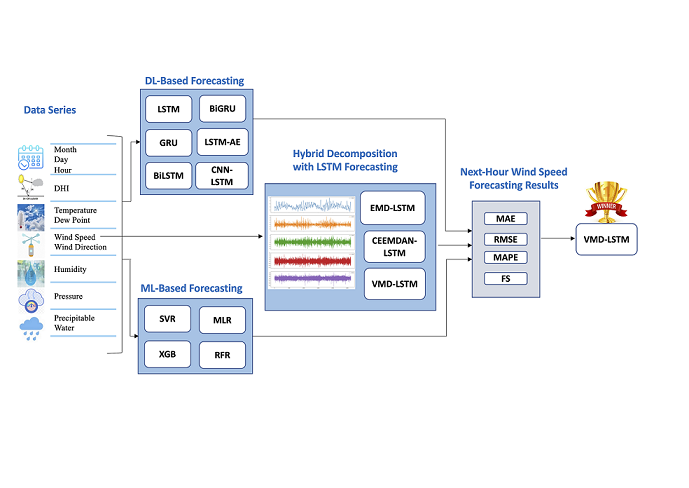
In this work, we propose a novel model that combines the variational mode decomposition (VMD) method and long short-term memory (LSTM) model, developed for next-hour wind speed prediction in a hot desert climate, such as the climate in Saudi Arabia. To test the superiority of the proposed model, we compared its performance with another twelve forecasting models: two hybrid models of decomposition methods and the LSTM model, six DL-based models, and four traditional ML-based models. Figure 1 provides a graphical abstract of the work, which shows the data inputs used, the forecasting models developed for comparison, and the evaluation metrics.
We summarize the contributions of this paper as follows.
  • We propose a novel hybrid model of the VMD method and LSTM model for next-hour wind speed prediction in a hot desert climate, such as the climate in Saudi Arabia. This is the first work, to our knowledge, proposing a hybrid model for this combination of task and weather.
  • We provide a performance comparison of the proposed model and two hybrid models of data decomposition techniques and the LSTM model, six DL-based models, and four ML-based models, using previous hours’ wind speed values only versus using weather variables besides wind speed values to show the effect of including weather variables on the forecasting performance.
  • Model performance comparisons are provided using data from four different locations in Saudi Arabia and two international locations, Caracas and Toronto. We present the results using visualization and several performance metrics, including mean absolute error (MAE), root mean square error (RMSE), mean absolute percentage error (MAPE), and forecast skills (FS).
We organize this paper into sections. Section 2 discusses the related works and highlights the research gap. Section 3 describes the methodology used in this paper, including data preprocessing steps, models’ development process, implementation details, and the evaluation metrics used to present the results. Next, Section 4 provides the results of wind speed (WS) forecasting based on the effect of using weather variables, the effect of seasonality, the effect of using decomposition methods, and the forecast skills of the models. Section 5 concludes the work.

2. Related Work

DL-based wind energy forecasting methods outperform other traditional methods, such as NWP, statistical, and conventional machine ML models, when making short-term predictions. We have performed an extensive literature review on DL-based wind energy forecasting methods in [11]. From our review and many other literature reviews of the renewable energy forecasting field [7,8,9,10], we noted a relationship between methods, terrain, and forecasting complexity. Method performances vary depending on the climate and terrain of the data source. The need for complex models differs based on the data. In some studies, ML methods, or shallow networks, provide satisfactory results with close performance to DL structures. In other studies, combining a decomposition method with a DL model has improved the forecasting performance.
There is a need for more studies that compare the prediction performance of ML methods using data gathered from different climates and terrains to reach a conclusion on the best method for certain data. For example, Manero et al. in [12] tested five DL models using wind data from around 126,000 locations in North America. They found that recurrent neural network (RNN) models perform better in desert areas, such as Nevada and Arizona. Also, they found that RNN and convolutional neural network (CNN) models provide better performance than the multilayer perceptron (MLP) neural network model for 1-hour ahead prediction, while the latter is better for 3 to 12-hour ahead prediction. Peng et al. proposed a hybrid model for wind speed forecasting that combines wavelet soft threshold denoising (WSTD) and gated recurrent unit (GRU) [13]. They tested their model using data from four locations in the United States with different climates. They found that the worst performance is associated with desert rock. Alhussein et al. [14] developed a model to predict wind speed and solar irradiance based on a multi-headed CNN using data from three locations in the United States with different climates, but they noted that different seasons and climates do not affect wind speed prediction results as solar radiation prediction.
In this work, we aim to enrich the literature by first proposing a novel model for wind speed prediction in a hot desert climate as in Saudi Arabia, and second by comparing the performance of several ML and DL models besides hybrid models for such climate using different datasets and features. The objective is to find the model and dataset features that achieve accurate predictions in a hot desert climate. We found several studies in the literature that used Saudi data, but to the best of our knowledge, none of them proposed hybrid models. Lawal et al. [15] compared the performance of linear, dense, CNN, and LSTM models with a hybrid model of CNN and bidirectional LSTM (BiLSTM) for next-hour wind speed prediction using data gathered from a location in Saudi Arabia. They found that the models’ performance at a height of 98 meters is better than 18 meters and the CNN-BiLSTM model performed the best. Faniband and Shaahid [16] compared the performance of three ML methods k-nearest neighbors (kNN), random forest, and support vector regression (SVR) to three statistical methods linear regression, Holt-Winter, and Auto Regressive Integrated Moving Average (ARIMA) for 1-hour ahead wind speed forecasting in Yanbu, Saudi Arabia. They found that ML methods provide better performance for 1-hour ahead prediction and SVR achieved the best performance. Zheng et al. [17] compared the performance of three ML models kernel ridge regression (RR), SVR, and artificial neural network for next-hour wind speed prediction using data from a city in Saudi Arabia. The comparison includes studying the effect of including weather variables besides wind speed and direction on prediction performance. Salman et al. [18] studied the effect that using three exogenous variables had on LSTM model performance for wind speed prediction using data from Dhahran, Saudi Arabia. They found that the best performance for 1 hour ahead is achieved with previous values of wind speed and temperature measured at 10 and 2 meters. Huang et al. [19] developed a spatio-temporal forecast model based on the echo state network (ESN) to predict wind speed in Saudi Arabia. They found the ESN model provides a more accurate prediction than the ARIMA method. Alharbi and Csala proposed a BiLSTM model in [20] and a GRU model in [21] to predict wind speed using data from Dumat Aljandal, Saudi Arabia. Both models provide similar performance. Tayeb Brahimi [22] used a feed forward neural network (FFNN) model with four hidden layers for hourly wind speed forecasting in four locations in Saudi Arabia. Faniband and Shaahid [23] used an FFNN model for hourly wind speed prediction. The dataset used to train and test their network was collected from Qaisumah, a village in the eastern province of Saudi Arabia. However, in both works [22,23], measurements of meteorological variables of the same prediction hour were used to train the models, which are unavailable in advance unless forecasted values are used.
Hybrid models that combine a decomposition method and a DL forecaster have proven their superiority in the wind energy forecasting field. Several works proposed hybrid models for wind speed prediction using data from locations with other climates than hot desert climates, such as China and the United States. For example, Liang et al. [24] developed a hybrid model of complete ensemble empirical mode decomposition with adaptive noise (CEEMDAN), permutation entropy (PE), GRU, radial basis function neural network (RBFNN), and an improved bat algorithm (IBA) for short-term wind speed forecasting for a wind farm in Zhangjiakou, China. The proposed model’s performance was compared to another eight ML models to validate its superiority. CEEMDAN in the proposed model was used to decompose wind speed data into several signals, then PE was calculated for each signal to combine closer ones into a smaller number of signals. Next, several GRUs were employed to extract the features from signals, which were fed into the RBFNN layer improved by IBA to produce the final prediction. In addition, Jiang et al. [25] developed a hybrid model of convolutional GRU, eXtreme gradient boosting (XGB) feature selection, and secondary decomposition method for multi-step wind speed forecasting for a wind farm in Shandong Province of China. Their secondary decomposition method starts with empirical mode decomposition (EMD) to decompose the original wind speed signal to several intrinsic mode functions (IMF), then VMD to further decompose the first IMF to several modes. For each subseries resulting from the decomposition stage, an XGB model was trained to extract the most important six features from the last 24-hour subseries, which were fed into a convolutional GRU that was optimized by genetic algorithm (GA) to provide forecasting results. This hybrid model outperformed another six ML models according to the comparison results. Lv and Wang [26] combined two decomposition methods: VMD and linear-nonlinear (LN) to decompose wind speed data and they used Multi-Objective Binary Back-tracking Search Algorithm (MOBBSA) to optimize the decomposition parameters. The final forecasting in their hybrid model results from averaging the outputs of multiple LSTM autoencoder sequence to sequence models. The proposed model in this work outperformed another four DL models in short-term wind speed forecasting for the Rocky Mountains, United States. Yildiz et al. [27] combined VMD and a residual-based CNN model for wind power forecasting using data from a wind farm in Turkey. They decomposed wind data by VMD, then reconstructed as 2D input images to be fed into a residual-based CNN model to produce forecasting. The performance of the proposed model was compared with five DL models to prove its improved accuracy. Wang et al. [28] developed a hybrid model for both wind power and wind speed forecasting, which combined VMD and Stacked Independently Recurrent Auto Encoder (SIRAE). Their model shows better performance than another four ML models. Hu et al. [29] proposed a hybrid model that combines VMD and ESN optimized by Differential Evolution algorithm (DE) for wind speed forecasting using data from a wind farm in Galicia, Spain. They validate the proposed model’s performance through comparison with six different models.
Table 1 summarizes the related work by specifying the forecasting objective, whether it is wind speed (WS) or wind power (WP), the forecasting method, features used as inputs, data source, whether it is ground-based measurements or simulation data, and the main results. If a work targets a prediction horizon other than the next-hour prediction, only the results of next-hour forecasting are included in the table.
Research Gap
As highlighted in this section, there is a need to develop new models designed for wind speed prediction in a hot desert climate. The literature in this field lacks comparative studies that show how ML and DL models perform under such climate conditions. To our knowledge, this is the first work proposing a hybrid model of a decomposition method and a DL model for such a climate. Also, it is important to quantify the improvement in the accuracy of DL models over ML with and without exogenous variables to show important data features. It is essential to highlight the performance gains of hybrid models over single models to justify the added complexity and help in making an informed decision on the tradeoff between accuracy and efficiency.

3. Methodology

We first describe data preprocessing steps in Section 3.1, including data collection, feature engineering, data normalization and portioning, and data decomposition methods. Then in Section 3.2, we describe the development process of seven DL models, which are LSTM, GRU, bidirectional LSTM (BiLSTM), bidirectional GRU (BiGRU), LSTM autoencoder (LSTM-AE), convolutional neural network LSTM (CNN-LSTM), and the hybrid model of decomposition methods and LSTM. We also describe four ML-based models, which are SVR, random forest regression (RFR), XGB, and multiple linear regression (MLR). In Section 3.3, we explain the implementation details of the models developed in this work. In Section 3.4, we clarify the performance evaluation metrics used for comparison.

3.1. Data Preprocessing

In this section, we describe four data preprocessing steps: data collection, feature engineering, data normalization and portioning, and data decomposition methods.

3.1.1. Data Collection

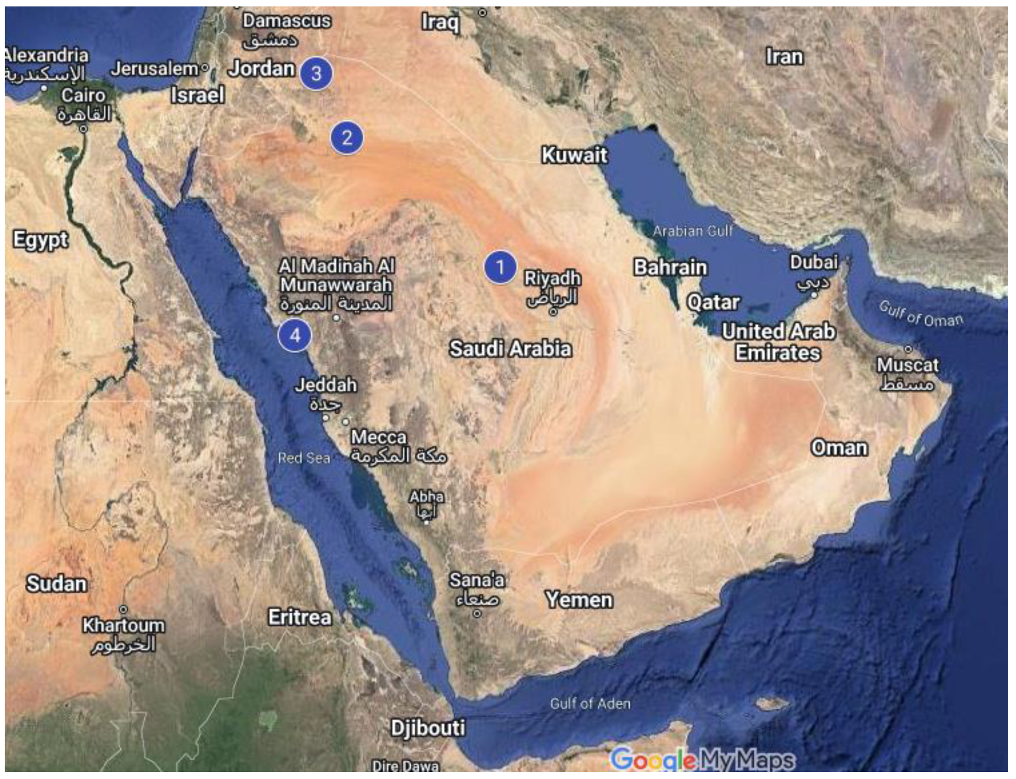
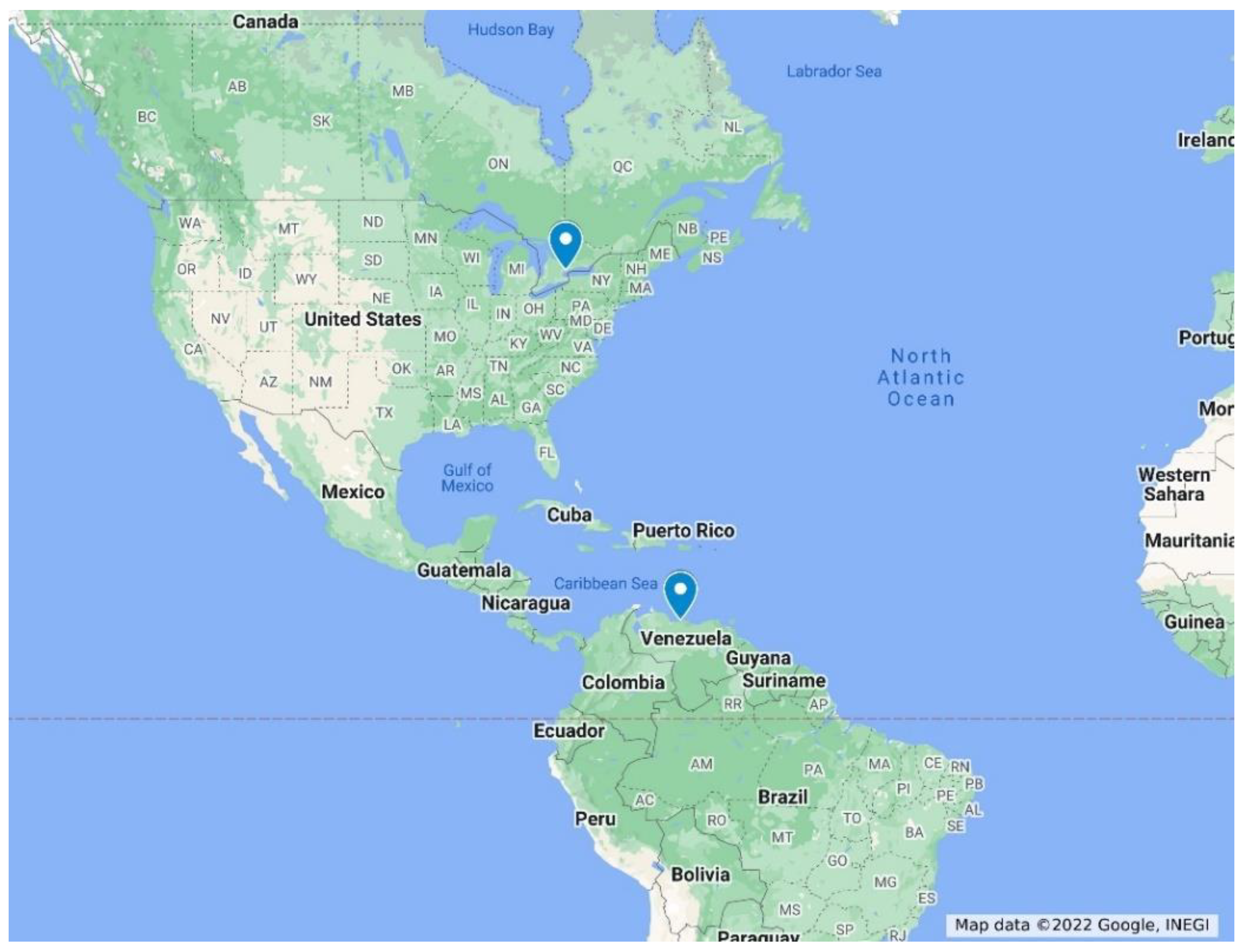
We used six datasets in this work from the National Solar Radiation Database (NSRDB) accessed through the National Renewable Energy Laboratory (NREL) website [30]. NREL notes the data is gathered by the METEOSAT IODC satellite and simulated by the Physical Solar Model (PSM) version 3 with a one-hour temporal resolution and 4 KM spatial resolution. The datasets cover the years 2017, 2018, and 2019. Four datasets were collected from locations in Saudi Arabia as shown in Figure 2, and two international datasets were collected from Caracas, Venezuela and Toronto, Canada, as shown in Figure 3. The climate classification of the Saudi locations is hot desert climate (BWh), whereas the climate classification of Toronto is humid continental (Dfb) and that of Caracas is tropical (A), according to the Köppen classification. Table 2 clarifies Saudi datasets locations information while Table 3 shows international datasets locations information.

3.1.2. Feature Engineering

Besides date and time information, all the datasets contain hourly values of 11 attributes:
  • Output: Wind Speed as a meter per second (m/s)
  • Wind Direction as degree (°)
  • Clear sky Global Horizontal Irradiance as watt per square meter (w/m2)
  • Clear sky Diffuse Horizontal Irradiance as w/m2
  • Clear sky Direct Normal Irradiance as w/m2
  • Precipitable Water (PW) as Millimeter
  • Temperature (T) as Celsius (°C)
  • Dew Point (DP) as Celsius (°C)
  • Pressure (P) as Millibar
  • Relative Humidity as a percentage (%)
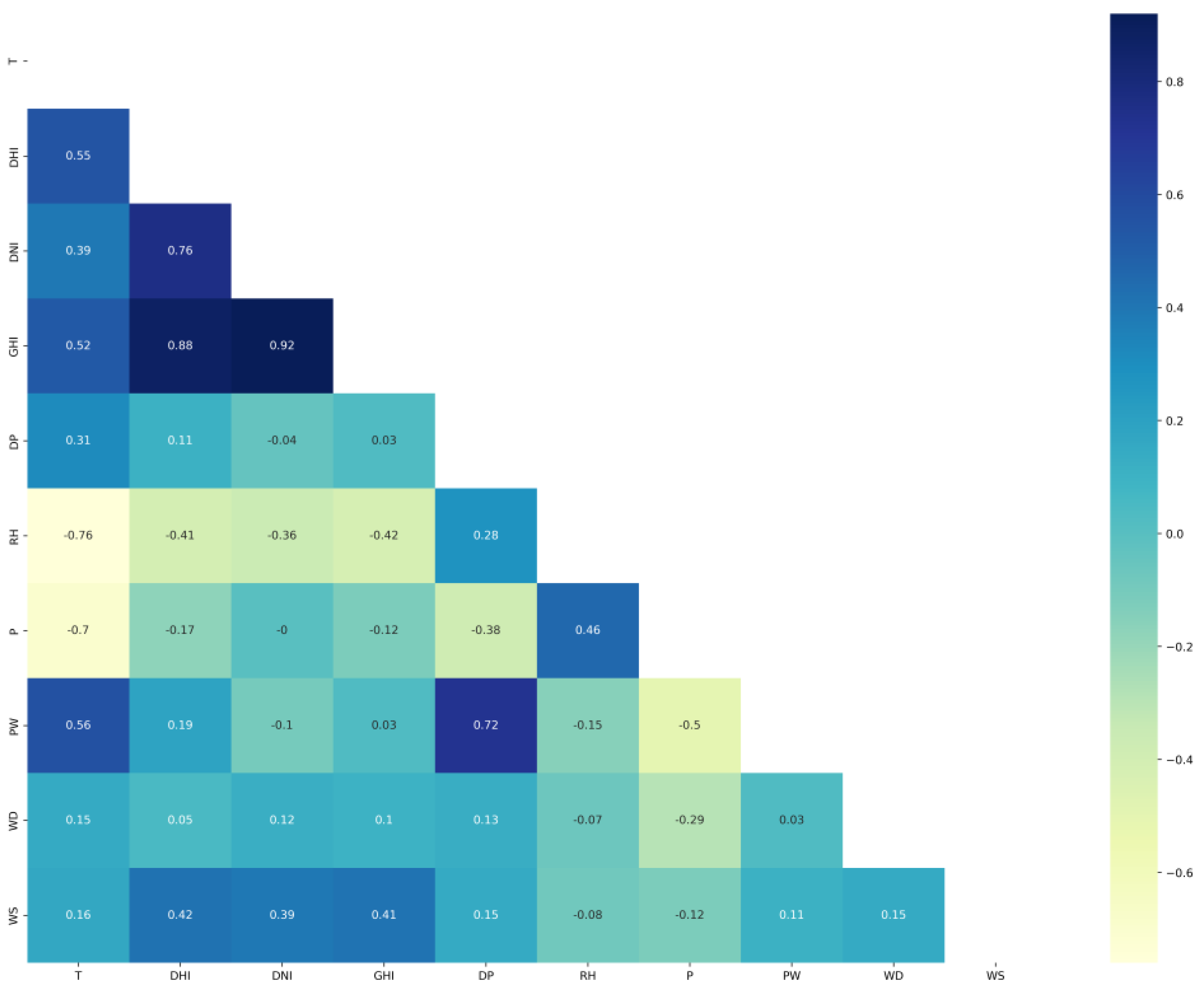
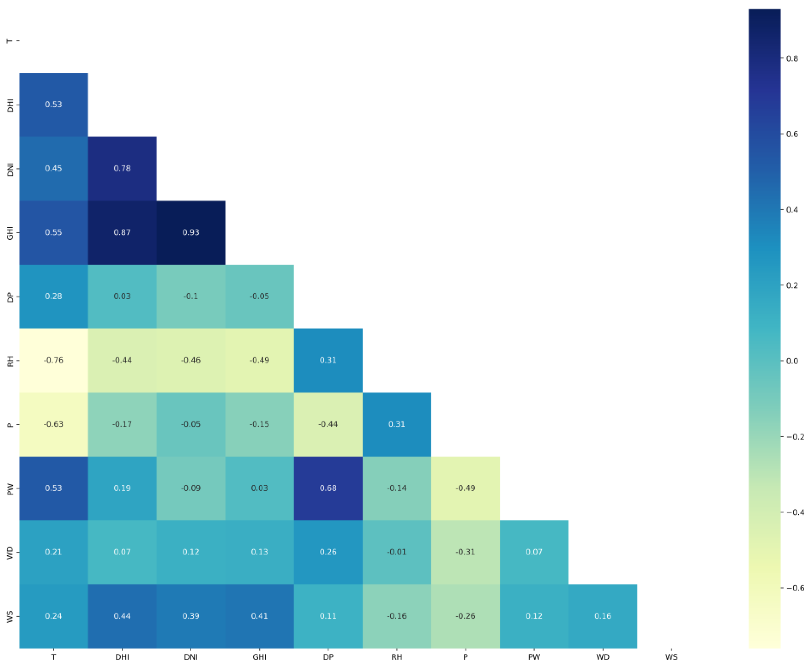
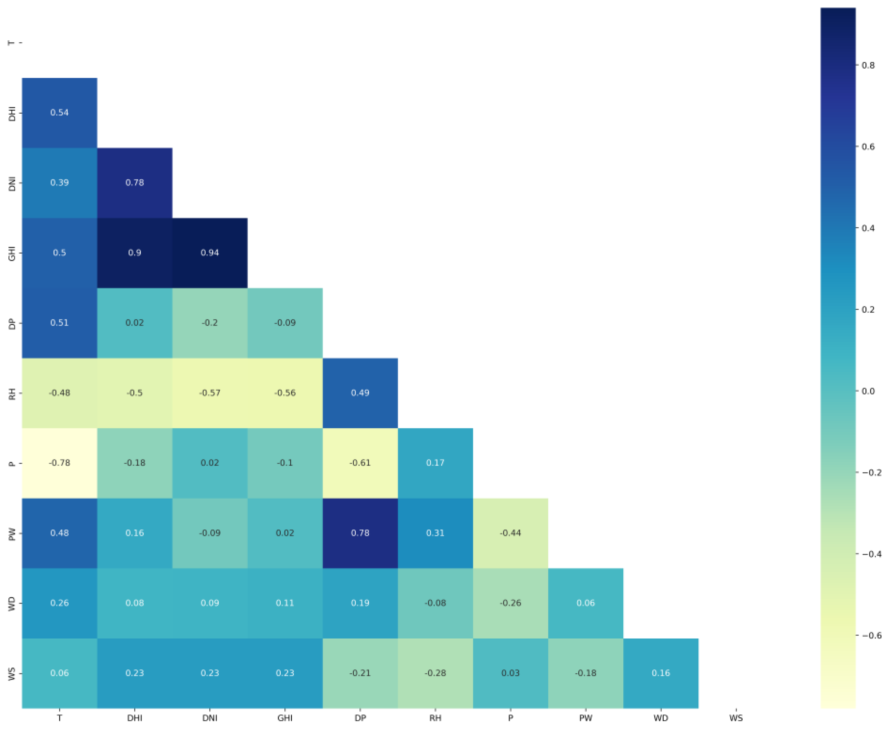
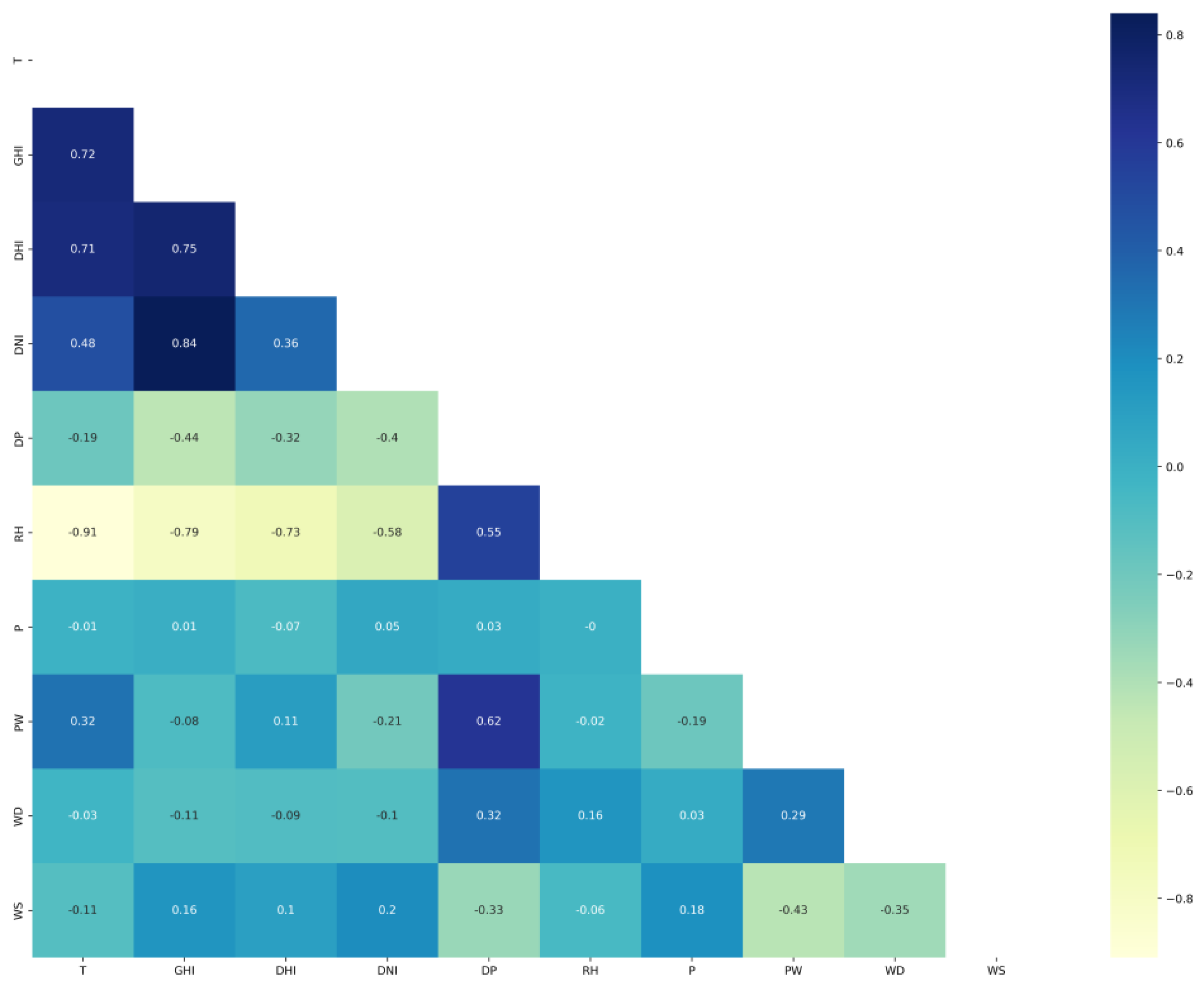
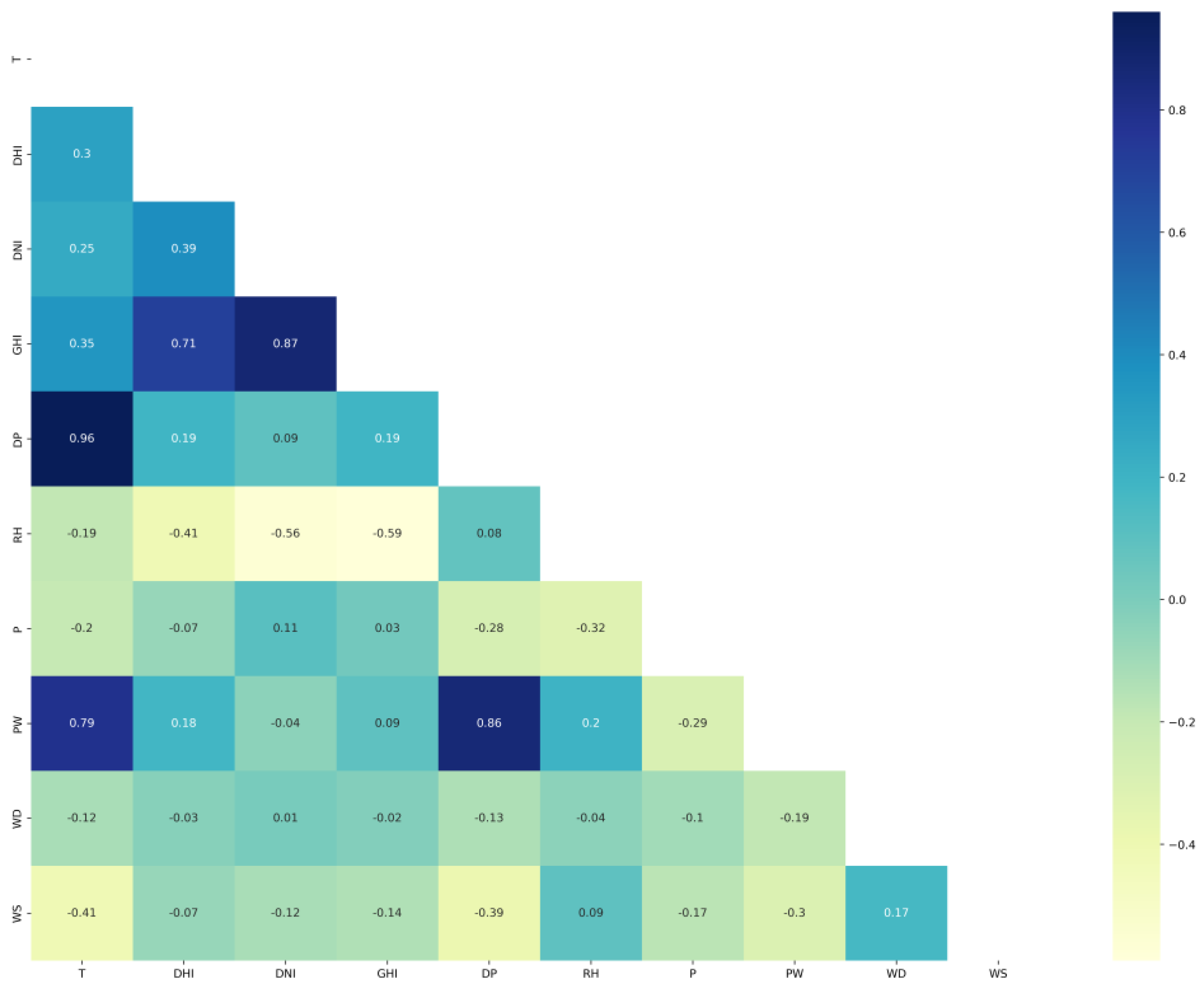
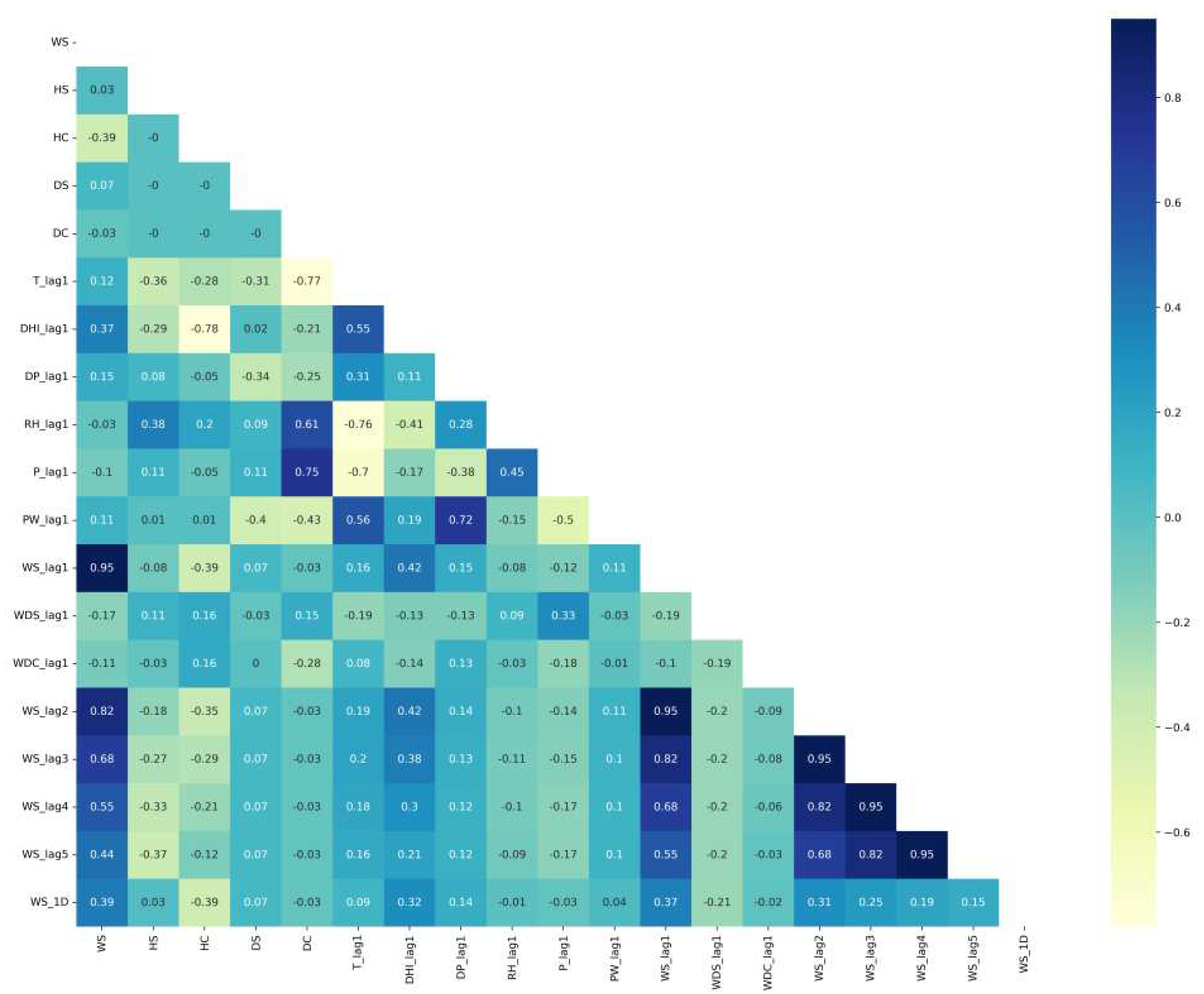
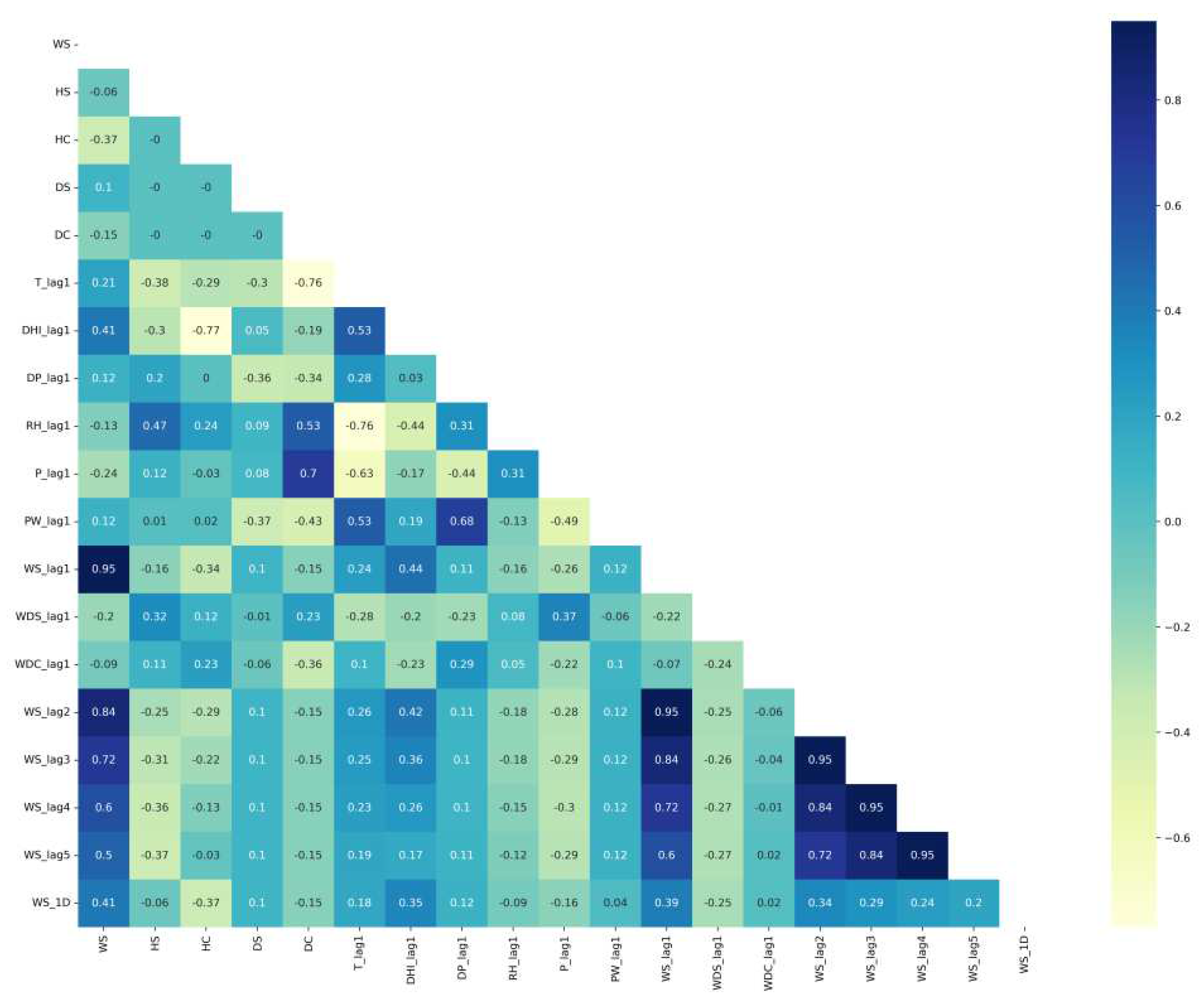
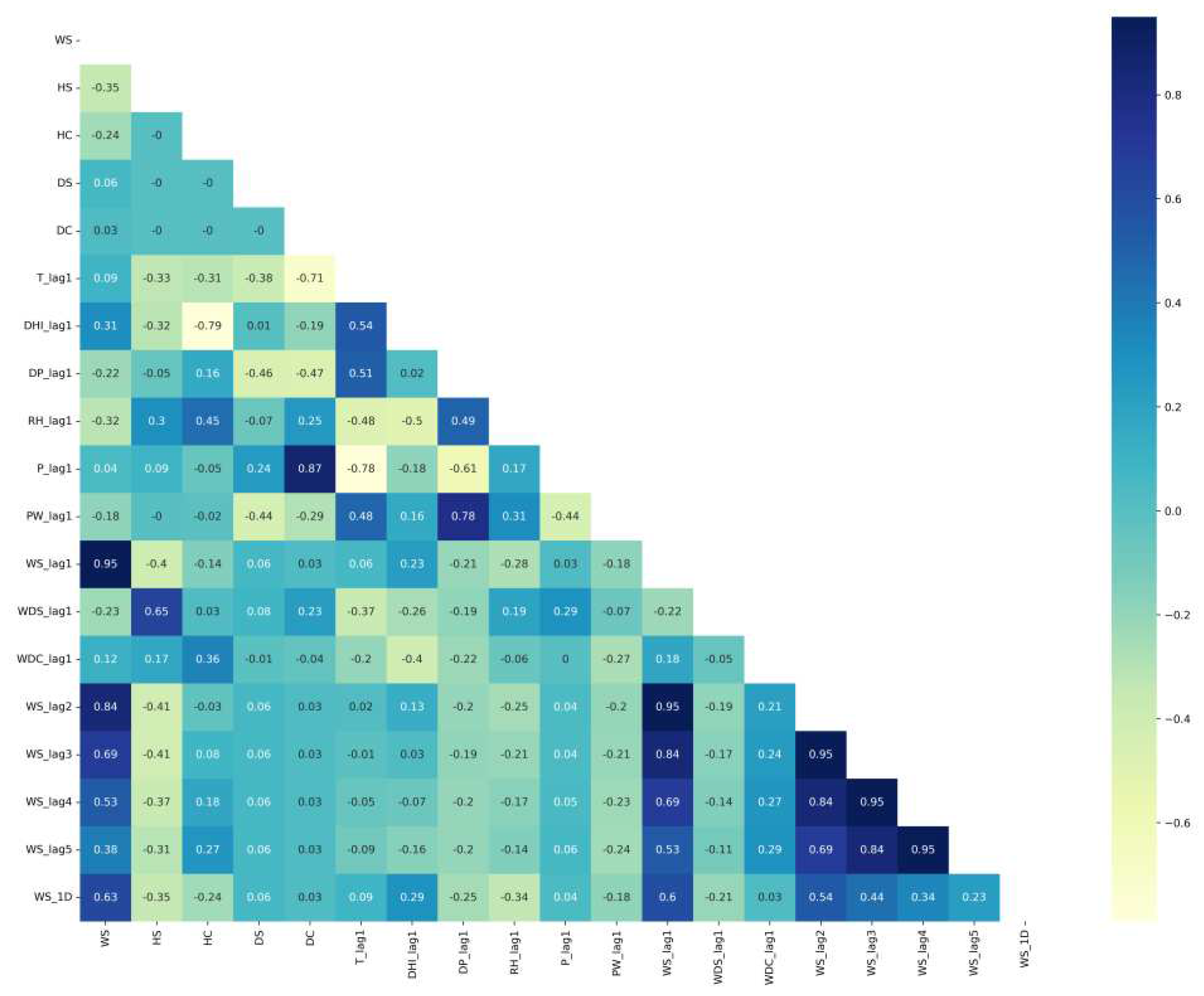
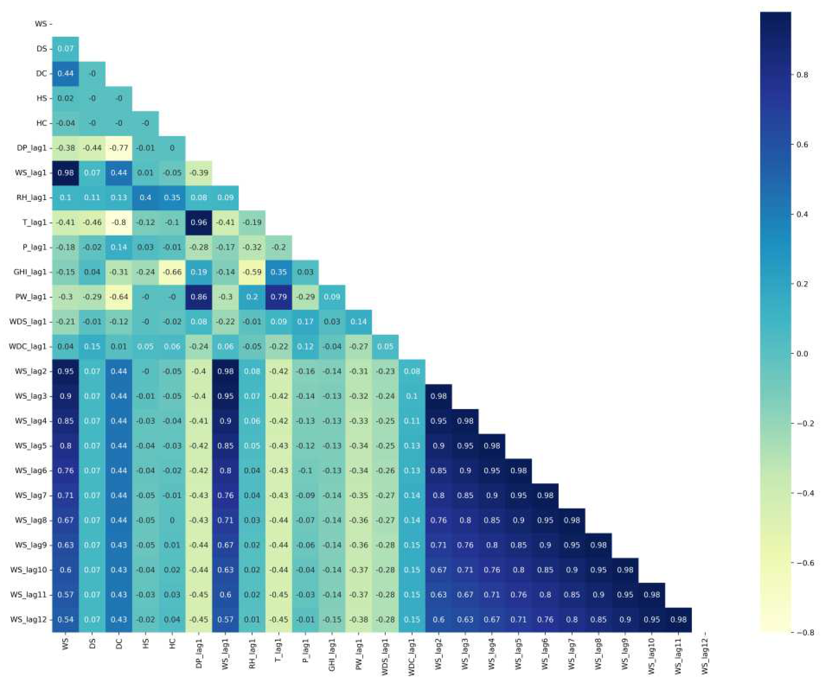
The correlation matrixes of Saudi locations are plotted in Figure 4 for Alghat, Figure 5 for Dumat Aljandal, Figure 6 for Waad Alshamal, and Figure 7 for Yanbu. From the correlation matrixes of these four locations, WS is positively correlated with WD, GHI, DHI, DNI, and T, whereas WS is negatively correlated with RH in all four locations. However, WS correlations with DP and PW are positive for Alghat, Dumat Aljandal, and Waad Alshamal, while they are negative for Yanbu. WS correlation with P is negative for Alghat, Dumat Aljandal, and Waad Alshamal, while it is positive for Yanbu. The strongest positive correlation of WS for all four datasets is with DHI and GHI, whereas the strongest negative correlation of WS is with P for Alghat, Dumat Aljandal, and Waad Alshamal, while it is with RH for Yanbu.
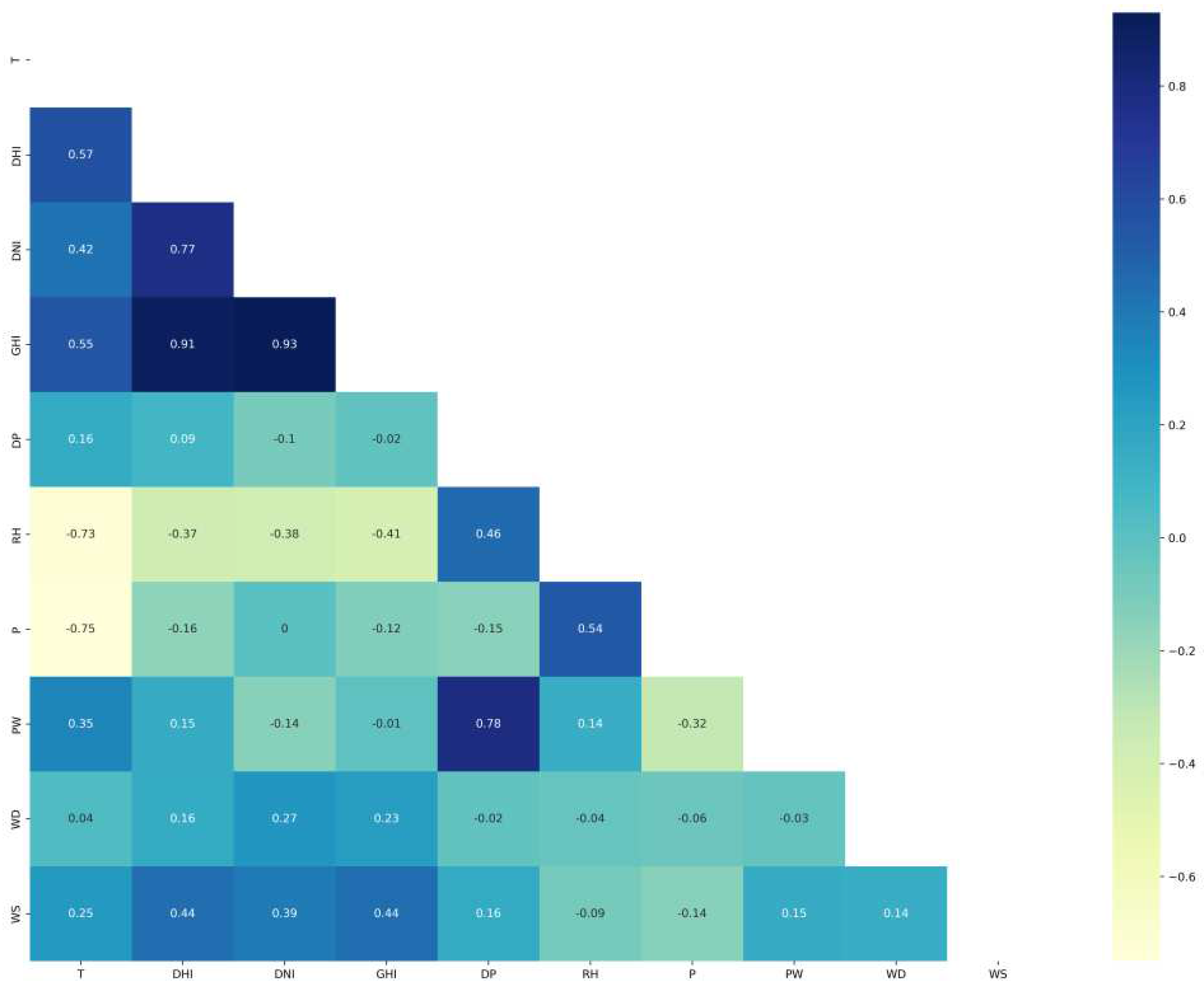
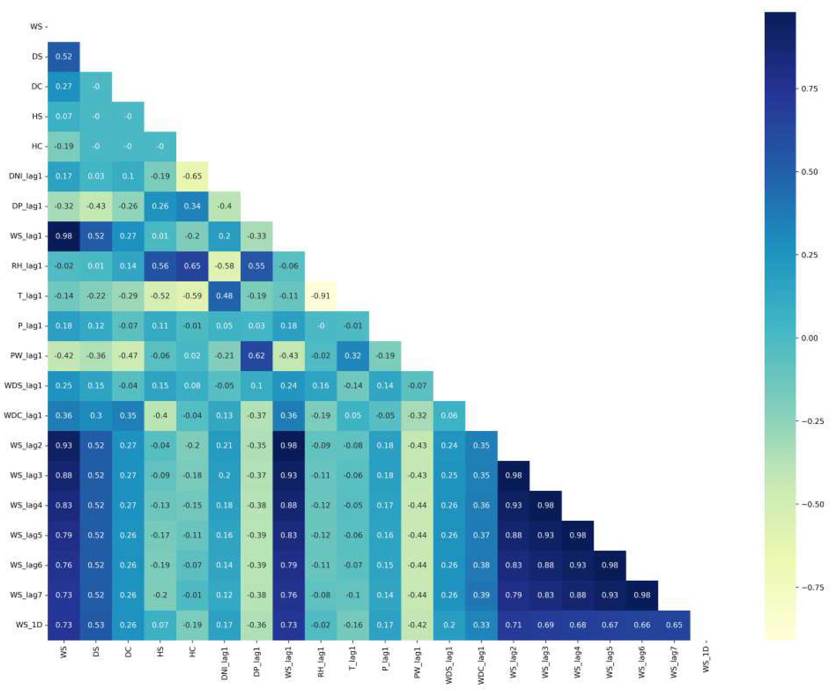
From the correlation matrix of Caracas in Figure 8, we note WS is positively correlated with GHI, DHI, DNI, and P, while WS is negatively correlated with T, DP, RH, PW, and WD. Also, positive correlations with WS are weak, whereas the strongest negative correlation with WS is with DP, PW, and WD. As appears in the Toronto correlation matrix in Figure 9, WS is negatively correlated with all variables except RH and WD and the strongest negative correlation of WS is with T and DP.
Since GHI, DNI, and DHI are all related to solar radiation information and are correlated, we nominated DHI to represent radiation in the Saudi datasets and eliminated DNI and GHI. DNI was chosen for the Caracas dataset, while GHI was chosen for the Toronto dataset because they have the highest correlations with WS. In addition, weather variables in the forecasting time (t) would not be available in reality, therefore, we used the last hour’s weather variables (at time t 1) as features to train the forecasting models, which include GHI_lag1, DP_lag1, RH_lag1, P_lag1, and PW_lag1. We did not use t 2 or t 3 weather variables because the correlations of time t 1 features with WS are insignificant (see Figure 11, Figure 12, Figure 13, Figure 14, Figure 15 and Figure 16), so there is no need to go further.
Temporal variables (month, day, hour) of the forecasting time (t) are also important inputs. We converted the day attribute to the Day of the Year. This eliminated the need to include the month number while also representing seasonality. For example, the first day of January will become Day 1 and the last day of December will become Day 365. Second, temporal variables have a cyclical nature. For example, Hour 23 is close to Hour 1 and Day 1 is close to Day 365. Treating temporal variables as regular numbers would make Hour 1 far from Hour 23, even though the difference is small. To avoid this problem that might affect the models’ learning, we eliminated the effect of the cyclical nature of temporal variables by encoding them into sine and cosine using the following equations [31]. The result is an additional four features: Hour Sine (HS), Hour Cosine (HC), Day Sine (DS), and Day Cosine (DC). We divided by 23 and 365 in equations 1 and 2 because 23 is the maximum hour in the datasets, whereas 365 is the maximum Day of the Year.
Wind direction has also a cyclical nature. For example, WD of value 10° is close to WD of value 360°. Therefore, we applied equations 1 and 2 and got an additional two features: WD Sine (WDS) and WD Cosine (WDC).
X ~ = sin 2 π   X max X    
X ~ = c os 2 π   X max X  
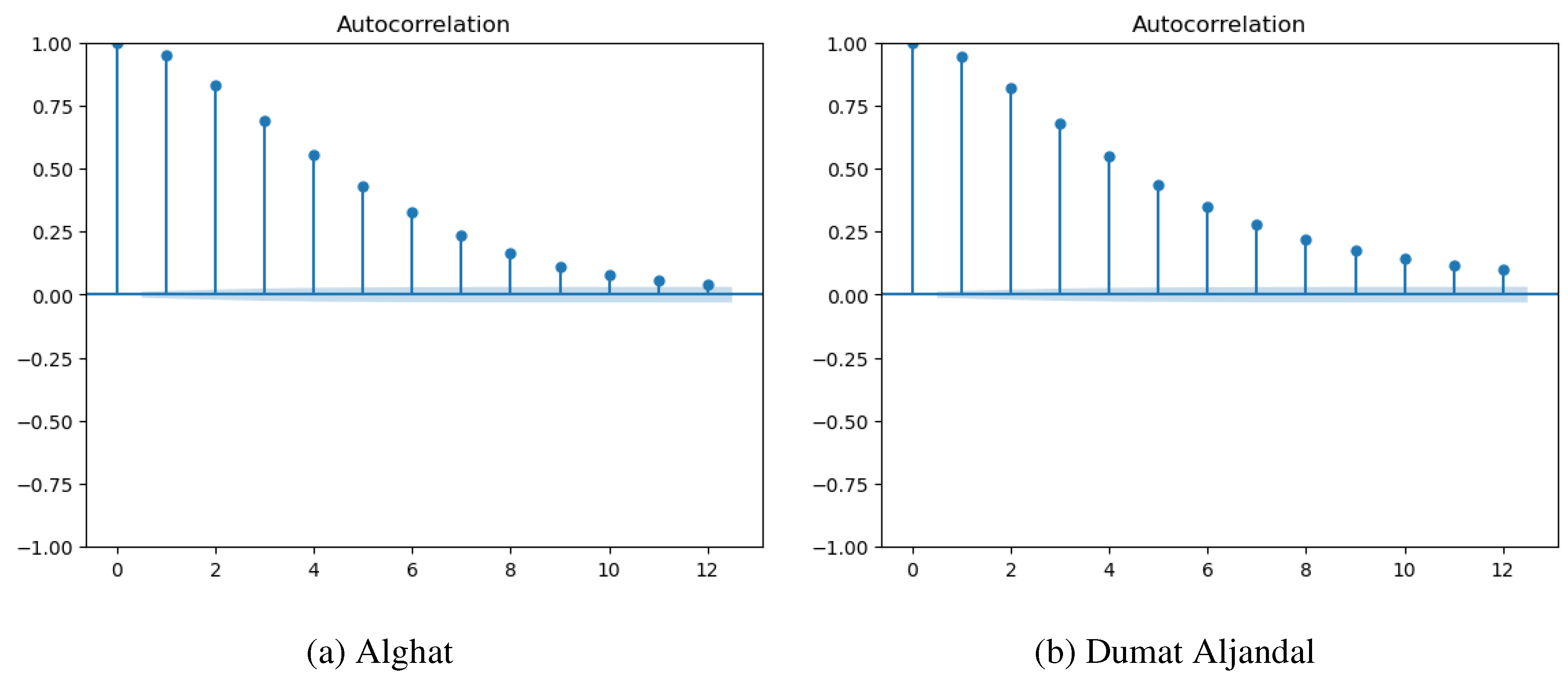
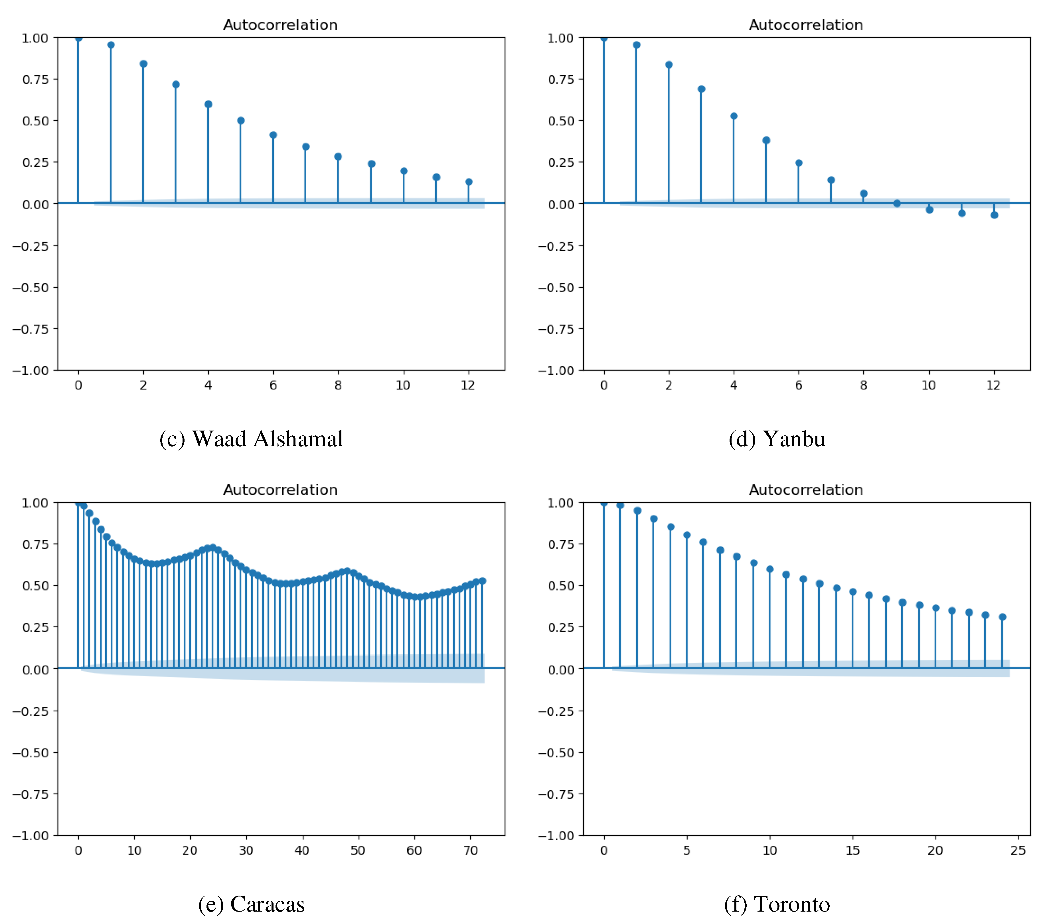
Lagged values of WS are essential inputs for making accurate forecasting. Therefore, we created WS lagged values with the shift method in the Pandas library. To guide the decision on lag, we used the autocorrelation function (ACF) for WS in each dataset, as presented in Figure 10. The ACF of Saudi datasets in Figure 10 (a), (b), (c), and (d) show a significant correlation of WS with its 5 past values. The correlation drops below 0.5 after lag 5. Therefore, we added WS values of the previous five hours to the feature set of Saudi datasets (WS_lag1, WS_lag2, WS_lag3, WS_lag4, WS_lag5). In addition, the last day same hour’s WS value might be important for forecasting, so we included it in the feature set (WS_1D) after checking its correlation with WS. The situation with Caracas and Toronto is different. In Caracas (see Figure 10 (e)), WS is significantly correlated with its 72 past values. Thus, we added WS_lag6, and WS_lag7 to the feature set. However, the correlation coefficient after WS_lag7 has the same value up to WS_1D, thus, we decided to only include WS_1D in the feature set to represent the trend and eliminate WS_lag8 to WS_lag23. In Toronto (see Figure 10 (f)), WS is significantly correlated with its 12 past values and correlation decreases afterward, so we added WS_lag8 to WS_lag12 to the feature set.
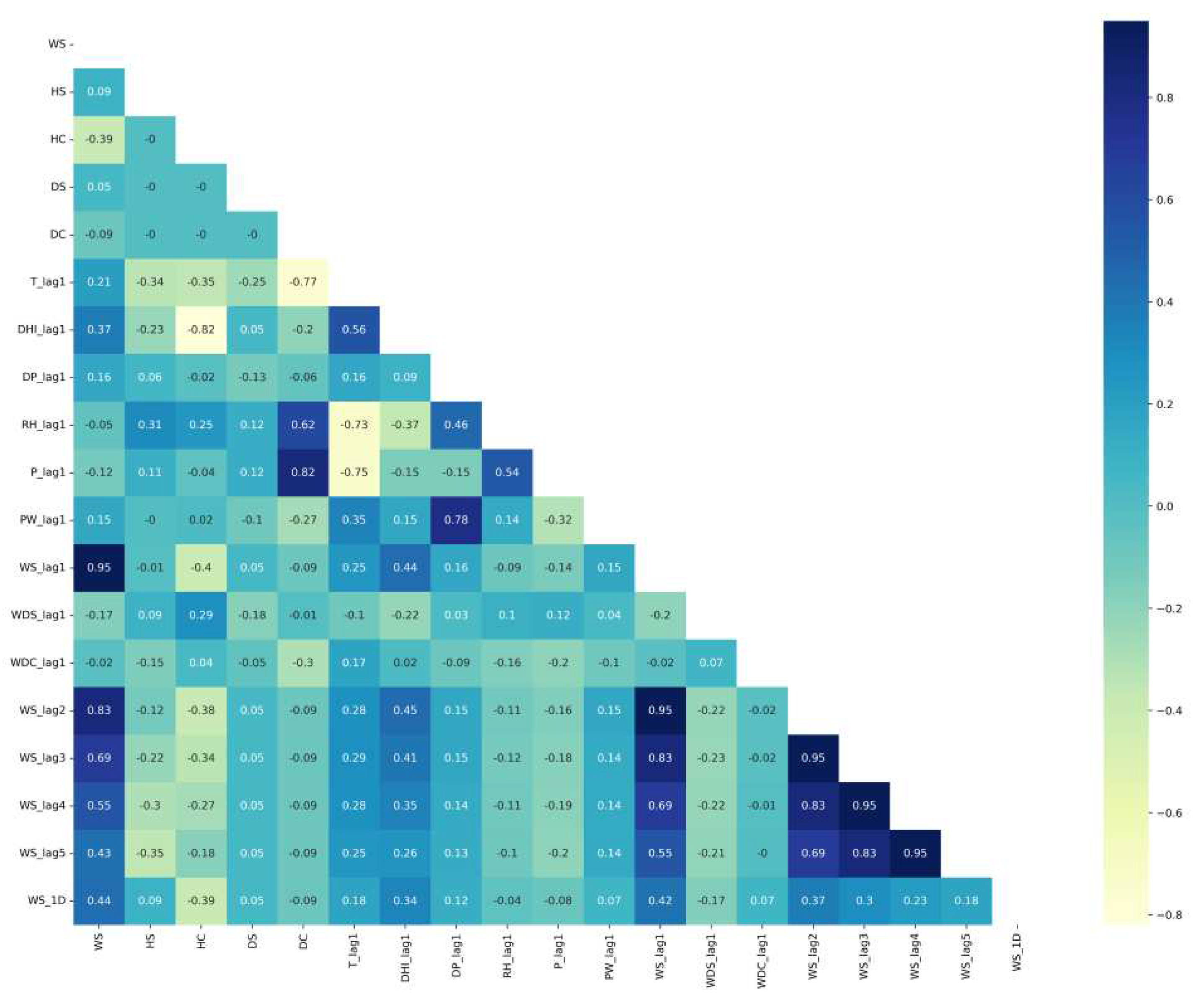
The final number of features in Saudi datasets after the feature engineering process is 18, as listed in Table 4. Figure 11 shows the correlation matrix of the Alghat dataset with these final features. If the threshold for significant correlation is +/−0.5, the correlations between WS and its past four hours’ values (WS_lag1 to WS_lag4) are significant. Figure 12 shows the correlation matrix of the Dumat Aljandal dataset with the final features, which has the same significant correlations as the Alghat dataset. Figure 13 displays the correlation matrix of the Waad Alshamal dataset in which the correlations between WS and its past five hours’ values (WS_lag1 to WS_lag5) are significant. Figure 14 shows the correlation matrix of the Yanbu dataset with these final features. WS has significant correlations with its past four hours’ values (WS_lag1 to WS_lag4) and WS value at the same hour on the last day, WS_1D.
The final number of features after the feature engineering process is 20 in the Caracas dataset and 24 for the Toronto dataset. Table 5 lists the common features among both datasets and shows the different features of each one. Figure 15 displays the correlation matrix of the Caracas dataset in which the correlation between WS and DS is significant, showing that the season has a strong effect on WS at Caracas. Also, the correlations between WS and its past hours’ values (WS_lag1 to WS_1D) are significant. Figure 16 displays the correlation matrix of Toronto in which the correlations between WS and its past 12 hours’ values (WS_lag1 to WS_lag12) are significant.

3.1.3. Data Normalization and Portioning

All features were normalized to the range of [0,1] using a min-max scaler, then denormalized to the normal range after the training process was complete and before calculating the evaluation metrics. We portioned data into 70% for training, 15% for validation, and 15% for testing. The total number of records for each dataset is 26255, out of which 18410 records are used for training, 3906 used for validation, and 3939 used for testing. Table 6 describes each dataset used in this work. It defines mean, standard deviation, variance (VAR), minimum (MIN), and maximum (MAX) values of WS in each data portion and in the dataset entirely.

3.1.4. Data Decomposition Methods

We have performed two tests to check the stationarity of wind speed data, which are the Dickey-Fuller (AD) test and the Kwiatkowski, Phillips, Schmidt, and Shin (KPSS) test. Even though both tests showed data is stationary, we tried data decomposition methods and checked their effect on forecasting. Section 4 shows the improvement in prediction results after using three methods: EMD, CEEMDAN, and VMD. In this section, we describe these three methods.

3.1.4.1. EMD

The EMD method decomposes a time series into a set of IMFs with different frequency bands and a residue based on the local properties of the time series. EMD effectiveness is proven in a broad range of applications for analyzing nonlinear and nonstationary processes. However, there are still some limitations to applying EMD. One of the major limitations is the mode mixing problem. Mode mixing means that a signal of different scales exists in one IMF or a signal of a similar scale exists in different IMFs [32,33].
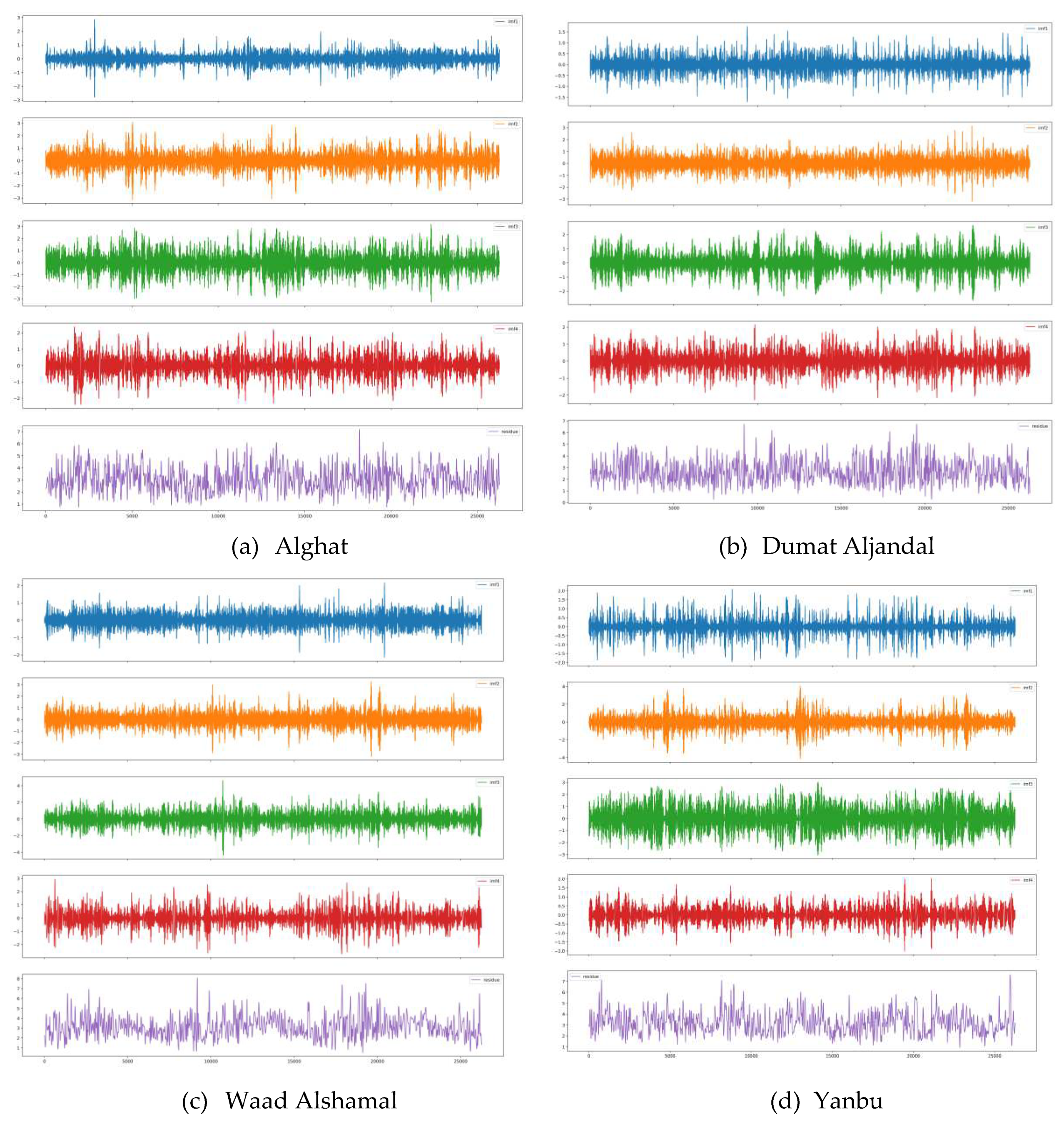
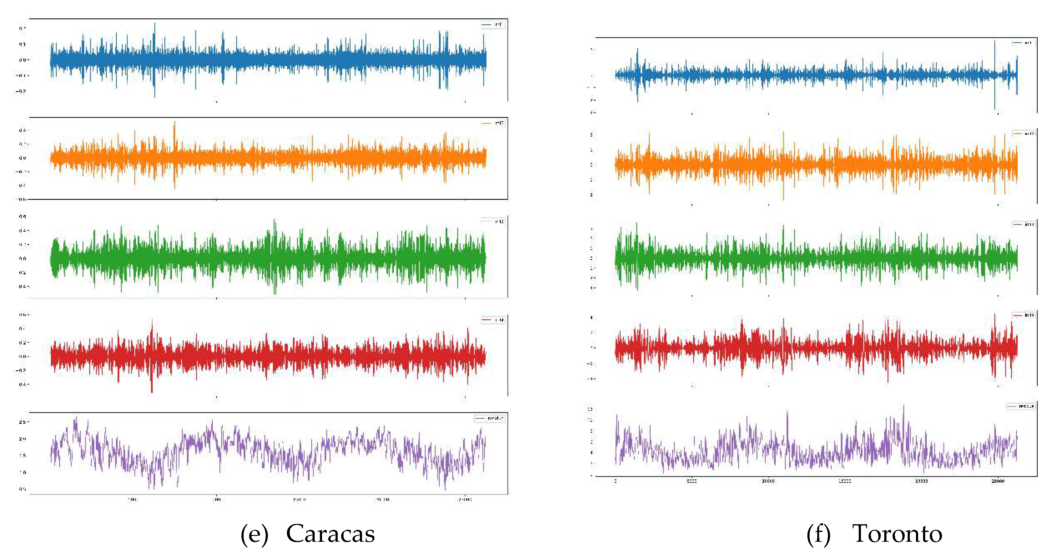
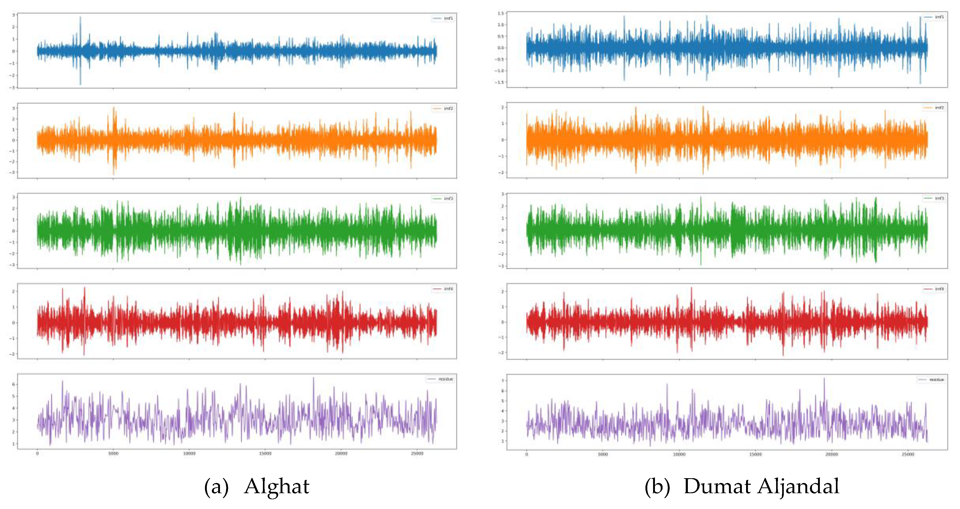
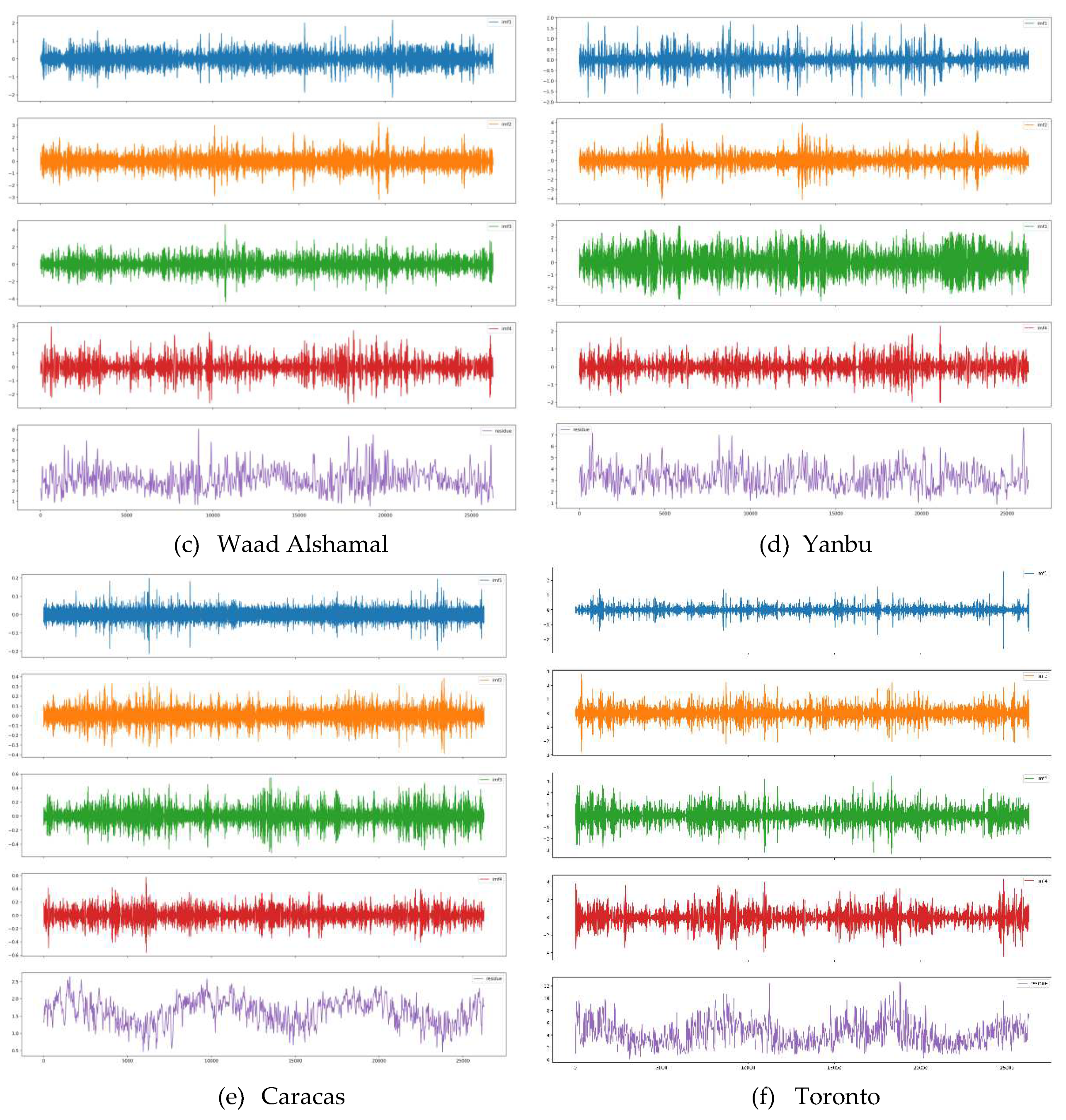
EMD results of WS decomposition for all datasets are illustrated in Figure 17. Without limiting the number of IMFs, EMD decomposes WS into eleven IMFs and a residue. However, we set the maximum number of IMFs to 4 after the trial-and-error process because we have not seen an improvement in forecasting with a bigger number.

3.1.4.2. CEEMDAN

To address the mode mixing problems in EMD, various improved EMD methods were proposed and CEEMDAN is one of the latest versions. CEEMDAN can solve the mode mixing problem without adding extra noise to the reconstructed signal [32,33].
CEEMDAN results of WS decomposition for all datasets are illustrated in Figure 18. Without limiting the number of IMFs, CEEMDAN decomposes WS into eleven or twelve IMFs and a residue. However, we set the maximum number of IMF to 4 after the trial-and-error process because we have not seen an improvement in forecasting with a bigger number.

3.1.4.3. VMD

VMD is an effective decomposition algorithm that decomposes a time series into several modes, which have specific sparsity properties while producing the original time series [32,33]. VMD-based models show better noise robustness and more precise component separation.
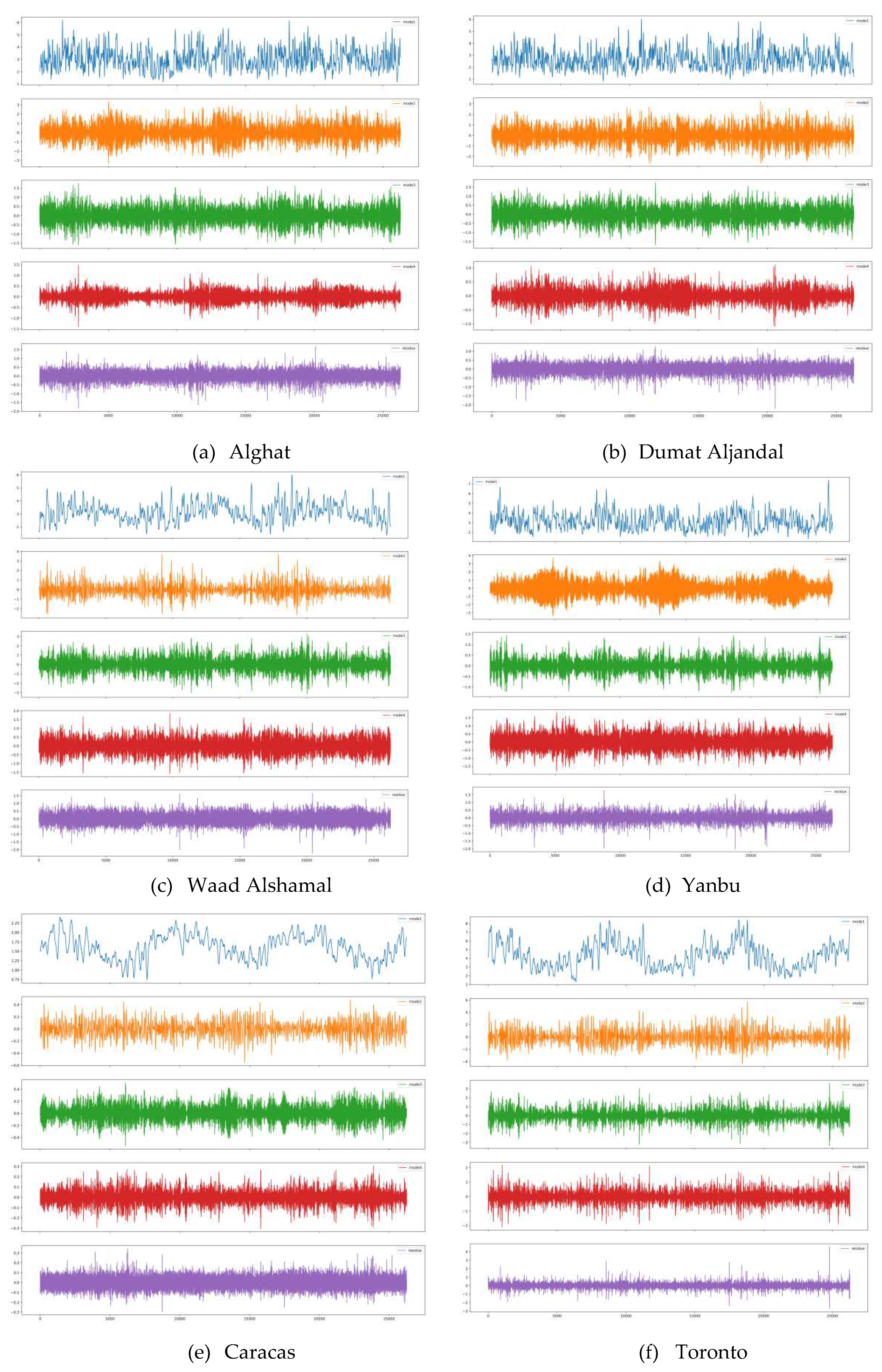
VMD results of WS decomposition for all datasets are illustrated in Figure 19. We set the number of modes to 4 based on the trial-and-error process because we have not seen an improvement in forecasting with a bigger number.

3.2. Models’ Development

In Section 3.2.1, we describe seven DL-based models: LSTM, GRU, BiLSTM, BiGRU, LSTM-AE, CNN-LSTM, and the hybrid model of a decomposition method and LSTM. We describe four ML-based models in Section 3.2.2: SVR, RFR, XGB, and MLR.

3.2.1. DL-Based Models

Seven DL-based models are described here, which are used for next-hour WS forecasting. These models are LSTM, GRU, BiLSTM, BiGRU, LSTM-AE, CNN-LSTM, and the hybrid model of a decomposition method and LSTM.

3.2.1.1. LSTM

LSTM is a special type of RNN that can learn long-term dependencies. It performs better than traditional RNN in diverse tasks. Besides the hidden state, LSTMs contain the cell state that conveys important inputs from previous steps to later steps. Meanwhile, new inputs are added to or deleted from the cell state through input and forget gates. The output gate determines if the current memory cell will be output. More details on LSTM are in [34,35].
An LSTM model for the next-hour WS forecasting is implemented in this work, as clarified in Figure 20, which comprises two LSTM layers for feature extraction and two dense layers to make WS prediction. The activation function of the LSTM model is ReLU. Further implementation details are given in Section 3.3.

3.2.1.2. GRU

GRU is like LSTM because it captures long-term dependencies but does not contain the cell state. The update gate in GRU determines the amount of past information that needs to be kept because the reset gate determines how much to forget. GRUs are often faster and need less computation time and memory than LSTMs [36].
A GRU model for the next-hour WS forecasting is implemented in this work, as clarified in Figure 21, which comprises two GRU layers for feature extraction and two dense layers to make a WS prediction. More implementation details are given in Section 3.3.

3.2.1.3. BiLSTM

BiLSTM is an adjusted version of LSTM that contains two layers: one to process inputs in a forward direction, and another to process inputs in a backward direction. This structure allows learning from past and future information. More details on BiLSTMs are in [20,34].
BiLSTM model for the next-hour WS forecasting is implemented in this work, as clarified in Figure 22. It comprises one BiLSTM layer, and one LSTM layer, followed by two dense layers to make WS prediction. More implementation details are given in Section 3.3.

3.2.1.4. BiGRU

Similar to BiLSTM, BiGRU comprises two GRUs, which process the input sequence from two directions, then merge their representations [37].
A BiGRU model for the next-hour WS forecasting is implemented in this work, as clarified in Figure 23. It comprises one BiGRU layer, and one GRU layer, followed by two dense layers to make WS prediction. More implementation details are given in Section 3.3.

3.2.1.5. LSTM-AE

Autoencoder is a neural network that comprises two parts: the encoder and the decoder. The encoder compresses inputs into a feature vector called latent space, and the decoder decompresses it into output. This data reconstruction process helps the model extract the most important features. The LSTM-AE model is an autoencoder in which both the encoder and decoder comprise LSTM layers to learn temporal dependencies in sequence data. Work in [38] and [39] contains more on LSTM-AE.
An LSTM-AE model for the next-hour WS forecasting is implemented in this work, as clarified in Figure 24. Both the encoder and decoder have two LSTM layers, followed by two dense layers to make WS prediction. More implementation details are given in Section 3.3.

3.2.1.6. CNN-LSTM

In CNN and LSTM structure, convolutional and pooling layers are followed by LSTM layers, then one or more dense layers to generate the output [40].
A CNN-LSTM model for the next-hour WS forecasting is implemented in this work as clarified in Figure 25, which comprises two 1D convolutional layers with kernel size equals 2, a max-pooling layer, a flatten layer, a repeat vector layer, an LSTM layer, a dropout layer, and two dense layers. Section provides more implementation details.

3.2.1.7. Hybrid Model of Decomposition Methods and LSTM

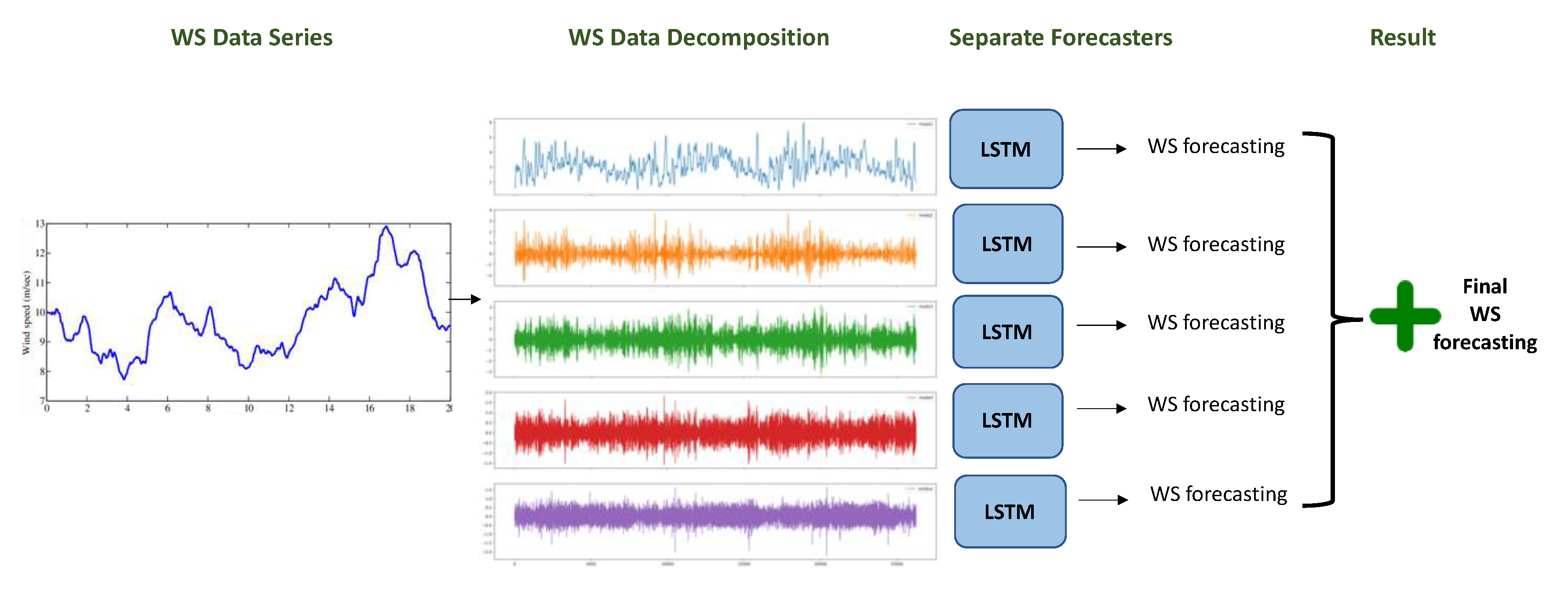
The LSTM model, combined with the decomposition methods (EMD, CEEMDAN, VMD), is the same model illustrated in Section 3.2.1.1. However, the activation function is Tanh instead of ReLU, as appears in Figure 26 because the decomposition process produces negative values for which Tanh is more suitable (refer to Figure 17, Figure 18, and Figure 19 to see the range of decomposition results). To understand how the hybrid model works, Figure 27 clarifies the forecasting process, which starts with applying a decomposition method on WS original data series, then uses a separate LSTM model for each subseries. The results of these separate LSTM models are totaled to provide the final WS forecasting.

3.2.2. ML-Based Models

In this section, we describe four ML-based models used in this work for performance comparison, which are SVR, RFR, XGB, and MLR.

3.2.1.1. SVR

SVR is a supervised ML algorithm for regression problems, which recognizes non-linearity in the data. It predicts values instead of predicting classes as a support vector machine that is used for classification problems. In SVR, the best-fit line is the hyperplane that has the maximum number of points [41].
In this work, the SVR was built using Scikit-learn library with radial basis function kernel, with the parameter settings: C = 100; epsilon = 0.001. It was trained and tested using the same training and testing sets of the datasets described in Table 6.

3.2.1.2. RFR

Random forest is a non-parametric, supervised, and ensemble-based learning method used for both classification and regression tasks. Its final output is the average of multiple decision trees’ outputs. Therefore, it produces a more accurate prediction than a single decision tree [42].
In this work, the RFR, which was built using Scikit-learn library, has 600 estimators with a maximum depth equal to 50. It was trained and tested using the same training and testing sets of the datasets described in Table 6.

3.2.1.3. XGB

XGB is a scalable, distributed gradient-boosted decision tree. It is an ensemble learning algorithm, like a random forest for classification and regression. Gradient boosting improves a single weak model by combining it with several other weak models to generate a strong ensemble model. XGB is an accurate and efficient implementation of gradient boosting that uses computing power for building trees in parallel [25].
In this work, the XGB, which was built using XGBoost library, has 500 estimators with a learning rate equal to 0.1. It was trained and tested using the same training and testing sets of the datasets described in Table 6.

3.2.1.4. MLR

MLR is a conventional statistical method to define the relationship between multiple independent variables and one dependent variable. This relationship is represented by the following equation:
y =     β 0 + β 1   X 1 + β 2   X 2 + β 3   X 3 + ε
where y is the dependent variable, X is the independent variable, β is the regression coefficient, and ε is the residual error [43].
In this work, the MLR was built using Scikit-learn library and the same training and testing sets of the datasets described in Table 6.

3.3. Implementation

In this work, the Keras Library, a DL API written in Python and running on top of the TensorFlow platform, was used to create DL models, where Python3 was employed as the programming language. The PyEMD library was used for EMD and CEEMDAN, whereas the vmdpy library was used for VMD. The experiments were performed on a laptop with Intel Core i7-11800 H CPU, NVIDIA GeForce RTX 3070 GPU, and 16 GB memory. However, all DL models were developed using the GPU. Table 7 specifies the hyperparameters used in developing DL models, besides the optimization methods. The structures of all DL model including the type and number of layers and their neurons, are illustrated in Section 3.2.1.

3.4. Evaluation Metrics

In this work, four performance evaluation metrics are used to evaluate the forecasting models.
Mean absolute error is the mean of the absolute values of the individual forecast errors on overall examples (N) in the test set. Each forecasting error is the difference between the actual value (actual WS) and the forecast value (forecast WS). A lower value of MAE is better. It is calculated as follows [44].
M A E = 1 N i = 1 N a c t u a l   W S i f o r e c a s t   W S i
Root Mean Square Error is the standard deviation of the residuals or the forecast errors. It measures residual spread and how the data is concentrated around the line of regression. A lower value of RMSE is better. RMSE is calculated as follows [44].
R M S E = 1 N i = 1 N ( a c t u a l   W S i f o r e c a s t   W S i ) 2
Mean absolute percentage error is a measure of forecasting accuracy. This percentage shows the average difference between the forecasted value and the actual value. Smaller MAPE provides better forecasts. MAPE is calculated as follows [45].
M A P E = 1 N i = 1 N a c t u a l   W S i f o r e c a s t   W S i a c t u a l   W S i × 100 %
Forecast skills are used to compare a proposed forecasting model performance metric with a reference model performance metric. An often-used reference model in the literature is the persistence method. The evaluation metric could be RMSE, MAE, or others. FS is calculated as follows [46].
F S = 1 M e t r i c p r o p o s e d M e t r i c   p e r s i s t e n c e   * 100 %

4. Results and Discussion

In this section, we present and discuss the results of the models’ forecasting performance from four aspects: the effect of using weather variables besides lagged wind speed features on forecasting accuracy (Section 4.1); the effect of seasonality on forecasting accuracy (Section 4.2); the effect of using three decomposition methods with the LSTM model for forecasting accuracy (Section 4.3); and the percentage of the forecasting improvement of all models over the persistence method, known as the Forecast Skill (Section 4.4).

4.1. Effect of Using Last Hour’s Weather Variables on Forecasting

To study this effect on Saudi datasets, ten forecasting models were trained and tested twice with the same records. First, training was conducted using 18 features as shown in Table 8, which include temporal features, the last hour’s weather variables, and WS values of the previous 5 hours besides the WS value of the same hour last day. In the second trial, only WS values of the previous 5 hours were used, as highlighted in Table 8. For the Caracas dataset, 20 features were used in the first trial (with WS_lag6, and WS_lag7 added to Table 8 features) and 7 features in the second trial (WS_lag1 to WS_lag7). For the Toronto dataset, 24 features were used in the first trial (with WS_lag8 to WS_lag12 added to Table 8 features and WS_1D removed). In the second trial for the Toronto dataset, only 12 features were used (WS_lag1 to WS_lag12).
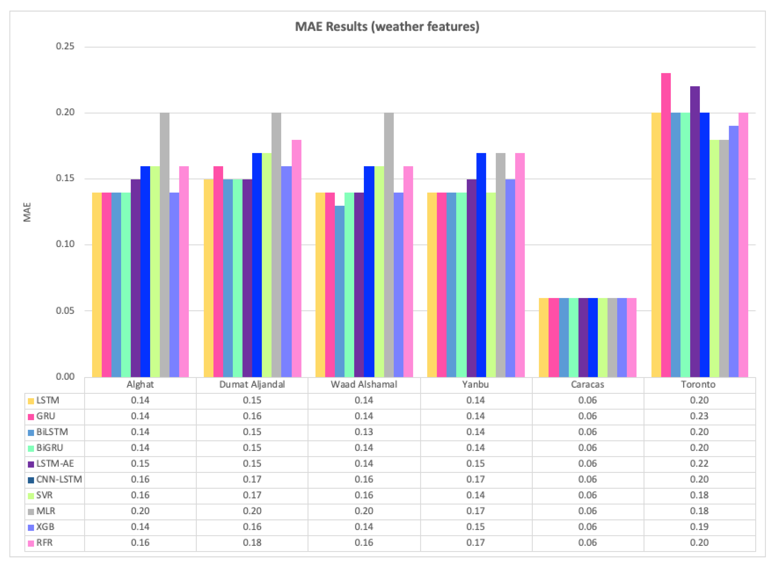
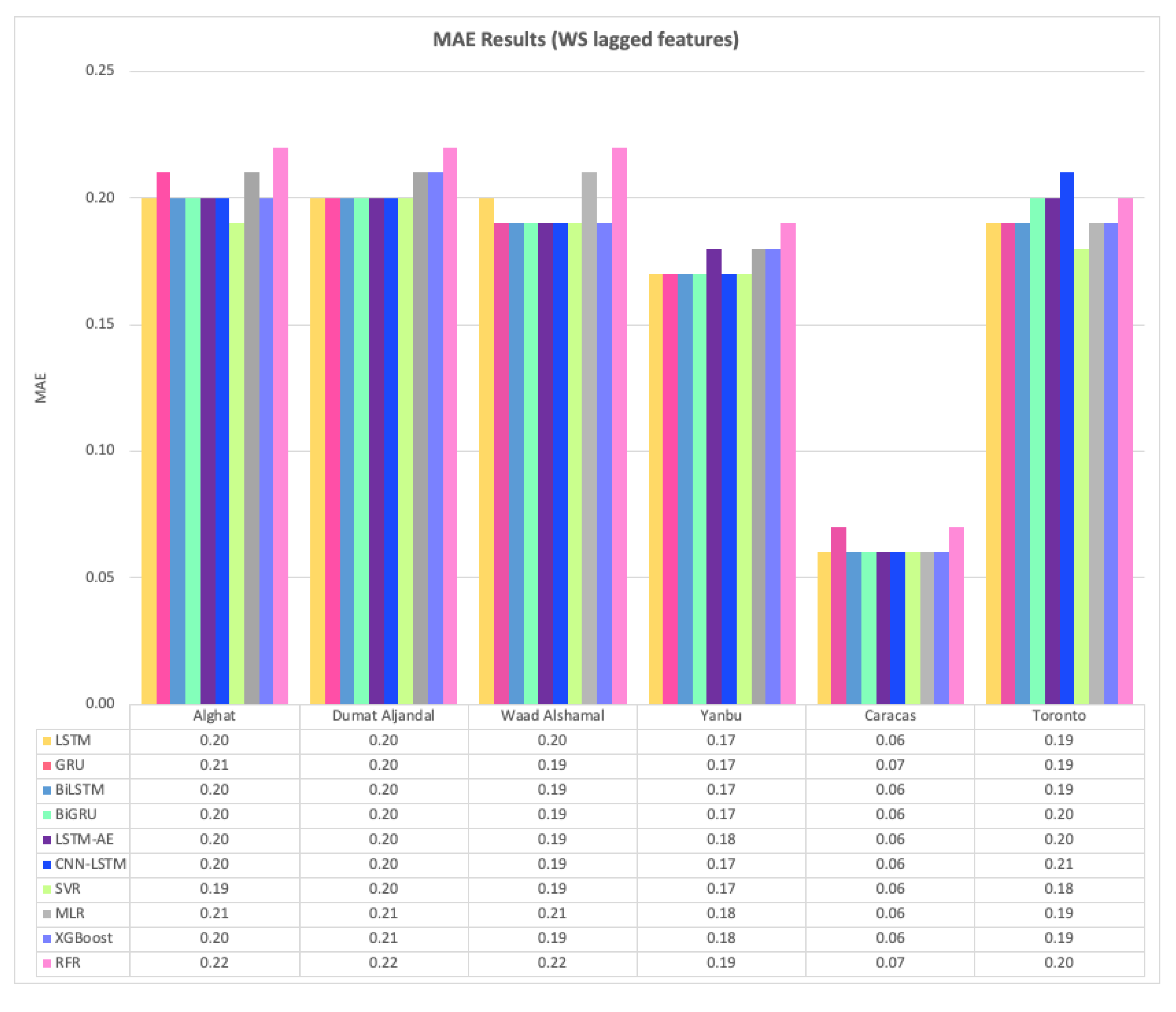
Figure 28 shows the average MAE results of 20 runs of the six DL-based forecasting models and four ML-based models when weather features were used besides WS lagged features, whereas Figure 29 shows the same when only WS lagged features were used.
For Alghat dataset, we noted that using weather features has improved the MAE results for all six DL-based forecasting models by 33% at most as with the GRU model and 20% at least as with the CNN-LSTM model. Using weather features in ML-based models improved the MAE results for all four models by 30% at most as with the XGB model and 5% at least as with MLR model. The best MAE value is 0.14 achieved by LSTM, GRU, BiLSTM, BiGRU, and XGB models, while the worst MAE value is 0.20 and associated with the MLR model.
For Dumat Aljandal dataset, using weather features has improved MAE results for all six DL-based forecasting models by 25% at most as with LSTM, BiLSTM, BiGRU, and LSTM-AE models and 15% at least as with CNN-LSTM model. Using weather features in ML-based models improved the MAE results for all four models by 24% at most as with the XGB model and 5% at least as with MLR model. The best MAE value is 0.15 achieved by LSTM, BiLSTM, BiGRU, and LSTM-AE models, while the worst MAE value is 0.20 and associated with the MLR model.
For the Waad Alshamal dataset, using weather features has improved MAE results for all six DL-based forecasting models by 32% at most as with BiLSTM model and 16% at least as with CNN-LSTM model. Using weather features in ML-based models improved the MAE results for all four models by 27% at most, as with the RFR model and 5% at least as with the MLR model. The best MAE value is 0.13, achieved by BiLSTM, while the worst MAE value is 0.20 and associated with the MLR model.
For the Yanbu dataset, using weather features has improved MAE results for all DL-based forecasting models, except CNN-LSTM model, by 18% at most as with LSTM, GRU, BiLSTM, and BiGRU models. Using weather features in ML-based models improved the MAE results for all four models by 18% at most, as with SVR and 6% at least as with the MLR model. The best MAE value is 0.14, achieved by LSTM, GRU, BiLSTM, BiGRU, and SVR models, while the worst MAE value is 0.20 and associated with the MLR model.
For the Caracas dataset, using weather features has not improved MAE results, except for GRU and RFR models, which were improved by 14%. The best MAE value is 0.06, achieved by all models with weather features.
For the Toronto dataset, using weather features has not improved MAE results, except for CNN-LSTM and MLR models, which were improved by 5%. In fact, LSTM, GRU, BiLSTM, and LSTM-AE models achieved better results using only lagged features. Weather features worsened the results. The best MAE value is 0.18, achieved by the SVR model with only lagged features.
For Saudi datasets, we can summarize MAE results that using weather features has improved all DL- and ML-based models for all four locations, but the improvement percentage is the highest with the Alghat dataset and the lowest with the Yanbu dataset. We might relate low improvement with the Yanbu dataset to the lower correlation between WS and T_lag1 and between WS and DHI_lag1 (see Figure 14) compared to other locations. Also, Yanbu is a coastal city, unlike the other three locations, and there are no significant changes in Yanbu weather from season to season. For example, the average temperature is 32° C in August and 21° C in January. With weather features, all models have similar MAE results, except the MLR model, which achieved the worst MAE value for all four datasets. The BiLSTM model is the best, which attained the best MAE value for all Saudi locations.
To summarize MAE results for the Caracas dataset, weather features have not improved MAE results because WS has strong correlations with its lagged seven features (see Figure 15), which makes it easy to predict the next value with no extra features. Also, the MAE value is 0.06 for all models. This is a low value compared to other locations because the maximum WS in Caracas is 2.9 (see Table 6). Using weather features in the Toronto dataset has made MAE results worse in most of the cases because WS has strong correlations with its lagged twelve features (see Figure 16). Also, MAE values for Toronto are the largest because the maximum WS is 15.6—the highest among all locations (see Table 6).
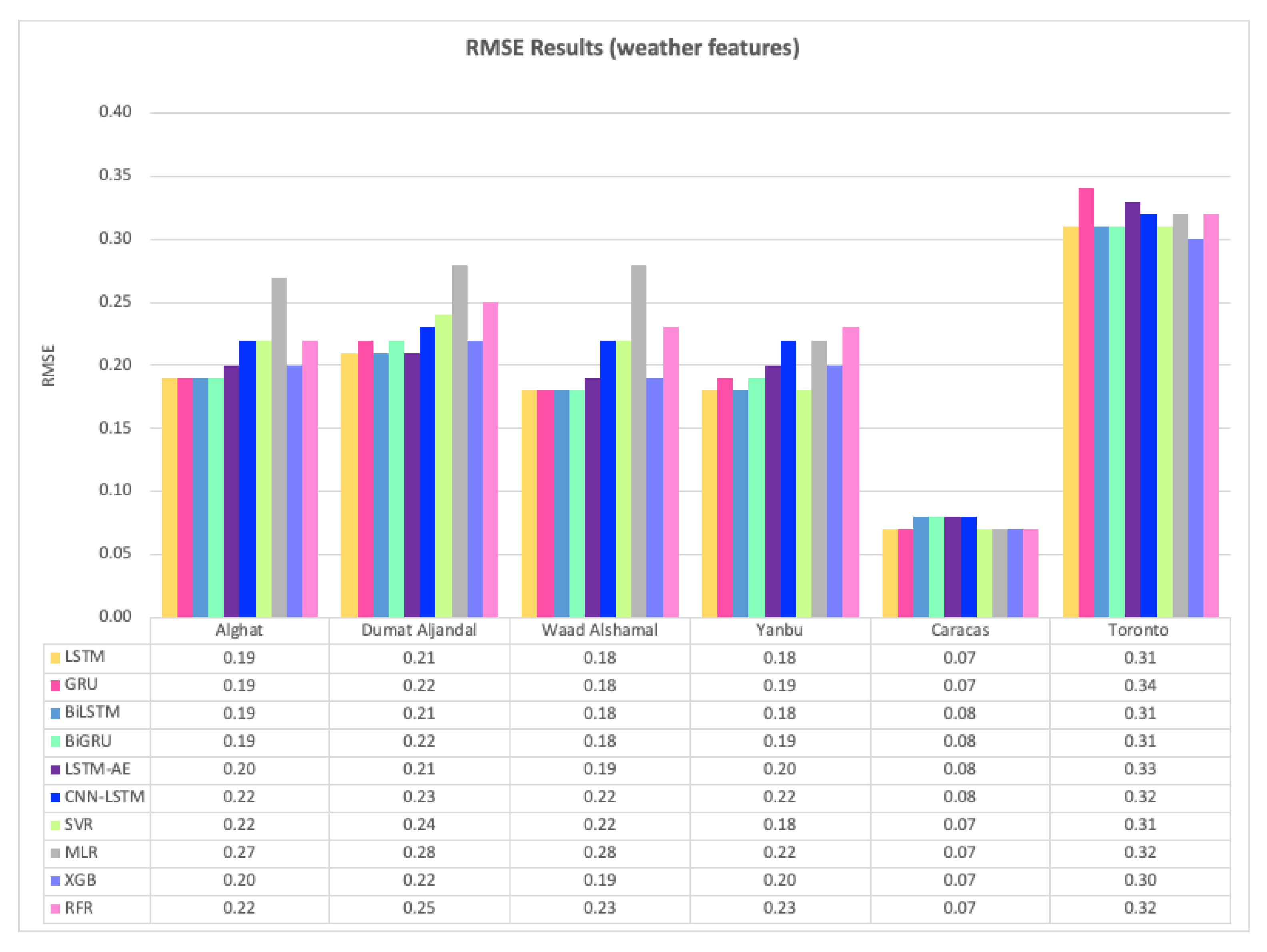
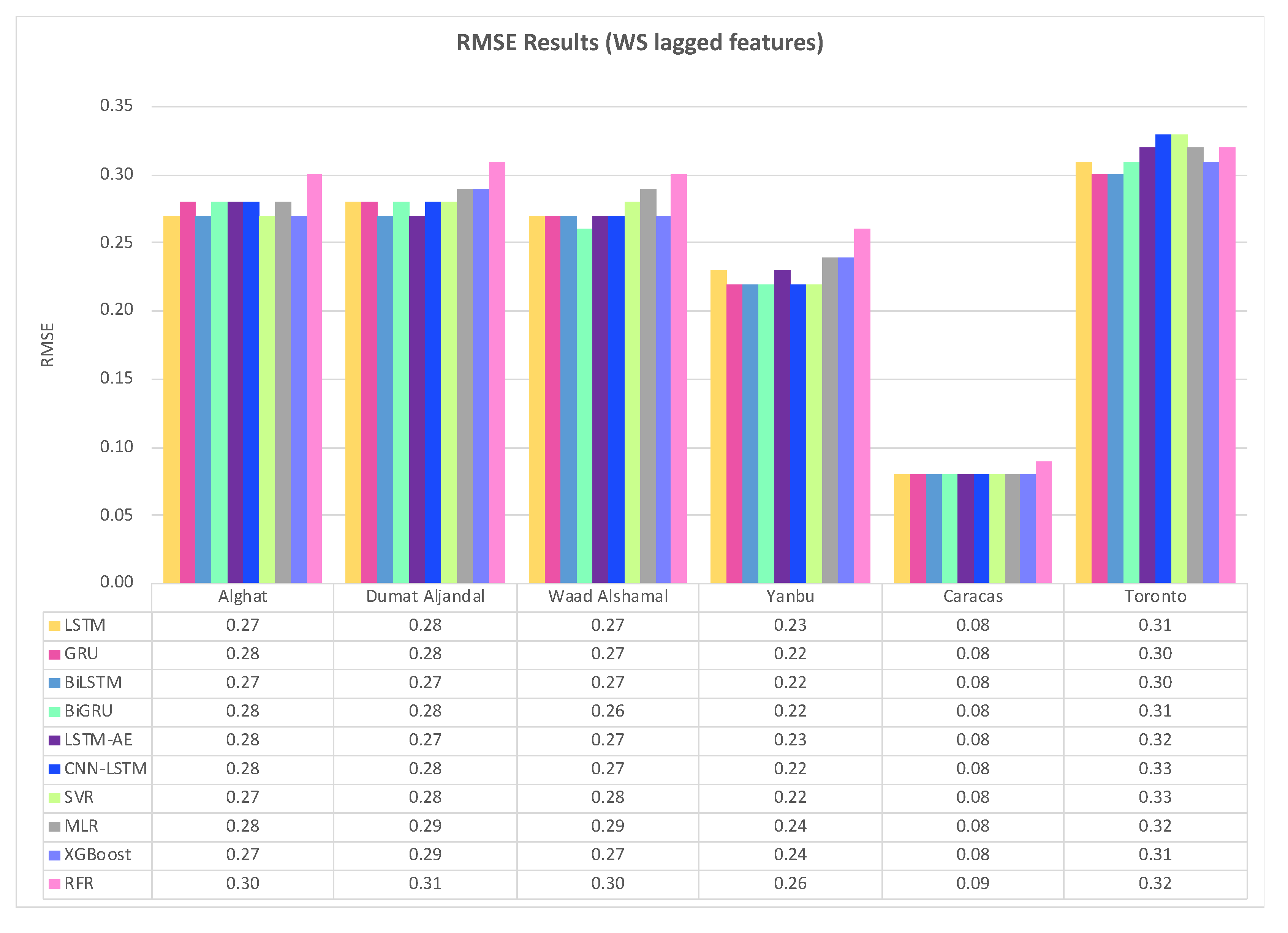
Figure 30 shows the average RMSE results of 20 runs of the six DL-based forecasting models and four ML-based models when weather features were used besides WS lagged features, whereas Figure 31 shows the same when only WS lagged features were used.
For the Alghat dataset, we noted that using weather features has improved the RMSE results for all six DL-based forecasting models by 32% at most as with GRU model and 21% at least as with CNN-LSTM model. Using weather features in ML-based models improved the RMSE results for all four models by 27% at most, as with the RFR model and 4% at least as with the MLR model. The best RMSE value is 0.19 achieved by LSTM, GRU, BiLSTM, and BiGRU models, while the worst RMSE value is 0.27 and associated with the MLR model.
For Dumat Aljandal dataset, using weather features has improved RMSE results for all six DL-based forecasting models by 25% at most as with the LSTM model and 18% at least as with the CNN-LSTM model. Using weather features in ML-based models improved the RMSE results for all four models by 24% at most as with the XGB model and 3% at least as with MLR model. The best RMSE value is 0.21 achieved by LSTM, BiLSTM, and LSTM-AE models, while the worst RMSE value is 0.28 and associated with the MLR model.
For Waad Alshamal dataset, using weather features has improved RMSE results for all six DL-based forecasting models by 33% at most as with LSTM, GRU, and BiLSTM models and 19% at least as with the CNN-LSTM model. Using weather features in ML-based models improved the RMSE results for all four models by 30% at most as with XGB model and 3% at least as with MLR model. The best RMSE value is 0.18 achieved by LSTM, GRU, BiLSTM, and BiGRU models, while the worst RMSE value is 0.28 and associated with the MLR model.
For the Yanbu dataset, using weather features has improved RMSE results for all DL-based forecasting models, except CNN-LSTM model, by 22% at most, as with the LSTM model. Using weather features in ML-based models improved the RMSE results for all four models by 18% at most, as with SVR and 8% at least as with the MLR model. The best RMSE value is 0.18 achieved by LSTM, BiLSTM, and SVR models, while the worst RMSE value is 0.23 and is associated with the RFR model.
For the Caracas dataset, using weather features has improved RMSE results only for LSTM, GRU, SVR, MLR, and XGB models by 13% and RFR model by 22% The best RMSE value is 0.07 achieved by six models with weather features.
For the Toronto dataset, using weather features has not improved the RMSE results, except for CNN-LSTM, SVR, and XGB models, which were improved by 3% at least. In fact, GRU, BiLSTM, and LSTM-AE models achieved better results with lagged features only and using weather features worsened the results. The best RMSE value is 0.30 achieved by the XGB model with weather features and achieved by GRU and BiLSTM with lagged features only.
For Saudi datasets, we can summarize RMSE results that using weather features has improved all DL-based models and ML-based models for all four locations. However, the improvement percentage is the highest with Alghat and Waad Alshamal datasets and the lowest with the Yanbu dataset. We might relate low improvement with the Yanbu dataset to the lower correlation between WS and T_lag1 and between WS and DHI_lag1 (see Figure 14) compared to other locations. Also, Yanbu is a coastal city, unlike the other three locations, and there are no significant changes in Yanbu weather from season to season. For example, the average temperature is 32° C in August and 21° C in January. With weather features, DL-based models have similar RMSE results, except CNN-LSTM model and ML-based models have similar RMSE results, except MLR model. MLR model achieved the worst RMSE value for three datasets, while LSTM and BiLSTM models attained the best RMSE value for all Saudi locations.
To summarize the RMSE results for the Caracas dataset, weather features have not improved RMSE results because WS has strong correlations with its lagged seven features (see Figure 15), which makes it easy to predict the next value with no extra features. Also, the RMSE value is 0.07 or 0.08 for all models and is a low value compared to other locations because the maximum WS in Caracas is 2.9 (see Table 6). Using weather features in the Toronto dataset has not improved RMSE results for most of the models because WS has strong correlations with its lagged twelve features (see Figure 16). Also, RMSE values for Toronto are the largest because the maximum WS is 15.6 and is the highest among all locations (see Table 6).
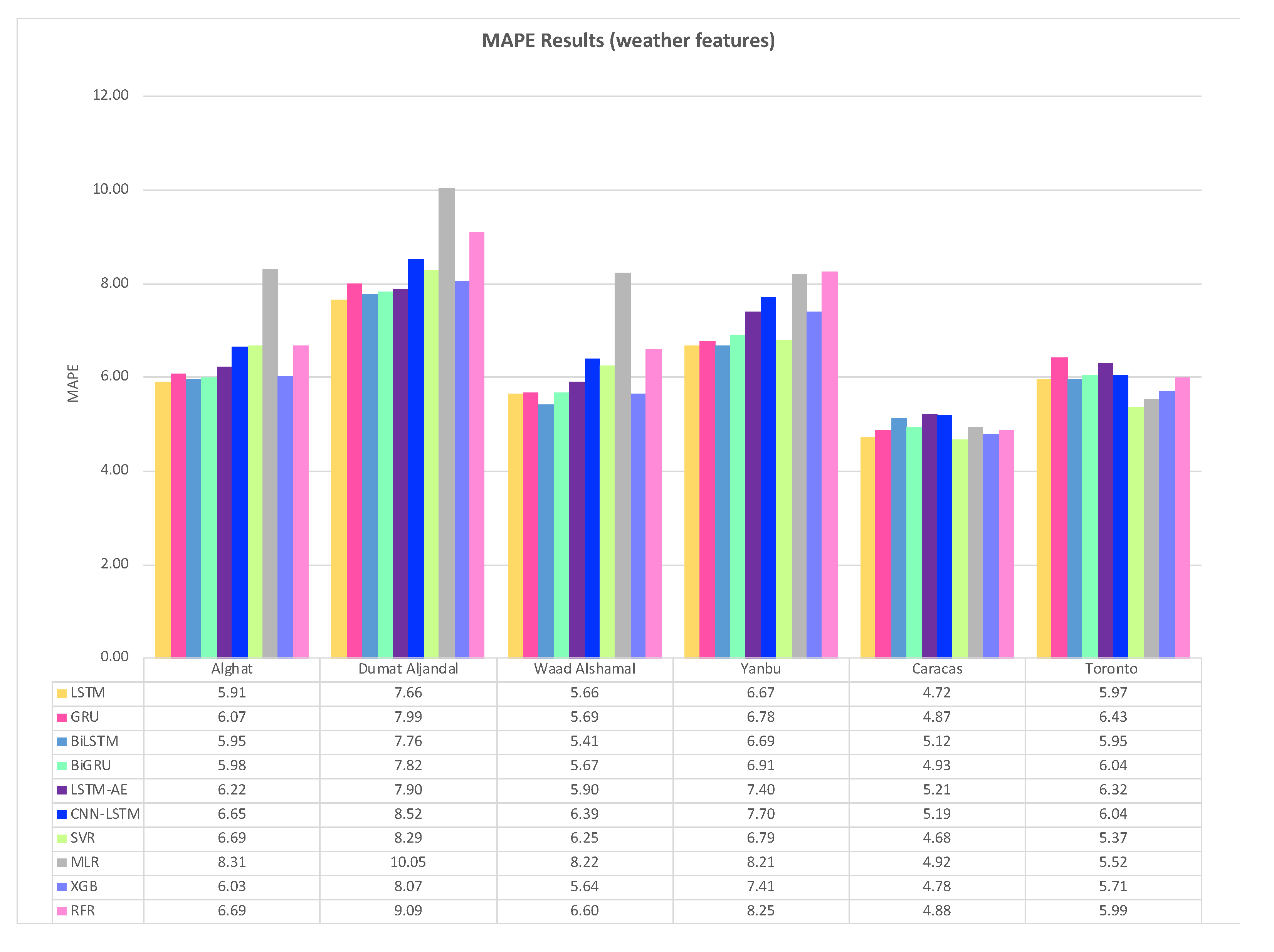
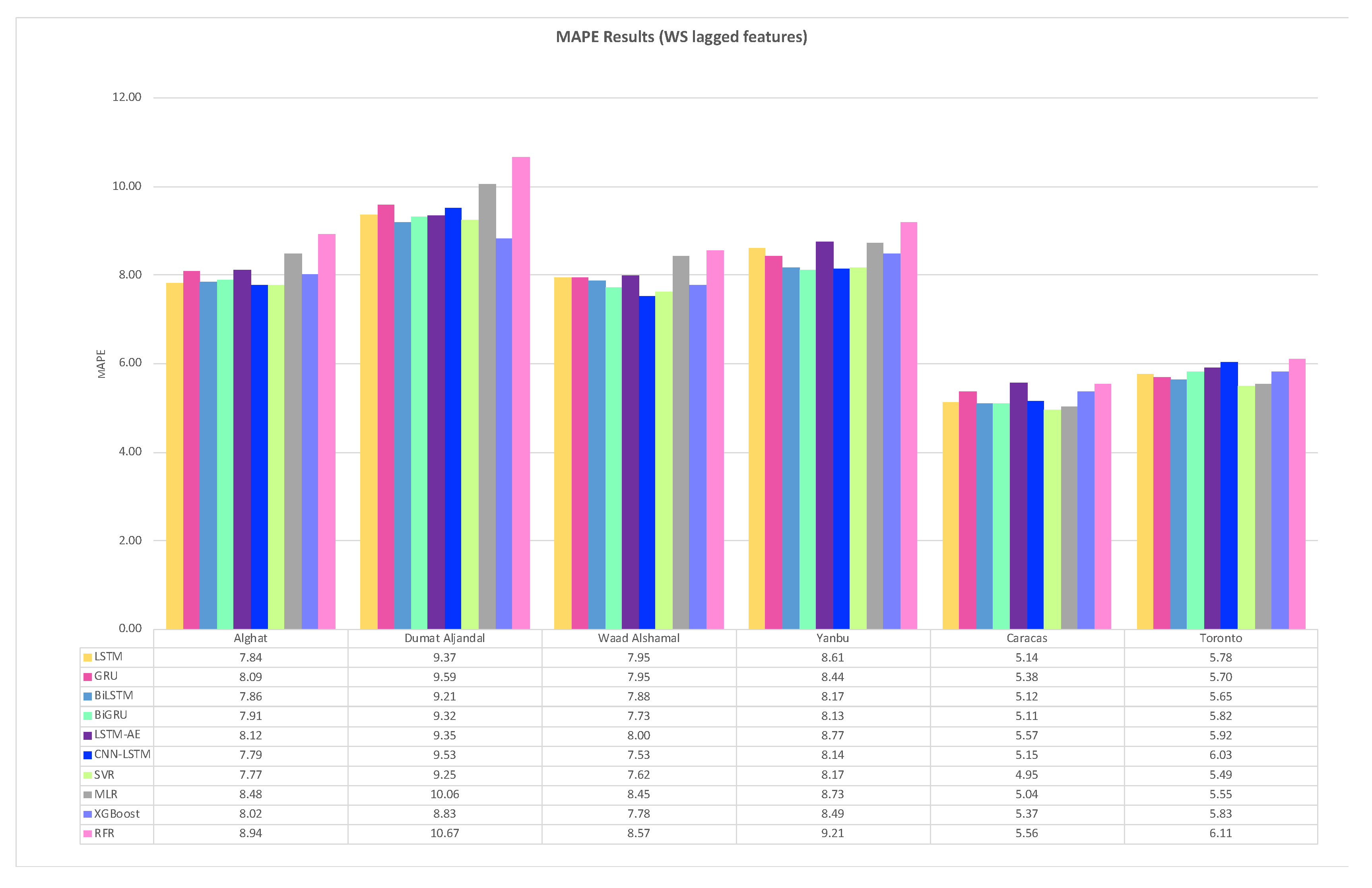
Figure 32 shows the average MAPE results of 20 runs of the six DL-based forecasting models and four ML-based models when weather features were used besides WS lagged features, whereas Figure 33 shows the same when only WS lagged features were used.
For Alghat dataset, noted that using weather features has improved the MAPE results for all six DL-based forecasting models by 25% at most as with LSTM and GRU models and 15% at least as with the CNN-LSTM model. Using weather features in ML-based models improved the RMSE results for all four models by 25% at most as with XGB and RFR models and 2% at least as with MLR model. The best MAPE value is 5.91 achieved by the LSTM model, while the worst MAPE value is 8.31 and is associated with the MLR model.
For Dumat Aljandal dataset, using weather features has improved MAPE results for all six DL-based forecasting models by 18% at most as with the LSTM model and 11% at least as with the CNN-LSTM model. Using weather features in ML-based models improved the MAPE results for the RFR model by 15% and for XGB and SVR models by 9% at least. The best MAPE value is 7.66 achieved by the LSTM model, while the worst RMSE value is 10.05 and is associated with the MLR model.
For the Waad Alshamal dataset, using weather features has improved MAPE results for all six DL-based forecasting models by 31% at most as with BiLSTM model and 15% at least as with CNN-LSTM model. Using weather features in ML-based models improved the MAPE results for all four models by 28% at most as with the XGB model and 3% at least as with MLR model. The best MAPE value is 5.41 achieved by the BiLSTM model, while the worst MAPE value is 8.22 and is associated with the MLR model.
For the Yanbu dataset, using weather features has improved MAPE results for all DL-based forecasting models by 23% at most as with the LSTM model and by 5% at least as with the CNN-LSTM model. Using weather features in ML-based models improved the MAPE results for all four models by 17% at most as with SVR and 6% at least as with the MLR model. The best MAPE value is 6.67 achieved by the LSTM model, while the worst MAPE value is 8.25 and is associated with the RFR model.
For the Caracas dataset, using weather features has improved MAPE results, except for BiLSTM and CNN-LSTM models. The highest improvement percentage is 12% for the RFR model and the lowest is 2% for the MLR model. The best MAPE value is 4.68, achieved by the SVR model with weather features.
For the Toronto dataset, using weather features has not improved MAPE results, except for ML-based models, which were improved by 2% at most. In fact, DL-based models achieved better results with lagged features only and using weather features worsened the results. The best MAPE value is 5.37, achieved by the SVR model with weather features.
For Saudi datasets, we can summarize MAPE results that using weather features has improved all DL- and ML-based models for all four locations. However, the improvement percentage is the highest with the Alghat and Waad Alshamal datasets and the lowest with the Yanbu dataset. We might relate low improvement with the Yanbu dataset to the lower correlation between WS and T_lag1 and between WS and DHI_lag1 (see Figure 14) compared to other locations. Also, Yanbu is a coastal city, unlike the other three locations, and there are no significant changes in Yanbu weather from season to season. For example, the average temperature is 32° C in August and 21° C in January. With weather features, all models have similar MAPE results, except MLR and RFR models. MLR model achieved the worst MAPE value for three datasets, while LSTM attained the best MAPE value for three datasets out of four Saudi locations.
To summarize MAPE results for the Caracas dataset, weather features have improved MAPE results because WS has strong correlations with its lagged seven features (see Figure 15), which makes it easy to predict the next value with no extra features. Using weather features in the Toronto dataset has not improved MAPE results for most of the models because WS has strong correlations with its lagged twelve features (see Figure 16).
From MAE, RMSE, and MAPE results in this section, we note that using weather features has improved the forecasting results of all models for Saudi locations by around 30% at most. However, DL-based models experienced higher improvement than ML-based models did. This may be related to DL-based models’ ability to handle high dimensionality. Also, the Yanbu dataset has the least improvement percentage because, as explained earlier, Yanbu is a coastal city, unlike the other three locations, and there are no significant changes in Yanbu weather from season to season. This makes weather features less important than WS lagged features in predicting the next value of WS. This is reflected in the lower correlation between WS and T_lag1 and between WS and DHI_lag1 (see Figure 14) compared to other locations. Weather features with Caracas improved the forecasting results slightly, while it has worsened the results with Toronto for most of the models. The reason behind this is strong WS correlations with its lagged features. We used seven lagged features for Caracas and twelve for Toronto (see Figure 10). Therefore, the results of ML-based models are better or similar to the results of DL-based models for both locations. We can conclude that when wind speed has strong correlations with its lagged values, ML-based models’ performance would be satisfactory (i.e., SVR and XGB models) while DL-based models are needed with less strong or weak correlations. The same applies to weather features, which can improve the forecasting results more if there are less strong correlations between WS and its lagged features.

4.2. Effect of Seasonality on Forecasting

The datasets used in this work cover the period from January 2017 to December 2019. As mentioned earlier in Section 3.1.3, we used 15% of the size of the datasets for testing, hence; the testing set starts from July 20 to December 31, 2019, and it only contains complete data for the last five months of the year 2019. In this section, we present the changes in MAE, RMSE, and MAPE for August, September, October, November, and December to note the effect of seasonality on next-hour WS forecasting.
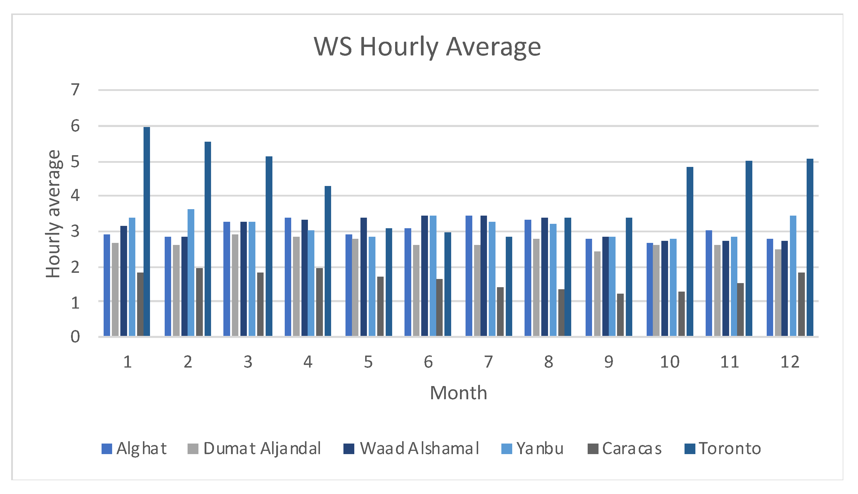
Figure 34 shows the WS hourly average per month for all datasets. Saudi Arabia has only two seasons and, as shown in the figure, the WS hourly average does not differ from month to month, which ranges from 2.42 to 3.6 m/s. In Alghat, the WS hourly average is above 3 m/s in March, April, June, July, August, and November, whereas in Dumat Aljandal, it has not reached 3 m/s. In Yanbu, the WS hourly average is above 3 m/s in all months, except May, September, October, and November. Among the Saudi locations, Yanbu has the highest average and Dumat Aljandal has the lowest. As noted in [47], the western region of Saudi Arabia, where Yanbu is located, has more potential for wind energy than other regions do. In Caracas, the WS hourly average is low compared to other locations and the highest value is 1.94 m/s in February. It drops below 1.5 from July to October. In contrast, the WS hourly average in Toronto is high compared to other locations and the highest value is 5.95 m/s in January. It drops below 4 from May to September.
Figure 35 shows MAE, RMSE, and MAPE results for five months (August, September, October, November, and December) for all datasets. Alghat results (a) and (b) show that according to MAE and RMSE results of all models, November and December results are worse than the remaining months, except for the MLR model, which performs worse in August and December. MAPE results of all models as shown in (c) show that October has the worst results followed by November and December. Dumat Aljandal's results in (d), (e), and (f), show October results are the worst for all models. For Waad Alshamal results in (g) and (h), October results are the worst for all models, except for the MLR model whereas MAPE results in (i) show that December besides October has the worst results. Yanbu results in (g), (k), and (l), show performance differences across months from model to model. However, September and October have higher errors than other months for most of the models. Caracas results in (m), (n), and (o) show that September is the most difficult month for forecasting. Toronto MAE results in (p) show that October and December have the highest error, while RMSE results in (q) show a significant increase in October error. Toronto MAPE results in (r) show that August and September results are even worse than October.
To conclude, it is unnecessary to worry about seasonality effects unless the hourly average of WS varies from one month to another or from one season to another. In the Saudi locations covered, there is no significant variance in the results from August to December, despite higher errors in some months, such as October. However, longer testing sets that cover a whole year should validate this observation. Caracas has the lowest WS hourly average in September. It also has the highest forecasting error. In Toronto, MAPE results show the same inverse relationship in which August and September have the lowest WS hourly average and the highest forecasting error. However, we cannot validate this observation without a test set covering a whole year.

4.3. Effect of Using Decomposition Methods on Forecasting

To study this effect, three decomposition methods (described in Section 3.1.4) are combined with the LSTM model. Section 3.2.1.6. describes the structure of these hybrid models in detail. The features used to train and test the three hybrid models are the last five hours’ WS values in Saudi locations, the last seven values in Caracas, and the last twelve values in Toronto. The forecasting results of the three hybrid models are compared to six DL-based models and four ML-based models (the same results appeared in Section 4.1 for WS lagged features in Figure 29, Figure 31, and Figure 33).
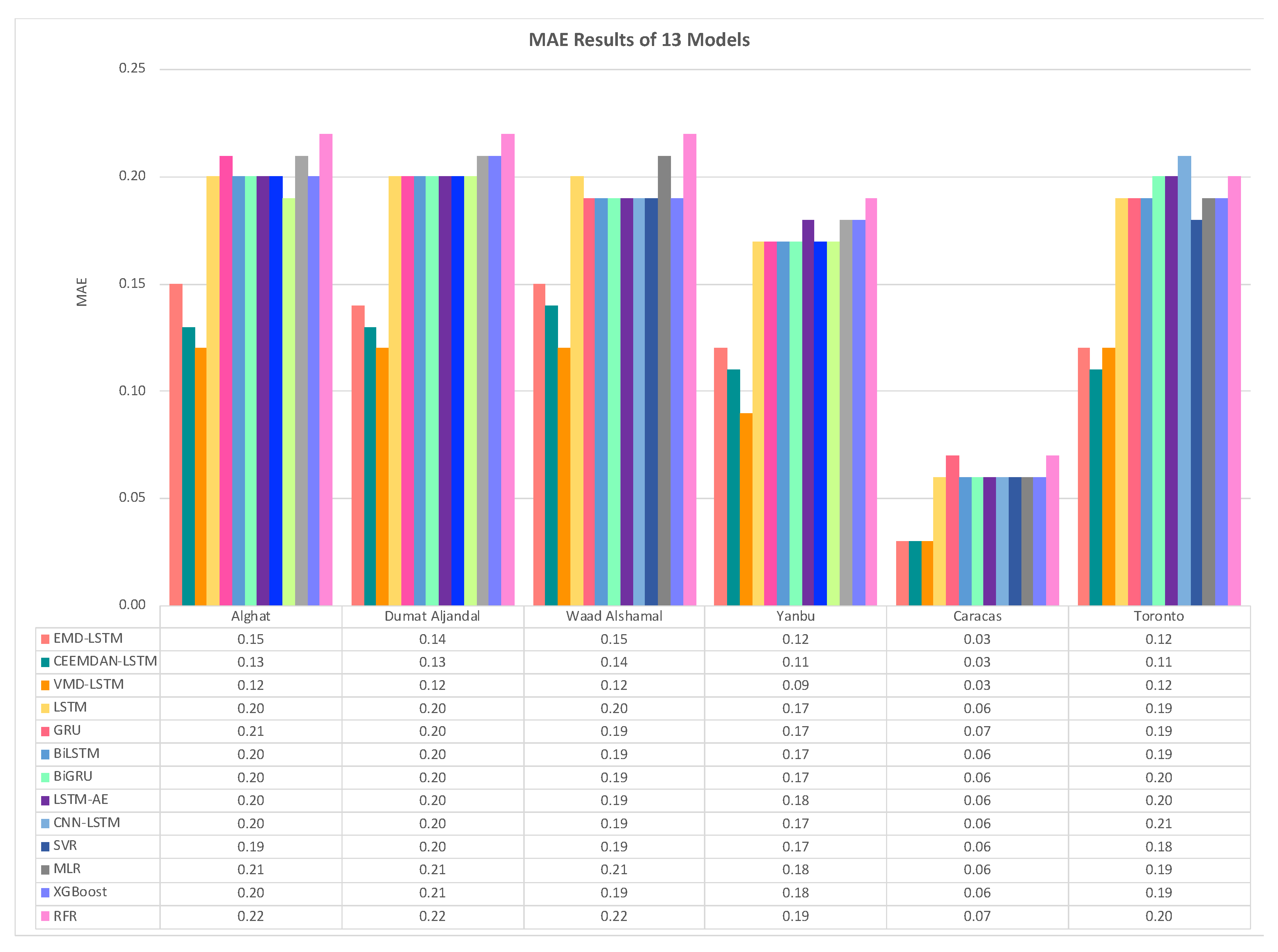
Figure 36 shows the MAE results of three hybrid models (EMD-LSTM, CEEMDAN-LSTM, VMD-LSTM), six DL-based models (LSTM, GRU, BiLSTM, BiGRU, LSTM-AE, CNN-LSTM), and four ML-based models (SVR, MLR, XGB, RFR) for all datasets.
From Figure 36, we note that the best performing model for all Saudi locations is VMD-LSTM model, and the worst is RFR model. The hybrid model of VMD-LSTM achieved MAE value equals to 0.12, which improved the forecasting results over LSTM model by 40% for Alghat, Dumat Aljandal, and Waad Alshamal. It also achieved MAE value equals to 0.09 for Yanbu, which improved the forecasting results over the LSTM model by 47%. Regarding the Caracas dataset, all three hybrid models achieved the same MAE value equals to 0.03, which provided 50% improvement over the LSTM model result. With the Toronto dataset, the hybrid model of CEEMDAN-LSTM achieved better MAE value than the other two hybrid models, which provided 42% improvement over the LSTM model result.
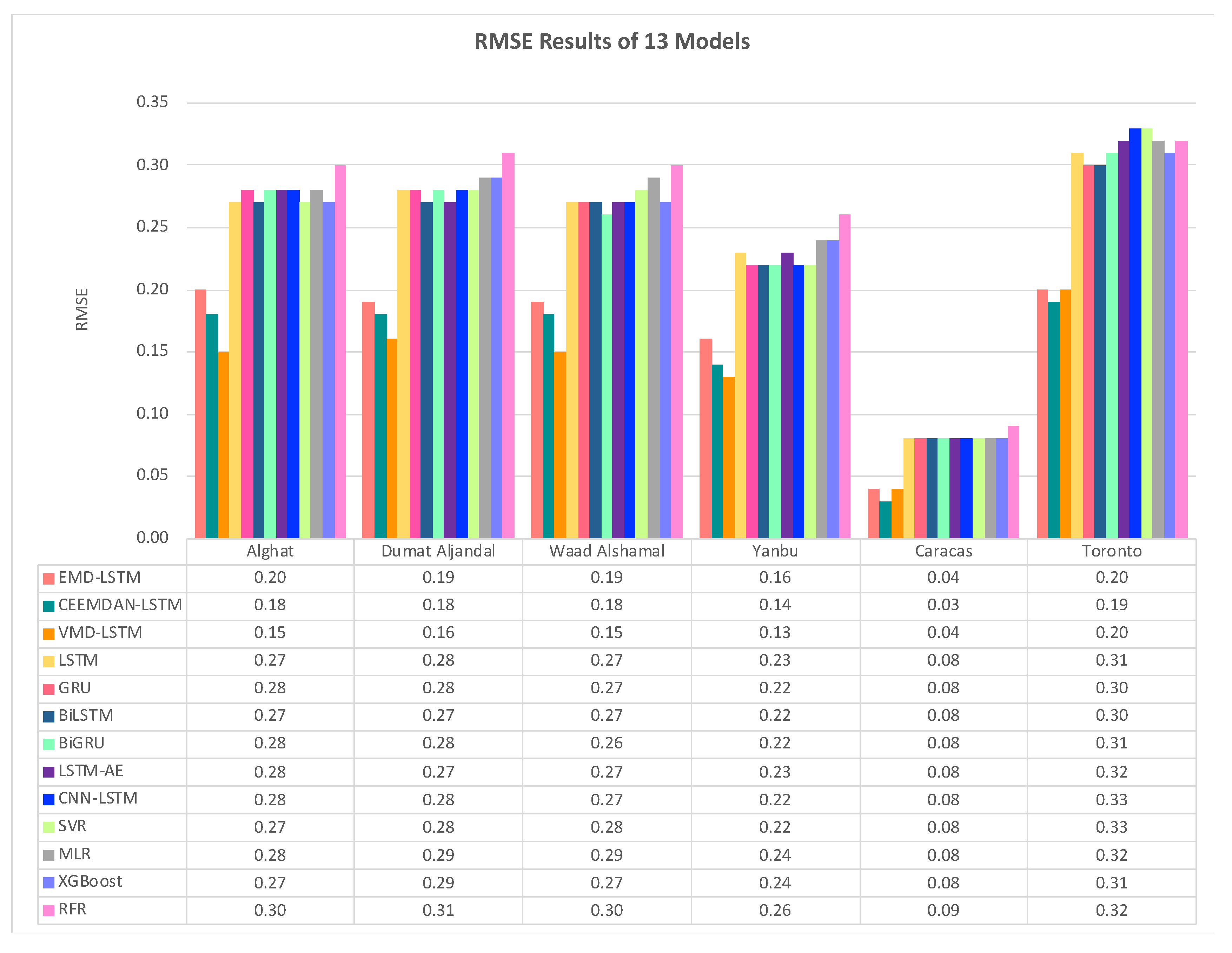
Figure 37 shows the RMSE results of three hybrid models (EMD-LSTM, CEEMDAN-LSTM, VMD-LSTM), six DL-based models (LSTM, GRU, BiLSTM, BiGRU, LSTM-AE, CNN-LSTM), and four ML-based models (SVR, MLR, XGB, RFR) for all datasets.
From Figure 37, we note that the best performing model for all Saudi locations is the VMD-LSTM model, and the worst is the RFR model. The hybrid model of VMD-LSTM achieved RMSE value equals to 0.15, which improved the forecasting results over LSTM model by 44% for Alghat and Waad Alshamal. It also achieved RMSE value equals to 0.16 for Dumat Aljandal and 0.13 for Yanbu, which improved the forecasting results over LSTM model by 43%. Regarding the Caracas and the Toronto datasets, the hybrid model of CEEMDAN-LSTM achieved slightly better RMSE value than the other two hybrid models, which considered 63% improvement in Caracas and 39% improvement in Toronto forecasting results over LSTM model.
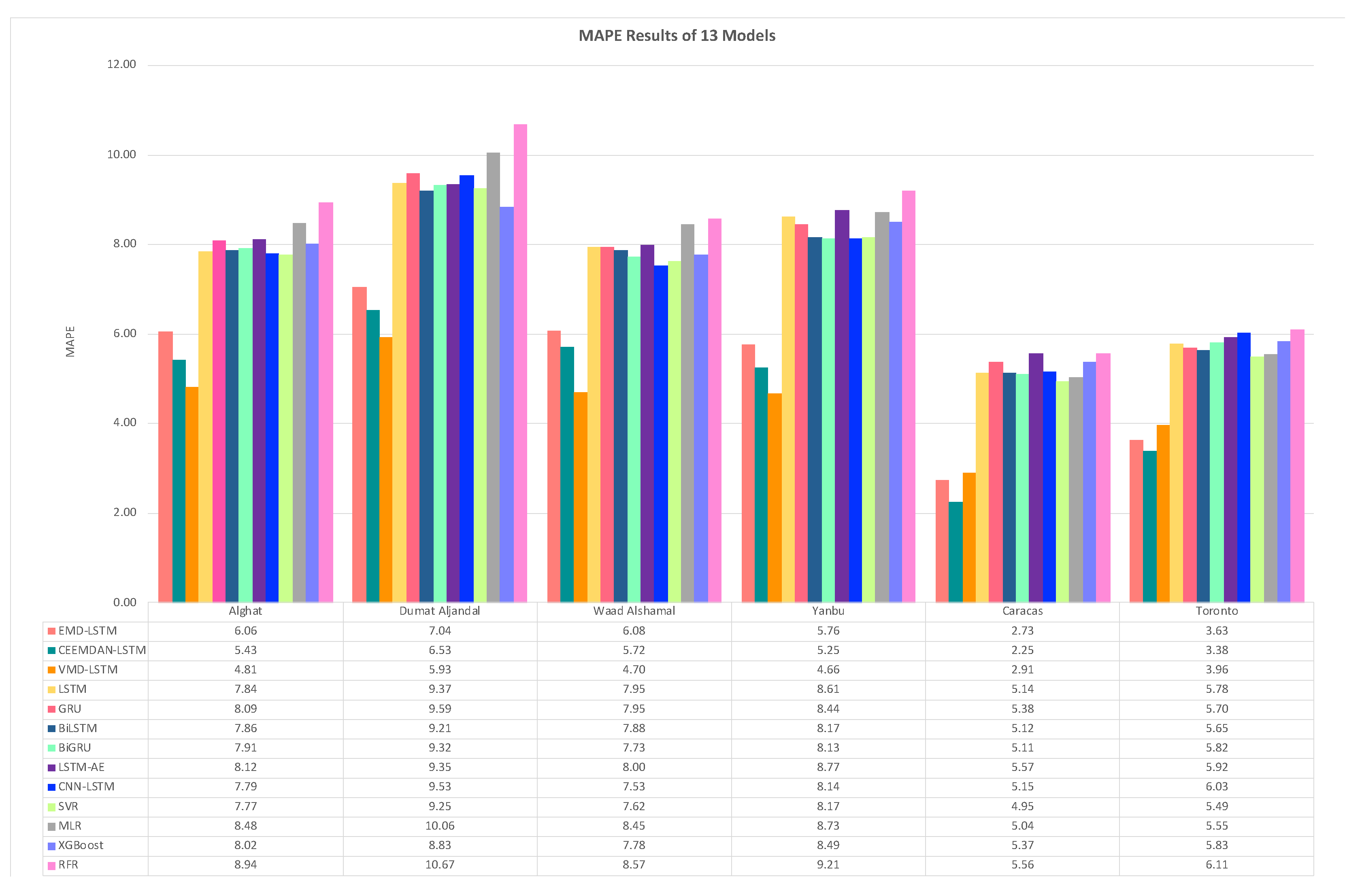
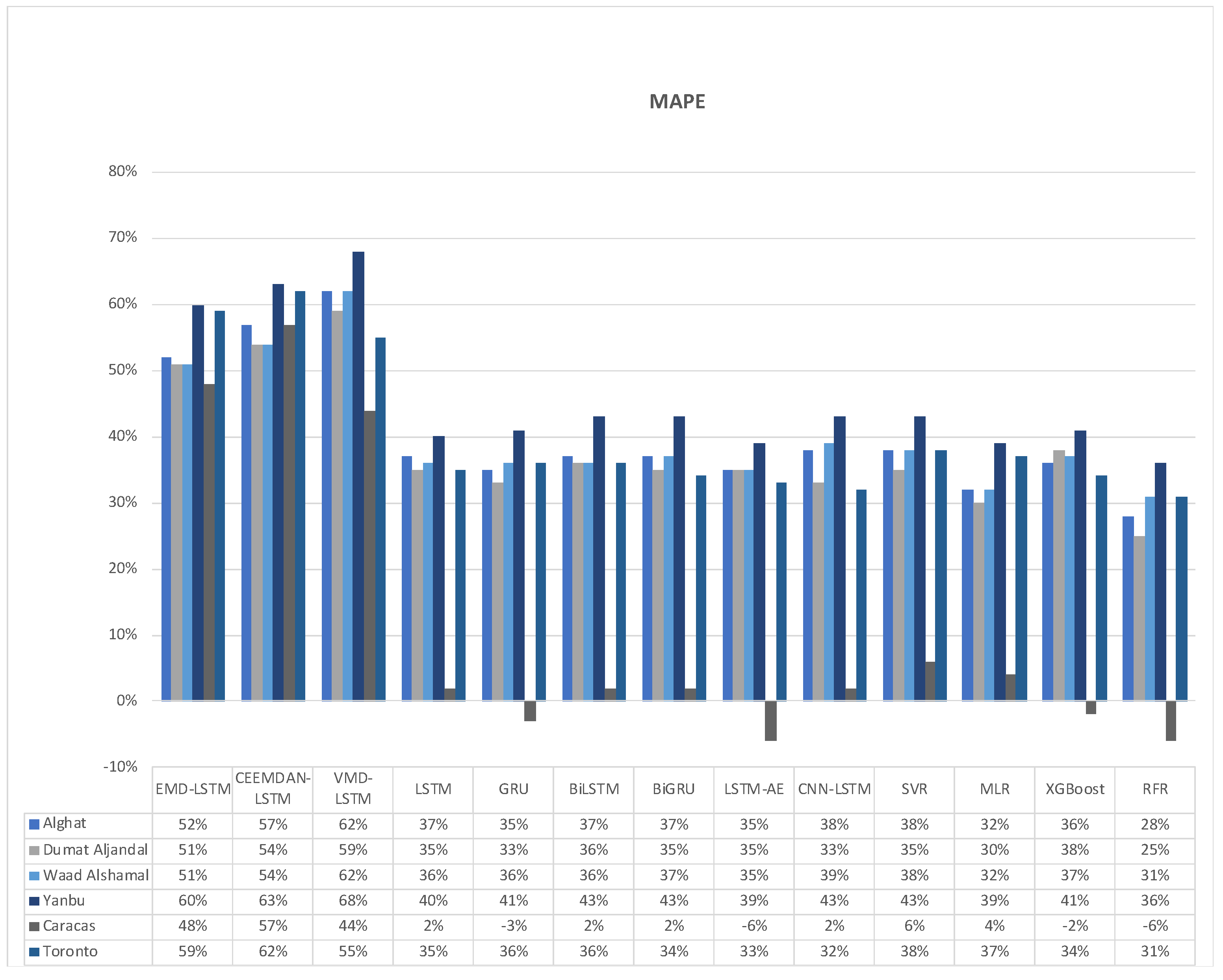
Figure 38 shows the MAPE results of three hybrid models (EMD-LSTM, CEEMDAN-LSTM, VMD-LSTM), six DL-based models (LSTM, GRU, BiLSTM, BiGRU, LSTM-AE, CNN-LSTM), and four ML-based models (SVR, MLR, XGB, RFR) for all datasets.
From Figure 38, we note that the best performing model for all Saudi locations is the VMD-LSTM model, and the worst is the RFR model. The hybrid model of VMD-LSTM achieved MAPE value equals to 4.81 for Alghat and 5.39 for Dumat Aljandal, which improved the forecasting results over the LSTM model by 39% and 37% for both locations. It also achieved MAPE value equals to 4.7 for Waad Alshamal and 4.66 for Yanbu, which improved the forecasting results over the LSTM model by 41% and 46% for both locations. Regarding the Caracas and the Toronto datasets, the hybrid model of CEEMDAN-LSTM achieved better MAPE value than the other two hybrid models, which considered 58% improvement in Caracas and 41% improvement in Toronto forecasting results over the LSTM model.
From MAE, RMSE, and MAPE results in this section, we conclude that using a hybrid model of LSTM and a decomposition method always achieves better results than using the LSTM model alone. In Saudi locations, the best hybrid model is VMD-LSTM according to all evaluation metrics, with improvement percentage ranges from 39% to 47% over the LSTM model. This observation agrees with the performance comparison done in [29] between EMD, Ensemble EMD, Wavelet Packet Decomposition, and VMD, in which VMD achieved the most accurate and stable performance. Also, in [48], VMD compared well to Empirical Wavelet Transform, Complementary Ensemble Empirical Mode Decomposition, and Ensemble Intrinsic Time-scale Decomposition. VMD outperformed EMD in [49]. In this field, many works show that VMD-based models perform better compared with Wavelet Transform-based and EMD-based models [29,50,51]. The reason behind the VMD superiority is its ability to decompose nonstationary and nonlinear time series and its robustness handling data noise.
Regarding the Caracas and the Toronto datasets, the best hybrid model is CEEMDAN-LSTM according to all evaluation metrics with improvement percentage ranges from 50% to 63% over LSTM model in Caracas and from 39% to 42% over LSTM model in Toronto.
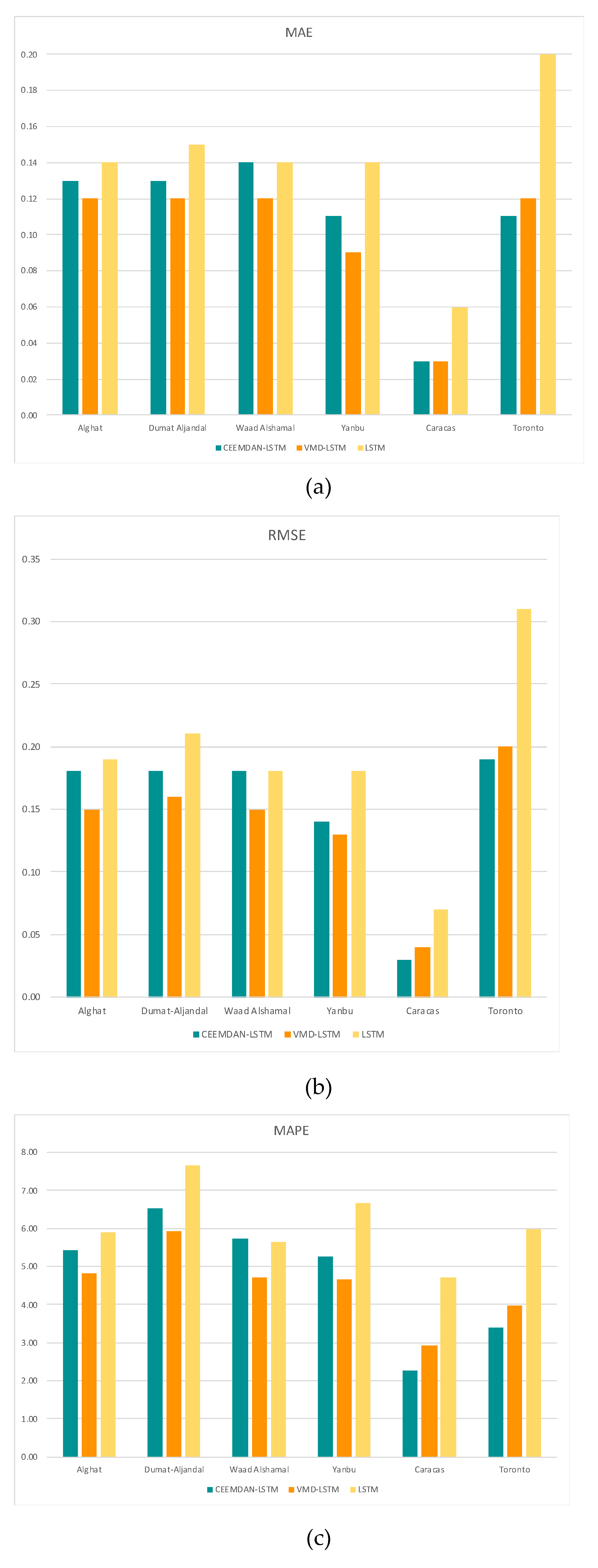
We studied decomposition methods for forecasting by comparing the results of hybrid models to the results of DL- and ML-based models using only lagged WS values. We wonder which method is better: hybrid models with decomposition methods or weather variables with DL-based models (as done in Section 4.1). To answer this question, we compared the best performing hybrid models VMD-LSTM and CEEMDAN-LSTM to the LSTM model that was trained and tested using weather variables for each dataset in Figure 39. Figure 39 (a) shows MAE results for these three models, while RMSE and MAPE results are shown in (b) and (c). From the figure, we can see that the VMD-LSTM model achieved the best forecasting accuracy for Saudi datasets, while the CEEMDAN-LSTM model achieved the same for Caracas and Toronto datasets. Therefore, we can conclude that hybrid models with decomposition methods achieved better results than using weather variables with DL-based models.

4.4. Forecast Skills of all Models

We compared DL-based model performance to ML-based models and hybrid models with decomposition methods. In this section, the forecast skills of all forecasting models are presented, which measure the improvement in forecasting compared to the persistence method. This metric (refer to equation 7) not only shows the feasibility of a proposed model for the same dataset but also helps to evaluate a model's performance compared to other models developed using different datasets. The results presented in this section are for the forecasting models that were trained and tested using WS lagged features.
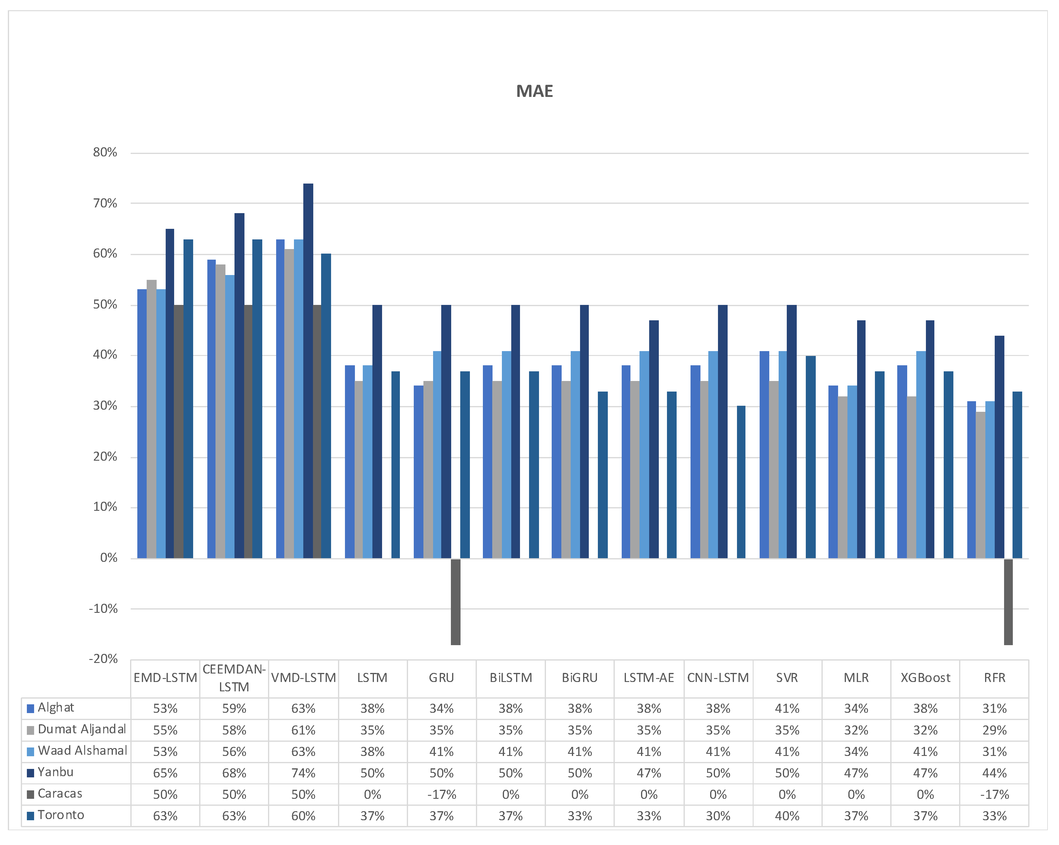
Figure 40 shows the FS of all models using the MAE metric for all six datasets. From the figure, we note that the highest FS values for Saudi datasets are achieved by the VMD-LSTM model, and the worst are associated with the RFR model. For Caracas, only the three hybrid models achieved improvement over the persistence method by 50%. For Toronto, the EMD-LSTM model and CEEMDAN-LSTM model attained 63% as the highest FS value, whereas the worst was 30% associated with the CNN-LSTM model.
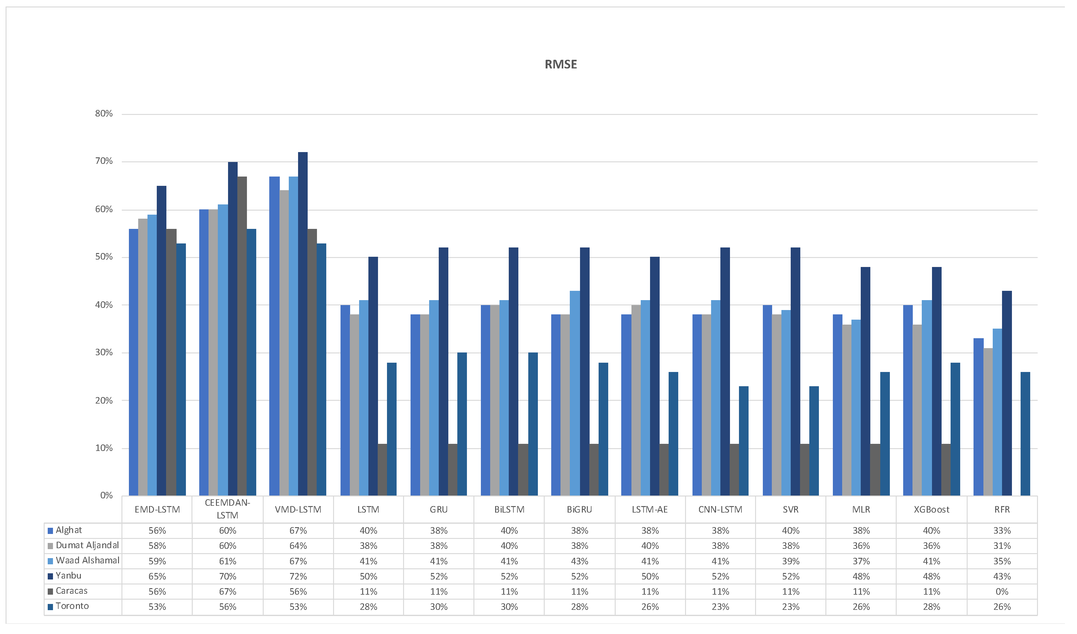
Figure 41 shows the FS of all models using the RMSE metric for all six datasets. From the figure, we note that the highest FS values for Saudi datasets are achieved by the VMD-LSTM model, and the worst are associated with the RFR model. For Caracas, the CEEMDAN-LSTM model achieved the best FS of 67%. The remaining two hybrid models attained FS equal to 56% while other models could not improve the FS by more than 11%. For Toronto, the CEEMDAN-LSTM model attained 56% as the highest FS value, whereas the worst was 23%, associated with CNN-LSTM and SVR models.
Figure 42 shows the FS of all models using the MAPE metric for all six datasets. From the figure, we note that the highest FS values for Saudi datasets are achieved by the VMD-LSTM model, and the worst are associated with the RFR model. For Caracas, the CEEMDAN-LSTM model achieved the best FS equal to 57%. The remaining two hybrid models attained FS equal to 48% and 44%, while most of the remaining models are worse than the persistence method. For Toronto, the CEEMDAN-LSTM model attained 62% as the highest FS value, whereas the worst was 31%, associated with the RFR model.
We conclude from the figures above that the highest FS percentages of all metrics are achieved by hybrid models. The VMD-LSTM model is the best with the Saudi datasets, and the CEEMDAN-LSTM model is the best with the Caracas and Toronto datasets. Also, apart from the hybrid models for Caracas, other models are worse, equal to, or just better than, the persistence method. The significant correlation between WS and its last value in Caracas makes prediction with the persistence method easier and more accurate.

5. Conclusion

This paper aims to propose a novel hybrid model that combines VMD and LSTM that is developed for next-hour wind speed prediction in a hot desert climate, such as the climate in Saudi Arabia. It also shows the improvement in the accuracy of DL models over ML with and without exogenous variables to give insights about important data features. It highlights the performance gain of hybrid models over single models to justify the added complexity and help in making an informed decision about the tradeoff between accuracy and efficiency. These objectives are achieved through the performance comparison of three hybrid models, six DL-based models, and four ML-based models, which cover several aspects, such as seasonality and using different features and decomposition methods.
We can summarize the findings:
  • The best forecasting model for the Saudi locations, according to MAE, RMSE, MAPE, and FS, is the hybrid model of VMD and LSTM model.
  • The best forecasting model for Caracas and Toronto, according to MAE, RMSE, MAPE, and FS, is the hybrid model of CEEMDAN and the LSTM model.
  • All DL-based models have similar performance, but complex structures like the LSTM-AE and CNN-LSTM models have higher errors.
  • Using the last hour’s weather variables besides the last values of WS has improved the forecasting results for all models. However, the hybrid models with decomposition methods achieved better forecasting results.
  • If seasons do not affect the hourly average of WS at the data source location, forecasting results would not show a big variance either. Here, it is unnecessary to partition the datasets according to seasons and train separate forecasters.
In future work, we will build a novel DL-based auto-selective approach and tool that predicts the best-performing DL model for wind energy forecasting, as we did in [52] for solar energy. Also, the datasets used were collected by satellite from the NSRDB website and only covered three years. We could not find complete ground-based data for the desired locations and periods. In the future, we will try to find accurate ground-based data for a longer period and more locations to validate the results.

Author Contributions

Conceptualization, G.A. and R.M.; methodology, G.A. and R.M.; software, G.A.; validation, G.A. and R.M.; formal analysis, G.A., R.M. and S.H.H.; investigation, G.A., R.M. and S.H.H.; resources, G.A., R.M. and S.H.H.; data curation, G.A.; writing—original draft preparation, G.A. and R.M.; writing—review and editing, R.M. and S.H.H.; visualization, G.A.; supervision, R.M. and S.H.H. All authors have read and agreed to the published version of the manuscript.

Funding

This research received no external funding.

Data Availability Statement

We have provided details about the sources of data in the manuscript.

Conflicts of Interest

The authors declare no conflict of interest.

Abbreviations

SA Saudi Arabia
NWP Numerical Weather Prediction
RNN Recurrent Neural Network
kNN K-Nearest Neighbors
AE Autoencoder
LSTM Long Short-Term Memory
CNN Convolutional Neural Network
GRU Gated Recurrent Unit
BiLSTM Bidirectional LSTM
BiGRU Bidirectional GRU
RFR Random Forest Regression
MLR Multiple Linear Regression
MLP Multilayer Perceptron Network
VMD Variational Mode Decomposition
EMD Empirical Mode Decomposition
CEEMDAN Complete Ensemble Empirical Mode Decomposition with Adaptive Noise
SVR Support Vector Regression
RMSE Root Mean Square Error
MAPE Mean Absolute Percentage Error
MAE Mean Absolute Error
MSE Mean Squared Error loss
WS Wind Speed
WD Wind Direction
WP Wind Power
T Temperature
P Pressure
RH Relative Humidity
ZA Zenith Angle
PW Precipitable Water
DP Dew Point
HS Hour Sine
HC Hour Cosine
DS Day Sine
DC Day Cosine
WDS Wind Direction Sine
WDC Wind Direction Cosine
ML Machine Learning
DL Deep Learning
FFNN Feed Forward Neural Network
GHI Global Horizontal Irradiation
DHI Diffuse Horizontal Irradiation
DNI Direct Normal Irradiance
WSTD Wavelet Soft Threshold Denoising
ReLU Rectified Linear Unit
RR Ridge Regression
ESN Echo State Network
PE Permutation Entropy
RBFNN Radial Basis Function Neural Network
IBA Improved Bat Algorithm
FS Forecast Skill
XGB eXtreme Gradient Boosting
ACF Autocorrelation Function
GA Genetic Algorithm
LN Linear-Nonlinear
MOBBSA Multi-Objective Binary Back-tracking Search Algorithm
DE Differential Evolution algorithm
SIRAE Stacked Independently Recurrent Auto Encoder
NSRDB National Solar Radiation Data Base
NREL National Renewable Energy Laboratory
PSM Physical Solar Model
SD Standard Deviation
VAR Variance
IMFs Intrinsic Mode Functions
ARIMA Auto Regressive Integrated Moving Average

References

  1. International Renewable Energy Agency (IRENA), “Future of Wind - Executive Summary,” 2019.
  2. Dumat Al Jandal wind farm in Saudi Arabia starts production. Available online: https://www.power-technology.com/news/dumat-al-jandal-wind/ (accessed on 24 February 2023).
  3. Giani, P.; Tagle, F.; Genton, M.G.; Castruccio, S.; Crippa, P. Closing the gap between wind energy targets and implementation for emerging countries. Appl. Energy 2020, 269, 115085. [Google Scholar] [CrossRef]
  4. Alharbi, F.; Csala, D. Saudi Arabia’s Solar and Wind Energy Penetration: Future Performance and Requirements. Energies 2020, 13, 588. [Google Scholar] [CrossRef]
  5. Saudi press agency, “Saudi Arabia Announces Floating Five Projects to Produce Electricity with Use of Renewable Energy with Total Capacity of 3,300mw,” 25/09/2022. Available online: https://www.spa.gov.sa/viewfullstory.php?lang=en&newsid=2386966 (accessed on 1 April 2023).
  6. Mohandes, M.A.; Rehman, S. Wind Speed Extrapolation Using Machine Learning Methods and LiDAR Measurements. IEEE Access 2018, 6, 77634–77642. [Google Scholar] [CrossRef]
  7. Abualigah, L.; Abu Zitar, R.; Almotairi, K.H.; Hussein, A.M.; Elaziz, M.A.; Nikoo, M.R.; Gandomi, A.H. Wind, Solar, and Photovoltaic Renewable Energy Systems with and without Energy Storage Optimization: A Survey of Advanced Machine Learning and Deep Learning Techniques. Energies 2022, 15, 578. [Google Scholar] [CrossRef]
  8. V. Bali, A. Kumar, and S. Gangwar, “Deep learning based wind speed forecasting-A review,” in 2019 9th International Conference on Cloud Computing, Data Science & Engineering (Confluence), 2019, pp. 426–431.
  9. Deng, X.; Shao, H.; Hu, C.; Jiang, D.; Jiang, Y. Wind Power Forecasting Methods Based on Deep Learning: A Survey. Comput. Model. Eng. Sci. 2020, 122, 273–301. [Google Scholar] [CrossRef]
  10. Liu, H.; Chen, C.; Lv, X.; Wu, X.; Liu, M. Deterministic wind energy forecasting: A review of intelligent predictors and auxiliary methods. Energy Convers. Manag. 2019, 195, 328–345. [Google Scholar] [CrossRef]
  11. Alkhayat, G.; Mehmood, R. A review and taxonomy of wind and solar energy forecasting methods based on deep learning. Energy AI 2021, 4, 100060. [Google Scholar] [CrossRef]
  12. Manero, J.; Béjar, J.; Cortés, U. “Dust in the Wind...”, Deep Learning Application to Wind Energy Time Series Forecasting. Energies 2019, 12, 2385. [Google Scholar] [CrossRef]
  13. Peng, Z.; Peng, S.; Fu, L.; Lu, B.; Tang, J.; Wang, K.; Li, W. A novel deep learning ensemble model with data denoising for short-term wind speed forecasting. Energy Convers. Manag. 2020, 207, 112524. [Google Scholar] [CrossRef]
  14. Alhussein, M.; Haider, S.I.; Aurangzeb, K. Microgrid-Level Energy Management Approach Based on Short-Term Forecasting of Wind Speed and Solar Irradiance. Energies 2019, 12, 1487. [Google Scholar] [CrossRef]
  15. Lawal, A.; Rehman, S.; Alhems, L.M.; Alam, M. Wind Speed Prediction Using Hybrid 1D CNN and BLSTM Network. IEEE Access 2021, 9, 156672–156679. [Google Scholar] [CrossRef]
  16. Faniband, Y.P.; Shaahid, S.M. Univariate Time Series Prediction of Wind speed with a case study of Yanbu, Saudi Arabia. Int. J. 2021, 10, 257–264. [Google Scholar]
  17. Zheng, Y.; Ge, Y.; Muhsen, S.; Wang, S.; Elkamchouchi, D.H.; Ali, E.; Ali, H.E. New ridge regression, artificial neural networks and support vector machine for wind speed prediction. Adv. Eng. Softw. 2023, 179, 103426. [Google Scholar] [CrossRef]
  18. Salman, U.T.; Rehman, S.; Alawode, B.; Alhems, L.M. Short term prediction of wind speed based on long-short term memory networks. FME Trans. 2021, 49, 643–652. [Google Scholar] [CrossRef]
  19. Huang, H.; Castruccio, S.; Genton, M.G. Forecasting High-Frequency Spatio-Temporal Wind Power with Dimensionally Reduced Echo State Networks. J. R. Stat. Soc. Ser. C (Applied Stat. 2022, 71, 449–466. [Google Scholar] [CrossRef]
  20. Alharbi, F.R.; Csala, D. Wind Speed and Solar Irradiance Prediction Using a Bidirectional Long Short-Term Memory Model Based on Neural Networks. Energies 2021, 14, 6501. [Google Scholar] [CrossRef]
  21. F. R. Alharbi and D. Csala, “Short-Term Wind Speed and Temperature Forecasting Model Based on Gated Recurrent Unit Neural Networks,” in 2021 3rd Global Power, Energy and Communication Conference (GPECOM), 2021, pp. 142–147.
  22. Brahimi, T. Using Artificial Intelligence to Predict Wind Speed for Energy Application in Saudi Arabia. Energies 2019, 12, 4669. [Google Scholar] [CrossRef]
  23. Y. P. Faniband and S. M. Shaahid, “Forecasting Wind Speed using Artificial Neural Networks–A Case Study of a Potential Location of Saudi Arabia,” in E3S Web of Conferences, 2020, vol. 173, p. 1004.
  24. Liang, T.; Xie, G.; Fan, S.; Meng, Z. A Combined Model Based on CEEMDAN, Permutation Entropy, Gated Recurrent Unit Network, and an Improved Bat Algorithm for Wind Speed Forecasting. IEEE Access 2020, 8, 165612–165630. [Google Scholar] [CrossRef]
  25. Jiang, Z.; Che, J.; He, M.; Yuan, F. A CGRU multi-step wind speed forecasting model based on multi-label specific XGBoost feature selection and secondary decomposition. Renew. Energy 2023, 203, 802–827. [Google Scholar] [CrossRef]
  26. Lv, S.-X.; Wang, L. Deep learning combined wind speed forecasting with hybrid time series decomposition and multi-objective parameter optimization. Appl. Energy 2022, 311, 118674. [Google Scholar] [CrossRef]
  27. Yildiz, C.; Acikgoz, H.; Korkmaz, D.; Budak, U. An improved residual-based convolutional neural network for very short-term wind power forecasting. Energy Convers. Manag. 2020, 228, 113731. [Google Scholar] [CrossRef]
  28. Wang, L.; Tao, R.; Hu, H.; Zeng, Y.-R. Effective wind power prediction using novel deep learning network: Stacked independently recurrent autoencoder. Renew. Energy 2020, 164, 642–655. [Google Scholar] [CrossRef]
  29. Hu, H.; Wang, L.; Tao, R. Wind speed forecasting based on variational mode decomposition and improved echo state network. Renew. Energy 2020, 164, 729–751. [Google Scholar] [CrossRef]
  30. M. Sengupta, A. Habte, Y. Xie, A. Lopez, and G. Buster, “National Solar Radiation Database (NSRDB).” United States, 2018. [CrossRef]
  31. Petneházi, G. Recurrent neural networks for time series forecasting. arXiv 2019, arXiv:1901.00069. [Google Scholar]
  32. Qian, Z.; Pei, Y.; Zareipour, H.; Chen, N. A review and discussion of decomposition-based hybrid models for wind energy forecasting applications. Appl. Energy 2018, 235, 939–953. [Google Scholar] [CrossRef]
  33. Liu, H.; Chen, C. Data processing strategies in wind energy forecasting models and applications: A comprehensive review. Appl. Energy 2019, 249, 392–408. [Google Scholar] [CrossRef]
  34. Peng, T.; Zhang, C.; Zhou, J.; Nazir, M.S. An integrated framework of Bi-directional long-short term memory (BiLSTM) based on sine cosine algorithm for hourly solar radiation forecasting. Energy 2021, 221, 119887. [Google Scholar] [CrossRef]
  35. Zhou, H.; Zhang, Y.; Yang, L.; Liu, Q.; Yan, K.; Du, Y. Short-Term Photovoltaic Power Forecasting Based on Long Short Term Memory Neural Network and Attention Mechanism. IEEE Access 2019, 7, 78063–78074. [Google Scholar] [CrossRef]
  36. M. C. Sorkun, C. Paoli, and Ö. D. Incel, “Time series forecasting on solar irradiation using deep learning,” in 2017 10th International Conference on Electrical and Electronics Engineering (ELECO), 2017, pp. 151–155.
  37. Lynn, H.M.; Pan, S.B.; Kim, P. A Deep Bidirectional GRU Network Model for Biometric Electrocardiogram Classification Based on Recurrent Neural Networks. IEEE Access 2019, 7, 145395–145405. [Google Scholar] [CrossRef]
  38. Nguyen, H.; Tran, K.; Thomassey, S.; Hamad, M. Forecasting and Anomaly Detection approaches using LSTM and LSTM Autoencoder techniques with the applications in supply chain management. Int. J. Inf. Manag. 2020, 57, 102282. [Google Scholar] [CrossRef]
  39. Sagheer, A.; Kotb, M. Unsupervised Pre-training of a Deep LSTM-based Stacked Autoencoder for Multivariate Time Series Forecasting Problems. Sci. Rep. 2019, 9, 1–16. [Google Scholar] [CrossRef] [PubMed]
  40. Nguyen, T.H.T.; Phan, Q.B. Hourly day ahead wind speed forecasting based on a hybrid model of EEMD, CNN-Bi-LSTM embedded with GA optimization. Energy Reports 2022, 8, 53–60. [Google Scholar] [CrossRef]
  41. Caraka, R.E.; et al. Employing best input SVR robust lost function with nature-inspired metaheuristics in wind speed energy forecasting. IAENG Int. J. Comput. Sci. 2020, 47, 572–584. [Google Scholar]
  42. Drisya, G.V.; Asokan, K.; Kumar, K.S. Wind speed forecast using random forest learning method. arXiv 2022, arXiv:2203.14909. [Google Scholar]
  43. Barhmi, S.; Elfatni, O.; Belhaj, I. Forecasting of wind speed using multiple linear regression and artificial neural networks. Energy Syst. 2019, 11, 935–946. [Google Scholar] [CrossRef]
  44. Li, G.; Xie, S.; Wang, B.; Xin, J.; Li, Y.; Du, S. Photovoltaic Power Forecasting With a Hybrid Deep Learning Approach. IEEE Access 2020, 8, 175871–175880. [Google Scholar] [CrossRef]
  45. Hossain, M.S.; Mahmood, H. Short-Term Photovoltaic Power Forecasting Using an LSTM Neural Network and Synthetic Weather Forecast. IEEE Access 2020, 8, 172524–172533. [Google Scholar] [CrossRef]
  46. Voyant, C.; Notton, G.; Kalogirou, S.; Nivet, M.-L.; Paoli, C.; Motte, F.; Fouilloy, A. Machine learning methods for solar radiation forecasting: A review. Renew. Energy 2017, 105, 569–582. [Google Scholar] [CrossRef]
  47. Ramli, M.A.; Twaha, S.; Al-Hamouz, Z. Analyzing the potential and progress of distributed generation applications in Saudi Arabia: The case of solar and wind resources. Renew. Sustain. Energy Rev. 2017, 70, 287–297. [Google Scholar] [CrossRef]
  48. Yan, X.; Liu, Y.; Xu, Y.; Jia, M. Multistep forecasting for diurnal wind speed based on hybrid deep learning model with improved singular spectrum decomposition. Energy Convers. Manag. 2020, 225, 113456. [Google Scholar] [CrossRef]
  49. Wang, D.; Luo, H.; Grunder, O.; Lin, Y. Multi-step ahead wind speed forecasting using an improved wavelet neural network combining variational mode decomposition and phase space reconstruction. Renew. Energy 2017, 113, 1345–1358. [Google Scholar] [CrossRef]
  50. Liu, H.; Mi, X.; Li, Y. Smart multi-step deep learning model for wind speed forecasting based on variational mode decomposition, singular spectrum analysis, LSTM network and ELM. Energy Convers. Manag. 2018, 159, 54–64. [Google Scholar] [CrossRef]
  51. Wang, X.; Yu, Q.; Yang, Y. Short-term wind speed forecasting using variational mode decomposition and support vector regression. J. Intell. Fuzzy Syst. 2018, 34, 3811–3820. [Google Scholar] [CrossRef]
  52. Alkhayat, G.; Hasan, S.H.; Mehmood, R. SENERGY: A Novel Deep Learning-Based Auto-Selective Approach and Tool for Solar Energy Forecasting. Energies 2022, 15, 6659. [Google Scholar] [CrossRef]
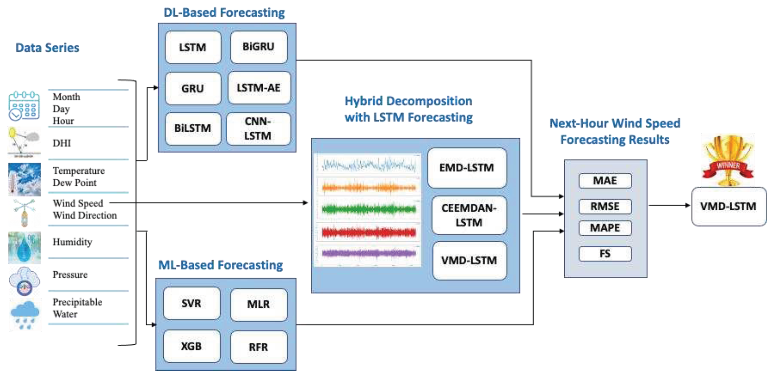
Figure 1. Graphical abstract.
Preprints 86091 g001
Figure 2. Wind dataset locations on Saudi Arabia map.
Preprints 86091 g002
Figure 3. Toronto and Caracas locations on a map.
Preprints 86091 g003
Figure 4. Correlation matrix (Alghat).
Preprints 86091 g004
Figure 5. Correlation matrix (Dumat Aljandal).
Preprints 86091 g005
Figure 6. Correlation matrix (Waad Alshamal).
Preprints 86091 g006
Figure 7. Correlation matrix (Yanbu).
Preprints 86091 g007
Figure 8. Correlation matrix (Caracas).
Preprints 86091 g008
Figure 9. Correlation matrix (Toronto).
Preprints 86091 g009
Figure 10. a) ACF of WS (Alghat); (b) ACF of WS (Dumat Aljandal); (c) ACF of WS (Waad Alshamal); (d) ACF of WS (Yanbu); (e) ACF of WS (Caracas); (f) ACF of WS (Toronto).
Preprints 86091 g010Preprints 86091 g011
Figure 11. Correlation matrix of feature set (Alghat).
Preprints 86091 g012
Figure 12. Correlation matrix of feature set (Dumat Aljandal).
Preprints 86091 g013
Figure 13. Correlation matrix of feature set (Waad Alshamal).
Preprints 86091 g014
Figure 14. Correlation matrix of feature set (Yanbu).
Preprints 86091 g015
Figure 15. Correlation matrix of feature set (Caracas).
Preprints 86091 g016
Figure 16. Correlation matrix of feature set (Toronto).
Preprints 86091 g017
Figure 17. EMD results of (a) Alghat; (b) Dumat Aljandal; (c) Waad Alshamal; (d) Yanbu; (e) Caracas; (f) Toronto.
Preprints 86091 g018Preprints 86091 g019
Figure 18. CEEMDAN results of (a) Alghat; (b) Dumat Aljandal; (c) Waad Alshamal; (d) Yanbu; (e) Caracas; (f) Toronto.
Preprints 86091 g020Preprints 86091 g021
Figure 19. VMD results of (a) Alghat; (b) Dumat Aljandal; (c) Waad Alshamal; (d) Yanbu; (e) Caracas; (f) Toronto.
Preprints 86091 g022
Figure 20. LSTM model.
Preprints 86091 g023
Figure 21. GRU model.
Preprints 86091 g024
Figure 22. BiLSTM model.
Preprints 86091 g025
Figure 23. BiGRU model.
Preprints 86091 g026
Figure 24. CNN-LSTM model.
Preprints 86091 g027
Figure 25. LSTM-AE model.
Preprints 86091 g028
Figure 26. LSTM combined with decomposition methods.
Preprints 86091 g029
Figure 27. Hybrid model of decomposition methods and LSTM.
Preprints 86091 g030
Figure 28. MAE results (weather features).
Preprints 86091 g031
Figure 29. MAE results (WS lagged features).
Preprints 86091 g032
Figure 30. RMSE results (weather features).
Preprints 86091 g033
Figure 31. RMSE results (WS lagged features).
Preprints 86091 g034
Figure 32. MAPE results (weather features).
Preprints 86091 g035
Figure 33. MAPE results (WS lagged features).
Preprints 86091 g036
Figure 34. WS hourly average per month.
Preprints 86091 g037
Figure 35. Forecasting results per month: (a) MAE; (b) RMSE; and (c) MAPE for Alghat; (d) MAE; (e) RMSE; and (f) MAPE for Dumat Aljandal; (g) MAE; (h) RMSE; an (i) MAPE for Waad Alshamal (j); MAE; (k) RMSE; and (l) MAPE for Yanbu; (m) MAE; (n) RMSE; and (o) MAPE for Caracas; (p) MAE; (q) RMSE; and (r) MAPE for Toronto.
Preprints 86091 g038Preprints 86091 g039
Figure 36. MAE results of 13 models.
Preprints 86091 g040
Figure 37. RMSE results of 13 models.
Preprints 86091 g041
Figure 38. MAPE results of 13 models.
Preprints 86091 g042
Figure 39. Comparing the effect of using decomposition methods to the effect of using weather variables: (a) MAE results; (b) RMSE results; and (c) MAPE results.
Preprints 86091 g043
Figure 40. Forecast skill of all models (MAE).
Preprints 86091 g044
Figure 41. Forecast skill of all models (RMSE).
Preprints 86091 g045
Figure 42. Forecast skill of all models (MAPE).
Preprints 86091 g046
Table 1. Summary of the related work.
Ref No. Objective Method Features Data source Results
[15] WS CNN-BiLSTM WS, Maximum WS, SD of WS Ground-based MAE=0.30, RMSE=0.43, MAPE=115 for a location in SA
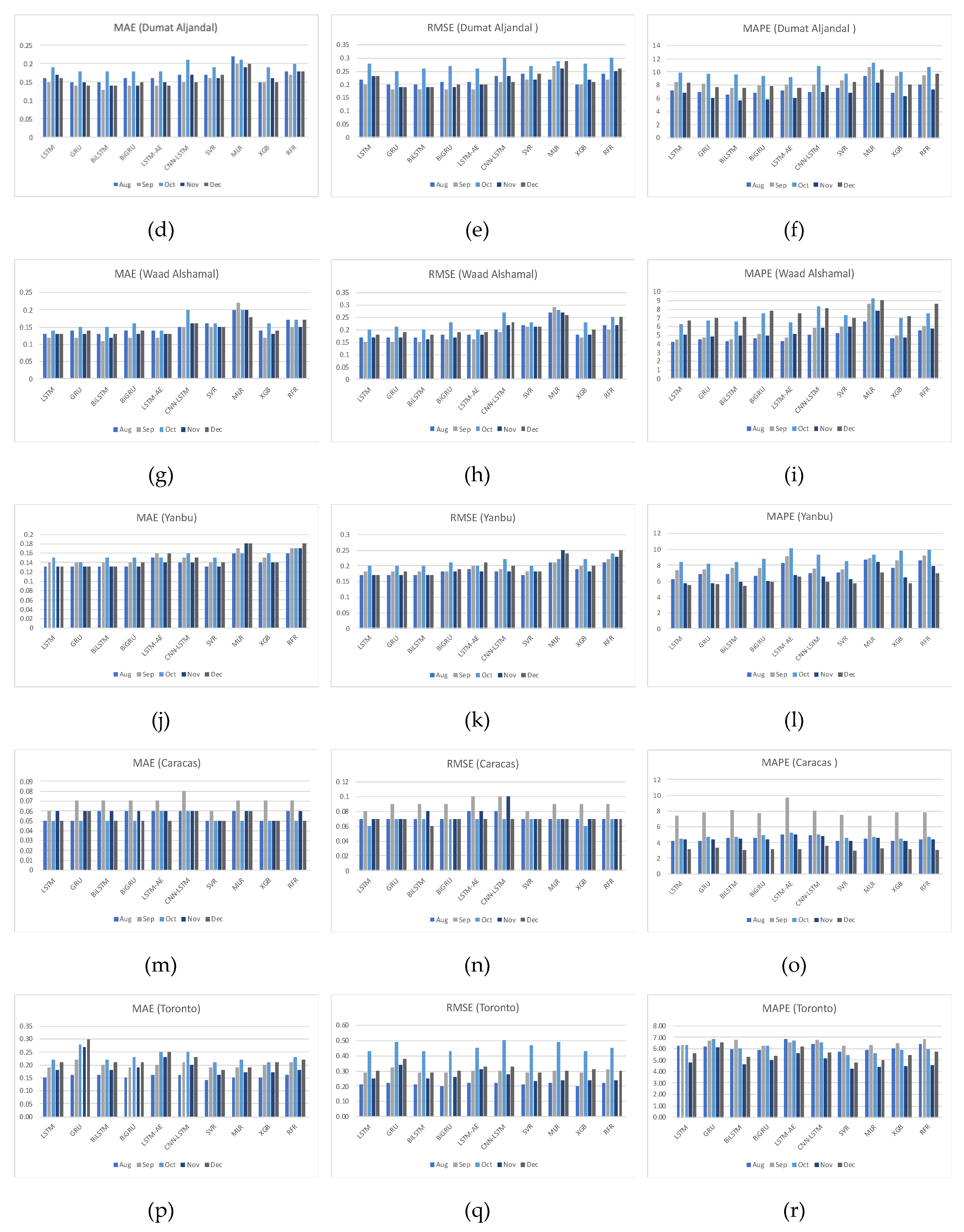
[16] WS SVR WS Ground-based MAE=2.37, MAPE= 206.80 for Yanbu, SA
[17] WS RR WS, WD, PWS, T, P, RH Mesoscale atmospheric model MAE=1.22, RMSE=0.26, R2=0.9 for a city in SA
[18] WS LSTM WS, T, P Ground-based MAE=0.28, R2=0.97 for Dhahran, SA
[19] WS ESN WS Simulated data by WRF MSE= 0.24 for a location in SA
[20] WS BiLSTM WS, GHI, DNI, DHI, T Simulated data MAE=0.4, RMSE=0.6, MAPE=15, R2=0.93 for Dumat Aljandal, SA
[21] WS GRU WS, T Simulated data MAE=0.48, RMSE=0.66, MAPE=5, R2=0.93 for Dumat Aljandal, SA
[22] WS FFNN T, WD, GHI, PWS, RH, P Ground-based RMSE =0.81, R=0.92, MAE=0.61 for Jeddah, SA
RMSE =0.54, R=0.87 for Riyadh, SA
RMSE =0.86, R=0.90, for Taif, SA
RMSE =1.12, R=0.90, for Afif, SA
[23] WS FFNN WS, T, RH Ground-based MAPE =6.65%, MSE = 0.09 for Qaisumah village, SA
[12] WS MLP, CNN, RNN WS Simulated data by WRF R2 for CNN and RNN model is higher than MLP in USA
[14] WS CNN T, RH, P, WS, season, month, day, hour Simulated data by PSM MAE=0.09, RMSE=0.23, sMAPE=4.92 for USA
[13] WS Hybrid model of WSTD+ GRU WS Ground-based MAE=0.23, RMSE=0.38, MAPE=0.01 for Bondvill, USA
MAE=0.17, RMSE=0.26, MAPE=0.07 for Penn State University, USA
MAE=0.40, RMSE=0.53, MAPE=0.03 for Boulder, USA
MAE=1.26, RMSE=1.86, MAPE=0.19 for Desert Rock, USA
[24] WS Hybrid model of CEEMDAN+ PE+ GRU+RBFNN +IBA WS Ground-based MAE=0.45, RMSE=0.59, MAPE=4.79% for Zhangjiakou, China
[25] WS Hybrid model of EMD+VMD+ XGB+ CGRU+ GA WS Ground-based RMSE=0.57, MAE=0.41, MAPE=8.36%
for Shandong Province of China
[26] WS Hybrid model of VMD+LN+ MOBBSA+ LSTM-AE WS Ground-based MAE= 0.08, RMSE=0.11, MAPE=2.95%
for Rocky Mountains, USA
[27] WP Hybrid model of VMD+ residual-based CNN WP, WS, WD Ground-based R= 0.97, RMSE=0.05, MAE=0.04 for a location in Turkey
[28] WP & WS Hybrid model of VMD+ SIRAE WP, WS Ground-based RMSE= 1.23% for Galicia, Spain
MAE= 2.45%, RMSE=3.16% for Dodge City, USA
[29] WS Hybrid model of VMD+ ESN+DE WS, WD, T, P, RH, Ground-based RMSE= 0.12, MAE= 0.10, MAPE= 2.6% for Galicia, Spain
*T: Temperature, P: Pressure, WD: Wind Direction, RH: Relative Humidity, PWS: Peak Wind Speed, SD: Standard Deviation, GHI: Global Horizontal Irradiation, DNI: Direct Normal Irradiance, DHI: Diffuse Horizontal Irradiance.
Table 2. Saudi dataset location information.
Location No. Location Name Latitude (N) Longitude (E) Elevation (m)
1 Alghat 26.32 43.45 674
2 Dumat Aljandal 29.52 39.58 618
3 Waad Alshamal 31.37 38.46 747
4 Yanbu 23.59 38.13 10
Table 3. International dataset location information.
Location Name Latitude (N) Longitude (E) Elevation (m)
Caracas, Venezuela 10.49 -66.9 942
Toronto, Canada 43.65 -79.38 93
Table 4. Saudi dataset features.
Time t features Time t1 features WS lagged features
WS (output) T_lag1 WS_lag1
DHI_lag1 WS_lag2
HS DP_lag1 WS_lag3
HC RH_ lag1 WS_lag4
DS P_lag1 WS_lag5
DC PW_lag1 WS_1D
WDS_lag1
WDC_lag1
Table 5. Caracas and Toronto dataset features.
Common features Caracas only Toronto only
WS (output) T_lag1 WS_lag1 WS_1D WS_lag8
DP_lag1 WS_lag2 DNI_lag1 WS_lag9
HS RH_ lag1 WS_lag3 WS_lag10
HC P_lag1 WS_lag4 WS_lag11
DS PW_lag1 WS_lag5 WS_lag12
DC WDS_lag1 WS_lag6 GHI_lag1
WDC_lag1 WS_lag7
Table 6. Dataset descriptions.
Dataset WS mean WS SD WS VAR WS MIN WS MAX
Alghat Train: 3.03 1.53 2.33 0.1 10
Val: 3.13 1.58 2.50 0.2 8.6
Test: 3.01 1.43 2.04 0.2 9.2
All: 3.04 1.52 2.31 0.1 10
Dumat Aljandal Train: 2.65 1.40 1.97 0.1 9.8
Val: 2.79 1.55 2.39 0.1 10.3
Test: 2.62 1.37 1.87 0.1 7.3
All: 2.66 1.42 2.02 0.1 10.3
Waad Alshamal Train: 3.08 1.56 2.44 0.2 10.6
Val: 3.40 1.69 2.86 0.4 11.1
Test: 2.97 1.39 1.93 0.2 9.3
All: 3.12 1.56 2.44 0.2 11.1
Yanbu Train: 3.17 1.61 2.58 0.1 11.2
Val: 3.31 1.70 2.89 0.1 9.9
Test: 3.06 1.58 2.50 0.2 9.6
All: 3.17 1.62 2.62 0.1 11.2
Caracas Train: 1.63 0.42 0.17 0.1 2.9
Val: 1.76 0.34 0.12 0.8 2.7
Test: 1.39 0.39 0.15 0.1 2.6
All: 1.62 0.42 0.17 0.1 2.9
Toronto Train: 4.38 2.37 5.60 0.1 14.7
Val: 3.85 2.49 6.17 0.3 15.6
Test: 4.28 2.07 4.29 0.3 14.1
All: 4.28 2.35 5.52 0.1 15.6
Table 7. DL-based Models’ hyperparameters and optimization methods.
Hyperparameter Value Optimization
Learning Rate 0.001 Adam Optimizer
Number of Epochs 100 Activation Function= ReLU, Tanh*
Dropout 0.1 Loss Function= MSE
Batch Size 500 Early Stopping
Weight Decay 0.000001 Kernel Initializer= glorot uniform
* In hybrid LSTM model with decomposition methods.
Table 8. Features used to train the models.
Time t features Time t-1 features WS features
WS (output) T_lag1 WS_lag1
DHI_lag1 WS_lag2
HS DP_lag1 WS_lag3
HC RH_ lag1 WS_lag4
DS P_lag1 WS_lag5
DC PW_lag1 WS_1D
WDS_lag1
WDC_lag1
Disclaimer/Publisher’s Note: The statements, opinions and data contained in all publications are solely those of the individual author(s) and contributor(s) and not of MDPI and/or the editor(s). MDPI and/or the editor(s) disclaim responsibility for any injury to people or property resulting from any ideas, methods, instructions or products referred to in the content.
Copyright: This open access article is published under a Creative Commons CC BY 4.0 license, which permit the free download, distribution, and reuse, provided that the author and preprint are cited in any reuse.
Prerpints.org logo

Preprints.org is a free preprint server supported by MDPI in Basel, Switzerland.

Subscribe

© 2024 MDPI (Basel, Switzerland) unless otherwise stated