
Submitted:
25 September 2023
Posted:
27 September 2023
You are already at the latest version
Abstract
Techniques and tools meant to aid fire management activities in the Cerrado, such as accurately determining fuel load and composition spatially and temporally, are pretty scarce. The need to have fuel information for more efficient management in a considerably heterogeneous, biodiverse, and fire-dependent environment makes a constant search for the improvement of the use of remote sensing techniques in determining fuel characteristics. This study presents the following objectives: (1) to assess the use of data from Landsat 8 OLI images to estimate the fine surface fuel load of the Cerrado during the dry season by adjusting multiple linear regression equations; (2) to estimate fuel load through Random Forest and k-Nearest Neighbor (k-NN) algorithms in comparison with re-gression analyses; and (3) to evaluate the importance of predictor variables from satellite images. Therefore, 64 sampling units were collected, and the pixel values associated with the field plots were extracted in a 3 x 3 pixel window surrounding the reference pixel. For the multiple linear regression analyses, the R² values ranged from 0.63 to 0.78, and the models fitted by the Random Forest al-gorithm ranged from 0.52 to 0.83, while those fitted by k-NN ranged from 0.30 to 0.68. Adopting the Random Forest algorithm resulted in improvements in the statistical metrics of evaluation of the fuel load estimates for Cerrado grassland relative to the multiple linear regression analyses.
Keywords:
fuel load
; satellite imagery
; image processing
; fuel load maps
; fuel estimation
1. Introduction
Fire is common in the Cerrado biome, mainly in open plant physiognomies predominated by herbaceous and grassland vegetation. According to Miranda et al. [1], fires in the Cerrado, like in other savannas, can be characterized as surface fires that consume the fine fuels of the grass fuel layer. Surface fine fuels represent the layer of particles less than 0.6 cm in thickness, consisting of litter, grasses, herbs, and downed woody material [2]. For Rothermel [3], the fuel represents the organic matter available for ignition and combustion and characterizes the only fire-related factor that can be controlled by human action. Knowing the fuel characteristics is essential to determining fire behavior and decision-making in integrated fire management and wildfire suppression actions. However, determining the characteristics of the fuel is temporally and spatially complex [4,5]. Arroyo et al. [6] reported that determining fuel characteristics demands high costs and considerable time for sampling. Roberts et al. [7] indicate the following essential attributes in understanding fire behavior: fuel type, fuel biomass, fuel moisture, and fuel condition (live or dead). Fuel load is a crucial variable, commonly used fuel characteristic in various fire management strategies, such as fire risk assessments and fire behavior prediction [3]. Nevertheless, there are few studies on the Cerrado that involve determining the characteristics of its flammable material.
Remote sensing techniques are essential for estimating several fuel characteristics as more studies and improvements are made. According to Roberts et al. [7], the products obtained from various remote sensing techniques can help assess wildfire hazards, which include the following: (i) direct measurements of live fuel moisture, (ii) measurements of live herbaceous biomass, (iii) measurements of fuel condition, (iv) detailed classifications of fuel type. Van Wagtendonk and Root [8] note that information relative to fuel is often presented as fuel model maps; fuel models are used to determine fuel load, size, depth, and moisture of extinction. A wide range of studies have estimated fuel variables through remote sensing products. However, there is a significant lack of studies concerning the surface fuel of grassland environments of the Cerrado biome. Several studies characterize and estimate forest biomass using Landsat imagery [9,10,11,12], MODIS products [13,14], and Lidar sensors [15,16]. Various studies that use remote sensing products mostly relate to the characterization of forest variables, but few works with estimates of surface fuel variables, which are more related to the occurrence of surface fires, quite recurrent in grassland and savanna areas.
The use of vegetation indices has been widely addressed. They are utilized in biomass studies and mainly to determine the fuel moisture [17,18]. Other studies using spectral mixture techniques have been conducted [19,20]. However, few are related to determining surface fuel's physical characteristics, except for Franke et al. [21], who applied spectral mixture techniques to map fine fuel accumulation. In this sense, the main objectives of the present study are as follows:
- (1)
- To evaluate the performance of multiple linear regression equations adjusted for load estimation in classes of live and dead fine fuels, considering the beginning and end of the dry season, based on the reflectance of Landsat 8 OLI images, vegetation indices, and fraction values (F-values) of the spectral mixture analysis (SMA);
- (2)
- To assess the use of Random Forest and k-Nearest Neighbor algorithms to estimate fine fuel load in different classes in comparison to traditional multiple linear regression analyses;
- (3)
- To analyze the importance of each predictor variable from remote sensing products in Random Forest models.
2. Materials and Methods
2.1. Study Area
Collections in the field were made in the central southern portion of the Serra Geral do Tocantins Ecological Station (EESGT), a fully protected conservation unit with an area of 716,306 ha located in the Cerrado biome in the Jalapão region. According to the Köppen climate classification, the region’s climate is classified as Aw (tropical savanna climate), and its annual precipitation ranges from 1,400 to 1,500 mm [22], which is higher than the annual potential evapotranspiration. In the region, the summer occurs between October and April and is rainy, and winter occurs between May and September and is dry [23]. The predominant plant physiognomy is grassland: pure grassland (campo limpo), pure wet grassland (campo limpo úmido), grassland with scattered shrubs and trees (campo sujo), wet grassland with scattered shrubs and trees (campo sujo úmido), and rocky grassland (campo rupestre) [24,25]. The predominant type of soil type is quartz sand or quartzipsamments, and it has a sandy or loamy texture at least two meters deep and may have up to 15% clay. The location’s relief varies from relatively flat to gently undulating, with average elevations between 300 and 500 meters [26]. Figure 1 presents the study area and the spatial distribution of sampling data units.
2.2. Field Survey
A field survey of the variables of surface fuel load was conducted by installing data sampling units that were collected during the period from 05/11/2017 to 05/31/2017 (May), from 06/06/2017 to 06/29/2017 (June), from 08/05/2017 to 08/25/2017 (August) and; from 09/08/2017 to 09/24/2017 (September). Average air temperatures at the time of samplings ranged from 24.4 to 31.0 °C from the beginning (May and June) to the end (August and September) of the dry season, respectively. The relative humidity of the air presented averages at the time of samplings, which varied from 41.0 to 27.3% from the beginning to the end of the dry season. Each sampling unit had two 30-meter transects spaced 14 meters apart. Markings were made on the transects to install by prior draw eight sub-samples of surface fuel with an area of 0.25 m² (0.5 x 0.5 cm), and fuel was collected from them by the destructive method. The size of the sub-samples was chosen for a broader sampling that could provide a more significant variability of fuel samples in a shorter time. Accordingly, 64 data sampling units separated by a distance over 100 m from each other were collected for analyses by satellite images. It is noteworthy that data sampling was carried out in the area of viable access, given the existence of an area of difficult access further north (Figure 1).
The destructive sampling involved separating the material according to its physiological state (live or dead) among different diameter classes (timelag), adapting the methodology proposed by Schroeder and Buck [27] and Brown et al. [2]. Thus, the surface fuels were classified as follows: (i) dead grass fuel, (ii) 1-h downed wood debris (<0.64 cm diameter), (iii) live grass fuel, and (iv) live shrub fuel (<0.64 cm diameter). As the study aims to estimate fine fuels under 0.64 cm in diameter, which exert more significant influence on fire spread in regions with open vegetation in the Cerrado biome, the 10-h (0.64 - 2.54 cm) and 100-h (2.54 - 7.62 cm) classes are not considered. In addition to the abovementioned classes, the analyses and estimates took into account the total fine live (grass + shrub <0.64 cm diameter) and fine dead (grass + 1-h downed wood debris) fuels and the total fine fuel load (live and dead; <0.64 cm diameter). After collecting the sub-samples from the field, they were all dried until they reached constant mass. Next, the dry mass was determined, and its respective fuel moisture content was calculated by the ratio between wet mass and dry mass on a dry weight basis and then converted to percentage. Figure 2 presents a diagram exemplifying the collection locations, surface fuel data sampling, and characterization process.
2.3. Obtaining and Processing Satellite Imagery
Images from the Landsat 8 OLI satellite were used in this study. They were obtained for the approximate dates of four collections of field samples during the dry season in May and June (beginning of the dry season) and in August and September (end of the dry season), corresponding to the following dates (mm/dd/yyyy): 05/05/2017, 06/06/2017, 06/22/2017, 07/24/2017, 08/09/2017, and 09/10/2017. To cover the entire study area, images from 3 Landsat 8 OLI scenes were used, namely: 220/067; 221/067, and; 221/068. The reflectance values of the bands were extracted, and the vegetation indices were calculated through the cloud-based geospatial data processing platform Google Earth Engine (GEE). The GEE platform provides easy access to high-performance computing resources for large-scale processing of geospatial datasets [28]. The reflectance values were obtained from the Landsat 8 OLI sensor bands in the following channels: (i) blue (0.45 - 0.51 µm), (ii) green (0.53 - 0.59 µm), (iii) red (0.64 - 0.67 µm), (iv) near-infrared (0.85 - 0.88 µm), (v) short-wave infrared (1.57 - 1.65 µm), and (vi) short-wave infrared (2.11 - 2.29 µm).
2.3.1. Vegetation Indices (VIs)
Based on the combination of reflectance in different spectral bands, vegetation indices (VIs) were calculated. VIs are an efficient way to attain empirical information from multispectral sensors and are frequently used in various scientific studies that set out to explain better or determine the behavior of certain vegetation variables [8,9,29,30]. Therefore, a total of 20 vegetation indices were calculated and incorporated into the analyses as independent variables: (i) Normalized Difference Vegetation Index - NDVI [31]; (ii) Visible Atmospherically Resistant Index - VARI [32]; (iii) Visible Green Index - VIgreen [32]; (iv) Simple Ratio - SR [33]; (v) Structure Insensitive Pigment Index - SIPI [34]; (vi) Soil-adjusted Vegetation Index - SAVI [35]; (vii) Normalized Difference Water Index - NDWI [36]; (viii) Normalized Difference Infrared Index - NDII6 [37]; (ix) Normalized Burn Ratio - NBR [37]; (x) Modified Vegetation Index - MVI [38]; (xi) Modified Simple Ratio - MSR [39]; (xii) Moisture Stress Index - MSI [40]; (xiii) Modified Normalized Difference Water Index - MNDWI [41]; (xiv) Integral - INT [42]; (xv) Global Vegetation Moisture Index - GVMI [29]; (xvi) Enhanced Vegetation Index - EVI [43]; (xvii) Derivative - band 5 (ivp), band 6 (siwir1) - DER56 [44]; (xviii) Derivative - band 4 (vm), band 5 (ivp) - DER45 [44]; (xiv) Derivative - band 3 (vd), band 4 (vm) - DER34 [44]; (xx) Derivative - band 2 (az), band 3 (vd) - DER23 [44]. The vegetation indices analyzed in this study show relationships with fuel load and moisture, as well as with the physiological state of the fuel. The choice of these vegetation indices aimed to analyze their viability for estimating fuel load from Landsat 8 OLI images, considering seasonality during the dry season in a Cerrado environment.
2.3.2. Spectral Mixture Analysis (SMA)
The spatial variability of vegetation within a pixel is a strong limiting factor in ascertaining fuel condition and load information. Spectral Mixture Analysis (SMA) has considerable potential to estimate fuel condition and fuel moisture content at the sub-pixel level [30]. SMA is a widely applied technique in remote sensing for obtaining ecologically relevant and significant components of an image pixel [45]. In SMA, two or more reference spectra (endmembers), such as green vegetation, dry vegetation, soil, and shade, are modeled as linear combinations to estimate the sub-pixel fractions of each component [46].
After retrieving the Landsat 8 OLI images, they underwent the atmospheric correction process to eliminate interferences from the atmosphere to extract data and determine the reflectance values [47]. Next, the color composites were obtained and utilized in subsequent study steps. The color composite of the Landsat 8 OLI image used in the initial collection for the spectral mixture analyses was 7 (short-wave infrared - SWIR 2), 5 (near-infrared), and 4 (red). After processing the satellite images, the creation of a spectral library began. First, the surface targets for the SMA were divided into (i) non-photosynthetic dry vegetation (NPV), (ii) green vegetation (GV), and (iii) exposed soil. This classification was chosen because green vegetation, dry vegetation, and soil dominate Cerrado grassland environments. Figure 7 presents the fuel condition mapping demonstrating the accumulation of GV, NPV fuel, and soil from the EESGT contrasting the early and late dry season condition fuel in the Cerrado biome. Several candidates for “pure pixels,” known as endmembers, were selected from each target. Thus, based on the specific spectral behavior of each target, regions of interest (ROI) whose reflectance presented spectral behaviors that were as faithful as possible to the characteristic spectral curve of the respective target were delimited.
To fulfill the objectives proposed herein, endmembers were chosen in four representative images of the four months of the dry season (May, June, August, and September), according to the dates of the Landsat 8 images previously mentioned. Having chosen all the pure pixel candidates of the features as mentioned earlier based on the spectral curves, the process of selecting the endmembers based on the lowest statistical errors began. The multiple endmember spectral mixture analysis (MESMA) methodology was applied to perform this procedure. MESMA’s results produce gray-scale images whose values (called fraction values – F-values) represent the estimated relative degree in which each pixel corresponds to its respective reference spectrum. Therefore, the images generated with the F-values were for the GV, NPV, and soil components.
2.3.3. Data Extraction
The pixel values associated with the field plots were extracted from a 3 x 3-pixel window around the reference pixel (pixel associated with the field plot). This way, the median values of the pixels in each 3 x 3-pixel polygon related to the field plots were extracted [9,10,48,49,50,51,52]. The data were exported and tabulated to compare the information collected from the plots in the field with the information from the spectral mixture analysis, reflectance, and the calculated vegetation indices.
2.4. Statistical Analysis of the Data
2.4.1. Multiple Linear Regression Analysis
After processing the data from the Landsat 8 OLI satellite images, all the information associated with the collection points in the field were extracted in a 3 x 3-pixel window. Then, all the data were tabulated and correlated with the fuel load values in the different classes. In the multiple linear regression analyses, fuel load was a dependent variable, especially for the fine dead fuels (dead grass fuel, 1-h downed wood debris, and total fine dead fuel) and total fine fuel (live and dead, <0.64 cm diameter) classes. The predictor (independent) variables were divided into three main groups: (i) fraction values (F-values) from the spectral mixture analyses (SMA), (ii) the reflectance of the Landsat 8 OLI images in the different spectral bands, and (iii) the calculated vegetation indices. The stepwise method was adopted to select the most relevant variables for the regression equations. Also, the adjustments of the multiple linear regression equations considered the following: (i) adjusting equations considering 32 plots collected in the initial months of the dry season (May and June), (ii) adjusting equations considering 32 plots collected in the final months of the dry season (August and September), and (iii) adjusting equations for the entire period of the dry season (all 64 plots). Figure 3 presents a flowchart of the methodology applied in this study.
2.4.2. Random Forest Machine Learning Algorithm
The Random Forest (RF) machine learning algorithm is a non-parametric method developed by Breiman [53] that has been widely adopted in various studies [11,14,51,54]. The RF algorithm combines several predictor trees generated by an independently sampled random vector with a similar distribution for all trees in the forest [55]. Compared to traditional linear regression methods, Random Forest models exhibit several advantages in aboveground biomass estimation, such as better accuracy and fewer non-linear problems [56].
Although the training and test sets were divided randomly in R, a specific code command (set seed) was used to guarantee the model’s reproducibility, in other words, to run the model with the same previously defined data sets (training and test). To implement Random Forest, two parameters must be defined: the number of trees (ntree) and the number of features in each split (mtry). Regarding the ntree, in the present study, it was observed that the prediction accuracy by the Random Forest algorithm did not increase significantly when the ntree presented values greater than 1,000. The ideal ntree defined was ntree = 1,000 to guarantee the reliability of the prediction results without affecting computational efficiency [57,58]. For mtry, the values were defined as one-third of the total number of predictor variables [53,59,60,61]. These varied between mtry = 4 and 5 for models adjusted with predictor variables selected by the stepwise method and mtry = 10 for models adjusted with all predictor variables. The “randomForest” package in R program was used to apply the algorithm. The importance of the predictor variables utilized in the Random Forest models was evaluated by the increase in the mean squared error (% IncMSE), which measures the effect of a variable’s predictive potential when subjected to a random permutation. In short, this metric shows how much the model’s accuracy decreases if a particular predictor variable is left out of the model.
2.4.3. K-Nearest Neighbor Machine Learning Algorithm
Another machine learning algorithm used to verify the feasibility of estimating fuel load from satellite imagery products was the k-Nearest Neighbor (k-NN) algorithm. The k-NN algorithm is used for classification and regression. It predicts the values of specific variables based on the similarity in a covariate space between the point and other points representing the values of the variables [62]. The utilization of the k-NN algorithm associated with remote sensing data has played a key role in forest studies, and there have been several applications in forest inventories in the field that aimed to improve the accuracy of estimates [63,64]. The k-NN algorithm was applied employing the “Caret” package in R. There is one essential parameter in this algorithm, K, or the number of neighbors that need to be optimized. This parameter specifies the voting system in the k-NN algorithm wherein the K nearest neighbors are selected, and then it sets the output model [65]. The K values were determined based on the lowest RMSE values, and the optimal values were chosen for each estimated fuel variable. Table 3 provides each estimated fuel variable's selected K values and the respective RMSE values.
2.4.4. Cross-validation
Cross-validation evaluates a model’s performance and provides a nearly unbiased prediction error estimator [66]. The multiple linear regression equations, Random Forest models, and k-NN algorithm models were subjected to cross-validation with the k-fold cross-validation technique, using 10 folds. The k-fold cross-validation technique is a robust method for estimating a model’s accuracy, and it generally provides more accurate estimates of the test error rate [9,67,68]. The following statistical metrics were used to validate the equations: (i) the values of the squared coefficient of determination (R²), (ii) the adjusted squared coefficient of determination (R²adj), (iii) the root-mean-square error (RMSE), and (iv) the mean absolute error (MAE). The validations considered the adjustments of the multiple linear regression models and the Random Forest and k-Nearest Neighbor algorithm models, with an emphasis on the models with the best fit considering all the independent variables of the study and on the models with the best fit considering the independent variables selected by the stepwise method.
3. Results
3.1. Multiple Linear Regression Analysis
Table 1 presents the metrics of the multiple linear regression equations, which were validated by considering the study's independent variables. The multiple linear regression equations performed best with the adjustments by the stepwise method. Table 1 presents only the metrics of the equations adjusted by this method. The equations validated by the k-fold cross-validation method, which were notable about the coefficient of determination (R²), were for the estimation of total fine dead fuel (grass + 1-h downed wood debris), with R² = 0.92, and dead grass fuel, with R² = 0.89. These equations mentioned earlier are for the beginning of the dry season (p < 0.05). However, the lowest RMSE and MAE values were observed for estimates of dead grass fuel at the beginning of the dry season, with values below 0.40. The statistical metrics verified for the end of the dry season were lower than those observed for the equations adjusted for the beginning of the dry season in the study area.
For the entire period of the dry season, the R² values ranged from 0.57 to 0.78. The equation for estimating dead grass fuel performed the best, with R² = 0.78, followed by the stepwise equation for calculating total fine dead fuel (grass + 1-h downed wood debris), with R² = 0.73 (p < 0.05). The R²aj values of the equations subjected to cross-validation may be negative without a lower limit and present a maximum value of one, as noted by Peterson et al. [69], which was the case for the equations at the end of the dry season. The lowest RMSE and MAE values were found to estimate dead grass fuel.
3.2. Estimates by the Random Forest Algorithm
3.2.1. Model Performance Metrics
To use the Random Forest algorithm, the entire dry season was considered for the adjustment of the models. The models were not divided for the dry season's beginning and end, as was done for the multiple linear regression analyses. Like the regression equations, the Random Forest algorithm was adjusted for each estimated variable by considering all the study's independent variables and the variables selected by the stepwise method. Unlike the multiple linear regression equations, the Random Forest models presented a slight advantage in the adjustments with all the independent variables compared to the adjustments with the variables selected by the stepwise method, as shown in Table 2. The R² values by the Random Forest algorithm ranged from 0.52 to 0.83; the highest values were found to estimate dead grass fuel and total fine dead fuel.
To estimate the total fine fuel (live and dead), the best performance was related to the model using all the independent variables, with R² = 0.62. As for the RMSE and MAE values of the estimates by the Random Forest algorithm, the lowest values were recorded for the estimation of dead grass fuel, with 0.33 and 0.23, respectively. In contrast, the highest RMSE and MAE values corresponded to the estimation of total fine fuel load (live and dead). Figure 4 and Figure 5 show the fine fuel load mappings in the Serra Geral do Tocantins Ecological Station, with the best fits for each fuel load category analyzed.
3.2.2. Importance of the Variables in the Random Forest Models
In analyzing the results of the importance of the variables in the RF models presented in Figure 6, the considerable importance of the fraction-soil variable (FS – F-values) from the spectral mixture analysis (SMA) is noteworthy in all the models addressed. In all situations, the FS variable increased the mean squared error (% IncMSE) above 20% in all the models presented. This means that the removal of the predictor variable FS will result in an increase in the mean squared error above 20% for the estimated fuel variables. Among the fuel variables in which FS exerted greater importance, total fine dead fuel (grass + 1-h downed wood debris) and dead grass fuel were notable, presenting values of 33.5% and 29.1%, respectively.
The vegetation indices NDII, NBR, GVMI, and DER56 emerged as the second most essential variables considering the estimates of dead grass fuel, 1-h downed wood debris, total fine dead fuel (grass + 1-h downed wood debris), and total fine fuel (live and dead), respectively. GVMI appeared most frequently among the vegetation indices and was most important in the fitted Random Forest models. It was not a variable of importance only for estimating total fine fuel. Out of the bands' reflectance, the short-wave infrared channel (SWIR2 - 2.11 - 2.29 µm) occurred most frequently and had the most significant importance. Figure 6 graphically illustrates the importance of the Random Forest algorithm models with the best fit.
3.3. Estimates by the K-Nearest Neighbor Algorithm
Similarly, the data from the same database used for the application of the RF algorithm were executed with the k-Nearest Neighbor (k-NN) algorithm so that two models were built for each fuel load variable: one model considering all the independent variables of the study and another model considering only the variables selected by the stepwise method. As a parameter for using the k-NN algorithm, the K values were chosen based on the lowest RMSE values, ranging from 5 to 13. Table 3 demonstrates the K values chosen for each k-Nearest Neighbor algorithm model.
Like the Random Forest models, the k-Nearest Neighbor models presented slightly superior performances for the adjustments made with all the predictor variables of the study in comparison with those selected by the stepwise method. The R² values ranged from 0.30 to 0.68, and the k-NN models with the best fit were for estimating dead grass fuel, followed by the model for estimating total fine dead fuel, with R² = 0.54. Table 4 provides the statistical metrics of the k-NN algorithm models.
Regarding the RMSE and MAE values, the estimates by the k-NN algorithm presented the lowest values for the estimation of dead grass fuel, with 0.37 and 0.30, respectively. The highest RMSE and MAE values about the k-NN models were found to estimate total fine fuel load (live and dead) (Table 4).
4. Discussion
Given the low correlations of the live fuel classes (live grass and live shrub), the statistical analyses for their estimation could not be conducted. However, according to the findings of Santos et al. [70], the low moisture level for Cerrado grassland species is the main factor behind the increase in the fuel’s flammability. Moreover, the proportion of fine dead fuel about the proportion of live fuel during the dry season in the biome can reach 70%, or over 80%, considering only the grass fuel of the area, based on the fuel characterization by Santos et al. [71]. In addition, the fine thickness of 1-h and grass fuels in a physiologically inactive state (e.g., grass and 1-h downed wood debris) makes the moisture content of these fuels more sensitive to changes in atmospheric conditions, thus affecting their ignition capacity and leaving areas with a predominance of these types of fuels more prone to the occurrence of wildfires, especially in the dry season [72]. As reported by Slijepcevic et al. [73] and Soares et al. [74], low fuel moisture is one of the main factors contributing to the occurrence of large fires.
Out of the adjustments of the multiple linear regression equations for the beginning and end of the dry season in the Cerrado biome, the equations adjusted for the beginning of the dry season had the best statistical performance. This may be explained by analyzing the results obtained by Santos et al. [71], who characterized the fuel of Cerrado grassland vegetation. In this study, fuel characteristics, such as the number of individuals, the number of species, the grass height, and the fuel load in different classes (timelag), exhibit different behaviors between the first and last months of the dry season in the physiognomy under analysis. The fuel condition mapping showing fractions of NPV, GV, and soil for the beginning of the dry season (May) in contrast to the fuel condition at the end of the dry season (September) is presented in Figure 7. For example, given the different ages of the fuels present in the area, the load values of dead grass fuel in the first months of the dry season (May and June) showed a statistically significant difference in dead grass fuel between the ages of one and four years. By the end of the dry season (August and September), no statistically significant difference was found among the fuel loads of dead grass fuels between the ages of two and four years (p < 0.05).
Considering all the adjustments of the multiple linear regression equations in the study (beginning, end, and the entire dry period), the R² values ranged from 0.45 to 0.92. For the whole of the dry period, the highest value was 0.78 for the adjusted equation to estimate dead grass fuel (Table 1). Similar results were reported by Tucker et al. [75], who presented more expressive values considering only coefficient of determination (R²) values and the 0.385 µm range of the electromagnetic spectrum as the predictor variable to estimate total dry biomass (R² = 0.80). Using Landsat 5 TM imagery to estimate aboveground biomass in interior Alaska, Ji et al. [9] obtained an R² value of 0.73 in their regression model. In one of the few studies conducted in the Cerrado, Franke et al. [21] found relationships between variables obtained from spectral mixture analyses and the biomass of fine surface fuels in their regression model, with R² values of 0.81 (fraction of non-photosynthetic dry vegetation - FNPV) and 0.65 (fraction-soil - FS). The results of Franke et al. [21] differ from those of the present study: between the variables given by the spectral mixture analysis and fuel load, the most substantial relationships were found for the fraction-soil (FS) values. However, the linear regression models fitted by Franke et al. [21] did not consider a cross-validation analysis. It is possible to note that there are few studies on estimating surface fuel from satellite imagery, especially for the Cerrado biome.
Like the adjustments of the multiple linear regression equations, the models resulting from applying the Random Forest algorithm with better performance based on the evaluation metrics were for estimating dead grass fuel classes and the total fine fuel class (grass + 1-h downed wood debris). They presented higher values than the other classes, reaching an R² = 0.83. The statistical metrics obtained for estimating 1-h downed wood debris fuel load demonstrated poor performance in relation to the other variables (Table 2). This may be explained by less spatial continuity compared to the dead grass fuel present in the study area. Dube and Mutanga [76] used Landsat 8 OLI and 7 ETM+ images and the reflectance of the bands and vegetation indices as predictor variables. They tested the Random Forest algorithm to estimate aboveground biomass in southern Africa and found coefficient of determination (R²) values ranging from 0.43 to 0.65. Pierce et al. [77] used the RF algorithm and information from Landsat 5 TM, field data, and topographic factors for modeling and mapping canopy fuels in California (USA) and attained pseudo-R² values ranging from 0.55 to 0.68. Frazier et al. [11] characterized the aboveground biomass in a boreal forest using Landsat temporal segmentation metrics and found R² values of 0.62 estimated by Random Forest models. Gao et al. [14] found higher R² values (0.75) using MODIS sensor data to estimate aboveground biomass in a region in Asia.
As for the importance of the variables of the RF models with the best fit, for the dead fuel classes (dead grass, 1-h downed wood debris, and total fine dead fuels) and total fine fuel (live and dead), the fraction-soil (FS) variable from the spectral mixture analysis (SMA) was the independent variable that exerted the most significant importance. These results corroborate the higher correlations between the FS variable and the variables obtained from the spectral mixture analysis. The physiognomy of Cerrado grassland is predominantly open (pure grassland and grassland with scattered shrubs and trees) and has a sparse population of tree species. Given the age of the fuel and its level of cover, greater or less soil exposure becomes quite noticeable in the response of the spectral mixture analysis, which demonstrated an inverse relationship with surface fuel load. Despite the importance of the FS variable in the RF models, there is no knowledge of its performance in areas with a greater presence of tree species. At least five vegetation indices, namely NDII, GVMI, DER56, NBR, and MSI, had a degree of importance concerning %IncMSE above 10%. All these vegetation indices reveal the presence of the near-infrared (NIR: 0.85 - 0.88 µm) and short-wave infrared (SWIR1: 1.57 - 1.65 µm, SWIR2: 2.11 - 2.29 µm) channels in their respective calculations. This indicates the importance of the near-infrared and short-wave infrared channels for load estimates by both the RF models and multiple linear regression analyses. The near-infrared and short-wave infrared channels have been utilized to estimate vegetation characteristics in several settings [48,69].
Overall, the statistical metrics used to assess the models were superior for the RF models in relation to the multiple linear regression equations and the k-NN models. Thus, the models estimating the surface fuel of Cerrado grassland by the Random Forest algorithm with data retrieved from satellite images provided better estimates of the surface fuel. Only the total fine fuel variable (live and dead) estimated by the multiple linear regression analysis resulted in a slightly higher coefficient of determination (R²), considering the entire dry period in the study area. However, the RMSE and MAE values were higher than those of the Random Forest algorithm. Aligned with the results of this study, D'Este et al. [78] evaluated the performance of machine learning models in estimating the fine fuel load in a region of Italy. They observed greater predictive power for the Random Forest algorithm, with R² = 0.50, compared to multiple linear regression models (Multiple Linear Regression) and Support-vector Machines, which presented coefficients of determination of 0.40 and 0.39, respectively. Compared with the present study, despite different fuel characteristics, the R² values for estimating the fine dead fuel load (<0.64 cm diameter) by RF had a better performance (R² = 0.83).
The application of the k-NN algorithm to estimate the surface fuel of the plant physiognomy of Cerrado grassland was unsatisfactory, presenting lower statistical metrics than the multiple linear regression analyses and the Random Forest algorithm. This may be because the k-NN algorithm has a better performance and more comprehensive application in estimating forest variables [79,80,81] and due to little knowledge in the assessment of surface fuels.
5. Conclusions
The multiple linear regression analyses showed better statistical results for equations adjusted for the beginning of the dry season (May and June) than those adjusted for the end of the dry season (August and September). This behavior arises from the various changes in fuel characteristics in Cerrado grassland's physiognomy during the dry season's beginning and end. Therefore, modeling to obtain estimates for load, moisture, and other surface fuel characteristics should be performed separately and consider the seasonality throughout the year.
The use of the Random Forest algorithm contributed to improvements in the evaluation metrics for estimating the Cerrado grassland surface fuel load concerning the multiple linear regression analyses and k-Nearest Neighbors algorithm. Out of the predictor variables originating from the products of Landsat 8 OLI images, the fraction-soil variable from the spectral mixture analysis exerted the most significant importance for load estimation in the different classes analyzed herein. Accordingly, applying the RF algorithm and the fraction-soil variable is recommended for estimating the Cerrado's fuel load of open or savanna physiognomies. However, their performance in more closed physiognomies with a greater presence of tree species, for example, is unknown. Further studies must be conducted to verify the feasibility of using the products of different satellite images in different environments, especially in the areas more prone to fires in the biome.
Author Contributions
Conceptualization, M.M.S., and A.C.B.; methodology, M.M.S.; A.C.B. and M.G.; software, E.H.R.; A.D.P.S. and J.N.C; validation, M.M.S., and A.D.P.S.; formal analysis, D.B.B.; G.R.S.; A.C.B. and M.G.; investigation, M.M.S.; A.D.P.S. and J.N.C.; resources, M.G. and A.C.B.; data curation, M.M.S., and A.D.P.S.; writing—original draft preparation, M.M.S.; writing—review and editing, M.M.S; and A.C.B.; visualization, E.H.R.; G.R.S. and D.B.B.; supervision, A.C.B., and M.G.; project administration, M.M.S., and M.G.; funding acquisition, M.G., and A.C.B. All authors have read and agreed to the published version of the manuscript.
Funding
This research was funded by the National Council for Scientific and Technological Development (CNPQ), grant number XXXXXX.
Data Availability Statement
Data are available on request from the authors.
Acknowledgments
To the National Council for Scientific and Technological Development (CNPQ) for the financial support granted to carry out this research. To the Federal University of Tocantins and the Graduate Program in Forestry and Environmental Sciences (PGCFA) for the financial support granted for translating this article through public notice N° 012/2021. To the Serra Geral do Tocantins Ecological Station managers, Ana Carolina Sena Barradas, Marco Assis Borges, and Máximo Menezes Costa, for their support in the planning and logistics of field collections.
Conflicts of Interest
The authors declare no conflict of interest.
References
- Miranda, H.S.; Sato, M.N.; Neto, W.N.; Aires, F.S. Fires in the Cerrado, the Brazilian Savanna. Tropical Fire Ecology 2009, 427–450. [Google Scholar] [CrossRef]
- Brown, J.K.; Oberheu, R.D.; Johnston, C.M. Handbook for Inventorying Surface Fuels and Biomass in the Interior West. Gen. Tech. Rep. INT-129. Ogden, UT: U.S. Department of Agriculture, Forest Service, Intermountain Forest and Range Experimental Station. 48 p. 1982, 129. [Google Scholar] [CrossRef]
- Rothermel, R.C. A Mathematical Model for Predicting Fire Spread in Wildland Fuels. Forest Service - Rocky Mountain Research Station, Usda 1972, 1–48.
- Keane, R.E.; Herynk, J.M.; Toney, C.; Urbanski, S.P.; Lutes, D.C.; Ottmar, R.D. Evaluating the Performance and Mapping of Three Fuel Classification Systems Using Forest Inventory and Analysis Surface Fuel Measurements. For Ecol Manage 2013, 305, 248–263. [Google Scholar] [CrossRef]
- Riccardi, C.L.; Ottmar, R.D.; Sandberg, D. v.; Andreu, A.; Elman, E.; Kopper, K.; Long, J. The Fuelbed: A Key Element of the Fuel Characteristic Classification SystemThis Article Is One of a Selection of Papers Published in the Special Forum on the Fuel Characteristic Classification System. https://doi.org/10.1139/X07-143 2007, 37, 2394–2412. [Google Scholar] [CrossRef]
- Arroyo, L.A.; Pascual, C.; Manzanera, J.A. Fire Models and Methods to Map Fuel Types: The Role of Remote Sensing. For Ecol Manage 2008, 256, 1239–1252. [Google Scholar] [CrossRef]
- Roberts, D.A.; Dennison, P.E.; Gardner, M.E.; Hetzel, Y.; Ustin, S.L.; Lee, C.T. Evaluation of the Potential of Hyperion for Fire Danger Assessment by Comparison to the Airborne Visible/Infrared Imaging Spectrometer. IEEE Transactions on Geoscience and Remote Sensing 2003, 41, 1297–1310. [Google Scholar] [CrossRef]
- van Wagtendonk, J.W.; Root, R.R. The Use of Multi-Temporal Landsat Normalized Difference Vegetation Index (NDVI) Data for Mapping Fuel Models in Yosemite National Park, USA. http://dx.doi.org/10.1080/01431160210144679 2010, 24, 1639–1651. [Google Scholar] [CrossRef]
- Ji, L.; Wylie, B.K.; Nossov, D.R.; Peterson, B.; Waldrop, M.P.; McFarland, J.W.; Rover, J.; Hollingsworth, T.N. Estimating Aboveground Biomass in Interior Alaska with Landsat Data and Field Measurements. International Journal of Applied Earth Observation and Geoinformation 2012, 18, 451–461. [Google Scholar] [CrossRef]
- Propastin, P. Modifying Geographically Weighted Regression for Estimating Aboveground Biomass in Tropical Rainforests by Multispectral Remote Sensing Data. International Journal of Applied Earth Observation and Geoinformation 2012, 18, 82–90. [Google Scholar] [CrossRef]
- Frazier, R.J.; Coops, N.C.; Wulder, M.A.; Kennedy, R. Characterization of Aboveground Biomass in an Unmanaged Boreal Forest Using Landsat Temporal Segmentation Metrics. ISPRS Journal of Photogrammetry and Remote Sensing 2014, 92, 137–146. [Google Scholar] [CrossRef]
- Zhang, G.; Ganguly, S.; Nemani, R.R.; White, M.A.; Milesi, C.; Hashimoto, H.; Wang, W.; Saatchi, S.; Yu, Y.; Myneni, R.B. Estimation of Forest Aboveground Biomass in California Using Canopy Height and Leaf Area Index Estimated from Satellite Data. Remote Sens Environ 2014, 151, 44–56. [Google Scholar] [CrossRef]
- Chopping, M.; Schaaf, C.B.; Zhao, F.; Wang, Z.; Nolin, A.W.; Moisen, G.G.; Martonchik, J. v.; Bull, M. Forest Structure and Aboveground Biomass in the Southwestern United States from MODIS and MISR. Remote Sens Environ 2011, 115, 2943–2953. [Google Scholar] [CrossRef]
- Gao, X.; Dong, S.; Li, S.; Xu, Y.; Liu, S.; Zhao, H.; Yeomans, J.; Li, Y.; Shen, H.; Wu, S.; et al. Using the Random Forest Model and Validated MODIS with the Field Spectrometer Measurement Promote the Accuracy of Estimating Aboveground Biomass and Coverage of Alpine Grasslands on the Qinghai-Tibetan Plateau. Ecol Indic 2020, 112, 106114. [Google Scholar] [CrossRef]
- Goldbergs, G.; Levick, S.R.; Lawes, M.; Edwards, A. Hierarchical Integration of Individual Tree and Area-Based Approaches for Savanna Biomass Uncertainty Estimation from Airborne LiDAR. Remote Sens Environ 2018, 205, 141–150. [Google Scholar] [CrossRef]
- Xu, Q.; Man, A.; Fredrickson, M.; Hou, Z.; Pitkänen, J.; Wing, B.; Ramirez, C.; Li, B.; Greenberg, J.A. Quantification of Uncertainty in Aboveground Biomass Estimates Derived from Small-Footprint Airborne LiDAR. Remote Sens Environ 2018, 216, 514–528. [Google Scholar] [CrossRef]
- Zarco-Tejada, P.J.; Rueda, C.A.; Ustin, S.L. Water Content Estimation in Vegetation with MODIS Reflectance Data and Model Inversion Methods. Remote Sens Environ 2003, 85, 109–124. [Google Scholar] [CrossRef]
- Dennison, P.E.; Roberts, D.A.; Peterson, S.H.; Rechel, J. Use of Normalized Difference Water Index for Monitoring Live Fuel Moisture. http://dx.doi.org/10.1080/0143116042000273998 2006, 26, 1035–1042. [Google Scholar] [CrossRef]
- Sousa, D.; Small, C. Global Cross-Calibration of Landsat Spectral Mixture Models. Remote Sens Environ 2017, 192, 139–149. [Google Scholar] [CrossRef]
- Routh, D.; Seegmiller, L.; Bettigole, C.; Kuhn, C.; Oliver, C.D.; Glick, H.B. Improving the Reliability of Mixture Tuned Matched Filtering Remote Sensing Classification Results Using Supervised Learning Algorithms and Cross-Validation. Remote Sensing 2018, Vol. 10, Page 1675 2018, 10, 1675. [Google Scholar] [CrossRef]
- Franke, J.; Barradas, A.C.S.; Borges, M.A.; Menezes Costa, M.; Dias, P.A.; Hoffmann, A.A.; Orozco Filho, J.C.; Melchiori, A.E.; Siegert, F. Fuel Load Mapping in the Brazilian Cerrado in Support of Integrated Fire Management. Remote Sens Environ 2018, 217, 221–232. [Google Scholar] [CrossRef]
- Secretaria do Planejamento e da Modernização da Gestão Pública (Seplan) Atlas of Tocantins: Subsidies for Land Management Planning [Atlas Do Tocantins: Subsídios Ao Planejamento Da Gestão Territorial]; 6th ed.;Governo do Estado do Tocantins: Palmas, 2012;
- Instituto Chico Mendes De Conservação Da Biodiversidade (ICMBio) Management Plan for Serra Geral Do Tocantins Ecological Station [Plano de Manejo Para Estação Ecológica Serra Geral Do Tocantins (EESGT)]; 1st ed.; Brasília, 2014; Vol. 1;
- Arruda, M.B.; von Behr, M. Jalapão: Scientific and Conservation Expedition [Jalapão: Expedição Científica e Conservacionista]; 1st ed.; Instituto Brasileiro do Meio Ambiente e dos Recursos Naturais Renováveis (Ibama): Brasilia, 2002; Vol. 1. [Google Scholar]
- Ribeiro, J.F.; Walter, B.M.T. The Main Phytophysiognomies of the Cerrado Biome [As Principais Fitofisionomias Do Bioma Cerrado]; Sano, S.M., Almeida, S.P., Ribeiro, J.F., Eds.; Embrapa, 2008; Vol. 1;
- Santos, R.P.; Crema, A.; Szmuchrowski, M.A.; Possapp, J.J.; Nogueira, C.C.; Asano, K.; Kawaguchi, M.; Dino, K. Atlas of the Ecological Corridor of the Jalapão Region [Atlas Do Corredor Ecológico Da Região Do Jalapão]; 2nd ed.; Instituto Chico Mendes de Conservação da Biodiversidade, 2013; Vol. 1;
- Schroeder, M.J.; Buck, C.C. Fire Weather : A Guide for Application of Meteorological Information to Forest Fire Control Operations; USDA, 1970; Vol. 1;
- Gorelick, N.; Hancher, M.; Dixon, M.; Ilyushchenko, S.; Thau, D.; Moore, R. Google Earth Engine: Planetary-Scale Geospatial Analysis for Everyone. Remote Sens Environ 2017, 202, 18–27. [Google Scholar] [CrossRef]
- Davidson, A.; Wang, S.; Wilmshurst, J. Remote Sensing of Grassland–Shrubland Vegetation Water Content in the Shortwave Domain. International Journal of Applied Earth Observation and Geoinformation 2006, 8, 225–236. [Google Scholar] [CrossRef]
- Yebra, M.; Dennison, P.E.; Chuvieco, E.; Riaño, D.; Zylstra, P.; Hunt, E.R.; Danson, F.M.; Qi, Y.; Jurdao, S. A Global Review of Remote Sensing of Live Fuel Moisture Content for Fire Danger Assessment: Moving towards Operational Products. Remote Sens Environ 2013, 136, 455–468. [Google Scholar] [CrossRef]
- Rouse, J.W.J.; Haas, R.H.; Schell, J.A.; Deering, D.W. Monitoring Vegetation Systems in the Great Plains with ERTS - NASA Technical Reports Server (NTRS); 1974 .
- Gitelson, A.A.; Kaufman, Y.J.; Stark, R.; Rundquist, D. Novel Algorithms for Remote Estimation of Vegetation Fraction. Remote Sens Environ 2002, 80, 76–87. [Google Scholar] [CrossRef]
- Birth, G.S.; McVey, G.R. Measuring the Color of Growing Turf with a Reflectance Spectrophotometer1. Agron J 1968, 60, 640–643. [Google Scholar] [CrossRef]
- Peñuelas, J.; Filella, I.; Gamon, J.A. Assessment of Photosynthetic Radiation-Use Efficiency with Spectral Reflectance. New Phytologist 1995, 131, 291–296. [Google Scholar] [CrossRef]
- Huete, A.R. A Soil-Adjusted Vegetation Index (SAVI). Remote Sens Environ 1988, 25, 295–309. [Google Scholar] [CrossRef]
- Gao, B.C. NDWI—A Normalized Difference Water Index for Remote Sensing of Vegetation Liquid Water from Space. Remote Sens Environ 1996, 58, 257–266. [Google Scholar] [CrossRef]
- Hunt, E.R.; Rock, B.N. Detection of Changes in Leaf Water Content Using Near- and Middle-Infrared Reflectances. Remote Sens Environ 1989, 30, 43–54. [Google Scholar] [CrossRef]
- Paltridge, G.W.; Barber, J. Monitoring Grassland Dryness and Fire Potential in Australia with NOAA/AVHRR Data. Remote Sens Environ 1988, 25, 381–394. [Google Scholar] [CrossRef]
- Chen, J.M. Evaluation of Vegetation Indices and a Modified Simple Ratio for Boreal Applications. http://dx.doi.org/10.1080/07038992.1996.10855178 2014, 22, 229–242. [Google Scholar] [CrossRef]
- Rock, B.N.; Vogelmann, J.E.; Williams, D.L.; Vogelmann, A.F.; Hoshizaki, T. Remote Detection of Forest DamagePlant Responses to Stress May Have Spectral “Signatures” That Could Be Used to Map, Monitor, and Measure Forest Damage. Bioscience 1986, 36, 439–445. [Google Scholar] [CrossRef]
- Xu, H. Modification of Normalised Difference Water Index (NDWI) to Enhance Open Water Features in Remotely Sensed Imagery. https://doi.org/10.1080/01431160600589179 2007, 27, 3025–3033. [Google Scholar] [CrossRef]
- Chuvieco, E.; Martín, M.P.; Palacios, A. Assessment of Different Spectral Indices in the Red-near-Infrared Spectral Domain for Burned Land Discrimination. https://doi.org/10.1080/01431160210153129 2010, 23, 5103–5110. [Google Scholar] [CrossRef]
- Huete, A.R.; Liu, H.Q.; Batchily, K.; van Leeuwen, W. A Comparison of Vegetation Indices over a Global Set of TM Images for EOS-MODIS. Remote Sens Environ 1997, 59, 440–451. [Google Scholar] [CrossRef]
- Danson, F.M.; Steven, M.D.; Malthus, T.J.; Clark, J.A. High-Spectral Resolution Data for Determining Leaf Water Content. http://dx.doi.org/10.1080/01431169208904049 1992, 13, 461–470. [Google Scholar] [CrossRef]
- Chambers, J.Q.; Asner, G.P.; Morton, D.C.; Anderson, L.O.; Saatchi, S.S.; Espírito-Santo, F.D.B.; Palace, M.; Souza, C. Regional Ecosystem Structure and Function: Ecological Insights from Remote Sensing of Tropical Forests. Trends Ecol Evol 2007, 22, 414–423. [Google Scholar] [CrossRef]
- Swatantran, A.; Dubayah, R.; Roberts, D.; Hofton, M.; Blair, J.B. Mapping Biomass and Stress in the Sierra Nevada Using Lidar and Hyperspectral Data Fusion. Remote Sens Environ 2011, 115, 2917–2930. [Google Scholar] [CrossRef]
- Richter, R. A Spatially Adaptive Fast Atmospheric Correction Algorithm. http://dx.doi.org/10.1080/01431169608949077 1996, 17, 1201–1214. [Google Scholar] [CrossRef]
- Chuvieco, E.; Riaño, D.; Aguado, I.; Cocero, D. Estimation of Fuel Moisture Content from Multitemporal Analysis of Landsat Thematic Mapper Reflectance Data: Applications in Fire Danger Assessment. http://dx.doi.org/10.1080/01431160110069818 2002, 23, 2145–2162. [Google Scholar] [CrossRef]
- Helmer, E.H.; Ruzycki, T.S.; Wunderle, J.M.; Vogesser, S.; Ruefenacht, B.; Kwit, C.; Brandeis, T.J.; Ewert, D.N. Mapping Tropical Dry Forest Height, Foliage Height Profiles and Disturbance Type and Age with a Time Series of Cloud-Cleared Landsat and ALI Image Mosaics to Characterize Avian Habitat. Remote Sens Environ 2010, 114, 2457–2473. [Google Scholar] [CrossRef]
- Main-Knorn, M.; Cohen, W.B.; Kennedy, R.E.; Grodzki, W.; Pflugmacher, D.; Griffiths, P.; Hostert, P. Monitoring Coniferous Forest Biomass Change Using a Landsat Trajectory-Based Approach. Remote Sens Environ 2013, 139, 277–290. [Google Scholar] [CrossRef]
- Chrysafis, I.; Mallinis, G.; Gitas, I.; Tsakiri-Strati, M. Estimating Mediterranean Forest Parameters Using Multi Seasonal Landsat 8 OLI Imagery and an Ensemble Learning Method. Remote Sens Environ 2017, 199, 154–166. [Google Scholar] [CrossRef]
- Marselis, S.M.; Tang, H.; Armston, J.D.; Calders, K.; Labrière, N.; Dubayah, R. Distinguishing Vegetation Types with Airborne Waveform Lidar Data in a Tropical Forest-Savanna Mosaic: A Case Study in Lopé National Park, Gabon. Remote Sens Environ 2018, 216, 626–634. [Google Scholar] [CrossRef]
- Breiman, L. Random Forests. Machine Learning 2001 45:1 2001, 45, 5–32. [Google Scholar] [CrossRef]
- Zeng, N.; Ren, X.; He, H.; Zhang, L.; Zhao, D.; Ge, R.; Li, P.; Niu, Z. Estimating Grassland Aboveground Biomass on the Tibetan Plateau Using a Random Forest Algorithm. Ecol Indic 2019, 102, 479–487. [Google Scholar] [CrossRef]
- Junior, W. de C.; Filho, B.C.; Chagas, C. da S.; Bhering, S.B.; Pereira, N.R.; Pinheiro, H.S.K. Multiple Linear Regression and Random Forest Model to Estimate Soil Bulk Density in Mountainous Regions [Regressão Linear Múltipla e Modelo Random Forest Para Estimar a Densidade Do Solo Em Áreas Montanhosas]. Pesqui Agropecu Bras 2016, 51, 1428–1437. [Google Scholar] [CrossRef]
- Li, Z. wang; Xin, X. ping; Tang, H.; Yang, F.; Chen, B. rui; Zhang, B. hui Estimating Grassland LAI Using the Random Forests Approach and Landsat Imagery in the Meadow Steppe of Hulunber, China. J Integr Agric 2017, 16, 286–297. [Google Scholar] [CrossRef]
- Ou, Q.; Lei, X.; Shen, C. Individual Tree Diameter Growth Models of Larch–Spruce–Fir Mixed Forests Based on Machine Learning Algorithms. Forests 2019, Vol. 10, Page 187 2019, 10, 187. [Google Scholar] [CrossRef]
- Thanh Noi, P.; Kappas, M. Comparison of Random Forest, k-Nearest Neighbor, and Support Vector Machine Classifiers for Land Cover Classification Using Sentinel-2 Imagery. Sensors 2018, Vol. 18, Page 18 2017, 18, 18. [Google Scholar] [CrossRef]
- Wang, L.; Zhou, X.; Zhu, X.; Dong, Z.; Guo, W. Estimation of Biomass in Wheat Using Random Forest Regression Algorithm and Remote Sensing Data. Crop J 2016, 4, 212–219. [Google Scholar] [CrossRef]
- Sun, H.; Gui, D.; Yan, B.; Liu, Y.; Liao, W.; Zhu, Y.; Lu, C.; Zhao, N. Assessing the Potential of Random Forest Method for Estimating Solar Radiation Using Air Pollution Index. Energy Convers Manag 2016, 119, 121–129. [Google Scholar] [CrossRef]
- Liaw, A.; Wiener, M. Classification and Regression by RandomForest. 2002, 2. 2.
- Mcroberts, R.E.; Nelson, M.D.; Wendt, D.G. Stratified Estimation of Forest Area Using Satellite Imagery, Inventory Data, and the k-Nearest Neighbors Technique. Remote Sens Environ 2002, 82, 457–468. [Google Scholar] [CrossRef]
- Muinonen, E.; Maltamo, M.; Hyppänen, H.; Vainikainen, V. Forest Stand Characteristics Estimation Using a Most Similar Neighbor Approach and Image Spatial Structure Information. Remote Sens Environ 2001, 78, 223–228. [Google Scholar] [CrossRef]
- Ohmann, J.L.; Gregory, M.J.; Roberts, H.M. Scale Considerations for Integrating Forest Inventory Plot Data and Satellite Image Data for Regional Forest Mapping. Remote Sens Environ 2014, 151, 3–15. [Google Scholar] [CrossRef]
- Avand, M.; Janizadeh, S.; Naghibi, S.A.; Pourghasemi, H.R.; Bozchaloei, S.K.; Blaschke, T. A Comparative Assessment of Random Forest and K-Nearest Neighbor Classifiers for Gully Erosion Susceptibility Mapping. Water 2019, Vol. 11, Page 2076 2019, 11, 2076. [Google Scholar] [CrossRef]
- Pflugmacher, D.; Cohen, W.B.; Kennedy, R.E. Using Landsat-Derived Disturbance History (1972–2010) to Predict Current Forest Structure. Remote Sens Environ 2012, 122, 146–165. [Google Scholar] [CrossRef]
- Rodríguez, J.D.; Pérez, A.; Lozano, J.A. Sensitivity Analysis of K-Fold Cross Validation in Prediction Error Estimation. IEEE Trans Pattern Anal Mach Intell 2010, 32, 569–575. [Google Scholar] [CrossRef] [PubMed]
- Fushiki, T. Estimation of Prediction Error by Using K-Fold Cross-Validation. Stat Comput 2011, 21, 137–146. [Google Scholar] [CrossRef]
- Peterson, S.H.; Roberts, D.A.; Dennison, P.E. Mapping Live Fuel Moisture with MODIS Data: A Multiple Regression Approach. Remote Sens Environ 2008, 112, 4272–4284. [Google Scholar] [CrossRef]
- Santos, M.M.; Batista, A.C.; de Carvalho, E.V.; de Cássia Da Silva, F.; Pedro, C.M.; Giongo, M. Relationships between Moisture Content and Flammabilityof Campestral Cerrado Species in Jalapão. Revista Brasileira de Ciências Agrárias 2018, 13, 1–9. [Google Scholar] [CrossRef]
- Santos, M.M.; Batista, A.C.; da Silva, A.D.P.; Neto, E.G.; Barradas, A.C.S.; Giongo, M. Characterization and Dynamics of Surface Fuel of Cerrado Grassland in Jalapão Region – Tocantins, Brazil. Floresta 2020, 51, 127–136. [Google Scholar] [CrossRef]
- Cawson, J.G.; Nyman, P.; Schunk, C.; Sheridan, G.J.; Duff, T.J.; Gibos, K.; Bovill, W.D.; Conedera, M.; Pezzatti, G.B.; Menzel, A. Estimation of Surface Dead Fine Fuel Moisture Using Automated Fuel Moisture Sticks across a Range of Forests Worldwide. Int J Wildland Fire 2020, 29, 548–559. [Google Scholar] [CrossRef]
- Slijepcevic, A.; Anderson, W.R.; Matthews, S.; Anderson, D.H. Evaluating Models to Predict Daily Fine Fuel Moisture Content in Eucalypt Forest. For Ecol Manage 2015, 335, 261–269. [Google Scholar] [CrossRef]
- Soares, R. v; Batista, A.C.; Tetto, A.F. Forest Fires: Control, Effects and Use of Fire [Incêndios Florestais: Controle, Efeitos e Uso Do Fogo]; 2nd ed.; Curitiba, 2017; Vol. 1;
- Tucker, C.J. Spectral Estimation of Grass Canopy Variables. Remote Sens Environ 1977, 6, 11–26. [Google Scholar] [CrossRef]
- Dube, T.; Mutanga, O. Evaluating the Utility of the Medium-Spatial Resolution Landsat 8 Multispectral Sensor in Quantifying Aboveground Biomass in UMgeni Catchment, South Africa. ISPRS Journal of Photogrammetry and Remote Sensing 2015, 101, 36–46. [Google Scholar] [CrossRef]
- Pierce, A.D.; Farris, C.A.; Taylor, A.H. Use of Random Forests for Modeling and Mapping Forest Canopy Fuels for Fire Behavior Analysis in Lassen Volcanic National Park, California, USA. For Ecol Manage 2012, 279, 77–89. [Google Scholar] [CrossRef]
- D’este, M.; Elia, M.; Giannico, V.; Spano, G.; Lafortezza, R.; Sanesi, G. Machine Learning Techniques for Fine Dead Fuel Load Estimation Using Multi-Source Remote Sensing Data. Remote Sensing 2021, Vol. 13, Page 1658 2021, 13, 1658. [Google Scholar] [CrossRef]
- Franco-Lopez, H.; Ek, A.R.; Bauer, M.E. Estimation and Mapping of Forest Stand Density, Volume, and Cover Type Using the k-Nearest Neighbors Method. Remote Sens Environ 2001, 77, 251–274. [Google Scholar] [CrossRef]
- Chirici, G.; McRoberts, R.E.; Fattorini, L.; Mura, M.; Marchetti, M. Comparing Echo-Based and Canopy Height Model-Based Metrics for Enhancing Estimation of Forest Aboveground Biomass in a Model-Assisted Framework. Remote Sens Environ 2016, 174, 1–9. [Google Scholar] [CrossRef]
- Mura, M.; McRoberts, R.E.; Chirici, G.; Marchetti, M. Statistical Inference for Forest Structural Diversity Indices Using Airborne Laser Scanning Data and the K-Nearest Neighbors Technique. Remote Sens Environ 2016, 186, 678–686. [Google Scholar] [CrossRef]
Figure 1.
Study area and spatial distribution of data sampling units.
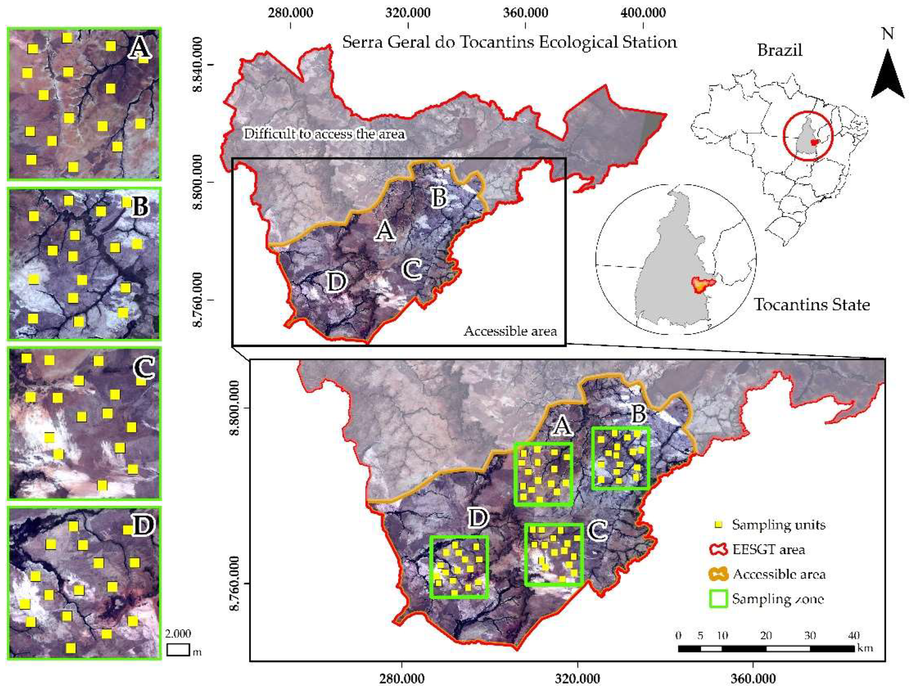
Figure 2.
Overview of fuel sampling. (A) Physiognomy of some sampling areas; (B) Fuel data sampling unit; (C) Sub-samples of surface fuel characterization; (D) Number of samples taken at the beginning (May and June) and end of the dry season (August and September).
Figure 2.
Overview of fuel sampling. (A) Physiognomy of some sampling areas; (B) Fuel data sampling unit; (C) Sub-samples of surface fuel characterization; (D) Number of samples taken at the beginning (May and June) and end of the dry season (August and September).
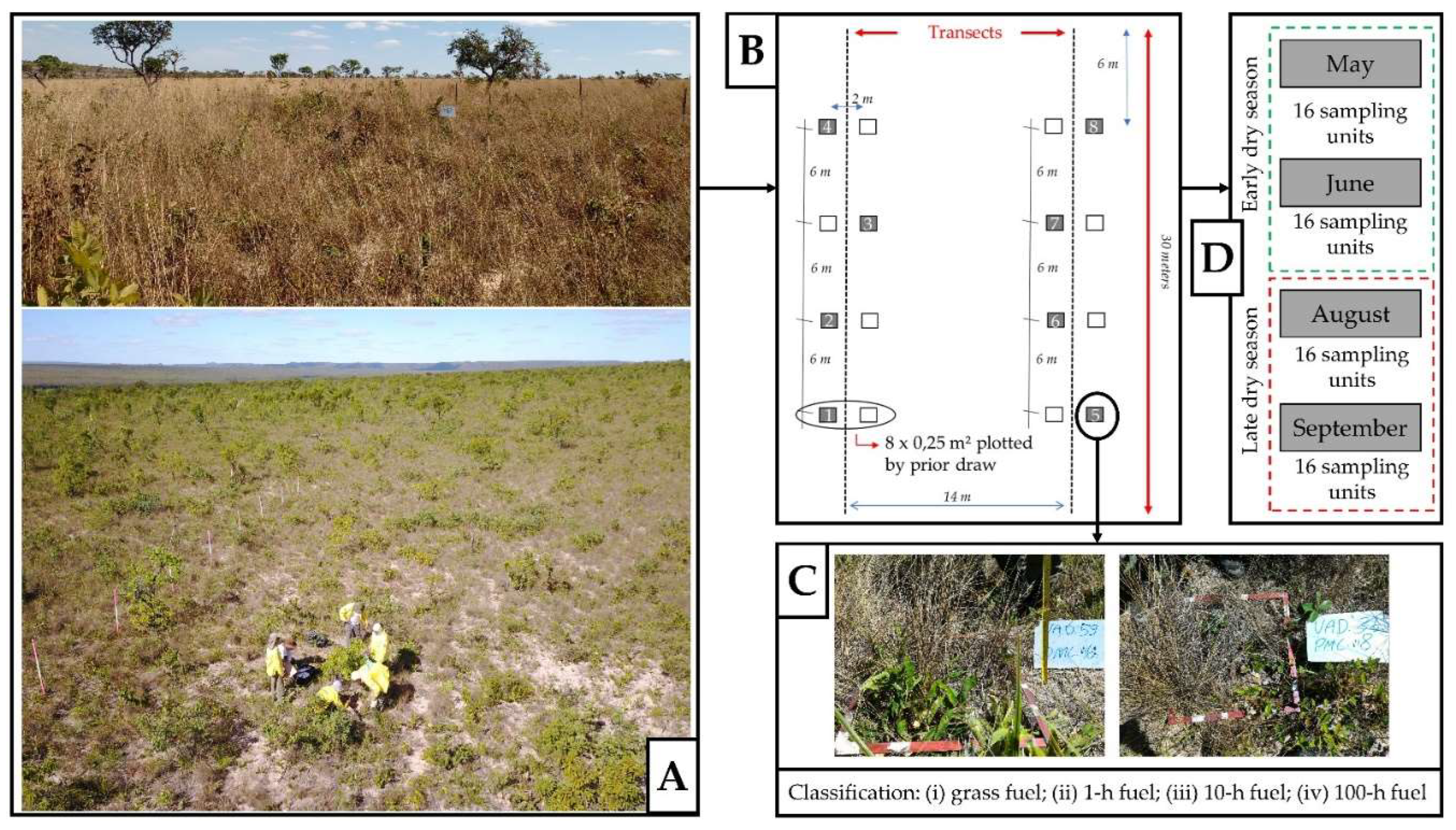
Figure 3.
Flowchart of the methodology applied in this study. R² = coefficient of determination, R²adj = adjusted coefficient of determination, RMSE = root-mean-square error, MAE = mean absolute error.
Figure 3.
Flowchart of the methodology applied in this study. R² = coefficient of determination, R²adj = adjusted coefficient of determination, RMSE = root-mean-square error, MAE = mean absolute error.
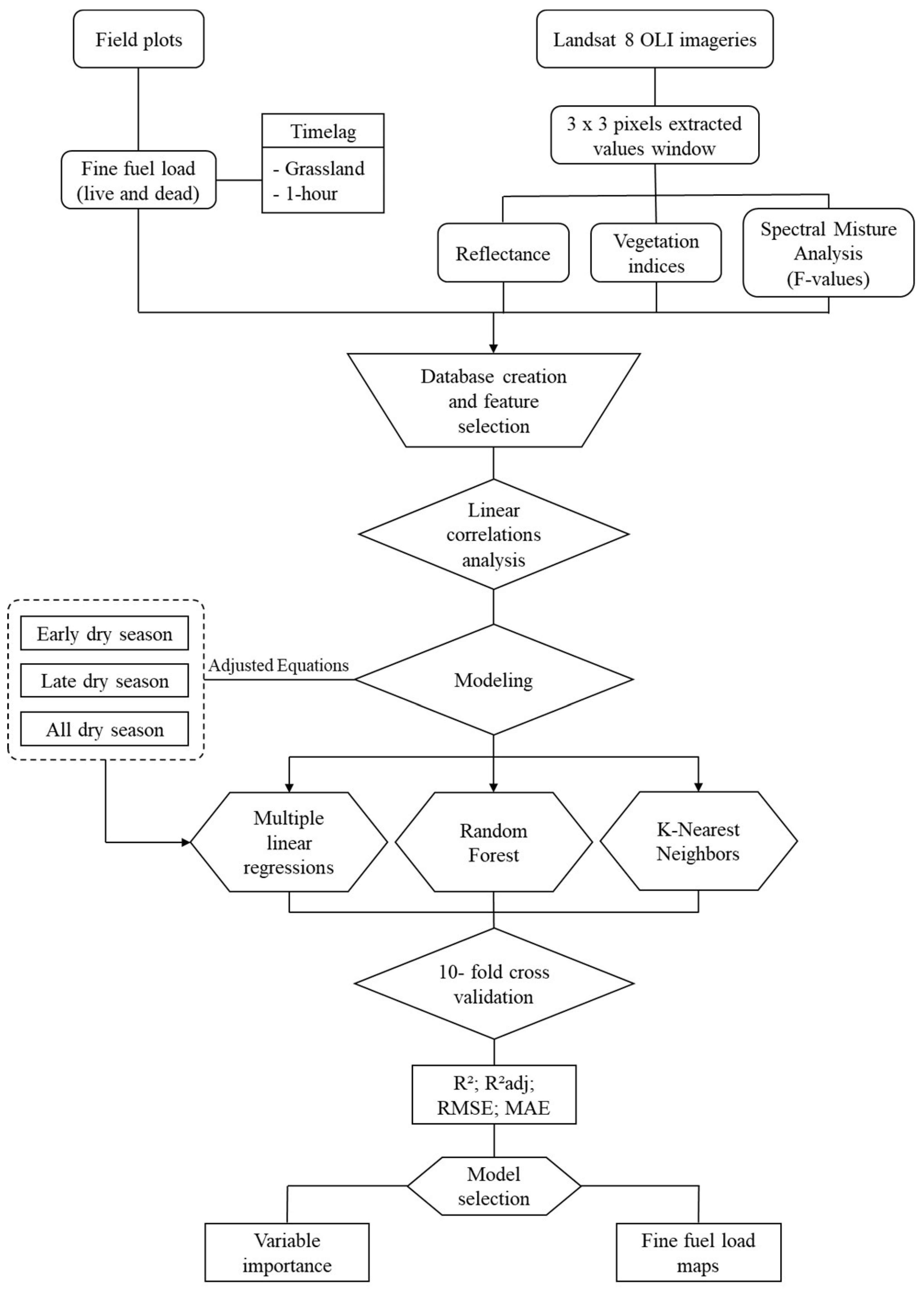
Figure 4.
Fine fuel load mappings performed using the best RF models: (A, B) Estimates for dead grass fuel, (C, D) Estimates for 1-h downed wood debris.
Figure 4.
Fine fuel load mappings performed using the best RF models: (A, B) Estimates for dead grass fuel, (C, D) Estimates for 1-h downed wood debris.
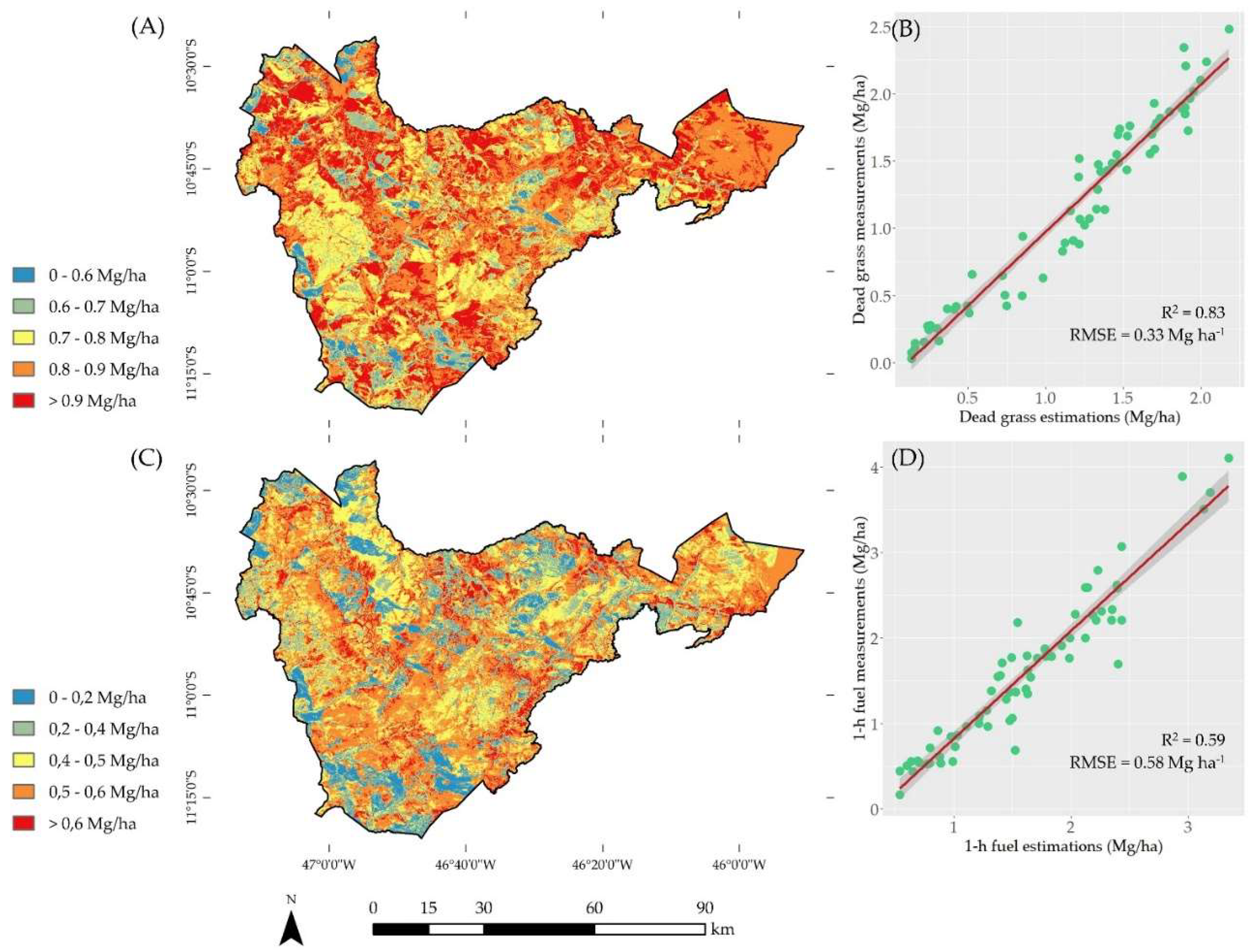
Figure 5.
Fine fuel load mappings were performed using the best RF models: (A, B) Estimates for total fine dead, (C, D) Estimates for total fine fuel.
Figure 5.
Fine fuel load mappings were performed using the best RF models: (A, B) Estimates for total fine dead, (C, D) Estimates for total fine fuel.
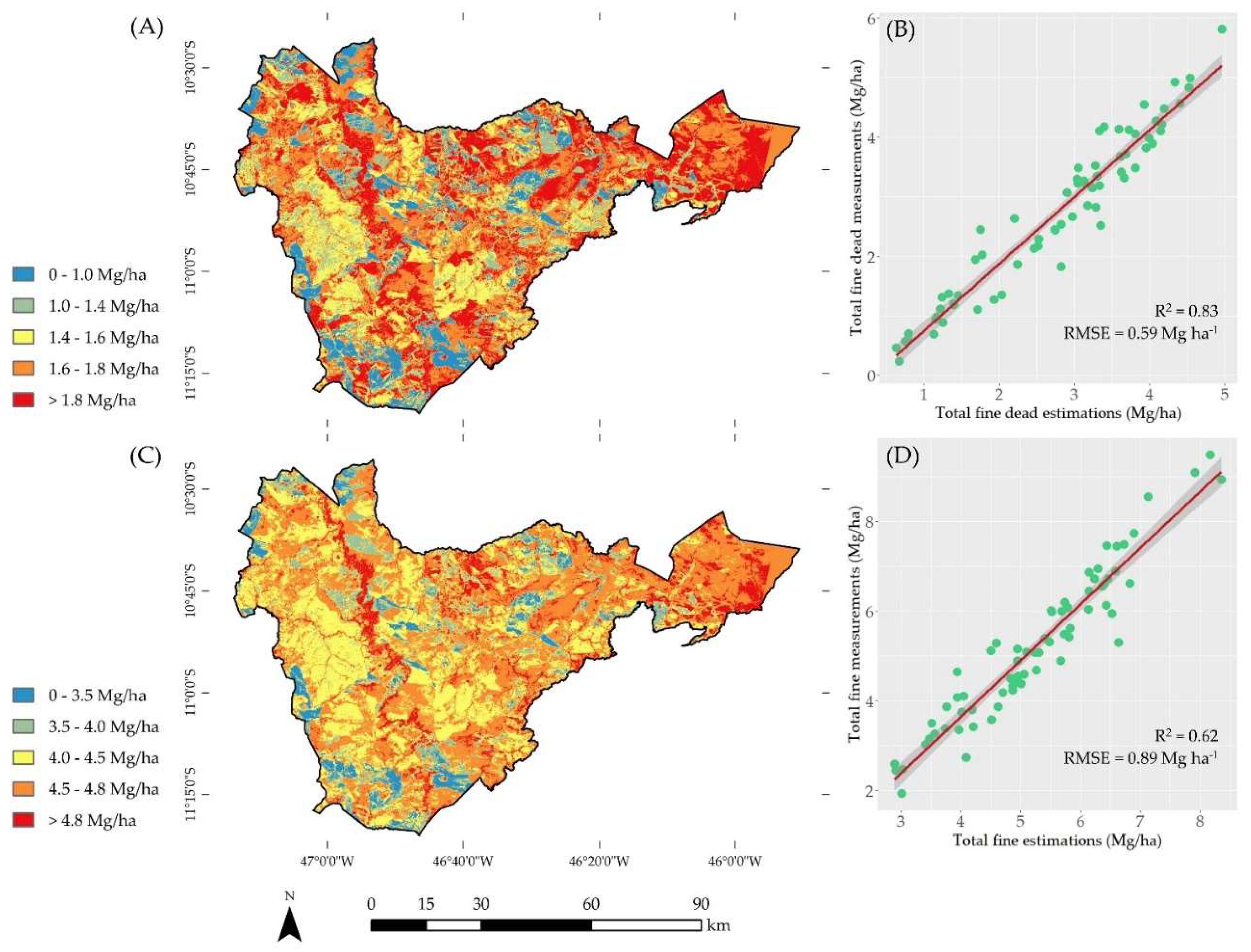
Figure 6.
Importance of the variables of the Random Forest (RF) algorithm models with the best fit for fuel load estimation. a) RF model for dead grass fuel; b) RF models for 1-h downed wood debris; c) RF models for total fine dead fuel; d) RF models for total fine fuel. %IncMSE indicates the increase in the mean squared error in percentage.
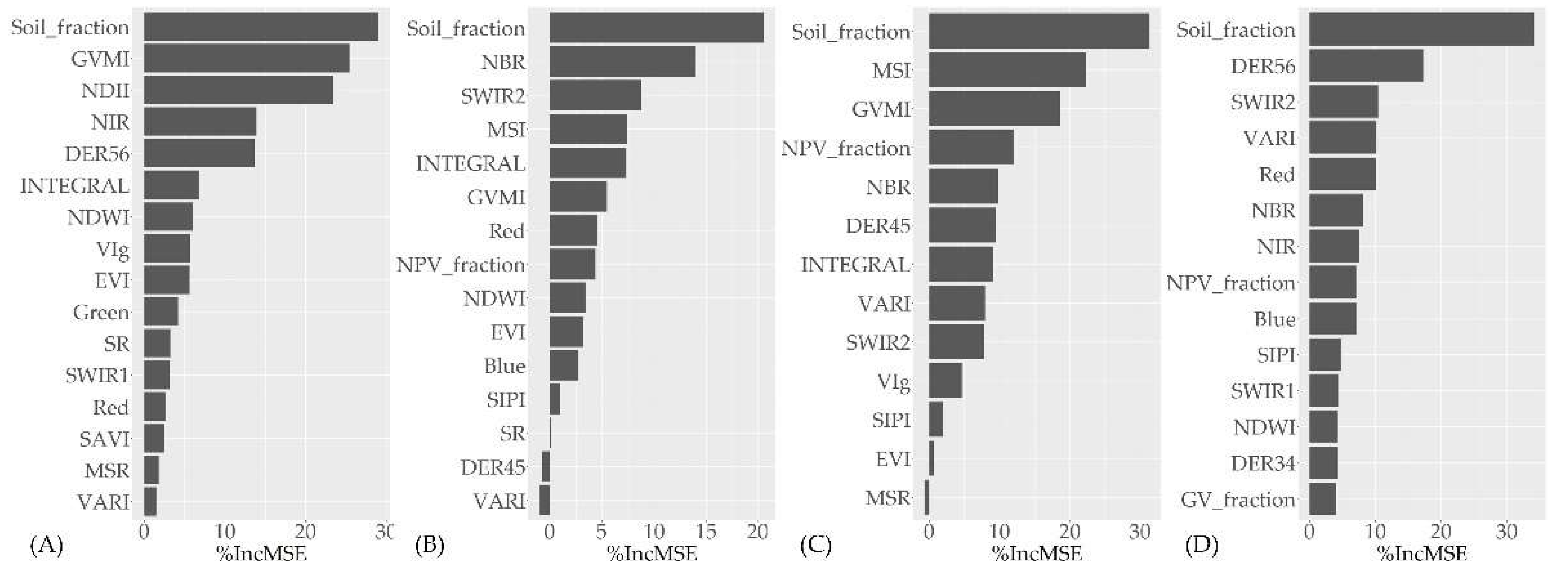
Figure 7.
Fuel condition map consisting of the three sub-pixel fraction images (R: NPV, G: GV, B: Soil) in the Serra Geral do Tocantins Ecological Station for the beginning (May 2017) and end of the dry season (September 2017).
Figure 7.
Fuel condition map consisting of the three sub-pixel fraction images (R: NPV, G: GV, B: Soil) in the Serra Geral do Tocantins Ecological Station for the beginning (May 2017) and end of the dry season (September 2017).
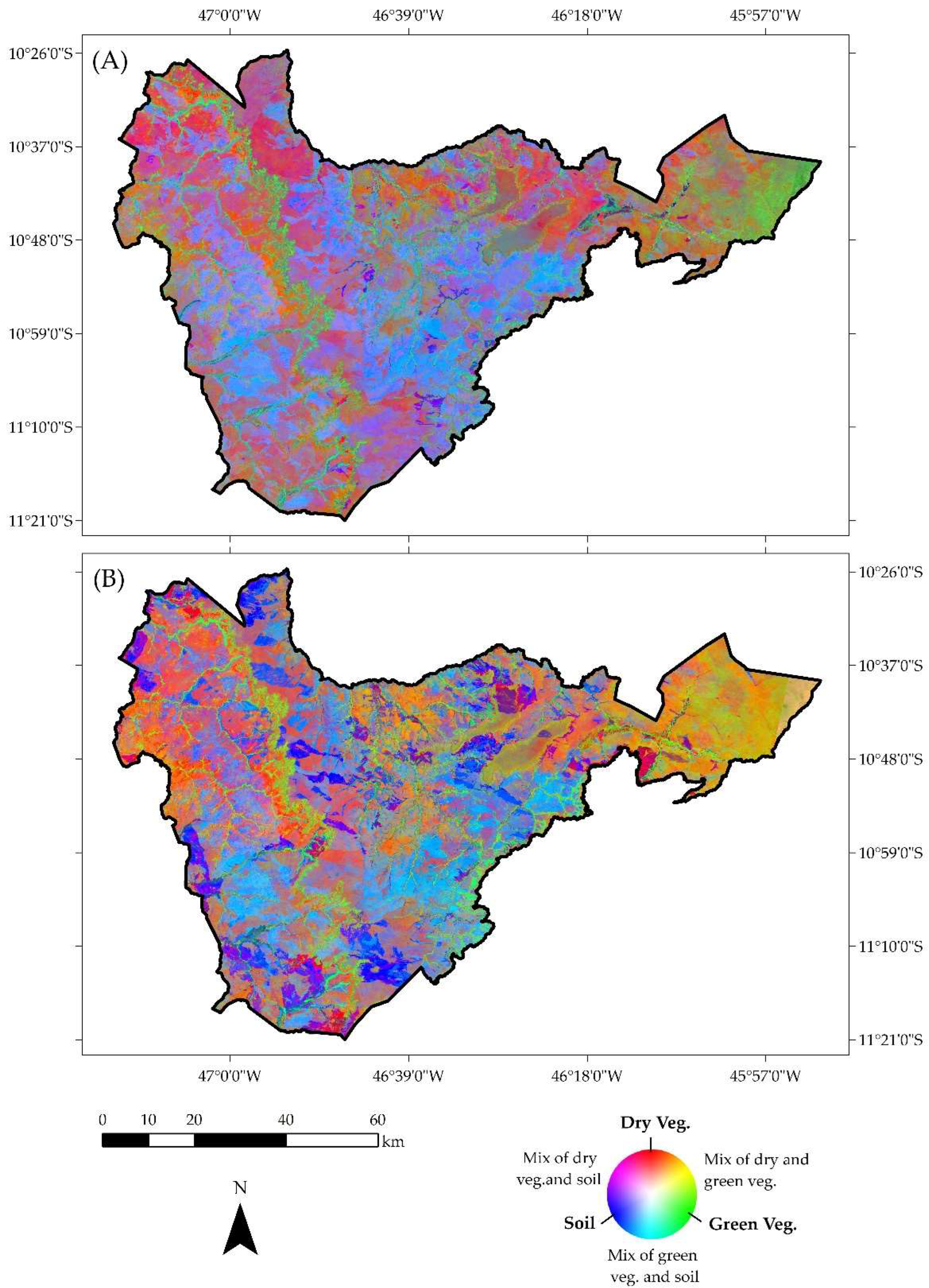

Table 1.
Statistical metrics of the cross-validation of the multiple linear regression models with the best fit for fuel load estimation.
Table 1.
Statistical metrics of the cross-validation of the multiple linear regression models with the best fit for fuel load estimation.
| Per | Estimated fuel (y) | Predictor variables (x) | R² | R² aj | RMSE | MAE |
|---|---|---|---|---|---|---|
| 1 | Dead grass | NPV; Soil; B5: nir; B6: swir 1; B7: swir 2; VARI; SR; SIPI; NDII; MSR; MSI; GVMI; DER56; DER34; | 0.89 | 0.81 | 0.37 | 0.32 |
| 1-h downed wood debris | NPV; Soil; GV; B4: red; B5: nir; B6: swir 1; B7: swir 2; NDVI; VARI; VIgreen; SR; SIPI; SAVI; NDWI; NRR; MSI; MNDWI; DER34; DER23; | 0.81 | 0.55 | 0.45 | 0.37 | |
| Total fine dead (grass + 1-h) | NPV; Soil; GV; B4: red; B5: nir; B6: swir 1; B7: swir 2; VARI; VIgreen; SR; SIPI; SAVI; NDWI; NDII6; NBR; DER45; | 0.92 | 0.84 | 0.49 | 0.40 | |
| Total fine (live and dead) |
NPV; Soil; B2: blue; B4: red; B5: nir; B6: swir 1; NDVI; VARI; VIgreen; SR; SIPI; SAVI; NDWI; NDII6; NBR; MSR; MSI; MNDWI; INTEGRAL; DER45; DER34; DER23; GVMI; | 0.81 | 0.37 | 1.26 | 1.06 | |
| 2 | Dead grass | NPV; Soil; B2: blue; B3: green; B5: nir; B6: swir 1; B7: swir 2; NDVI; VIgreen; SR; NDWI; NDII6; NBR; MSR; MSI; MNDWI; GVMI; EVI; DER56; DER34; DER23; | 0.81 | 0.47 | 0.44 | 0.38 |
| 1-h downed wood debris | NPV; Soil; GV; B2: blue; B3: green; B4: red; B5: nir; B7: swir 2; NDVI; VARI; VIgreen; SR; SIPI; SAVI; NDWI; NDII6; NRR; MSR; MSI; INTEGRAL; GVMI; EVI; DER56; DER45; DER34; DER23; | 0.45 | -1.59 | 1.90 | 1.53 | |
| Total fine dead (grass + 1-h) | Soil; GV; B2: blue; B3: green; B4: red; B5: nir; B6: swir 1; B7: swir 2; NDVI; VARI; VIgreen; SR; SIPI; SAVI; NDWI; NDII6; NBR; MSR; MSI; INTEGRAL; GVMI; EVI; DER56; DER45; DER34; DER23 | 0.64 | -0.72 | 2.24 | 1.98 | |
| Total fine (live and dead) |
Soil; GV; B2: blue; B3: green; B4: red; B5: nir; B6: swir 1; B7: swir 2; NDVI; VARI; VIgreen; SR; SAVI; NDWI; NDII6; MSR; MSI; INTEGRAL; EVI; DER56; DER45; DER34; DER23; | 0.56 | -0.44 | 2.27 | 2.01 | |
| 3 | Dead grass | Soil; B3: green; B4: red; B5: nir; B6: swir 1; VARI; VIgreen; SR; SAVI; NDWI; NDII6; MSR; INTEGRAL; GVMI; EVI; DER56; | 0.78 | 0.72 | 0.36 | 0.31 |
| 1-h downed wood debris | NPV; Soil; B2: blue; B4: red; B7: swir 2; VARI; SR; SIPI; NDWI; NRR; MSI; INTEGRAL; GVMI; EVI; DER45; | 0.57 | 0.45 | 0.62 | 0.51 | |
| Total fine dead (grass + 1-h) | NPV; Soil; B7: swir 2; VARI; VIgreen; SIPI; NBR; MSR; MSI; INTEGRAL; GVMI; EVI; DER45; | 0.73 | 0.66 | 0.75 | 0.62 | |
| Total fine (live and dead) |
NPV; Soil; GV; B2: blue; B4: red; B5: nir; B6: swir 1; B7: swir 2; VARI; SIPI; NDWI; NBR; DER56; DER34; | 0.63 | 0.54 | 1.06 | 0.91 |
Per = Dry season period, where: (1) Early dry season (May and June); (2) Late dry season (August and September); (3) All dry season (May to September).
Table 2.
Statistical metrics used to assess the models generated by the Random Forest algorithm.
| Estimated fuel (y) | Predictor variables (x) | R² | R² aj | RMSE | MAE |
|---|---|---|---|---|---|
| Dead grass | All predictor variables | 0.83 | 0.71 | 0.33 | 0.24 |
| * Soil; B3: green; B4: red; B5: nir; B6: swir 1; VARI; VIgreen; SR; SAVI; NDWI; NDII6; MSR; INTEGRAL; GVMI; EVI; DER56; | 0.83 | 0.78 | 0.33 | 0.23 | |
| 1-h downed wood debris | All predictor variables | 0.59 | 0.30 | 0.58 | 0.44 |
| * NPV; Soil; B2: blue; B4: red; B7: swir 2; VARI; SR; SIPI; NDWI; NRR; MSI; INTEGRAL; GVMI; EVI; DER45; | 0.52 | 0.38 | 0.61 | 0.46 | |
| Total fine dead (grass + 1-h) |
All predictor variables | 0.83 | 0.71 | 0.59 | 0.44 |
| * NPV; Soil; B7: swir 2; VARI; VIgreen; SIPI; NBR; MSR; MSI; INTEGRAL; GVMI; EVI; DER45; | 0.79 | 0.74 | 0.63 | 0.49 | |
| Total fine (live and dead) |
All predictor variables | 0.62 | 0.35 | 0.89 | 0.75 |
| * NPV; Soil; GV; B2: blue; B4: red; B5: nir; B6: swir 1; B7: swir 2; VARI; SIPI; NDWI; NBR; DER56; DER34; | 0.55 | 0.43 | 0.96 | 0.81 |
* Variables selected by stepwise method in multiple linear regression analyses.
Table 3.
K values chosen for each k-Nearest Neighbor algorithm model.
| Estimated fuel (y) | Predictor variables (x) | RMSE value | Chosen K value |
|---|---|---|---|
| Dead grass | All predictor variables | 0.4072 | 5 |
| Stepwise* | 0.4453 | 7 | |
| 1-h downed wood debris | All predictor variables | 0.8183 | 7 |
| Stepwise* | 0.8253 | 9 | |
| Total fine dead (grass + 1-h) | All predictor variables | 1.1051 | 5 |
| Stepwise* | 1.1233 | 9 | |
| Total fine (live and dead) |
All predictor variables | 1.6060 | 7 |
| Stepwise* | 1.6136 | 13 |
* Variables selected by stepwise method in multiple linear regression analyses.
Table 4.
Statistical metrics used to assess the models generated by the k-NN algorithm.
| Estimated fuel (y) | Predictor variables (x)1 | R² | R² aj | RMSE | MAE |
|---|---|---|---|---|---|
| Dead grass | All predictor variables | 0.68 | 0.45 | 0.37 | 0.30 |
| Stepwise* | 0.61 | 0.49 | 0.41 | 0.34 | |
| 1-h downed wood debris | All predictor variables | 0.34 | -0.13 | 0.74 | 0.61 |
| Stepwise* | 0.31 | 0.11 | 0.76 | 0.63 | |
| Total fine dead (grass + 1-h) | All predictor variables | 0.54 | 0.21 | 0.92 | 0.78 |
| Stepwise* | 0.49 | 0.37 | 0.98 | 0.84 | |
| Total fine (live and dead) |
All predictor variables | 0.38 | -0.07 | 1.43 | 1.23 |
| Stepwise* | 0.30 | 0.12 | 1.53 | 1.31 |
* Variables selected by stepwise method in multiple linear regression analyses. 1 Same predictor variables are shown in Table 2 for RF models.
Disclaimer/Publisher’s Note: The statements, opinions and data contained in all publications are solely those of the individual author(s) and contributor(s) and not of MDPI and/or the editor(s). MDPI and/or the editor(s) disclaim responsibility for any injury to people or property resulting from any ideas, methods, instructions or products referred to in the content. |
© 2023 by the authors. Licensee MDPI, Basel, Switzerland. This article is an open access article distributed under the terms and conditions of the Creative Commons Attribution (CC BY) license (http://creativecommons.org/licenses/by/4.0/).
Copyright: This open access article is published under a Creative Commons CC BY 4.0 license, which permit the free download, distribution, and reuse, provided that the author and preprint are cited in any reuse.


