
Submitted:
20 September 2023
Posted:
22 September 2023
You are already at the latest version
Abstract
The present work sets out the evaluation of composite laminates through optimization objective functions. Genetic Algorithms (GA), as well as Simulated Annealing (SA), were performed in order to determine the optimal ply orientations of a fiber-reinforced polymer laminate for three given load cases: 1) in-plane loads, 2) combined moments, and 3) in-plane loads and combined moments. It searches the optimal orientation layup, which fulfills at the same time both the maximum strain criterion and the Tsai-Wu failure criterion. Construction of an objective function based on the strains and the stresses involves a minimization process to deformations and a maximization of the safety factor. For the first load case, the initial solution is [±45/0/90/±45]s, and the best solution is [(45/135)2/452]s. For the second load case, [-45/45/45/-45/0/90]s is the initial layup sequence, then the best solution obtained is [(45/-45)2/452]s, where plies at 0° and 90º are not necessary even when axial loads are applied. For the third study case, the original layup sequence is [0/45/-45/45/0/90]s; meanwhile, the best solution calculated is [21/24/145/140/45/49]s. An interesting observation is that each pair of layers has a 5º gap. The simulations show that the qualitative results from the GA are better than the SA, but with a significantly higher computational cost. These kinds of computational tools are expected to be used as a reference guide for an optimal fiber configuration with respect to the common orientations used when composite laminates are designed for a structural application.
Keywords:
composite material
; laminates orientation
; optimization
; simulated annealing
; genetic algorithm
1. Introduction
For the design of a composite material laminate, it is essential to consider several factors to satisfy the engineering and financial requirements. The first decision drivers are the raw materials with which the composite will be manufactured. Reinforcement and matrix will determine together the end material's physical, chemical, and mechanical properties. However, the number of plies, orientation, and stacking sequence will define the performance of the final structure to resist the applied loads [1].
One of the unique characteristics of composites is that mechanical properties can be tailored to resist specific load conditions. The fibers are stronger in their longitudinal axis. Therefore, the design aims to orient as many layers as possible in the direction of the applied stress. As layers are stacked through the thickness at different orientations, hundreds of combinations can exist that could fulfill the mechanical purpose [2,3].
In the case of uniaxial or biaxial stress, selecting plies' orientation can be easy, which can be accomplished by experimentation or computer simulation. However, as the stress state becomes triaxial due to combined loads and moments, it becomes a real challenge requiring a more exhaustive analysis of the orientation and stack-up sequence of the constituent plies. The common practice on composite structures design suggests the implementation of quasi-isotropic configuration, [0/90/+-45], with [50-10-40] volume proportions, respectively. The goal is to have an isotropic and balanced material which could fulfill the most common load cases but is not optimized.
The optimization of composite laminates contemplates two main goals: 1) minimization of weight [4,5] and 2) maximization of the load-carrying capacity [1,6]. The optimization of the specific strength is translated into a reduction of raw materials, manufacturing tasks, and laps, and, therefore, cost improvement [7].
These two goals have motivated the use of several optimization methods (gradient-based, direct search, heuristics, and hybrid), turning the composite's structural design into a more systematic and well-defined task, less dependent on the designer and more focused on the 5material performance [6,8,9].
For composite laminate structures, two stages need to be accomplished. First, in constant stiffness consideration, the composite part is treated as a single element, and the goal is to find an optimal stacking sequence uniform for the entire structure. Second, in variable stiffness consideration, the composite part is partitioned into several elements, each with a particular fiber orientation and stacking sequence [10,11].
For the first stage, direct search methods have been employed due to their advantage of not requiring information on the gradient and for not being sensitive to the initial search point; founding their results by using function values of preceding iterations. These methods strongly portray non-linear and noisy search spaces [12,13,14,15]. Also, the methods cover more uniformly ample search space; due to their inherent stochasticity, it escapes more easily from local optima. In this category, two powerful tools are found, genetic algorithms (GA) [16,17,18,19,20,21] and simulated annealing (SA) [16,22,23,24,25,26]. Newer and more sophisticated optimization algorithms are reported elsewhere [27,28]. However, our goal is to present a rigorous procedure based on strain and safety criteria to support the design of laminated material.
The laminates' orientation affects the composite material's mechanical behavior in several ways. Laminates oriented in the same direction as the applied load will experience more significant stiffness and strength in that direction. In contrast, laminates oriented perpendicular to the applied load will experience higher flexibility and toughness in that direction. Since the optimal orientation of laminates in a composite material depends on the specific application and the desired mechanical properties, this work aims to evaluate the optimization methodologies based on Genetic Algorithm and Simulated Annealing to support the design of fiber-reinforced laminates and define rigorous criteria to decide if the standard practices' orientations guarantee at the same time the maximum strain and Tsai-Wu safety factor criteria.
This paper presents a numerical investigation to evaluate two different optimization algorithms applied to composite structures. The model description takes place in the first section by defining the corresponding physical and mathematical considerations. Then, in the second section, the problem formulation is set to calculate the optimal orientations design in a stacking sequence which fulfills at the same time both the maximum strain criterion and the Tsai-Wu failure criterion. The third section shows the results for three different study cases. Finally, conclusions are cited regarding the performance of the Genetic Algorithm (GA) and Simulated Annealing (SA) as optimization techniques for calculating fiber-reinforced composites loaded under consideration of classic laminate theory.
2. Methodology
2.1. Model description
The optimization is carried out by assuming considerations that allow formulating the corresponding mathematical model which describes the physical process. Such suppositions are listed below:
- All laminas have an orthotropic behavior, which implies that the stiffness matrix is reduced to a 6 X 6 matrix system with 21 independent elastic constants.
- The laminate thickness is small compared to the other dimensions, implying that all laminas are restricted to an in-plane stress state, so stresses in the z-direction are negligible. This means that the stiffness matrix becomes a 3 X 3 matrix system with 4 independent elastic constants.
- There is a perfect bond between different laminas. Here it is assumed that all of them are subjected to the same midplane strain.
- Strain distribution in the laminate thickness is linear so that the response of each lamina depends on its relative location regarding the midplane of the laminate.
- All laminas are macroscopically homogeneous and have a linear-elastic behavior. This means that mechanical properties do not depend on the spatial location.
- The laminate works under a constant stiffness principle. This means that the stiffness is the same in the entire domain of the laminate and no discontinuity of each ply is allowed.
- Residual stresses derived from the curing process are negligible.
2.2. Theory of laminates
This classical theory is based on the assumptions deployed above for a thin-shell structure so that the mechanical properties of a composite material are evaluated by considering in-plane stress conditions. The generalized Hooke's equation for an orthotropic, three-dimensional composite material gives a linear relationship between stress and strain as follows:
and, according to the assumptions defined above, the equation that describe the behavior of a lamina in an orthotropic composite material is given by:
Where elements constitute the material's stiffness matrix and depend on the material properties (E1, E2, G12, and ν12) in the principal directions.
A laminate composed of laminas of orthotropic composite material (Figure 1) is expected to be loaded with in-plane forces and moments that will produce strains and curvatures, respectively [29,30]. The resultant of forces and moments acting on the laminate can be obtained by integration of stresses along the thickness (z) according to the equations (Eqs. (3) and (4), respectively.
Note that (i = x, y, xy) are the forces and the moments, both, per unit length. These terms are related to the strains and curvatures by means of the stiffness of the laminate.
The representation of such properties in terms of the ABD matrix is:
Coefficients related to the extensional stiffness elements are evaluated according to:
the coupling extension bending components are calculated as:
and the bending stiffness elements are evaluated as
where are the elements of the stiffness matrix of a lamina expressed in the laminate's coordinate axes, indicates the relative position of a layer respect to the midplane of the laminate, and is the orientations angle associated to the stacking sequence.
2.3. Problem formulation
The goal is to obtain the optimal orientations design in a stacking sequence which fulfills at the same time both the maximum strain criterion and the Tsai-Wu failure criterion. Thus, an objective function is proposed, based on the strains and the stresses that involves a minimization process to deformations and a maximization to the safety factor. The optimization process is carried out on a symmetric laminate, so it is enough to consider half of the plies, and by the nature of this kind of laminate, values will be zero.
As a benchmark, a weakest-link failure approach was adopted regarding the first ply of the laminate, which is subjected to the highest stresses. The Tsai-Wu safety factor is maximized. The design variables are the orientations of the layers, and the number of plies and ply thickness are kept constant. To assure the static strength of the laminate, the safety factor of all plies is also calculated.
The Tsai-Wu failure criterion indicates when a ply subjected to an in-plane stress condition will fail. It happens if and only if the following expression is satisfied:
where , , and are the first ply stresses obtained from Eq. (2) The terms can be evaluated as: ,, , , , and .
Specifically, the Tsai-Wu safety factor is defined as:
The coefficients of Eq. (10) are evaluated as: , , and .
Notice that there is an implicit dependence of on the orientation of a ply as the stresses depend on the stiffness matrix which is angle and thickness-dependent.
In a composite material of different plies with non-periodic orientations and located at equidistant positions from the middle, the objective function is constituted by the contributions of the safety factor of all plies in the stacking sequence according to:
To maximize the objective function, it is necessary to include the constraints that complement the safety factor criteria. The optimization problem can be announced as:
where is the vector of constant parameters, such as the material properties which do not change during the optimization process, is the orientation angle of each ply that is allowed to vary in the range .
3. Results and discussion
3.1. Application cases
3.1.1. In-plane loads
The study case 1, with the aim to verify the robustness of both optimization algorithms was a composite laminate under in-plane loads. The shear load per unit length is higher than the axial loads and . Shear load is twice the axial loads per unit length. This load case is considered as reference laminate the following configuration: [±45/0/90/±45]s. This layup is intended to have most of the plies with a 𝜃= 45º to increase the shear strength and add a couple of 0º and 90º layers to improve axial stiffness. The reference laminate has SF = 1.57 at its weakest ply and an objective function value of -3.5362 (see Table 1).
Figure 2 and Figure 3 show, respectively, i) the results for objective function values and ii) number of evaluations of objective function. From Figure 2, it can be highlighted that GA is able to find solutions with the same value of objective function, -7.2200, which is a clear indicator of the good stability of GA with respect to the input parameters (see Table 2). The results for SA fall in a range between -5.7274 and -6.9932, revealing a lower stability of the algorithm and its drawback to escape from local optimum (see Table 3). Nonetheless, solutions found by SA are clearly superior to the initial solution.
Comparing both algorithms, the value of the objective function by SA is lower than GA, but has a high variability. GA average function value is -7.2200 and a variability coefficient of 7.14% (see Table 2). The SA has an average function value of -6.3996 and a variability of 5.8% (see Table 3). The dispersion for the GA is despicable compared with the ones obtained by SA. Although SA solutions are satisfactory, these results show lower performance for the in-plane load condition than GA solutions.
Execution time required to obtain the optimal solution using SA is lower than GA. SA time gaining is almost twice fast as GA. By nature, GA needs more computational time to compute optimal solutions.
There are no significant differences between the layup configuration for the worst and best solution for GA solutions. Those solutions keep the same proportion of 8 plies with orientation near = 45º and 4 plies with near = 135º (see Table 2). These results show the high stability of the algorithm. A similar trend is found for SA solutions, but it is probable that this algorithm got stuck in a local optimal before it can improve the orientation values. In this study case, the initial solution is in the form of [±45/0/90/±45]s, and the best solution obtained is [(45/135)2/452]s, which means that plies at 0º and 90º are not necessary, even when there are axial loads applied (see Table 3). Due to the magnitude and ratio of loading case, mainly shear, a ±45° based configuration is sufficient to grant the laminate strength. Solutions obtained by both algorithms, according to the optimization criterion and based on the SF of the weakest ply, represent better configurations than the reference laminate, however GA solutions remain superior.
3.1.2. Combined moments
The study case 2, composite laminate was charged combining bending and torsion moments. In this study case, the torsion moment has the highest magnitude. Initial solution of the laminate has a layup sequence as follows: [-45/45/45/-45/ 0/90]s. Layup sequence has ±45 plies at the bottom and the top of the laminate to increase the in-plane shear stiffness as shown in Table 4. This configuration has a SF of 0.7240 in the weakest layer and an objective function value of -2.5567. Because one of the layers has a SF that does not satisfy the Tsai-Wu criterion, the objective function value, with this layup sequence, was penalized by diminishing its value.
From Figure 4, GA found 5 local optimal solutions with the following objective function values: -5.4950, -5.5206, -5.6228, -5.6230 and -5.6532. It can be highlighted that only one execution results in a value of -5.4950, meanwhile 16 executions have objective functions values below -5.6.
The response of GA to input parameters is stable, by obtaining solutions that asymptotically approach one objective function value. The average value of the objective function in this study case is -5.0672 with a variation coefficient of 0.8824%.
Different objective function values were computed in all solutions for the SA algorithm. This trend showsSA's difficulty in escaping from local optima and converge. SA objective values oscillate between -3.3396 and -5.3112, with an average value of -4.4810 and a coefficient of variation of 11.43%. Despite most SA solutions being satisfactory, statistical data show a lower stability and performance compared to GA.
From Figure 5, the GA required ten times more evaluations to find the optimal solution than SA. The GA needed to process at least 17200 evaluations, meanwhile SA could afford it with 3152 evaluations. Comparing the computational cost, the SA obtained a solution in an average time of 21.60 s, while GA took 35.51 s to find a solution.
As shown in Table 5 the best and worst solution from the optimization algorithms are proposed with 45º and 135º (or -45º) lamina. The position of the (-45º) laminate has a considerable impact, because although most of the solutions satisfy the SF, the objective function value depends on the position of this particular orientation.
With the results shown in Table 6, solutions proposed by the SA are better than the reference laminate. However, SA solutions have a lower value of objective function, which is noticeable on the weakest lamina showing a lower SF. The worst solution proposed by SA has a lamina with a SF < 1, which does not fulfill the Tsai-Wu criterion. Even when SA solutions trend to lamina with = 45° and = -45º, it is possible that for those solutions the algorithm got stuck in a local optimum.
In this study case, the reference solution has [-45/45/45/-45/0/90]s as a layup sequence. The best solution obtained is of the type [(45/-45)2/452]s. For this load case, it is also unnecessary to add plies at = 0° and = 90º, even when there are axial loads applied. This load case shows that optimization algorithms can discard "common practices layups" in which plies with orientation of 0° and 90° are always added in the laminate configuration
3.1.3. In-plane loads and combined moments
In the study case 3, composite laminate was loaded with in-plane loads and combined moments. Typically, this is the loading case for which most composite plate structures are designed. For this case, the reference layup sequence is as follows: [0/45/-45/45/0/90]s, as depicted in Table 7. The layup sequence was selected by placing the 0º and 45º plies near the laminate's surface to increase the bending and torsion stiffness. Plies at 0º and 90º are near the neutral to strengthen the imposed membrane loads. This composite has an average objective function value of -0.2887 and a SF of 0.6940 on its weakest ply. As it can be seen, the value of the objective function for this solution is significantly reduced because one of its plies does not comply with the Tsai-Wu criteria.
Considering the evolution of the objective function for the optimal solution, all GA solutions have a higher value, nonetheless, SA solutions are very close to them. Both algorithms obtained better quality solutions than the reference one, however, SA showed more variability. The average value for the objective function by GA is -2.0271 with a coefficient of variation of 3.30%. The average value for the objective function by SA is -1.7695 with a coefficient of variation of 17.69%.
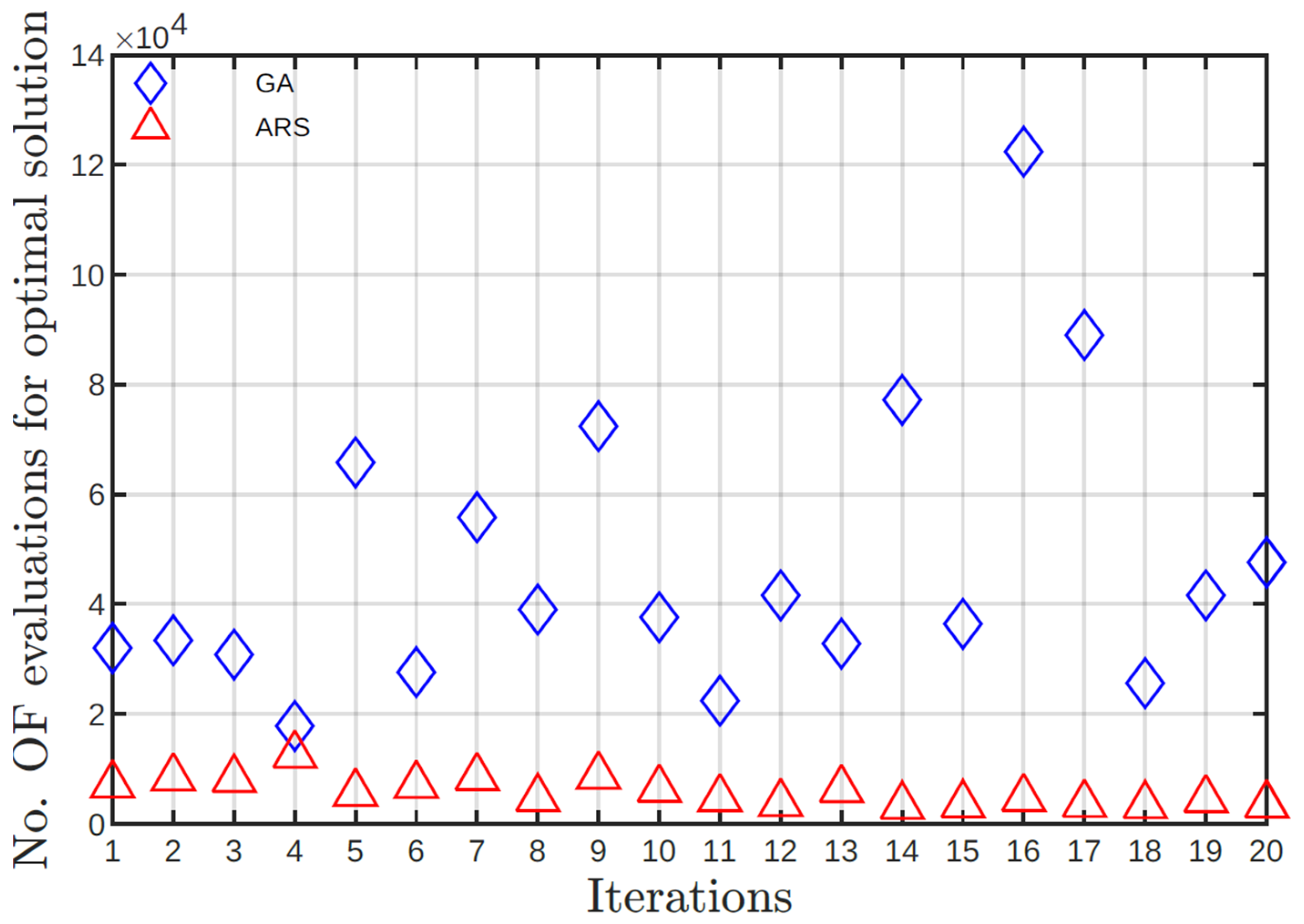
Similarly to case 1 and 2, the GA required a higher number of evaluations of the objective function compared to SA. For case 3, GA required at least 17800 function evaluations with a maximum of 122400. In contrast, SA required at least 3197 evaluations with a maximum of 12503. The number of evaluations for GA is almost one order of magnitude bigger than SA. The number of evaluations needed to find the optimal solution is reflected in the computational time. In this sense the SA had a better solution time, from 8.43 seconds to 29.98 seconds, while the GA spent from 21.67 seconds to 126.65 seconds. The difference in computational time is evident.
In this study case, GA solutions promote layers near = 22° and = 24° at the surface, as it can be seen in Table 8. Plies from 3rd to 6th have complementary angles. For example, the 3rd layer of the best solution has = 145º, and the same layer of the worst solution has = 27º.
It can be noticed in Table 8, that the GA solution with the worst value of objective function has at its less resistant layer (1st ply) a SF superior to the less resistant layer of the best solution (ply 10th), which is at its strength limit. Nonetheless, this last solution is considered of better quality for the optimization criterion employed.
The 3rd and 4th layers of the solution with the highest value of objective function, are those that cause this increment. Both solutions satisfy the Tsai-Wu criterion and represent better options than the reference one (see Table 8).
On the other hand, it can be noticed in Table 9 that SA proposes similar orientation angles for the first four layers in its best solution compared with GA. The worst solution by SA has the lowest value of the objective function. This solution presents a ply with a SF = 0.93, which does not comply with the Tsai-Wu criterion (see Table 9). It can be noticed that the orientation angles for the best and worst SA solutions are very different. It can be implied that the SA algorithm could be stuck in a local optimum, being unable to improve the orientation angles, raising the value of the objective function and, therefore, being penalized.
Although the lower performance to find solutions for the considered optimization criterion, the SA algorithm fulfills to obtain on 18 of 20 executions, solutions that were not penalized and which are considered better than the reference layup.
In this study case the original layup sequence is [0/45/-45/45/0/90]s, meanwhile the best solution proposed by the optimization algorithms is [21/24/145/140/45/49]s. An interesting observation is that if the layers are regrouped in pairs, each orientation has a gap of 5° . In this study case, the optimal solution shows that the inclusion of plies with = 0º or 90º is not mandatory. Each load case can have a related layup sequence, where the correct angle orientation can significantly improve the performance of the composite structure.
Figure 6.
Objective function values for GA and SA for study case 3.
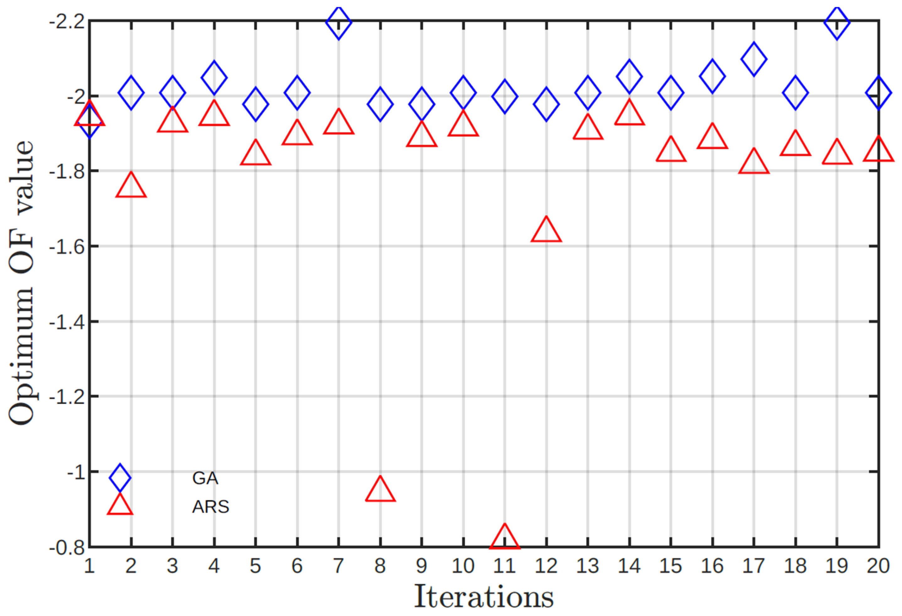
Figure 7.
Number of evaluations for GA and SA for study case 3.
4. Conclusions
This paper studied the performance of Genetic Algorithm (GA) and Simulated Annealing (SA) as optimization techniques for calculating fiber-reinforced composites loaded under consideration of classic laminate theory. The main objective is to obtain the optimal orientation layup, which fulfills at the same time both the maximum strain criterion and the Tsai-Wu failure criterion for different loading cases.
GA presented a good performance but with a higher computational cost concerning SA. In all study cases, GA found solutions that overpass the expectations of the initial (reference) solution. GA also showed great stability, any input data do not influence it, and in most cases, it was able to find at different executions, convergence solutions.
SA was able to find optimal solutions with a good value of objective function. Nonetheless, it is strongly influenced by the input parameters. The variability is higher than GA, but it can obtain solutions in a very short time. SA optimized solutions are also always better than the proposed ones.
GA solutions have a higher value of objective function than SA. SA has a higher variability in the results with respect to GA, which suggests a more limited capability of the algorithm to escape from local optima.
For the first load case, in-plane loads, the initial solution is in the form of [±45/0/90/±45]s, and the best solution obtained by both optimization algorithms is in the form of [(45/135)2/452]s. For the second load case, combined moments, [-45/45/45/-45/0/90]s is the initial layup sequence, then the best solution obtained provided by both optimization algorithms is in the form of [(45/-45)2/452]s. For the third study case, combined moments, the original layup sequence is [0/45/-45/45/0/90]s, meanwhile the best solution calculated by the optimization algorithms is [21/24/145/140/45/49]s. In all three cases, plies at 0º and 90º are unnecessary even when applied axial loads.
Both techniques, GA and SA, have proven advantages and disadvantages. However, both algorithms found better solutions than the reference ones.
It is also highlighted that layup solutions rarely contain plies oriented near the common practice angles in all three study cases. With this study, a slight variation in the orientation angles could significantly impact mechanical performance. Exploration of these non-common angles would be challenging without tools such as GA or SA optimization techniques.
The use of optimization techniques can improve design time and cost. Further work will consider an experimental comparison between the reference layup versus the optimal layup calculated.
Author Contributions
Conceptualization, resources, writing—original draft preparation and investigation, M.T.A.; Formal analysis and investigation, A.B.V.; Calculations and discussion, S.P.-G. M.T.A. E.H. A.B.V.; Writing—review and editing, E.A.F.-U.; Methodology, visualization and investigation, S.P.-G. M.T.A. E.H. A.B.V. P.O. All authors have read and agreed to the published version of the manuscript.
Data Availability Statement
This study does not report any data.
Acknowledgments
Authors acknowledge support from CONACYT-AEM Fund for Research and Development of Space Activities, Grant 275783, from CONACYT-SEP Mexican Basic Science Research, Grant 257458 and CONACYT Research Fellow Program.
Conflict of Interest
The authors declare no conflict of interest.
References
- CS Lee JH Park, JH Hwang and W Hwang. Stacking sequence design of composite laminates for maximum strength using genetic algorithms. Composite Structures, 52:217–31, 2001. [CrossRef]
- FS Almeida and AM Awruch. Design optimization of composite laminated structures using genetic algorithms and finite element analysis. Composite Structures, 88:443–54, 2009. [CrossRef]
- L Aydin and HS Artem. Multiobjective genetic algorithm optimization of the composite laminates as a satellite structure material for coefficient of thermal expansion and elastic modulus. 4th International Conference on Recent Advances in Space Technologies (RAST), 2009.
- FO Sonmez and M Akbulut. Optimum design of composite laminates for minimum thickness. Computers and Structures, 86:1974–1982, 2008. [CrossRef]
- MA Akgu ̈n RT Haftka, B Liu and A Todoroki. Permutation genetic algorithm for stacking sequence design of composite laminates. Computer methods in applied me- chanics and engineering, 186:357–372, 2000. [CrossRef]
- M Abdalla S Setoodeh and Z Gu ̈rdal. Design of variable-stiffness laminates using lamination parameters. Composites Part B Engineering, 37:301–09, 2006. [CrossRef]
- M Zhou DC Barton D Liu, VV Toporov and OM Querin. Optimization of blended composite wing panels using smeared stiffness technique and lamination parameters. 51st AIAA/ASME/ASCE/AHS/ASC Structures, Structural Dynamics, and Materi- als Conference, 51, 2010.
- M Abouhamze and M Shakeri. Multi-objective stacking sequence optimization of laminated cylindrical panels using genetic algorithm and neural networks. Composite Structures, 81:253–63, 2007. [CrossRef]
- E Lund. Buckling topology optimization of laminated multi-material composite shell structures. Composite Structures, 13:158–167, 2009. [CrossRef]
- D Pasini H Ghiasi and L Lessard. Optimum stacking sequence design of composite materials part i: Constant stiffness design. Composites Structures, 90:1–11, 2009. [CrossRef]
- D Pasini and L Lessard H Ghiasi, K Fayazbakhsh. Optimum stacking sequence design of composite materials part ii: Variable stiffness design. Composites Structures, 93:1– 13, 2010. [CrossRef]
- SS Rao. Engineering Optimization: Theory and Practice. John Wiley & Sons, 4th edition, 2009.
- S Ferrero M Codegone, G Chiandussi and F Varesio. Comparison of multiobjective optimization methodologies for engineering applications. Computers and Mathematics with Applications, 63:912–942, 2012. [CrossRef]
- A Osyczka. Multicriteria optimization for engineering design. Design Optimization, 1:193–227, 1985.
- RT Haftka Z Gürdal and P Hajela. Design and optimization of laminated composite materials. 1999.
- M Asjad S Khan and A Ahmad. Review of modern optimization techniques. Inter- national Journal of Engineering Research Technology, 4:984–988, 2015.
- RT Haftka G Soremekun, Z Gürdal and LT Watson. Composite laminate design optimization by genetic algorithm with generalized elitist selection. Computers & Structures, 79:131–143, 2001. [CrossRef]
- Z Gürdal VB Gantovnik and LT Watson. A genetic algorithm with memory for op- timal design of laminated sandwich composite panels. Composite Structures, 58:513– 520, 2002. [CrossRef]
- YC Hsu SF Hwang and Y Chen. A genetic algorithm for the optimization of fiber angles in composite laminates. Journal of Mechanical Science and Technology, 28:3163– 3169, 2014. [CrossRef]
- V Hoo-Fu HC Vu-Do T Vo-Duy, D Duong-Gia and T Nguyen-Thoi. Multi-objective optimization of laminated composite beam structures using nsga-ii algorithm. Composite Structures, 168:498–509, 2017. [CrossRef]
- L Nolle T El-Mihoub, A Hopgood and A Battersby. Hybrid genetic algorithms: A review. Engineering Letters, 13, 2006.
- R Rutenbar. Simulated annealing algorithms: An overview. IEEE Circuits and Devies Magazine, 5:19–26, 1989. [CrossRef]
- M Akbulut and FO Sonmez. Design optimization of laminated composites using a new variant of simulated annealing. Computers Structures, 89:1712–1724, 2011. [CrossRef]
- Erdal and FO Sonmez. Optimum design of composite laminates for maximum buckling load capacity using simulated annealing. Composite Structures, 71:45–52, 2005. [CrossRef]
- M Kumar V Kumar-R Kumar BB Nayak, S Kundu and KP Shivam. Parametric optimization in drilling of gfrp composites using desirability function integrated simulated annealing approach. Materials Today: Proceedings, 44:1983–1987, 2021. [CrossRef]
- ARM Rao and N Arvind. Optimal stacking sequence design of laminate composite structures using tabu embedded simulated annealing. Structural Engineering and Mechanics, 25:239–268, 2007. [CrossRef]
- F Reguera and VH Cortinez. Optimal design of composite thin-walled beams using simulated annealing. Thin-Walled Structures, 74:71–81, 2016. [CrossRef]
- MS Azqandi. A novel hybrid genetic modified colliding bodies optimization for designing of composite laminates. Mechanics of Advanced Composite Structures, 8: 203 – 212, 2021.
- MS Azqandi, M Delavar and M Arjmand. An enhanced time evolutionary optimization for solving engineering design problems. Engineering with Computers, 2019. [CrossRef]
Figure 1.
a) Composite laminate, b) considerations for composite shells.
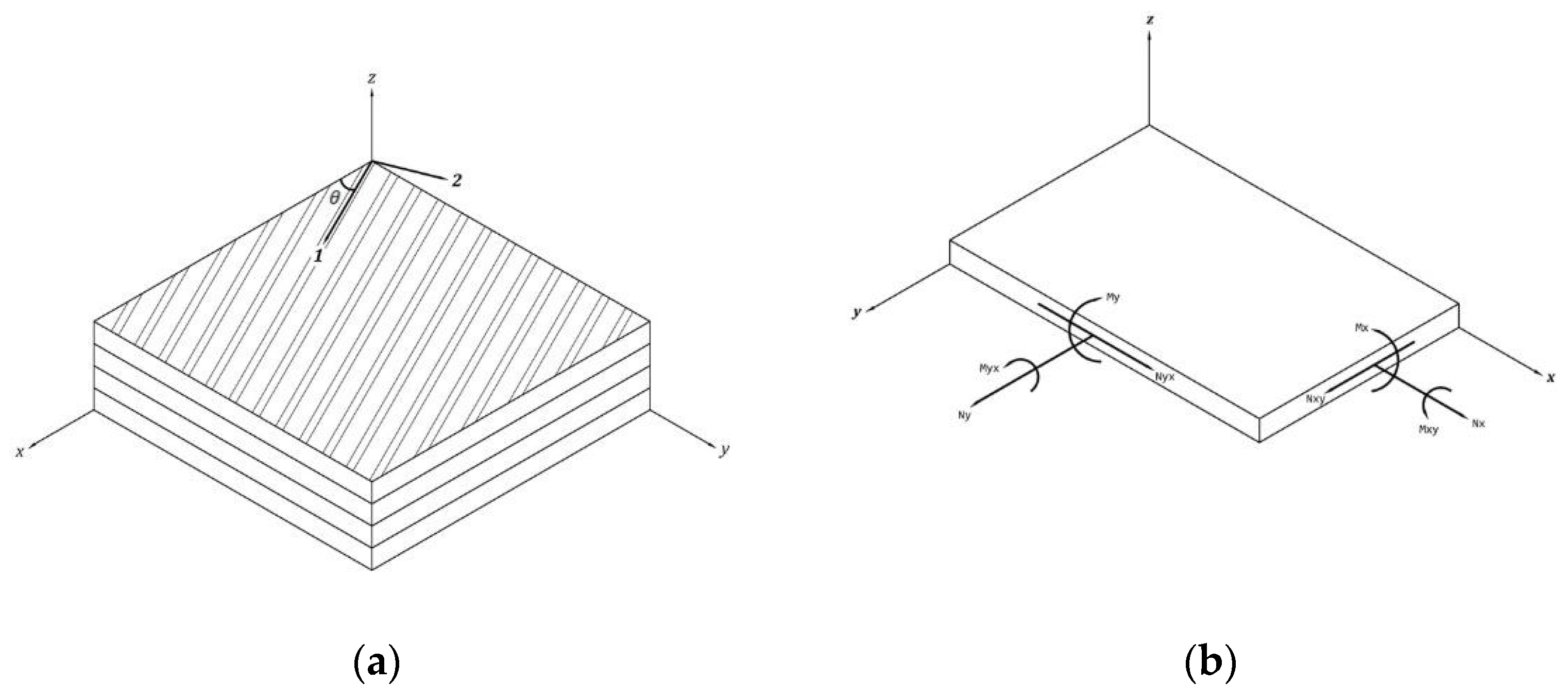
Figure 2.
Objective function values for GA and SA for study case 1.
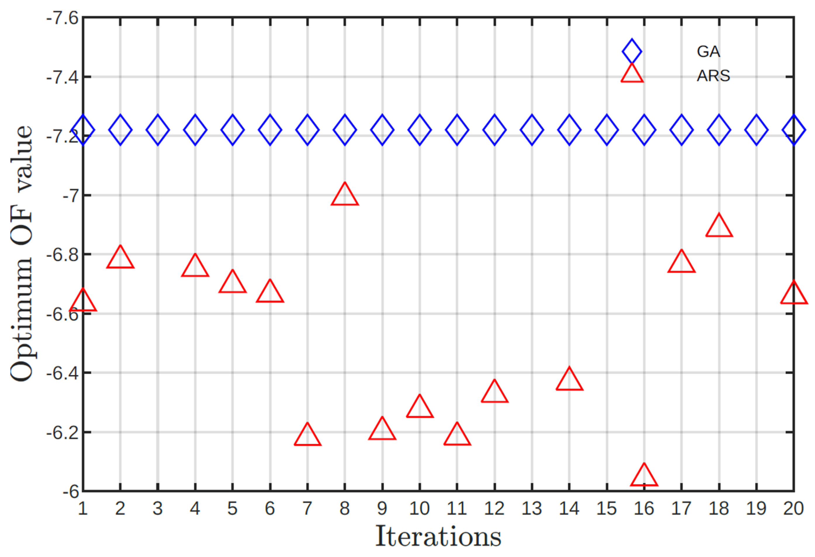
Figure 3.
Number of evaluations for GA and SA for study case 1.
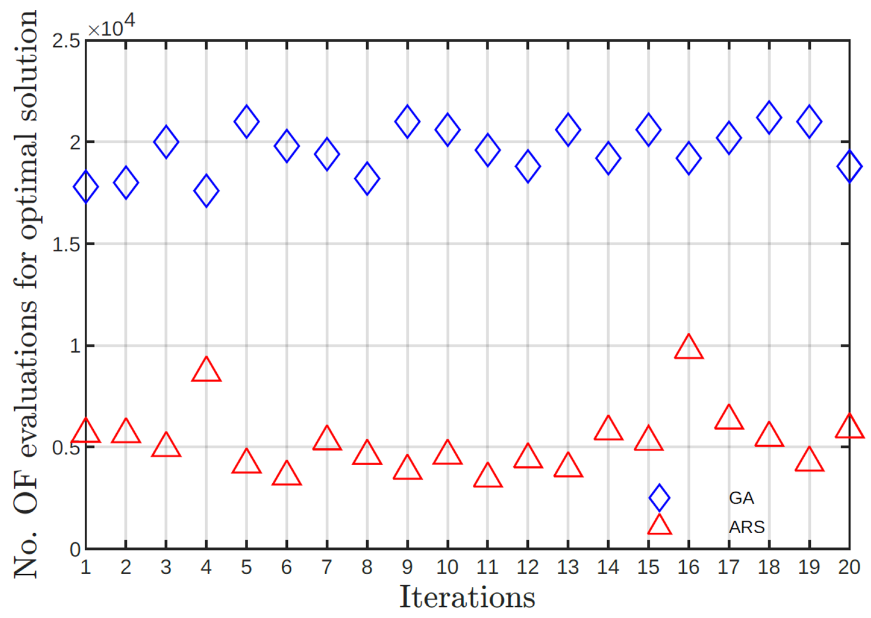
Figure 4.
Objective function values for GA and SA for study case 2.
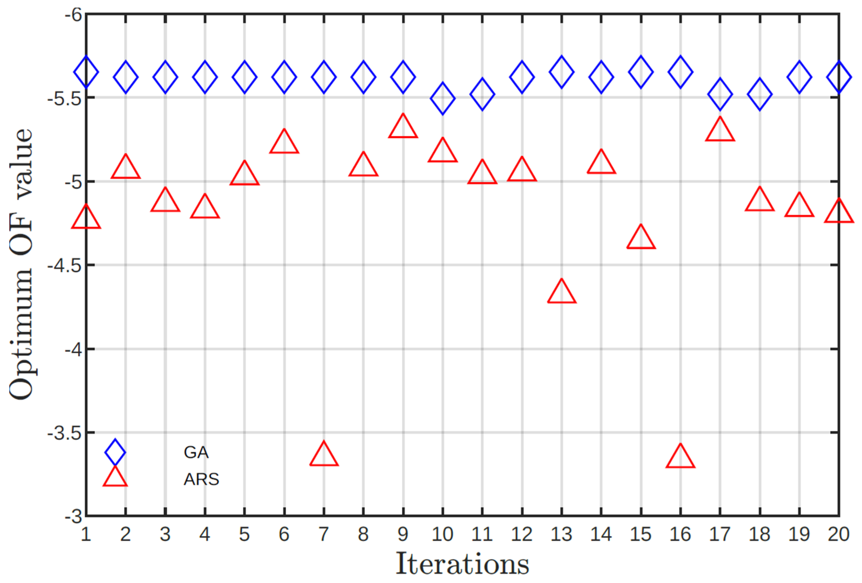
Figure 5.
Number of evaluations for GA and SA for study case 2.
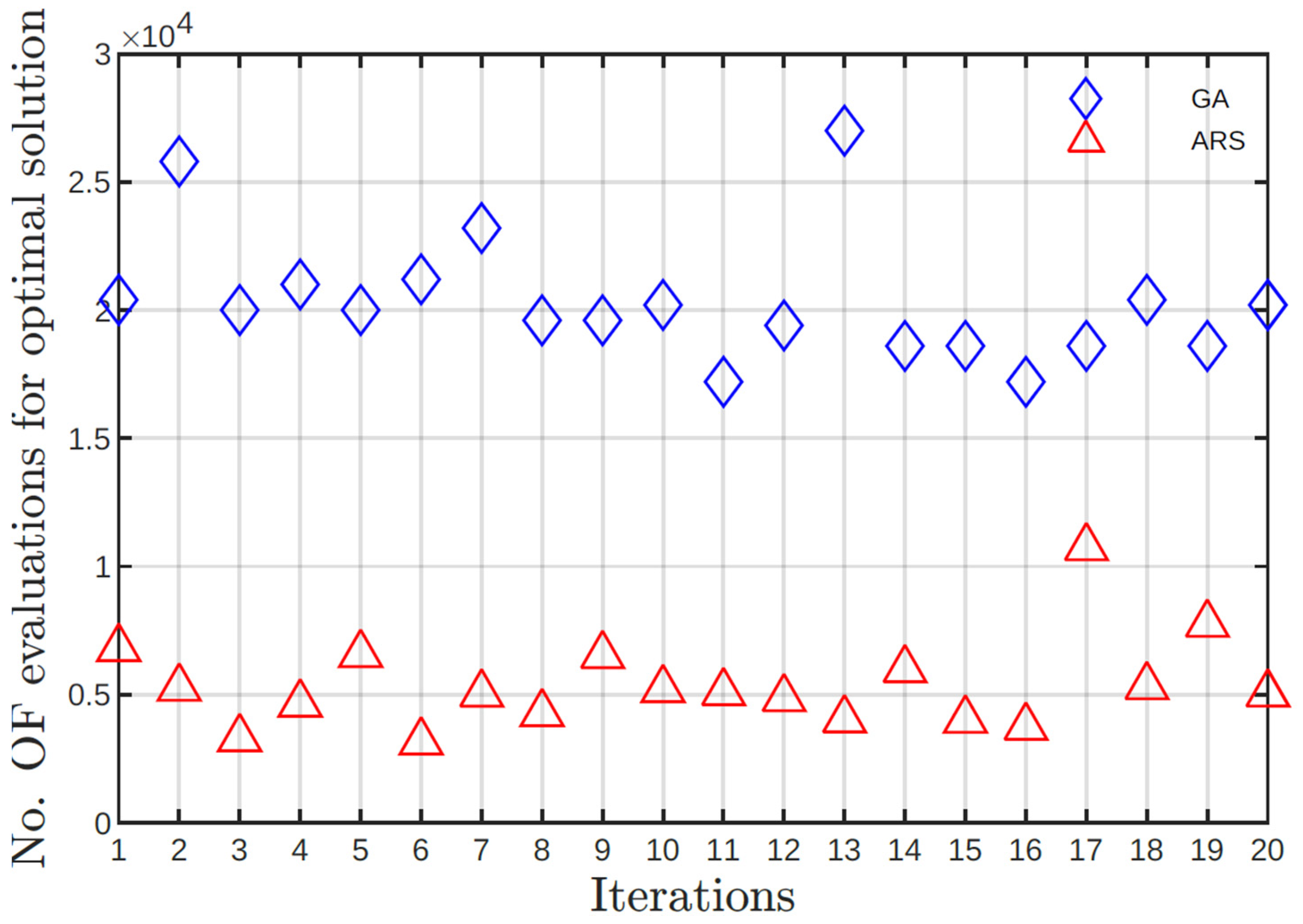

Table 1.
Orientation, SF and objective function for reference laminate, study case 1 - in-plane loads, Objective function = -3.5362.
Table 1.
Orientation, SF and objective function for reference laminate, study case 1 - in-plane loads, Objective function = -3.5362.
| Ply n |
Orientation (º) |
Safety Factor SF |
| 1 | 45 | 6.325 |
| 2 | -45 | 1.5755 |
| 3 | 0 | 2.7081 |
| 4 | 90 | 2.7081 |
| 5 | -45 | 1.5755 |
| 6 | 45 | 6.325 |
| 7 | 45 | 6.325 |
| 8 | -45 | 1.5755 |
| 9 | 90 | 2.7081 |
| 10 | 0 | 2.7081 |
| 11 | -45 | 1.5755 |
| 12 | 45 | 6.325 |
Table 2.
Orientation, SF and objective function for GA laminates best and worst solutions, study case 1 - in-plane loads, Objective function = -7.22.
Table 2.
Orientation, SF and objective function for GA laminates best and worst solutions, study case 1 - in-plane loads, Objective function = -7.22.
| Ply n |
Orientation (º) |
Safety Factor SF |
Orientation (º) |
Safety Factor SF |
| 1 | 45.00 | 9.588 | 135.02 | 2.483 |
| 2 | 134.99 | 2.483 | 44.99 | 9.588 |
| 3 | 45.00 | 9.588 | 135.01 | 2.483 |
| 4 | 134.99 | 2.483 | 45.01 | 9.588 |
| 5 | 45.00 | 9.588 | 44.98 | 9.588 |
| 6 | 44.99 | 9.588 | 44.98 | 9.588 |
| 7 | 44.99 | 9.588 | 44.98 | 9.588 |
| 8 | 45.00 | 9.588 | 44.98 | 9.588 |
| 9 | 134.99 | 2.483 | 45.01 | 9.588 |
| 10 | 45.00 | 9.588 | 135.01 | 2.483 |
| 11 | 134.99 | 2.483 | 44.99 | 9.588 |
| 12 | 45.00 | 9.588 | 135.02 | 2.483 |
Table 3.
Orientation, SF and objective function for SA laminates best and worst solution, study case 1 - in-plane loads, Objective function = -6.99 and -5.72.
Table 3.
Orientation, SF and objective function for SA laminates best and worst solution, study case 1 - in-plane loads, Objective function = -6.99 and -5.72.
| Ply n |
Orientation (º) |
Safety Factor SF |
Orientation (º) |
Safety Factor SF |
| 1 | 53.40 | 9.017 | 36.07 | 8.00 |
| 2 | 133.61 | 2.440 | 42.57 | 8.154 |
| 3 | 46.08 | 9.398 | 131.42 | 2.1477 |
| 4 | 40.57 | 9.282 | 69.23 | 5.564 |
| 5 | 42.98 | 9.375 | 40.50 | 8.152 |
| 6 | 131.86 | 2.446 | 149.02 | 2.337 |
| 7 | 131.86 | 2.446 | 149.02 | 2.337 |
| 8 | 42.98 | 42.98 | 40.50 | 8.152 |
| 9 | 40.57 | 9.282 | 69.23 | 5.564 |
| 10 | 46.08 | 9.398 | 131.42 | 2.1477 |
| 11 | 133.61 | 2.440 | 42.57 | 8.154 |
| 12 | 53.40 | 9.017 | 36.07 | 8.00 |
Table 4.
Orientation, SF and objective function for reference laminate, study case 2 - combined moments, Objective function = -2.5667.
Table 4.
Orientation, SF and objective function for reference laminate, study case 2 - combined moments, Objective function = -2.5667.
| Ply n |
Orientation (º) |
Safety Factor SF |
| 1 | -45 | 2.6089 |
| 2 | 45 | 1.3498 |
| 3 | 45 | 1.6873 |
| 4 | -45 | 5.2177 |
| 5 | 0 | 5.2362 |
| 6 | 90 | 9.8878 |
| 7 | 90 | 7.7220 |
| 8 | 0 | 3.5270 |
| 9 | -45 | 1.4479 |
| 10 | 45 | 4.4264 |
| 11 | 45 | 3.5411 |
| 12 | -45 | 0.7240 |
Table 5.
Orientation, SF and objective function for GA laminates best and worst solutions, study case 2 - combined moments, Objective function = -5.6533 and -5.4950.
Table 5.
Orientation, SF and objective function for GA laminates best and worst solutions, study case 2 - combined moments, Objective function = -5.6533 and -5.4950.
| Ply n |
Orientation (º) |
Safety Factor SF |
Orientation (º) |
Safety Factor SF |
| 1 | 44.99 | 1.171 | 45.003 | 1.081 |
| 2 | 135.00 | 3.898 | 135.00 | 4.054 |
| 3 | 45.00 | 1.757 | 44.98 | 1.622 |
| 4 | 135.00 | 6.497 | 45.00 | 2.162 |
| 5 | 45.00 | 3.515 | 3.515 | 3.244 |
| 6 | 44.99 | 7.039 | 135.00 | 20.274 |
| 7 | 44.99 | 21.430 | 135.00 | 5.741 |
| 8 | 45.00 | 10.715 | 44.99 | 10.644 |
| 9 | 135.00 | 1.808 | 45.00 | 7.096 |
| 10 | 45.00 | 5.3576 | 44.985 | 5.322 |
| 11 | 135.00 | 1.084 | 135.00 | 1.1484 |
| 12 | 44.99 | 3.571 | 45.00 | 3.548 |
Table 6.
Orientation, SF and objective function for SA laminates best and worst solutions, study case 2 - combined moments, Objective function = -5.3112 y -3.3396.
Table 6.
Orientation, SF and objective function for SA laminates best and worst solutions, study case 2 - combined moments, Objective function = -5.3112 y -3.3396.
| Ply n |
Orientation (º) |
Safety Factor SF |
Orientation (º) |
Safety Factor SF |
| 1 | 47.24 | 1.172 | 42.94 | 0.926 |
| 2 | 130.98 | 3.729 | 42.66 | 1.112 |
| 3 | 42.15 | 1.763 | 156.99 | 3.787 |
| 4 | 132.08 | 6.235 | 126.16 | 5.865 |
| 5 | 140.88 | 9.309 | 124.28 | 8.638 |
| 6 | 51.75 | 7.098 | 164.76 | 13.118 |
| 7 | 51.75 | 7.098 | 164.76 | 6.677 |
| 8 | 140.88 | 2.627 | 124.28 | 2.753 |
| 9 | 132.08 | 1.744 | 126.16 | 1.814 |
| 10 | 42.15 | 5.173 | 156.99 | 1.500 |
| 11 | 130.98 | 1.049 | 42.66 | 3.727 |
| 12 | 47.24 | 3.472 | 42.94 | 3.109 |
Table 7.
Orientation, SF and objective function for reference laminate, study case 3 - in-plane loads and combined moments, Objective function = -0.2888.
Table 7.
Orientation, SF and objective function for reference laminate, study case 3 - in-plane loads and combined moments, Objective function = -0.2888.
| Ply n |
Orientation (º) |
Safety Factor SF |
| 1 | 0 | 1.1144 |
| 2 | 45 | 1.1020 |
| 3 | -45 | 3.9891 |
| 4 | 45 | 1.5890 |
| 5 | 0 | 2.4426 |
| 6 | 90 | 1.4098 |
| 7 | 90 | 1.1437 |
| 8 | 0 | 2.2618 |
| 9 | 45 | 2.0125 |
| 10 | -45 | 0.6940 |
| 11 | 45 | 1.6355 |
| 12 | 0 | 1.3632 |
Table 8.
Orientation, SF and objective function for GA laminates best and worst solutions, study case 3 - combined moments, Objective function = -2.1946 and -1.9319.
Table 8.
Orientation, SF and objective function for GA laminates best and worst solutions, study case 3 - combined moments, Objective function = -2.1946 and -1.9319.
| Ply n |
Orientation (º) |
Safety Factor SF |
Orientation (º) |
Safety Factor SF |
| 1 | 21.66 | 1.501 | 22.60 | 1.218 |
| 2 | 24.38 | 1.647 | 24.38 | 1.346 |
| 3 | 145.30 | 5.036 | 27.00 | 1.497 |
| 4 | 139.03 | 3.558 | 37.46 | 1.638 |
| 5 | 44.34 | 1.942 | 129.87 | 2.229 |
| 6 | 48.61 | 1.977 | 130.12 | 1.828 |
| 7 | 48.61 | 2.008 | 130.12 | 1.529 |
| 8 | 44.34 | 2.110 | 129.87 | 1.303 |
| 9 | 139.03 | 1.070 | 37.46 | 2.438 |
| 10 | 145.30 | 1.000 | 27.00 | 2.774 |
| 11 | 24.38 | 2.325 | 24.62 | 2.738 |
| 12 | 21.66 | 2.156 | 22.60 | 2.639 |
Table 9.
Orientation, SF and objective function for SA laminates best and worst solution, study case 3 - combined moments, Objective function = -1.9461 and -0.8181.
Table 9.
Orientation, SF and objective function for SA laminates best and worst solution, study case 3 - combined moments, Objective function = -1.9461 and -0.8181.
| Ply n |
Orientation (º) |
Safety Factor SF |
Orientation (º) |
Safety Factor SF |
| 1 | 22.81 | 1.329 | 29.83 | 1.114 |
| 2 | 22.50 | 1.467 | 179.71 | 1.692 |
| 3 | 139.03 | 4.672 | 30.60 | 1.448 |
| 4 | 27.37 | 1.675 | 123.48 | 2.856 |
| 5 | 102.36 | 1.821 | 169.44 | 2.320 |
| 6 | 32.41 | 1.879 | 64.23 | 2.083 |
| 7 | 32.41 | 2.005 | 64.23 | 1.998 |
| 8 | 102.36 | 1.168 | 169.44 | 1.684 |
| 9 | 27.37 | 2.235 | 123.48 | 0.934 |
| 10 | 139.03 | 1.001 | 30.60 | 2.659 |
| 11 | 22.50 | 2.100 | 179.71 | 1.518 |
| 12 | 22.81 | 1.996 | 29.83 | 2.350 |
Disclaimer/Publisher’s Note: The statements, opinions and data contained in all publications are solely those of the individual author(s) and contributor(s) and not of MDPI and/or the editor(s). MDPI and/or the editor(s) disclaim responsibility for any injury to people or property resulting from any ideas, methods, instructions or products referred to in the content. |
© 2023 by the authors. Licensee MDPI, Basel, Switzerland. This article is an open access article distributed under the terms and conditions of the Creative Commons Attribution (CC BY) license (http://creativecommons.org/licenses/by/4.0/).
Copyright: This open access article is published under a Creative Commons CC BY 4.0 license, which permit the free download, distribution, and reuse, provided that the author and preprint are cited in any reuse.


