
Submitted:
21 September 2023
Posted:
22 September 2023
You are already at the latest version
Abstract
In this paper, we concentrate on the study of the properties of residual Tsallis entropy for
order statistics. Order statistics have an important role in reliability structural engineering
for example for modelling lifetimes of series and parallel systems. The residual Tsallis entropy
of ith order statistic from a continuous distribution function and its deviation from the
residual Tsallis entropy of ith order statistics from a uniform distribution is investigated. In
a mathematical framework, a method to express the residual Tsallis entropy of the ith order
statistic from a continuous distribution in terms of the residual Tsallis entropy of the ith
order statistic from a uniform distribution is provided. This approach may provide insight
into the behavior and properties of the residual Tsallis entropy for order statistics. Further,
we study the monotonicity properties of the residual Tsallis entropy of order statistics under
di
erent conditions. By studying these properties, deeper understanding of the relationship
between the position of order statistics and the resulting residual Tsallis entropy is gained.
Keywords:
order statistics
; residual Tsallis entropy
; Shannon entropy
; residual lifetime
; (n-i+1)-out-of-n system
1. Introduction
Information theory plays a crucial role in quantifying the uncertainty inherent in random phenomena. Its applications span a variety of areas, as detailed in Shannon’s influential work [1]. Considering a non-negative random variable X with an absolutely continuous cumulative distribution function (cdf) and a probability density function (pdf) , the Tsallis entropy of order becomes a relevant measure as defined in [2], given by
for all where denotes the expectation and for denotes the quantile function. In general, the Tsallis entropy can take negative values, but it can be made non-negative by choosing appropriate values of . An important observation is that , which illustrates the convergence of Tsallis entropy to Shannon differential entropy. Unlike the Shannon entropy, which exhibits additivity, the Tsallis entropy exhibits non-additivity. In particular, for two independent random variables X and Y in the Shannon framework holds, while in the Tsallis framework we find . The non-additive nature of the Tsallis entropy provides greater flexibility compared to the Shannon entropy, making it applicable in various areas of information theory, physics, chemistry, and technology.
Considering the lifetime of a newly introduced system denoted by X, the tsallis entropy serves as a measure of the inherent uncertainty of the system. However, there are cases where the actors have knowledge about the current age of the system. For example, they know that the system is operational at time t and want to evaluate the uncertainty in the remaining lifetime given by . In such scenarios, the conventional Tsallis entropy no longer provides the desired insight. Therefore, a new measure, the residual Tsallis entropy (RTE), is introduced, defined as follows:
where
is the pdf of and is the survival function of X.
Extensive research has been done in the literature to explore various properties and statistical applications of Tsallis entropy. For detailed insights, we recommend the work of Asadi et al. [3], Nanda and Paul [4], Zhang [5], Maasoumi [6], Abe [7], Asadi et al. [8], and the references cited in these works. These sources provide comprehensive discussions on this topic and allow for a deeper understanding of Tsallis entropy in various contexts.
The aim of this paper is to study the properties of RTE in terms of order statistics. We consider a random sample of size n from a distribution F denoted by . The order statistic represents the ordering of these sample values from smallest to largest, denoted . Order statistics are very important in many areas of probability and statistics because they can be used to describe probability distributions, to test how well a data set fits a particular model, to control the quality of a product or process, to analyze the reliability of a system or component, and for many other applications.
Moreover, they are indispensable in reliability theory, especially for studying the lifetime properties of coherent systems and performing lifetime tests on data obtained by various censoring methods. For a thorough understanding of the theory and applications of order statistics, we recommend the comprehensive review by David and Nagaraja [9]. This source covers the topic in depth and provides useful insights into the theoretical and practical aspects of order statistics. Many researchers have studied the information properties of order statistics and have gained useful insights, which can be found in [10,11,12] and the references therein. Zarezadeh and Asadi [13] studied properties of residual Renyi entropy of order statistics and record values; see also [14]. Continuing this line of research, our study aims to contribute to the field by investigating the properties of residual Tsallis entropy in terms of order statistics. More recently, Alomani and Kayid [15] have studied the properties of the Tsallis entropy of a coherent and mixed system.
The results of this work is structured as follows: In Section 2, we present the representation of RTE for order statistics denoted as from a sample drawn from an arbitrary continuous distribution function We express these RTE in terms of RTE for order statistics from a sample drawn from a uniform distribution. Since closed-form expressions for the RTE of order statistics are often not available for many statistical models, we derive upper and lower bounds to approximate the RTE. We provide several illustrative examples to demonstrate the practicality and usefulness of these bounds. In addition, we study the monotonicity properties of RTE for the extremum of a sample under mild conditions. We find that the RTEs of the extremum of a random sample exhibit monotonic behavior as the number of observations in the sample increases. However, we counter this observation by presenting a counterexample that demonstrates the non-monotonic behavior of RTE for other order statistics with respect to sample size. To further analyze the monotonic behavior, we examine the RTE of order statistics with respect to the index of order statistics Our results show that the RTE of is not a monotonic function of i over the entire support of
Throughout the paper, “" and “" stand for usual stochastic and likelihood ratio orders, respectively, for more details on these orderings, we refer the reader to Shaked and Shanthikumar [16].
2. Residual Tsallis Entropy of Order Statistics
Hereafter, we present an expression for the RTE of order statistics in relation to the RTE of order statistics from a uniform distribution. Let us consider the pdf and the survival function of denoted by and , respectively, where . It holds that
where
is known as the complete beta function; see e.g., David and Nagaraja [9]. Furthermore, we can express the survival function as follows:
where
is known as the incomplete beta functions. In this section, we adopt the notation to denote that the random variable Y follows a truncated beta distribution with pdf given by:
The paper is concerned with the study of the residual tsallis entropy of the random variable , which measures the degree of uncertainty about the predictability of the residual lifetime of the system contained in the density of . In reliability engineering, -out-of-n systems are an important type of structure. In this case, an -out-of-n system functions if and only if at least components of n components function. We consider a system consisting of independent and identically distributed components whose lifetimes are represented by . The lifetime of the whole system is determined by the order statistic , where i denotes the position of the order statistic. When , this corresponds to a serial system, while represents a parallel system. In the context of -out-of-n systems operating at time t, the RTE of serves as a measure of entropy associated with the remaining lifetime of the system. This dynamic entropy measure provides system designers with valuable information about the entropy of -out-of-n systems in operation at a given time t.
To increase computational efficiency, we introduce a lemma that establishes a relationship between the RTE of order statistics from a uniform distribution and the incomplete beta function. This relation is crucial from a practical point of view and allows for a more convenient computation of RTE. The proof of this lemma, which follows directly from the definition of RTE, is omitted here because it involves simple computations.
Lemma 1.
Suppose we have a random sample of size n from a uniform distribution on (0,1) and we arrange the sample values in ascending order where the i-th order statistic. Then
for all
Using this lemma, researchers and practitioners can easily compute the RTE of order statistics from a uniform distribution using the well-known incomplete beta function. This computational simplification improves the applicability and usability of RTE in various contexts. In Figure 1, we show the plot of for different values of and when the total number of observations is . The figure shows that there is no inherent monotonicity between the order statistics. However, in the following analysis (Lemma 3), we establish conditions under which a monotonic relationship can be established between the index i and the number of components in the system. This lemma will provide valuable insight into the arrangement of the system components and the resulting effect on the reliability of the system.
The upcoming theorem establishes a relationship between the RTE of order statistics and the RTE of order statistics from a uniform distribution.
Theorem 1.
The residual Tsallis entropy of for all can be expressed as follows:
where
Proof.
After some calculation, it can be seen that when in (7) the order goes to unity, the Shannon entropy of i-th order statistic from a sample of F can be written as follows:
where The specialized version of this result for was already obtained by Ebrahimi et al. [12]. Below, we provide an example for illustration.
Example 1.
Suppose that X is a standard exponential distribution with mean unity. Then and we have
Thus, from (7), we obtain
In Figure 2, we plotted for some values of and when When , we can use (10) to get
Also, we know that
Therefore, we have
This finding reveals an intriguing characteristic: the discrepancy between the RTE of the lifetime of a series system and the RTE of each component is not influenced by time. Instead, it solely relies on two factors: the number of components within the system and the parameter in the exponential case.
While we have successfully obtained a closed expression for the first order statistics of RTE in the exponential distribution, the task becomes significantly more difficult when we consider the higher order statistics in some other distributions. Unfortunately, closed-form expressions for the RTE of higher-order statistics in these distributions, as well as in many other distributions, are generally not available. Given this limitation, we are motivated to explore alternative approaches to characterizing the RTE of order statistics. We therefore propose to establish thresholds for the RTE of order statistics. To this end, we present the following theorem as a conclusive proof that provides valuable insight into the nature of these bounds and their applicability in practical scenarios.
Theorem 2.
Consider a non-negative continuous random variable X with pdf f and cdf Let us denote the RTEs of X and the i-th order statistic as and respectively.
- (a)
- Let where is the mode of the distribution of , then for we have
- (b)
- Suppose we have where m is the mode of the pdf f, such that . Then, for any we obtain
Proof.
(a) By applying Theorem 2.3, we only need to find a bound for To this aim, for we have
The result now is easily obtained by recalling (7).
(b) Since for it holds that
one can write
The result now is easily obtained from relation (7) and this completes the proof. □
The given theorem branches into two elements. The first subdivision, denoted (i), establishes a lower bound for the RTE associated with , denoted . It should be noted that the given lower bound can be transformed into an upper bound under certain conditions. This bound is formed by using the incomplete beta function together with the RTE of the original distribution. Conversely, in part (ii) of the theorem, a lower bound is introduced for the RTE of , denoted as . This lower bound is expressed via the RTE of order statistics from a uniform distribution and the mode, represented by m, of the underlying distribution. This finding provides interesting insights into the information properties of and provides a quantifiable measure of the lower bound of RTE with respect to the mode of the distribution.
In the following lemma we deal with the monotonic behavior of the RTE of order statistics. To lay the groundwork for our subsequent findings, we first introduce a central lemma that plays a fundamental role in our analysis.
Lemma 2.
Consider two non-negative functions, and , where is an increasing function. Let t and c be real numbers such that . Additionally, assume that the random variable follows a pdf , where as
Let r be real valued and define function as follows:
- (i)
- If for then is an increasing function of
- (ii)
- If for then is a decreasing function of
Proof.
We just prove Part (i) since the proof for Part (ii) is similar. Assuming that is differentiable in terms of r, we can obtain
where
It is evident that
Using the fact that and that is an increasing function, one can show that . This implies that (13) is non-positive (non-negative), and hence is an increasing function of r. □
Corollary 1.
Under the assumptions of Lemma 2, it can be proven that when is decreasing, the following holds:
- (i)
- For then is a decreasing function of
- (ii)
- If for then is a increasing function of
Due to Lemma 2, we can prove the following corollary for -out-of-n systems with components having uniform distributions.
Lemma 3.
- (i)
- When considering a parallel (series) system consisting of n components with a uniform distribution over the unit interval, the RTE of the system lifetime decreases as the number of components increases.
- (ii)
- If are integers, then for
Proof.
(i) The presumption is that the system operates in parallel. Analogous reasoning can be applied to a series system to authenticate the outcome via Remark 2.9. From Lemma 1, we get
So, Lemma 2 readily reveals that can be depicted as (12) where and . We adopt the assumption, devoid of any generality loss, that is a continuous variable. Considering the ratio
is increasing (decreasing) in t and hence we can establish the inequality
where the pdf of is defined in equation (11). By applying Lemma 2, we can deduce that the RTE of the parallel system is a decreasing function as the number of components increases.
(ii) To begin, we observe that
Furthermore, the pdf of as stated in (11) is expressed as
where in this context and Hence, it is apparent that for and (or ), we can write
In conclusion, it can be inferred for that
and this signifies the end of the proof. □
Theorem 3.
Consider a parallel (series) system consisting of n independent and identically distributed random variables representing the lifetime of the components. Assume that the common distribution function F has a pdf f that is increasing (decreasing) in its support. Then, the RTE of the system lifetime is decreasing in
Proof.
Assuming that then indicates the pdf of It is evident that
is increasing in This implies that and therefore . Moreover, for is an increasing (decreasing) function of Therefore
From Theorem 2.3, for we have
The first inequality is obtained by noting that is non-negative. The last inequality is obtained from Part (i) of Lemma 3. Thus, one can conclude that for all □
Many distributions have decreasing pdfs, such as the exponential distribution, the Pareto distribution, and mixtures of these two. On the other hand, some distributions have increasing pdfs, such as the power distribution with its density function. Using part (i) of the corollary 1, we can prove a theorem for distributions whose pdfs go up or down. But we have to be careful, because this theorem does not work for all kinds of -out-of-n systems, as the next example shows.
Example 2.
Let us consider the system works if at least of its n components work. Then, the system’s lifetime is the second smallest component lifetime, The components have the same distribution, uniform on In Figure 3, we see how the RTE of changes with n when and The graph shows that the RTE of the system does not always decrease as n increases. For example, it reveals that is less than that of .
In reliability theory, we can imagine a case where the pdf decreases, and thus the RRE of a serial system decreases, when the system has more components. This happens when we have a lifetime model with a failure rate () that decreases with time. Then the data distribution must have a density function that also decreases. Some lifetime distributions in the reliability domain have the property that their RTE decreases as their scale parameter increases. This is the case, for example, with the Weibull distribution with a shape parameter less than one and with the Gamma distribution with a shape parameter less than one. Therefore, the RTE of a series system with components following these distributions becomes smaller as the number of components increases.
Now, we want to see how the RTE of order statistics changes with We use Part (ii) of Lemma 3, which gives us a formula for the RTE of in terms of
Theorem 4.
Suppose X is a continuous random variable that is always positive. Its distribution function is F and its pdf is The pdf f decreases over the range of possible values of Let and be two whole numbers such that Then the RTE of the -th smallest value of X among n samples, is less than or equal to the RTE of the -th smallest value, for all values of X that are greater than or equal to the th percentile of
Proof.
For it is easy to verify that and hence . Now, we have
Using Part (ii) of Lemma 3 and the same reasoning as in the proof of Theorem 3, we can obtain the result. □
The following example shows that the condition cannot be dropped from the conditions of theorem.
Example 3.
Assume the survival function of X as
In Figure 4, we see how the RTE of order statistics for and , changes with The plots show that the RTE of the order statistics does not always go up or down as i goes up for all values of For example, for the values of the RTE is not monotonic in terms of
We can get a useful result from Theorem 4.
Corollary 2.
Suppose X is a non-negative continuous random variable that is always positive with cdf F and pdf The pdf f decreases over the range of possible values of Let i be a whole number that is less than or equal to half of Then, the RTE of is increasing in i for values of t greater than the median of distribution.
Proof.
Suppose This means that
where is the middle value of By Theorem 4, we get for that □
3. Conclusion
This article addresses the concept of RTE for order statistics. We have presented a new approach to express the RTE of order statistics from a continuous distribution in terms of the RTE of order statistics from a uniform distribution. This connection provides valuable insight into the properties and behavior of RTE for different distributions. Furthermore, due to the complexity of obtaining closed-form expressions for RTE of order statistics, we have derived bounds that provide practical approximations and allow a better understanding of their properties. These bounds serve as useful tools for analyzing and comparing RTE values in different scenarios. In addition, we examined the influence of the index of order statistics, denoted i, and the total number of observations, denoted n, on RTE. By examining the changes in RTE with respect to i and n, we gained a deeper understanding of the relationship between the position of the order statistic and the entropy of the overall distribution. To validate our results and demonstrate the applicability of our approach, we have provided illustrative examples. These examples demonstrate the practical implications of RTE for order statistics and illustrate the versatility of our methodology for different distributions. In summary, this study contributes to the understanding of RTE for order statistics by establishing relationships, deriving bounds, and investigating the influence of index and sample size. The results of this work provide valuable insights for researchers and practitioners working in the field of statistical inference and entropy-based analysis.
Acknowledgments
The authors acknowledge financial support from the Researchers Supporting Project number (RSP2023R464), King Saud University, Riyadh, Saudi Arabia.
References
- Shannon, C.E. A mathematical theory of communication. The Bell system technical journal 1948, 27, 379–423. [Google Scholar] [CrossRef]
- Tsallis, C. Possible generalization of Boltzmann-Gibbs statistics. Journal of statistical physics 1988, 52, 479–487. [Google Scholar] [CrossRef]
- Asadi, M.; Ebrahimi, N.; Soofi, E.S. Dynamic generalized information measures. Statistics & probability letters 2005, 71, 85–98. [Google Scholar] [CrossRef]
- Nanda, A.K.; Paul, P. Some results on generalized residual entropy. Information Sciences 2006, 176, 27–47. [Google Scholar] [CrossRef]
- Zhang, Z. Uniform estimates on the Tsallis entropies. Letters in Mathematical Physics 2007, 80, 171–181. [Google Scholar] [CrossRef]
- Maasoumi, E. The measurement and decomposition of multi-dimensional inequality. Econometrica: Journal of the Econometric Society 1986, 991–997. [Google Scholar] [CrossRef]
- Abe, S. Axioms and uniqueness theorem for Tsallis entropy. Physics Letters A 2000, 271, 74–79. [Google Scholar] [CrossRef]
- Asadi, M.; Ebrahimi, N.; Soofi, E.S. Connections of Gini, Fisher, and Shannon by Bayes risk under proportional hazards. Journal of Applied Probability 2017, 54, 1027–1050. [Google Scholar] [CrossRef]
- David, H.A.; Nagaraja, H.N. Order statistics; John Wiley & Sons, 2004. [Google Scholar]
- Wong, K.M.; Chen, S. The entropy of ordered sequences and order statistics. IEEE Transactions on Information Theory 1990, 36, 276–284. [Google Scholar] [CrossRef]
- Park, S. The entropy of consecutive order statistics. IEEE Trans. Inf. Theory 1995, 41, 2003–2007. [Google Scholar] [CrossRef]
- Ebrahimi, N.; Soofi, E.S.; Soyer, R. Information measures in perspective. Int. Stat. Rev. 2010, 78, 383–412. [Google Scholar] [CrossRef]
- Zarezadeh, S.; Asadi, M. Results on residual Rényi entropy of order statistics and record values. Information Sciences 2010, 180, 4195–4206. [Google Scholar] [CrossRef]
- Baratpour, S.; Ahmadi, J.; Arghami, N.R. Characterizations based on Rényi entropy of order statistics and record values. Journal of Statistical Planning and Inference 2008, 138, 2544–2551. [Google Scholar] [CrossRef]
- Alomani, G.; Kayid, M. Further Properties of Tsallis Entropy and Its Application. Entropy 2023, 25, 199. [Google Scholar] [CrossRef] [PubMed]
- Shaked, M.; Shanthikumar, J.G. Stochastic orders; Springer Science & Business Media, 2007. [Google Scholar]
Figure 1.
The exact values of for (left panel) and (right panel) with respect to
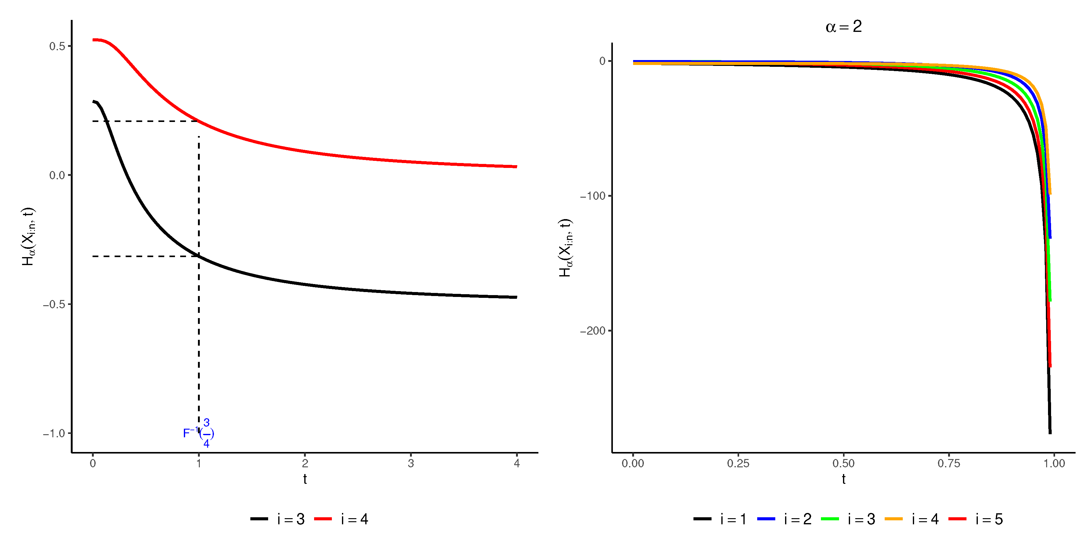
Figure 2.
The exact values of for (left panel) and (right panel) with respect to
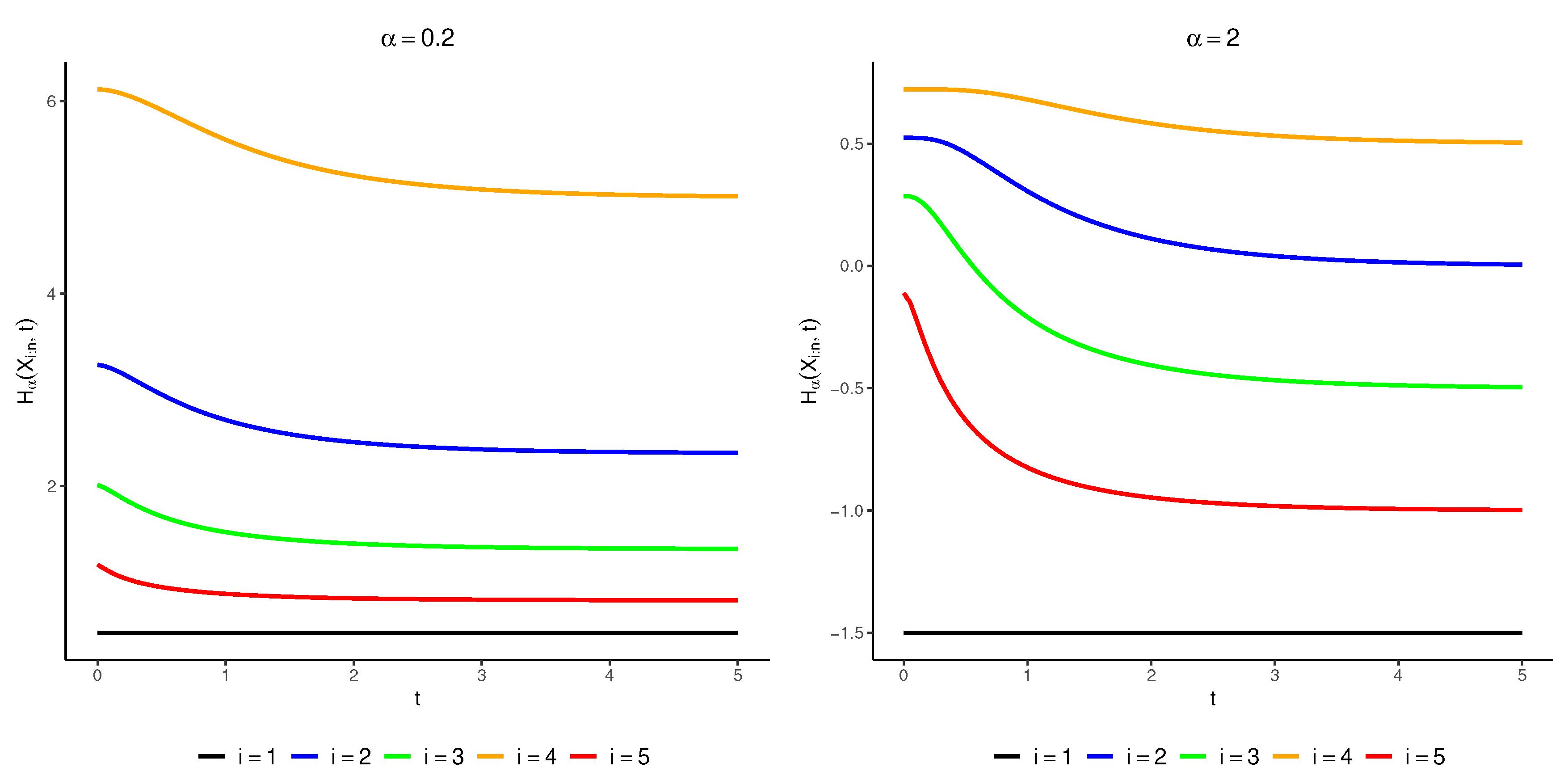
Figure 3.
The RTE values for different n in a -out-of-n system with a uniform parent distribution and when
Figure 3.
The RTE values for different n in a -out-of-n system with a uniform parent distribution and when
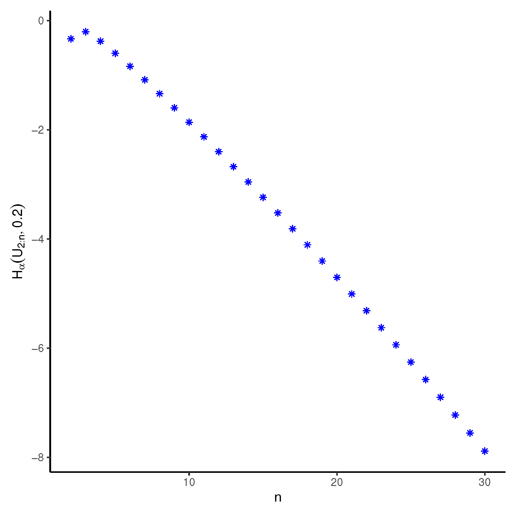
Figure 4.
The RTE values for different n in a -out-of-n system with a uniform parent distribution and when
Figure 4.
The RTE values for different n in a -out-of-n system with a uniform parent distribution and when
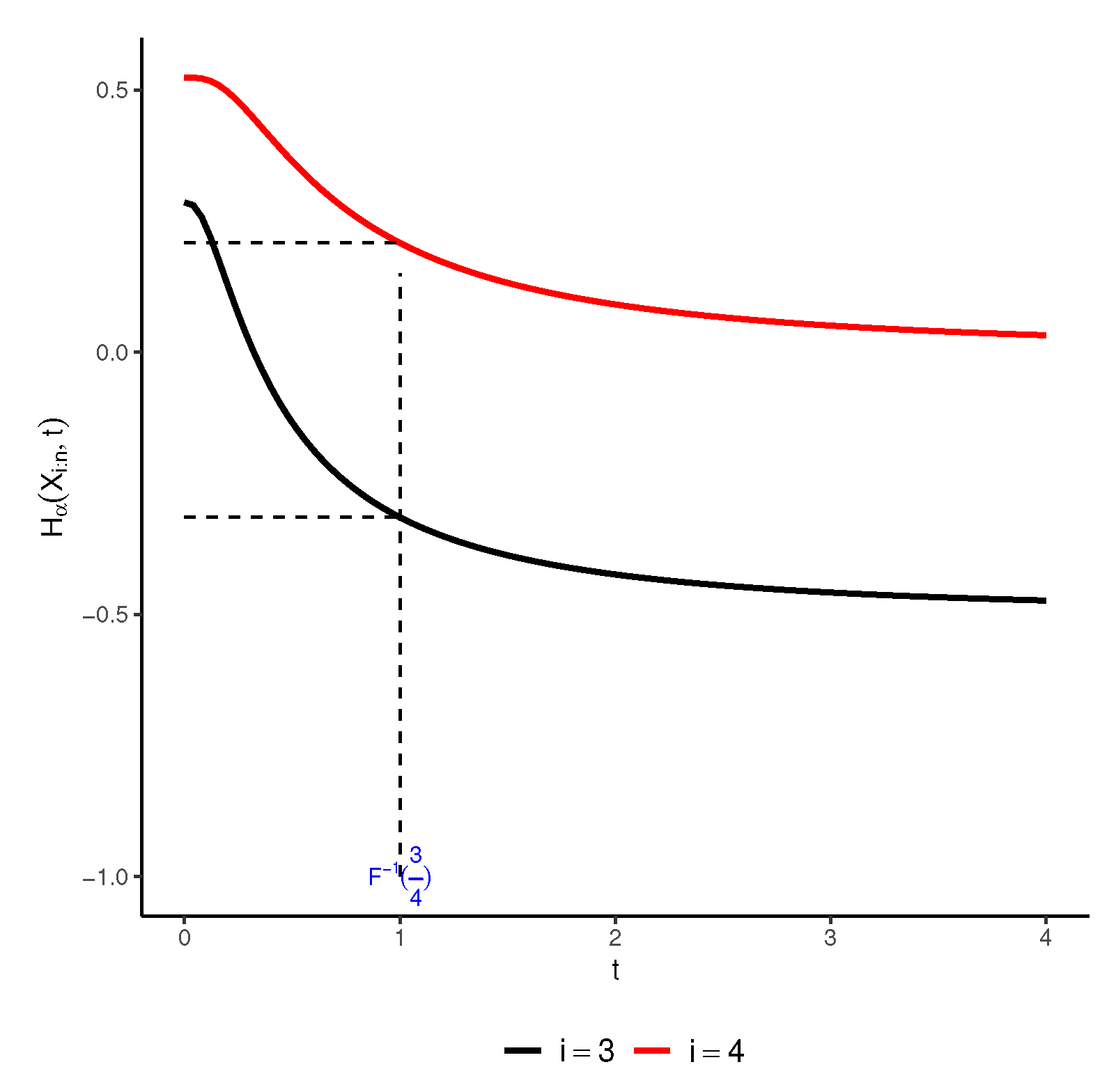

Table 1.
Bounds on derived from Theorem 2 (Parts (i) and (ii)).
| Probability Density Function | Bounds | |
Disclaimer/Publisher’s Note: The statements, opinions and data contained in all publications are solely those of the individual author(s) and contributor(s) and not of MDPI and/or the editor(s). MDPI and/or the editor(s) disclaim responsibility for any injury to people or property resulting from any ideas, methods, instructions or products referred to in the content. |
© 2023 by the authors. Licensee MDPI, Basel, Switzerland. This article is an open access article distributed under the terms and conditions of the Creative Commons Attribution (CC BY) license (http://creativecommons.org/licenses/by/4.0/).
Copyright: This open access article is published under a Creative Commons CC BY 4.0 license, which permit the free download, distribution, and reuse, provided that the author and preprint are cited in any reuse.


