
Submitted:
19 September 2023
Posted:
20 September 2023
You are already at the latest version
Abstract
Facial emotion detection is a challenging task that deals with emotion recognition. It has applications in various domains, such as behavior analysis, surveillance systems and human-computer interaction (HCI). Numerous studies have been implemented to detect emotions, including classical machine learning algorithms and advanced deep learning algorithms. For the machine learning algorithm, the hand-crafted feature needs to be extracted, which is a tiring task and requires human effort. Whereas in deep learning models, automated feature extraction is employed from samples. Therefore, in this study, we have proposed a novel and efficient deep learning model based on Neural Architecture Search Network utilizing superior artificial networks such as RNN and child networks. We performed the training utilizing the FER 2013 dataset comprising seven classes: happy, angry, neutral, sad, surprise, fear, and disgust. Furthermore, we analyzed the robustness of the proposed model on CK+ datasets and comparing with existing techniques. Due to the implication of reinforcement learning in the network, most representative features are extracted from the sample network. It extracts all key features without losing the key information. Our proposed model is based on one stage classifier and performs efficient classification. Our technique outperformed the existing models attaining an accuracy of 98.14%, recall of 97.57%, and precision of 97.84%.
Keywords:
Facial Emotion Detection
; Deep Learning
; Classification
; Neural Architecture Search Network
1. Introduction
Emotions are an unavoidable way of communicating among individuals. They can be suppressed differently, which may not be unmistakable to bare eyes. There has been an increased need for humans to understand emotion recognition over the past few years, and it has numerous applications, such as computer interactions [1], animations, medication [2], safety [3], diagnosing Autism Spectrum Disorder (ASD) in children [4].
With the rapid growth of developments of machine learning and deep learning algorithms, numerous applications exist for analyzing human emotions, such as robot health care techniques and direct human-computer interactions [5,6,7]. Thus, our daily actions usually depend on the emotional expressions of others [8]. Therefore, the expressions can be evaluated considering various factors, such as face expression [9], speech [10], and electroencephalogram (EEG) [11]. The confront talks are among the most prevalent among these highlights for many reasons. They are effortlessly reasonable and contain numerous valuable emotions, and there are available databases to do experiments and introduce automated models for facial emotion recognition [12].
Figure 1 shows some samples of facial expressions from the three databases: FER, JAFFE, and FERG.
In machine learning-based models, the feature extraction process in FER is performed manually, which is time-consuming and involves human effort. Support Vector Machine (SVM) and decision tree algorithms have primarily been used for FER. However, it may be critical to extract the manual features from the various zones of a face, as in a single emotion, all parts of the face do not convey the information. This implies that a perfect algorithm using machine learning techniques should consider that the imperative part of the face is less sensitive than other facial regions. However, the deep learning-based techniques for FER involve automated feature extraction due to its layered architecture consisting of Pooling, Convolutional, and Fully Connected Layers [14]. Features are extracted continuously and are transferred to the classification layer for categorization. Hence, analyzing the significance of convolutional neural networks and DL methods, they have been utilized in facial expression recognition [15]. These deep learning-based models employ processing similar to human brains and compute the key points without human effort. As a result, deep learning models perform better than machine learning-based methods in most scenarios. With the advancement in hardware tools, deep learning architectures are explored extensively to solve classification problems in less time. Some of the deep learning models have performed very well for the FER, such as MBP [16], VGG [17], and the Fully connected layer [18]; however, there is still a need for improvements.
Deep learning-based models perform better for object localization and classification problems than machine learning-based models [19]. Although there have been various significant applications of machine learning-based methods, on the other side, they are based on complex codes. They are less efficient due to their ample processing time. Furthermore, deep learning-based methods are more generalized and can be used for similar problems. In contrast, machine learning-based solutions cannot be used for multiple region classification in a single input sample.
Moreover, deep learning-based techniques perform well. However, various challenges in FER systems still exist that should be considered and coped with using the latest techniques. These challenges include emotion analysis in occlusion videos, real-time FER [20], and addressing the uncontrolled environment, such as variations in facial angles, brightness, face texture, and so on [21,22]. Therefore, accurate and effective facial region localization and classification localization are still tricky tasks. Thus, this study proposes an efficient model based on a Neural Architecture Search Network based on a reinforcement learning block. Our proposed model is based on fundamental building blocks called cells, comprising various layers, such as convolutional, detailed convolutional, and depth-wise separable layers, which help effectively detect emotions.
2. Related Work
Bargshady et al. [17] developed a technique based on Bidirectional Long Short Term Memory (BiLSTM) for the 4 phases of pain recognition. The PCA algorithm has been employed for the dimensionality reduction of the features. The proposed algorithm achieved 98.4% area under the curve and 90% test precision using the UNBC-McMaster Shoulder Pain database. Chen et al. [23] proposed a two-stage technique based on DCNN to categorize facial expressions. The method was based on two phases: the SoftMax score calculation for binary CNN and the classification through DCNN. The proposed technique coped with the challenge of neutral language variations and achieved an accuracy of 96.28%. Zou et al. [24] developed the system for FER based on batch regularization and the ReLU activation function CNN to cope with the problem of the gradient disappearing. The dropout technique has been utilized to overcome the network fitting. They implemented the two algorithms, AlexNet and VGG-19; thus, the latter results are better. The average FER score was 6.9% higher than the AlexNet. Wang et al. [25] proposed a model based on features extracted from CNN and the C4.5 classifier to recognize facial expressions, preventing the void of hand-crafted features. They also proposed various changes in C4.5 and the traditional RF algorithm. Moreover, a Decision Tree (DT) has also been proposed for the classification. Therefore, based on the features, the RF algorithm has been used for the FER.
In [26], Wang et al. proposed a system based on LeNet-5 to cope with the challenges such as less knowledge of image and occlusion, reducing the accuracy of traditional machine learning. They employed a LeNet-5 classifier and computed the parameters such as learning rate, kernel size, and CNN excitation function. The model was stable and detected the facial expressions robustly under the occlusion. The algorithm attained 97.23% accuracy over the dataset CK. Additionally, Wang et al. [18] developed an approach using hybrid characteristics of two models such as CNN and Convolutional Restricted Boltzmann Machine (CRBM). They utilized the modified CRBM by replacing the fully connected layers of traditional CNN. The images have been classified effectively, employing efficient approaches.
Moreover, the variation in the sets of images did not affect the recognition performance. Fei et al. [27] developed a system for recognizing emotional intelligence based on deep CNN to recognize the mental diagnosis. Deep features have been extracted from images using an AlexNet 6 sheet with a linear LDA for the classification. The system is based on three main phases: input videos, images pre-processing, and prediction of expressions. The evaluation process exhibited that the proposed approach outperformed the existing techniques and proved to be a cheap method to diagnose the mental state using facial expressions. Ameur et al. [16] proposed a technique using Monogenic Binary Pattern (MBP) and CNN. First, the salient features were extracted using MBP, and then DCNN was employed to classify the expressions. The proposed algorithm attained significant performance while considering the challenges such as lighting, texture, facial forms, and occlusion.
Different strategies have been proposed for facial emotion analysis; some are based on machine learning techniques, while most include CNN or deep learning architecture. However, there is still a need to propose a robust system for facial recognition that overcomes all challenges, such as varieties in lighting, angle, camera, background, and occlusion. The existing models failed to cope with all these challenges simultaneously for the FER. Therefore, in the proposed study, we propose a robust model for the FER based on deep learning that overcomes all the problems above and performs facial emotion recognition effectively. The details of existing work are presented in Table 1.
3. Methodology
In this paperwork, we created a mobile application that employs deep learning for face emotion detection. In the first stage, we gather a dataset for training our proposed model based on the Neural Architecture Search Network. It employs cells as basic blocks utilizing reinforcement learning. Our proposed model is easy and fast to implement. The detailed steps are given below.
3.1. Datasets
First, we acquired the FER 2013 [38] comprising grayscale images of size 48x484 exhibiting faces. All the images have only faces that were less or more centered. The dataset consists of seven classes: happy, disgust, fear, neutral, sad, surprise and angry. We employed the FER 2013 dataset for the training of our proposed model. The training data has 28,610 samples and 7069 test samples.
Moreover, the Angry class has 3874 images, the Disgust class has 465 images, the Fear class has 4107 images, Happy class has 6998 images, the Neutral class has 5175 images, Sad class has 4790 images, and the Surprise class has 3201 images. However, the test dataset has distributed as follows: Angry class has 947 images, Disgust class has 123 images, the Fear class has 1134 images, Happy class has 1801 images, Neutral class has 1199 images, Sad class has 1109 images, and Surprise class has 756 images. Second, we employed the CK+ dataset, which is publicly available to validate our proposed model. The CK+ dataset has also been divided into seven classes representing emotions: angry, contempt neutral, fear, disgust, happy, surprise and sad. The size of the images was 256 x 256. The anger class samples were 135, contempt class samples were 54, disgust class samples were 177, fear class samples were 75, happy class samples were 207, sad class samples were 84, and surprise class samples were 249. Figure 2 shows sample database images, and Table 2 provides an overview of the dataset.
The entire database is divided into training and test sets by randomly dividing the images. We used 7069 images for testing and 28610 images for training, including different emotions: anger, disgust, fear, joy, neutral, sadness, and surprise. The 80/20 distribution is mainly used in neural network applications; other distributions (such as 70/30, 75/25) do not have a sufficient impact on the performance of the developed model. This study uses 28,610 images to train the Efficient Neural Architecture Search Network mobile model, and 7,069 are used to validate the model's performance for facial emotion recognition and classification.
3.2. Deep Learning-Based Classification
Classical machine learning systems require manual feature extraction, and then features are fed to the classifier for training. This process is doable for less complex problems. However, for more complex problems, such as emotion recognition, ML traditional techniques may fail and require additional effort. In contrast, the automatic feature extraction method allows deep learning models to excel. Figure 3 shows the difference between a traditional machine-learning style and a deep-learning approach. A deep learning approach is built on artificial intelligence networks (ANNs). In neural networks, which are based on layers of multiple neurons, communication is formed between neurons of adjacent layers. Although the deep traditional art of reading can extract features automatically, CNN must reduce the potential parameters available in the neural network and train the model with minimum computation time [39].
A convolutional layer in a neural network allows images to be processed regardless of size or complexity with few parameters. Moreover, there are different types of layers in CNN, such as pooling layers for dimensionality reduction, fully connected layers, batch normalization layers for fast training and convergence, etc. Figure 4 shows the architecture of fully connected neural networks and CNN layers.
Convolution Neural Networks combine input layers, convolutional, fully connected layers, and pooling. The generalized architectures of CNN models are shown in Figure 5. The last classification layer after the FC layers makes predictions to detect emotions: surprise, sad, fear, joy, anger, neutral, and disgust.
3.2.1. Neural Architecture Search Network
The neural Architecture Search Network is a model developed by the Google ML team in 2017 while working on new ways to build ConvNets based on Neural Architecture Search [40].
The Neural Architecture Search method obtains the best structures using gradients. Zoph and Le [41] noted that a variable length string could specify the connections and configurations of a neural network. This allows character units to be created using a repeating mesh that acts as a "controller", with the character unit representing the "child mesh".
The "child mesh" networks are then trained using real-time data while analyzing the accuracy of the validation set. Using accuracy as a reward signal, policy gradients are calculated to adjust control, as shown in Figure 6. During the subsequent iterations, the controller learns and offers higher options in building high accuracy, thus keeping the cables (child networks) very accurate. Using NAS, Zoph, and Le [41] obtained an efficient ConvNet model that can perform better than most artificial structures. Our proposed model was tested and achieved a test error rate of 1.65, faster than the existing models.
3.2.2. Composition of Proposed Network
NASNet is a CNN platform built using the scalable NAS method mentioned above, and the Google ML team's technique was based on reinforcement learning. There is a parent AI unit, Recurrent Neural Network (RNN), called "controller", which monitors the performance of the child AI unit, i.e., "child network" on the CNN, and corrects the creation of the "child network". These adjustments are made to the number of layers, weights, and more to improve the efficiency of the "sub-mesh", as shown in Figure 7. The active blocks placed on the RNN controller forming the slave network are shown in Table 3.
Using all the above performance blocks, RNN creates the Network architecture. The architecture is trained with different image sizes to produce two types of Network features: NetLarge and Netmobile. Netmobile has 53,26,716 parameters, while NetLarge has 8,89,49,818 parameters; therefore, Netmobile is more reliable than NetLarge due to the difference in total parameters. Each Net model has a block, which is the smallest unit. A cell is a mixture of blocks created by combining different functional blocks, such as those listed above, and many cells make up the Net architecture.
RNN controllers optimize cells in blocks that are not modified; they are chosen for a specific database. Each block is a working module, and tasks that can be done using the block are Max Pooling, Convolutions, Avg. Pooling, Identity Mapping, Inter alia, and Separable Convolutions.
Each block shows current and previous inputs (H1 and H0) to one output map, as shown in Figure 8. The proposed network employs element-based addition, which is more sophisticated and better than vector-based additions. When using a feature map as input, two types of convolutional cells are used, as follows:
Normal Cell: These convolution-based cells provide the same size mapping features. For example, if the cell allows block input with the feature map size H × W, having stride 1, the calculated output will eventually have the same sizes as the features map.
Reducing Cell: They are also convolutional cells that return maps with the length and width of the feature map minimized by a factor of 2 (e.g., if step = 2, size / 2) [42]. The Taxonomy of the proposed model is shown in Figure 9.
The growth of networks is based on different phases, such as the number of filters in the first layer (F), the number of cells to be stacked (N), and the cell structure.
The F and N values are set in the initial stages of the search. However, the N and F values in the first layer are adjusted to change the depth and width of the mesh. Once the search is complete, different models with different sizes are developed to be compatible with the datasets. The cells are then connected to form a structure to create the best possible proposed network. Variability in convolutional networks exists in the form of variations in normal cells and true reduction cells that the RNN controller looks for. Each cell is connected to two hidden input settings in the search space. An example of hidden regions can be seen in Figure 10. Hidden layers can also have convolution and pooling. The best cells are selected in the proposed network using the optimization results. This makes searching faster and makes features available in a general form.
3.2.3. Reinforcement Learning (LR)
The proposed network gets training with Reinforcement Learning while achieving a better accuracy as R. An accuracy R is used as a reward signal, employing RL to train the RNNs Controller. To get an optimized architecture, the controller is automated to increase its expected reward value, referred to as J(θc), as given in Equation 1.
J(θc) = Ep(a1:T:θc)[R]
R is a non-differentiate reward signal. The gradients policy is utilized to review the expected reward θc repeatedly. The law of enforcement is applied as set out in Equation. 2.
The empirical approximation of the above quantity is calculated according to Equations 3.
Rk
Here, m represents the number of different architectures sampled by the controller in one batch. T refers to the number of hyperparameters the controller can predict for the neural network architecture. Rk represents the verification accuracy obtained by the k-th NN architecture after training on a specific training database. The approximation in Equation 3 represents a gradient. However, it has the disadvantage of high variability. The basis function described in Equation 4 was used to minimize variance.
Base b shifts the accuracy average by architecture in previous batches. Structures can be found in the search area, as seen in Figure 11.
3.3. System Architecture
The structure of the system is shown in Figure 12. The training and inference phase consists of different parts. The proposed network model is trained through transfer training in the training phase. After training the model, the trained model is downloaded. This trained model is fed into a flask-driven microservice. Flask is a Python library that is very simple and lightweight, making it easy to get started. This microservice uses a trained model to detect emotions in an input image. The microservice is installed on one of Amazon Web Services (AWS) cloud services called Elastic Compute Cloud (EC2), which provides advanced computing and storage services. EC2 provides visual amenities, i.e., instances that users can rent and modify at will [42].
4. Experiment Implementation
4.1. Hardware Components
We experimented using an SSD hard drive with 256GB. The operating system was Windows 10, with a RAM of 8GB. The experiment was performed on the MATLAB_R2021A framework. The details of the system environment are shown in Table 4.
4.2. Hyperparameters
The initial parameters were set during the training phase, as shown in Table 5. The initial learning rate was 0.001, divided by 5 when an epoch completed 59 and 89 iterations. The maximum number of epochs was set to 180, the momentum was set to 0.9, and the batch size was set to 16. At every 10 epochs, a sample from the training set was picked for the continuous training of the proposed network till the last sample. A few of the classified tests appear in Figure 13.
4.3. Metrics
For the performance evaluations of the proposed model, we used various metrics such as precision, recall, precision, and F1 score to evaluate the performance of the proposed model. Additionally, these metrics are based on true positives (TP), false positives (FP), true negatives (TN), and false negatives (FN). TP refers to the correctly classified emotions by our proposed model, FP refers to the number of emotions that were incorrectly classified as emotions other than the real one, and FN denotes the number of emotions incorrectly classified as negative, i.e., neutral class. TN refers to the number of emotions correctly classified as negative, such as neutral emotion. Furthermore, precision refers to the fraction of TP over the total images classified as positive. The mathematical equation is given below.
Precision = TP/(TP+FP)
The system's accuracy indicates the correctly classified images by the proposed system. The equation is presented below.
Accuracy = (TP + TN)/(TP + TN + FP + FN)
The recall is the fraction of the classified positive class images to all images of positive class whether they were classified as negative by the system. The recall value closer to 1 refers to the better model. The equation of Recall is given below.
Recall = TP/(TP+FN)
Moreover, another metric used for the proposed system is the F1 score. It combines the precision and recall of a classifier into a single metric by taking their harmonic mean. It is employed for binary classification models. The equation of the F1 Score is given below.
F1 score =2 * (Precision*Recall)/(Precision+Recall)
4.4. Class-Wise Results
This section analyzes the class-wise performance of the proposed model over FER 2013. We used 3589 test images for the assessment comprising seven classes. The overall accuracy of the proposed system is 98.14%, recall is 97.57%, precision is 97.84%, and F1 Score is 97.70%. The class-wise results are shown in Table 6. More precisely, the accuracy of the angry emotion is 99%, disgust is 99%, Fear is 98%, happiness is 98%, neutral is 99%, sad is 96%, and surprise is 98%. The class-wise results are exhibited as a confusion matrix in Figure 14. It is exhibited that for the angry class, 1% of images are incorrectly classified as disgust class.
Moreover, 1% of original images from the disgusting class have been misclassified as a surprise class, 1% of happy class images are incorrectly classified as a fear class, and 1% of happy class images are incorrectly classified as a surprise class. Furthermore, 2% of images of the fear class have been incorrectly classified as a sad class. The 1% of images from the surprise class have been incorrectly classified as disgust class, 1% of images are incorrectly classified as a neutrality class, 1% of images from the sad class are incorrectly classified as a fears class, 3% of images from sad class are as a fear class are incorrectly classified as surprise class. Ultimately, only 1% of images from the neutral class have been incorrectly classified as a surprise class.
4.5. Cross-Validation
In this section, we performed an experiment using a dataset CK+ comprising seven classes: anger, contempt (neutral), surprise, sad, happy, fear and disgust. It consists of images having a size of 256 x 256. Some samples from the dataset are shown in Figure 15. The anger class samples were 135, contempt class samples were 54, disgust class samples were 177, fear class samples were 75, happy class samples were 207, sad class samples were 84, and surprise class samples were 249. This experiment aims to analyze the generalization of the proposed model.
Moreover, we have already trained our proposed model over the FER 2013 dataset. Therefore, this section only tests the proposed model employing the CK+ dataset. The results are exhibited as a ROC curve in Figure 16. It is depicted that our proposed model performs significantly over the cross-validation. Our proposed technique is robust due to the base network's dense layers. More precisely, the proposed network architecture employs reinforcement learning to finalize the classification results, making our proposed model very efficient. Therefore, as in the ROC curve, the classification results into seven classes using the CK+ dataset have been presented. From the results, it can be said that our proposed model is robust for emotion detection on unseen datasets.
4.6. Comparison with Existing models
This experiment compares our proposed model with existing emotion recognition techniques. We utilized our model using the dataset FER 2013 and cross-validated it using the CK+ dataset consisting of seven classes: angry, fear, surprise, sad, happy, disgust, and neutral. Therefore, we compared our proposed model accuracy with existing emotion analysis techniques using FER 2013 and CK+ datasets in this experiment. The compared models are STF+LSTM[44], SCNN[45], SCNN-LBP[46], P-VGG16[46], ACNN-LBP[47], Fusion(ACNN-LBP +GF)[47], DCNN-BC[48], Broad Learning[49], Deep Emotion[13], VGG-19[50], and ResNet-150[50]. The best result of these models using FER 2013 is 75% and 96% for CK+. In comparison, our proposed technique achieved 98.14% accuracy over FER 2013 and 98% over CK+. The comparative results are shown in Table 7. The comparative plot is shown in Figure 17.
Furthermore, the existing models face high computational costs and may not detect emotions correctly over unseen data. However, our proposed technique efficiently detects emotions and overcomes the size, color, and background challenges of the sample images. More specifically, our proposed algorithm is based on a single-phase classification and detection mechanism, making it capable of working effectively in less time. Our techniques are based on reinforcement learning, i.e., reward to classify emotions; therefore, it extracts the most representative features from the images. Ultimately, our proposed algorithms are more efficient and straightforward in emotion analysis.
5. Conclusion
In this paper, we proposed a basic framework based on a modified deep learning model, a Neural architecture search network, for emotion detection and classification utilizing the FER 2013 dataset for training and testing. In addition, we employed cross-validation for the model’s performance evaluation, utilizing the CK+ data having seven classes: fear, sad, angry, happy, disgust, surprise, and neutral. The proposed method utilizes an efficient neural architecture search network that extracts the most reliable features from the face samples while utilizing reinforcement learning. It is obvious from the experiments that the proposed models showed better performances than existing models in terms of efficiency and effectiveness. The proposed model is simple to execute as it utilizes controller RNN and the child’s network. Therefore, our proposed strategy does not lose the key features from the samples. Subsequently, the classification and detection of unseen data are significant, and the error rate of our proposed procedure is 1.86%. Moreover, in the future, we aim to utilize our proposed model in different real-time frameworks to detect and recognize facial emotions. We will try to utilize various datasets for the training and testing by our method and fine-tune the parameters to maximize the accuracy.
Author Contributions
This work was carried out in collaboration among all authors. Conceptualization, U.I, R.M. and M.S.; methodology, U.I and R.M; software, M.S and U.I.; validation, R.M and H.H.; formal analysis, B.H.; investigation, R.M and B.H.; resources, R.M and A.A.; data curation, A.A and H.H.; writing—original draft preparation, U.I, H.H. and B.H.; writing—review and editing, U.I, H.H, B.H.; visualization, R.M, M.S.; supervision, H.H and B.H; project administration, B.H.; funding acquisition, B.H. All authors have read and agreed to the published version of the manuscript.
Data availability: Not Applicable. .
Acknowledgments
The authors present their appreciation to King Saud University for funding this research through Researchers Supporting Program number (RSPD2023R704), King Saud University, Riyadh, Saudi Arabia.
Conflicts of Interest
The authors have no conflicts of interest to declare that are relevant to the content of this article.
References
- Maithri, M. , et al., Automated emotion recognition: Current trends and future perspectives. Computer Methods and Programs in Biomedicine, 2022: 106646.
- Saffaryazdi, N. , Goonesekera, Y., Saffaryazdi, N., Hailemariam, N.D., Temesgen, E.G., Nanayakkara, S., Broadbent, E. and Billinghurst, M., Emotion recognition in conversations using brain and physiological signals. In 27th International Conference on Intelligent User Interfaces. 2022, March. (p. 229-242).
- Xu, S. , Fang, J., Hu, X., Ngai, E., Guo, Y., Leung, V., Cheng, J. and Hu, B., 2020. Emotion recognition from gait analyses: Current research and future directions. arXiv preprint arXiv:2003: 11461.
- Shanok, N.A., N. A. Jones, and N.N. Lucas, The nature of facial emotion recognition impairments in children on the autism spectrum. Child Psychiatry & Human Development, 2019. 50(4): p. (661-667).
- Bailly, K. and S. Dubuisson, Dynamic pose-robust facial expression recognition by multi-view pairwise conditional random forests. IEEE Transactions on Affective Computing, 2017. 10(2): p. (167-181).
- Liu, D. , et al., SAANet: Siamese action-units attention network for improving dynamic facial expression recognition. Neurocomputing, 2020. 413: p. (145-157).
- Zhi, R. and M. Wan. Dynamic Facial Expression Feature Learning Based on Sparse RNN. in 2019 IEEE 8th Joint International Information Technology and Artificial Intelligence Conference (ITAIC). 2019. IEEE.
- Chen, Luefeng, Min Wu, Witold Pedrycz, Kaoru Hirota, Luefeng Chen, Min Wu, Witold Pedrycz, and Kaoru Hirota. "Two-Stage Fuzzy Fusion Based-Convolution Neural Network for Dynamic Emotion Recognition." Emotion Recognition and Understanding for Emotional Human-Robot Interaction Systems (2021):p. (91-114).
- Ge, H. , et al., Facial expression recognition based on deep learning. Computer Methods and Programs in Biomedicine, 2022. 215: 106621.
- Zhu-Zhou, F. , et al., Robust Multi-Scenario Speech-Based Emotion Recognition System. Sensors, 2022. 22(6): 2343.
- Suhaimi, N.S., J. Mountstephens, and J. Teo, EEG-based emotion recognition: A state-of-the-art review of current trends and opportunities. Computational intelligence and neuroscience, 2020.
- Li, W. , et al., Can emotion be transferred?–A review on transfer learning for EEG-Based Emotion Recognition. IEEE Transactions on Cognitive and Developmental Systems, 2021.
- Minaee, S., M. Minaei, and A. Abdolrashidi, Deep-emotion: Facial expression recognition using attentional convolutional network. Sensors, 2021. 21(9): 3046.
- Mahum, R. , et al., A novel hybrid approach based on deep cnn features to detect knee osteoarthritis. Sensors, 2021. 21(18): 6189.
- Nawaz, R. , et al., Comparison of different feature extraction methods for EEG-based emotion recognition. Biocybernetics and Biomedical Engineering, 2020. 40(3): p. (910-926).
- Ameur, B. , Belahcene, M., Masmoudi, S., & Hamida, A. B. (2020, September). Unconstrained face verification based on monogenic binary pattern and convolutional neural network. In 2020 5th International Conference on Advanced Technologies for Signal and Image Processing (ATSIP) (p. 1-5). IEEE.
- Bargshady, G. , et al., Enhanced deep learning algorithm development to detect pain intensity from facial expression images. Expert Systems with Applications, 2020. 149: 113305.
- Wang, Y. , et al., The application of a hybrid transfer algorithm based on a convolutional neural network model and an improved convolution restricted Boltzmann machine model in facial expression recognition. IEEE Access, 2019. 7: p. (184599-184610).
- Akhtar, M.J. , et al., A Robust Framework for Object Detection in a Traffic Surveillance System. Electronics, 2022. 11(21): 3425.
- Patel, K. , et al., Facial sentiment analysis using AI techniques: state-of-the-art, taxonomies, and challenges. IEEE Access, 2020. 8: p. (90495-90519).
- Sun, X. , et al., A ROI-guided deep architecture for robust facial expressions recognition. Information Sciences, 2020. 522: p. (35-48).
- Samadiani, N. , et al., A review on automatic facial expression recognition systems assisted by multimodal sensor data. Sensors, 2019. 19(8): 1863.
- Chen, J. , et al., Automatic social signal analysis: Facial expression recognition using difference convolution neural network. Journal of Parallel and Distributed Computing, 2019. 131: p. (97-102).
- Zou, Jiancheng, Xiuling Cao, Sai Zhang, and Bailin Ge. "A facial expression recognition based on improved convolutional neural network." In 2019 IEEE International Conference of Intelligent Applied Systems on Engineering (ICIASE), p. (301-304). IEEE, 2019.
- Wang, Y. , et al., Facial expression recognition based on random forest and convolutional neural network. Information, 2019. 10(12): 375.
- Wang, G. and Gong, J., 2019, June. Facial expression recognition based on improved LeNet-5 CNN. In 2019 Chinese Control And Decision Conference (CCDC), p. (5655-5660), IEEE.
- Fei, Z. , et al., Deep convolution network based emotion analysis towards mental health care. Neurocomputing, 2020. 388: p. (212-227).
- Kaviya, P. , and T. Arumugaprakash. "Group facial emotion analysis system using convolutional neural network." In 2020 4th International Conference on Trends in Electronics and Informatics (ICOEI)(48184), p. (643-647). IEEE, 2020.
- Hussein, Ealaf S., Uvais Qidwai, and Mohamed Al-Meer. "Emotional stability detection using convolutional neural networks." In 2020 IEEE International Conference on Informatics, IoT, and Enabling Technologies (ICIoT), pp. (136-140). IEEE, 2020.
- Abdullah, S.M.S. and A.M. Abdulazeez. Facial expression recognition based on deep learning convolution neural network: A review. Journal of Soft Computing and Data Mining, 2021. 2(1): p. (53-65).
- Ganapathy, N., Y. R. Veeranki, and R. Swaminathan. Convolutional neural network based emotion classification using electrodermal activity signals and time-frequency features. Expert Systems with Applications, 2020. 159: 113571.
- Ozcan, T. and A. Basturk, Static facial expression recognition using convolutional neural networks based on transfer learning and hyperparameter optimization. Multimedia Tools and Applications, 2020. 79(35): p. (26587-26604).
- Li, J. , et al., Attention mechanism-based CNN for facial expression recognition. Neurocomputing, 2020. 411: p. (340-350).
- Meryl, C.J. , et al. Deep Learning based Facial Expression Recognition for Psychological Health Analysis. in 2020 International Conference on Communication and Signal Processing (ICCSP). 2020. IEEE.
- Mohan, K. , et al., Facial expression recognition using local gravitational force descriptor-based deep convolution neural networks. IEEE Transactions on Instrumentation and Measurement, 2020. 70: p. (1-12).
- Agrawal, A. and N. Mittal, Using CNN for facial expression recognition: a study of the effects of kernel size and number of filters on accuracy. The Visual Computer, 2020. 36(2): p. (405-412).
- Ozdemir, M.A. , et al. Real time emotion recognition from facial expressions using CNN architecture. In 2019 medical technologies congress (tiptekno). 2019. IEEE.
- Otberdout, N. , et al., Automatic analysis of facial expressions based on deep covariance trajectories. IEEE transactions on neural networks and learning systems, 2019. 31(10): p. (3892-3905).
- Mahum, R. , et al., A novel framework for potato leaf disease detection using an efficient deep learning model. Human and Ecological Risk Assessment: An International Journal, 2022: p. (1-24).
- Radhika, K. , et al., Performance analysis of NASNet on unconstrained ear recognition, in Nature inspired computing for data science. 2020, Springer. p. (57-82).
- Zoph, B. and Q.V. Le, Neural architecture search with reinforcement learning. arXiv:1611.01578, 2016.
- Zoph, B., Vasudevan, V., Shlens, J. and Le, Q.V., 2018. Learning transferable architectures for scalable image recognition. In Proceedings of the IEEE conference on computer vision and pattern recognition (p. 8697-8710). 8697–8710.
- Novick, V. , React Native-Building Mobile Apps with JavaScript. 2017: Packt Publishing.
- Kim, D.H. , et al., Multi-objective based spatio-temporal feature representation learning robust to expression intensity variations for facial expression recognition. IEEE Transactions on Affective Computing, 2017. 10(2): p. (223-236).
- Mohan, K. , et al., FER-net: facial expression recognition using deep neural net. Neural Computing and Applications, 2021. 33(15): p. (9125-9136).
- Zhao, X., X. Shi, and S. Zhang, Facial expression recognition via deep learning. IETE technical review, 2015. 32(5): p. (347-355).
- Kim, J.-H. , et al., Efficient facial expression recognition algorithm based on hierarchical deep neural network structure. IEEE access, 2019. 7: p. (41273-41285).
- Villanueva, M.G. and S.R. Zavala, Deep neural network architecture: Application for facial expression recognition. IEEE Latin America Transactions, 2020. 18(07): p. (1311-1319).
- Zhang, T. , et al. Facial expression recognition via broad learning system. in 2018 IEEE international conference on systems, man, and cybernetics (SMC). 2018. IEEE.
- Orozco, D. , et al., Transfer learning for facial expression recognition. Florida State Univ.: Tallahassee, FL, USA, 2018.
Figure 1.
Different Images of Face Emotions [13].
Figure 1.
Different Images of Face Emotions [13].
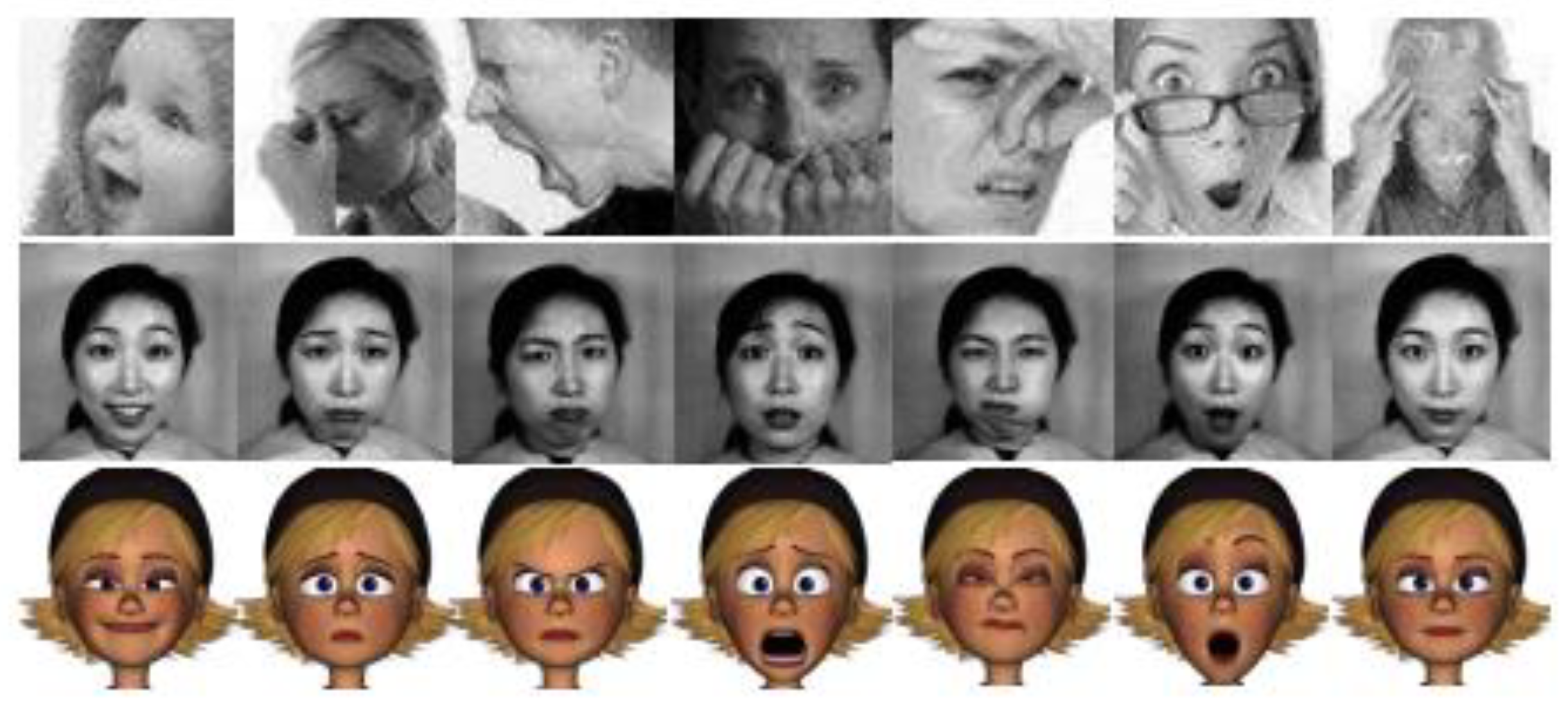
Figure 2.
Training Samples of the dataset.
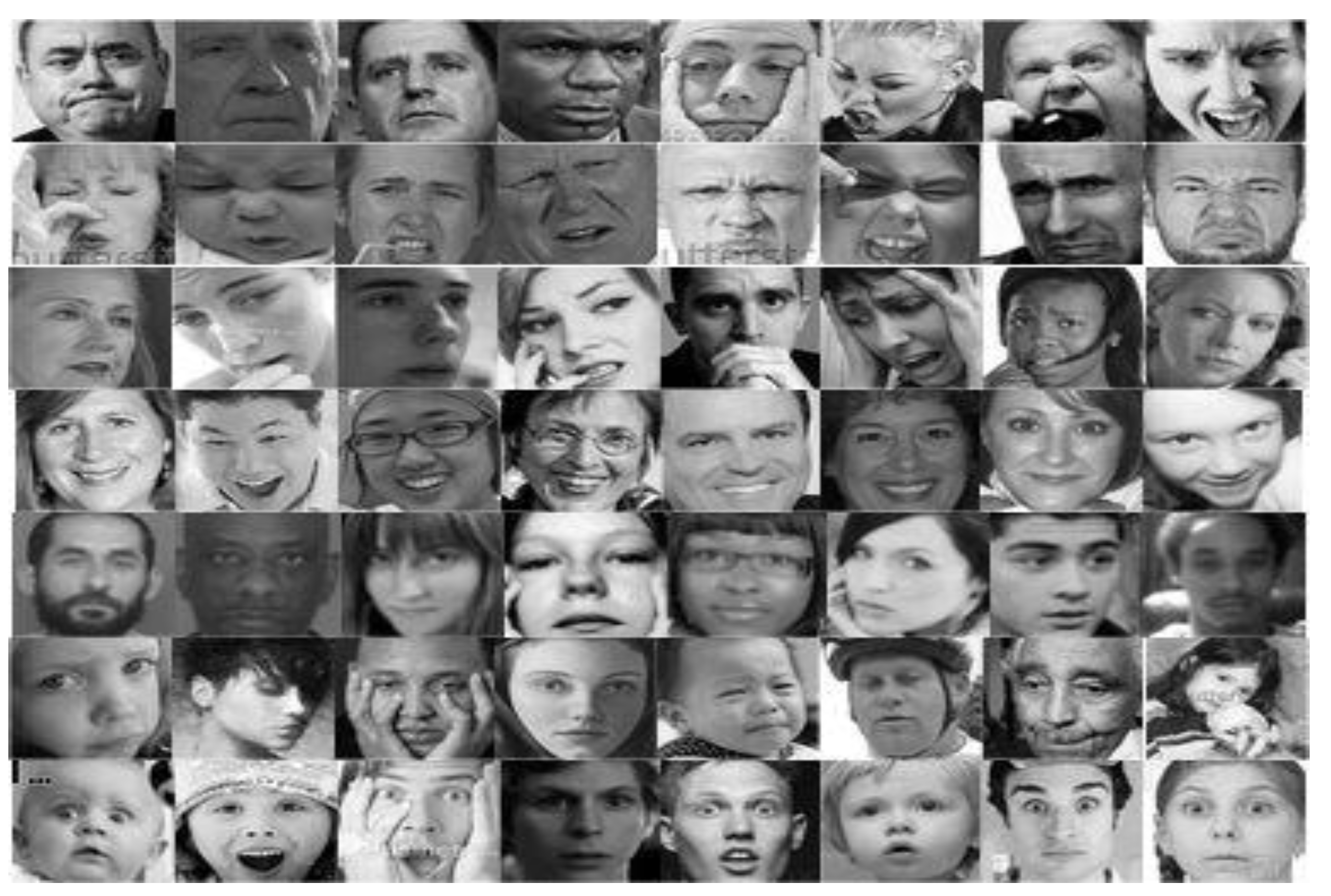
Figure 3.
Comparison of Machine Learning & Deep Learning model.
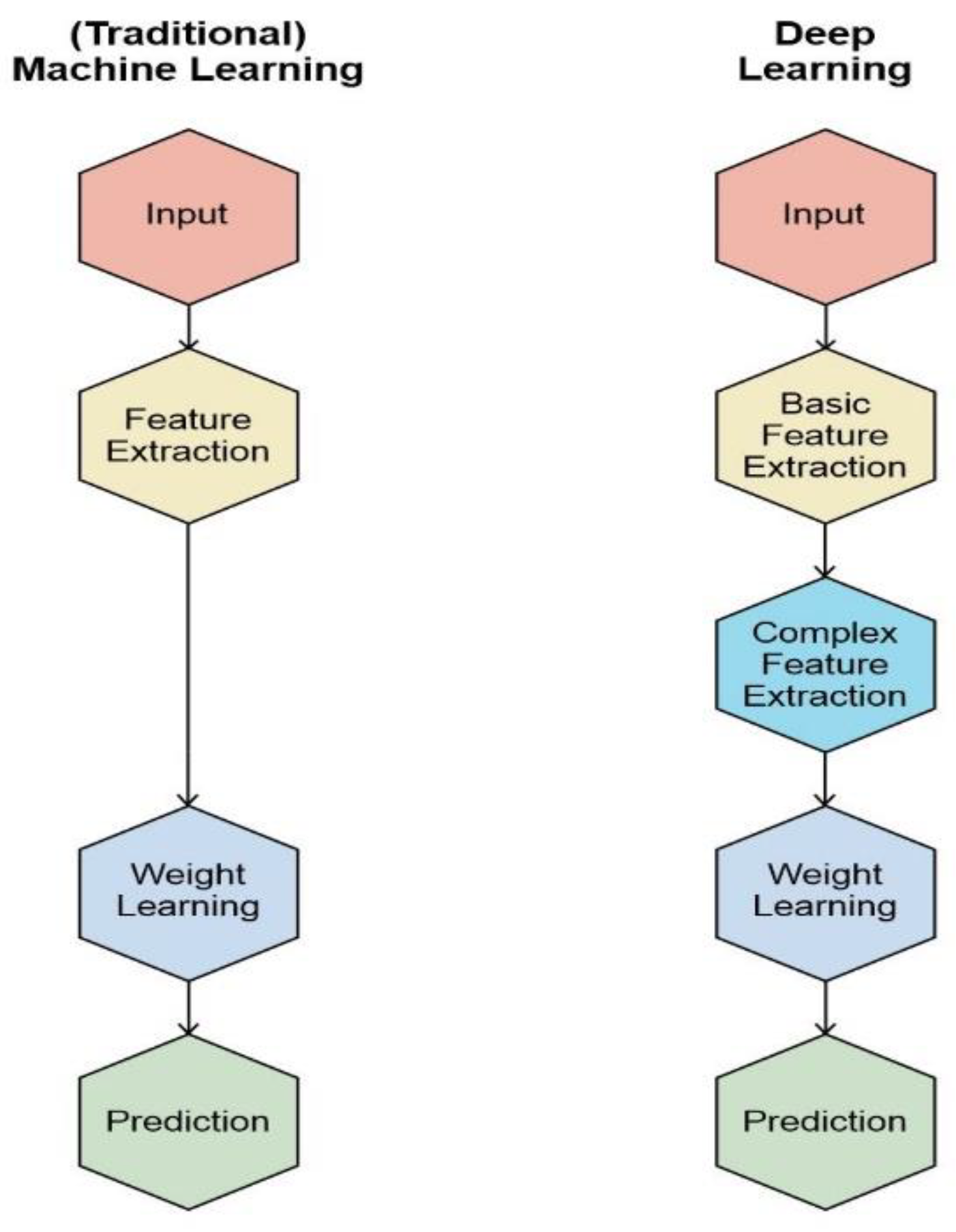
Figure 4.
Convolution Neural Networks and Fully Connected Neural Networks.
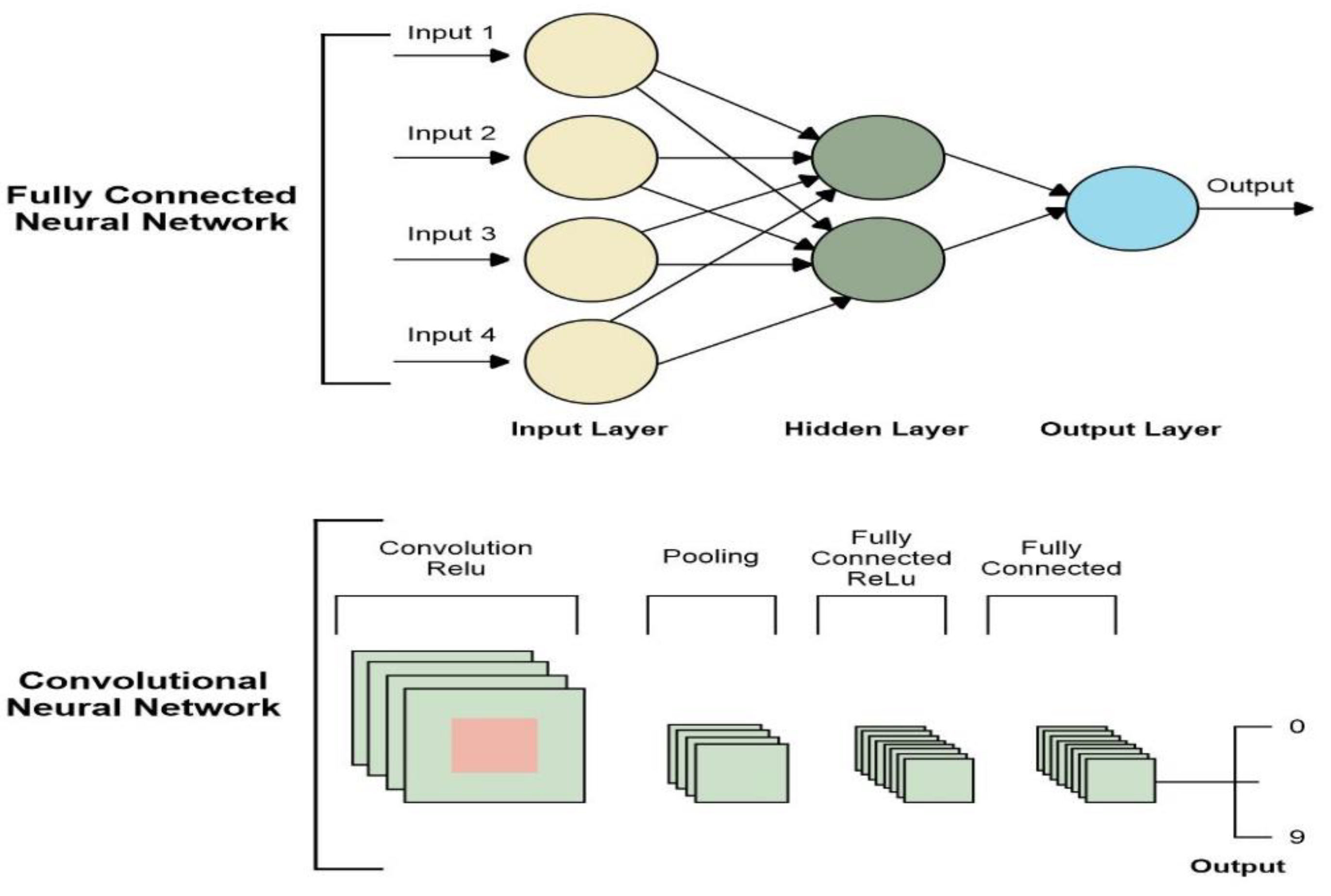
Figure 5.
The general architecture of the CNN-based model.
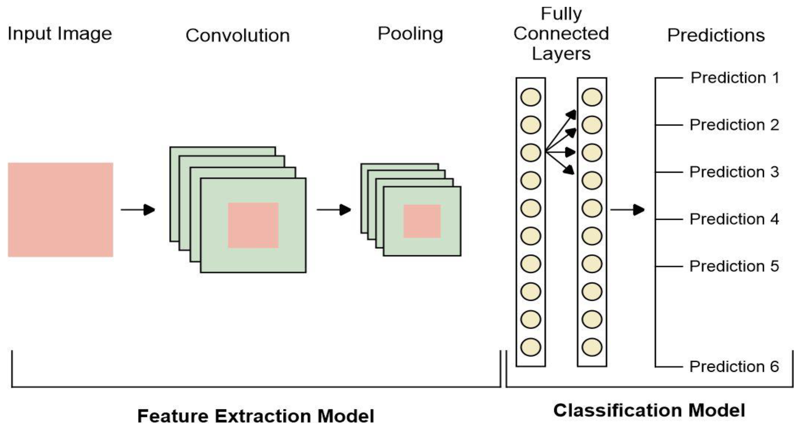
Figure 6.
Working architecture of Neural Search.
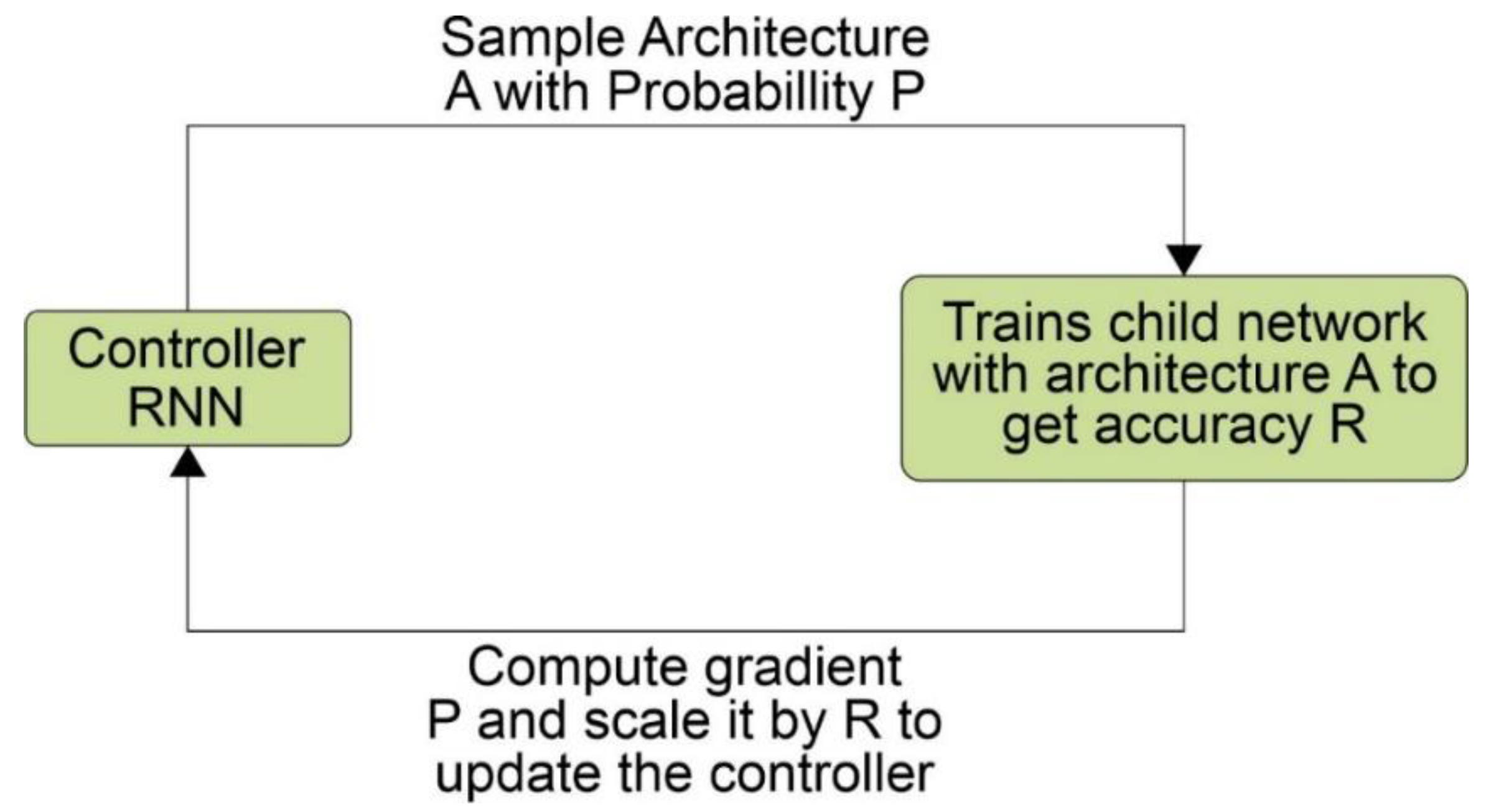
Figure 7.
Controller RNN in Network architecture.
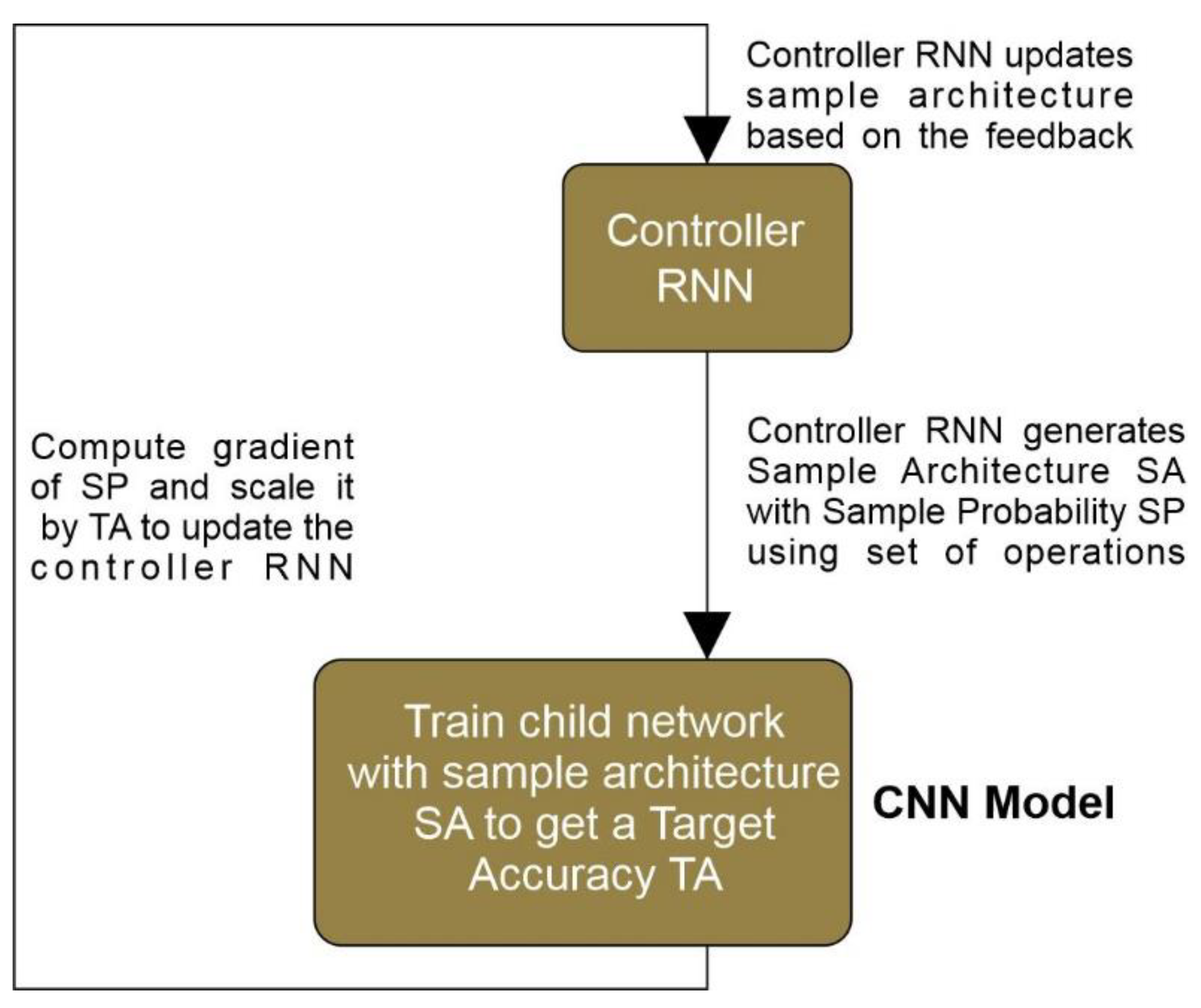
Figure 8.
Block formation of the proposed architecture.
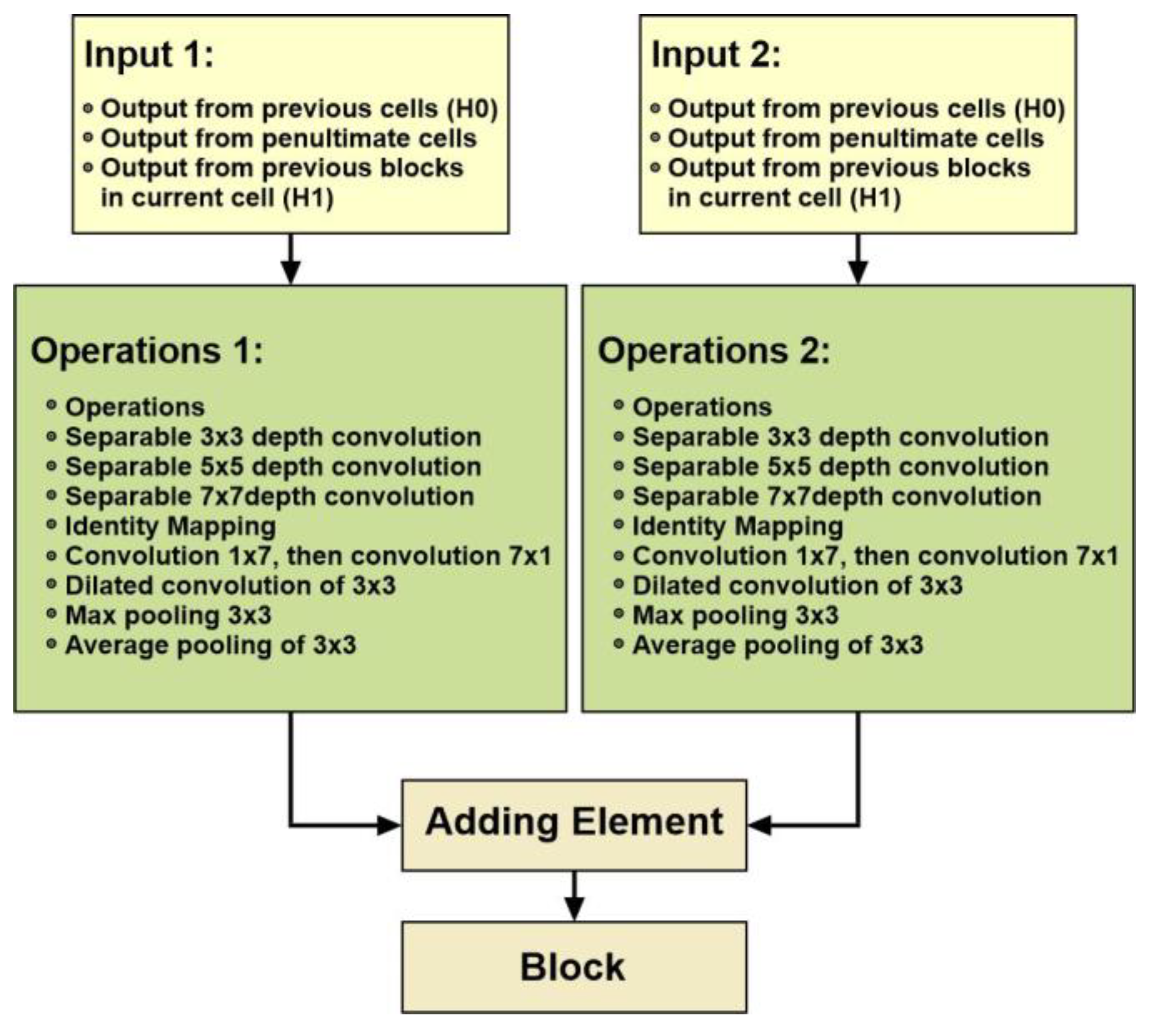
Figure 9.
Taxonomy of the proposed network’s architecture.
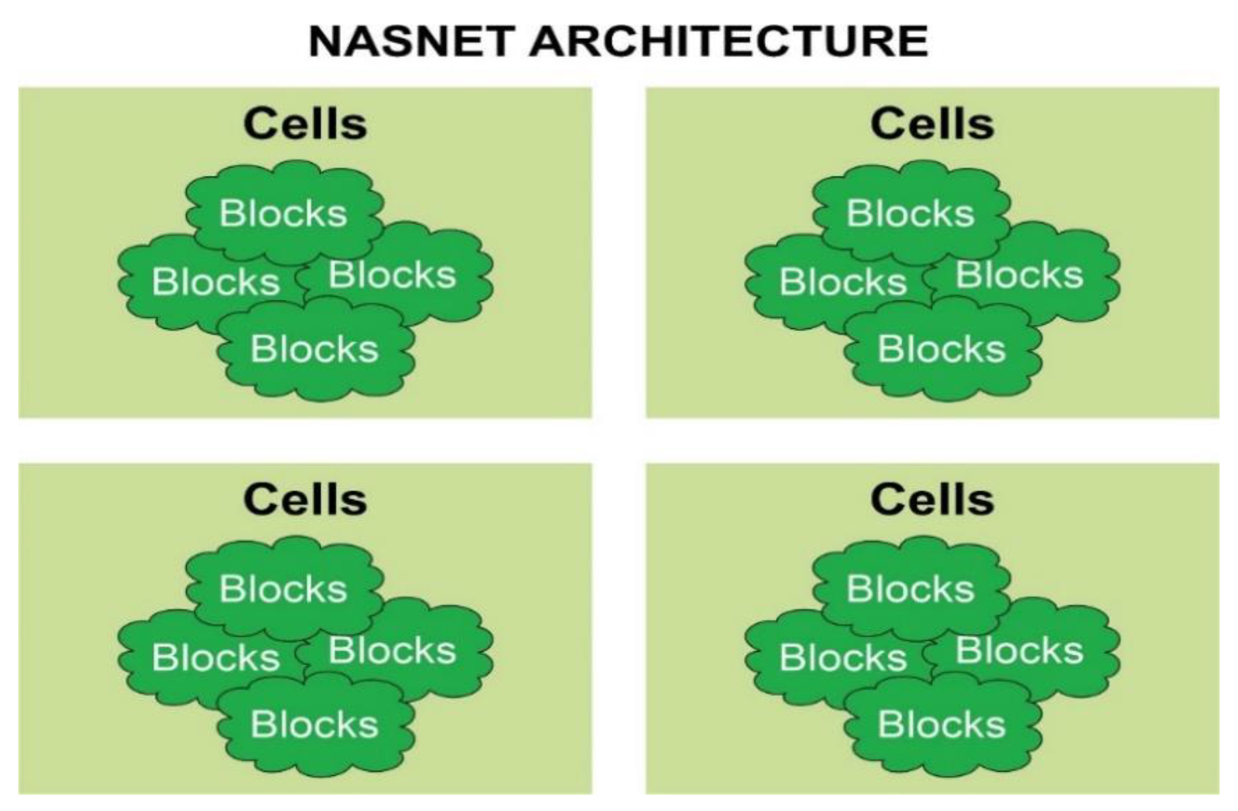
Figure 10.
Information about the Hidden States.
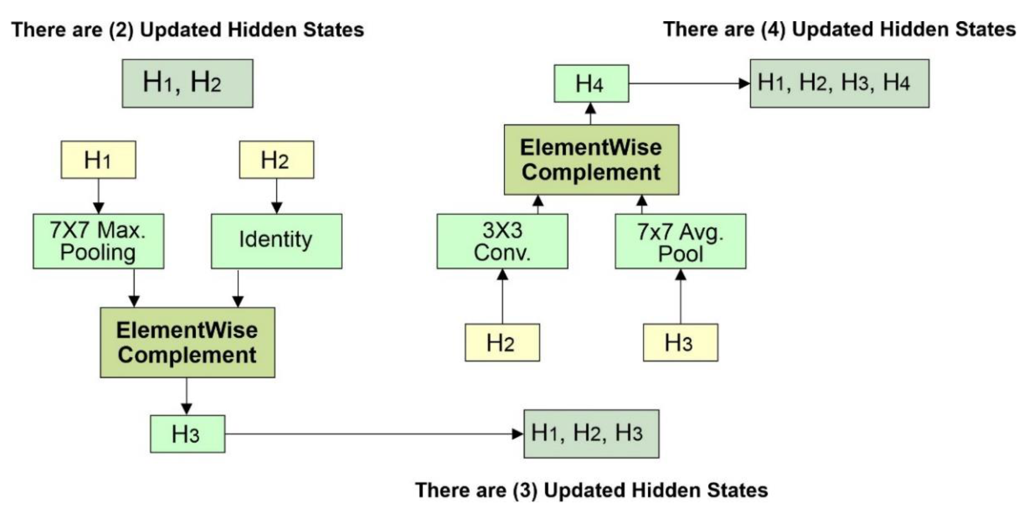
Figure 11.
Structure of Network search space.
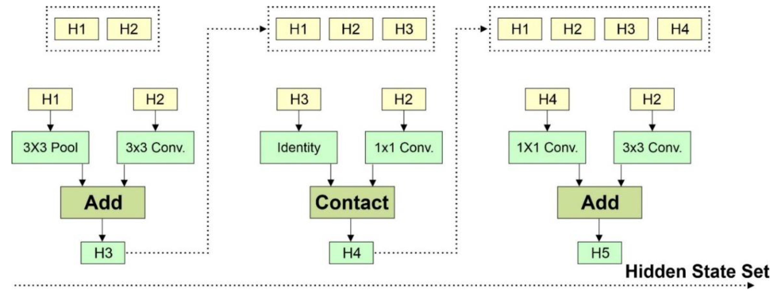
Figure 12.
The Proposed Architecture System.
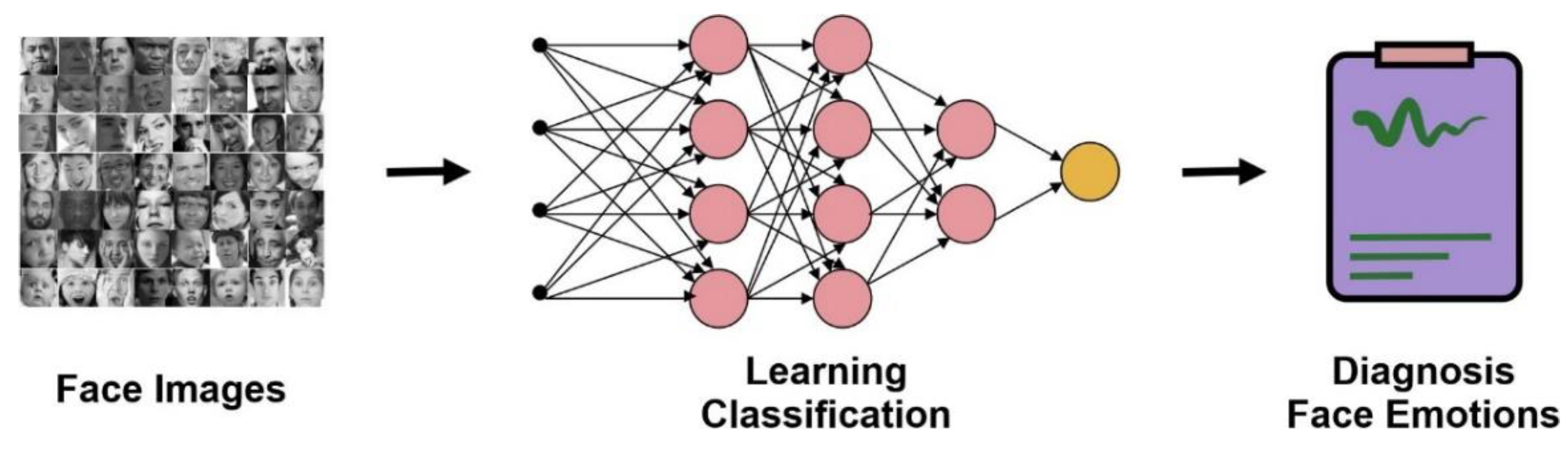
Figure 13.
Classified Samples of FER 2013 using the Proposed Model.
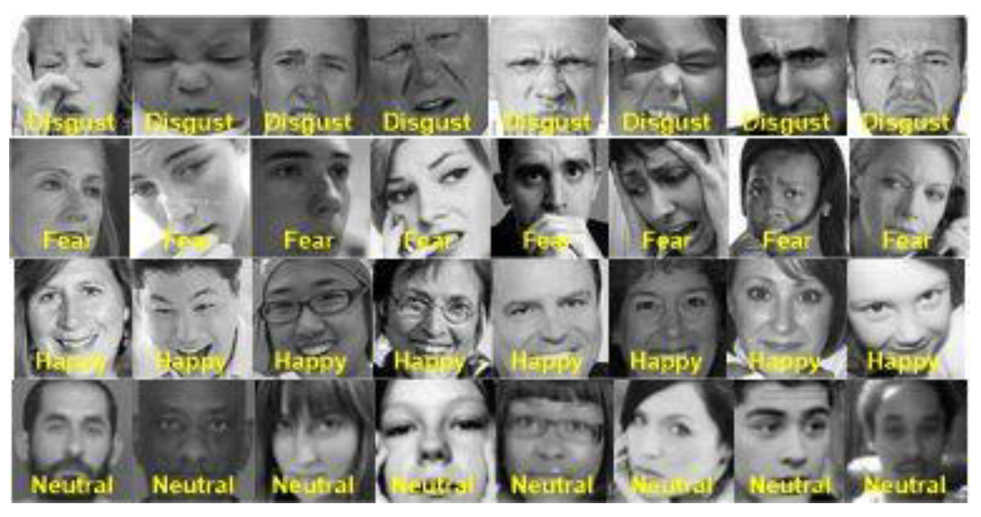
Figure 14.
Confusion Matrix over FER 2013 Test Data.
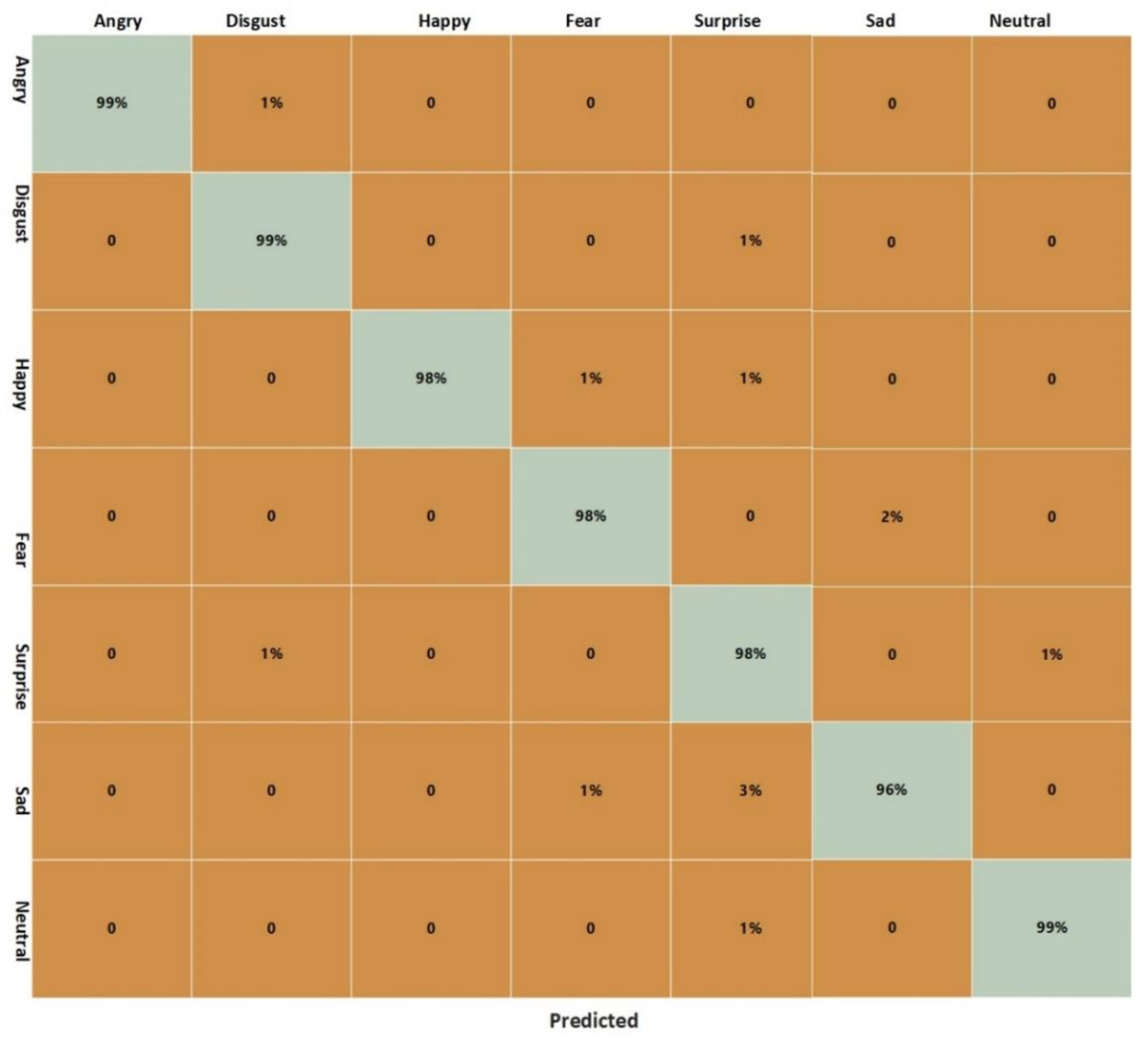
Figure 15.
CK+ Dataset Samples.
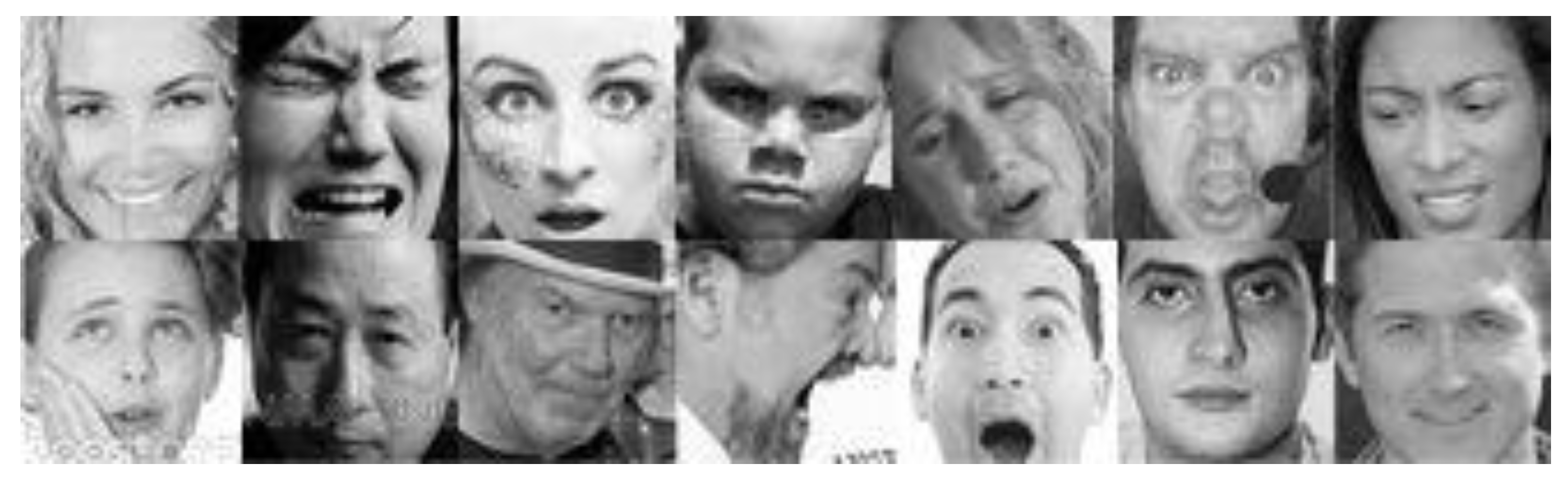
Figure 16.
ROC curve training data accuracy.
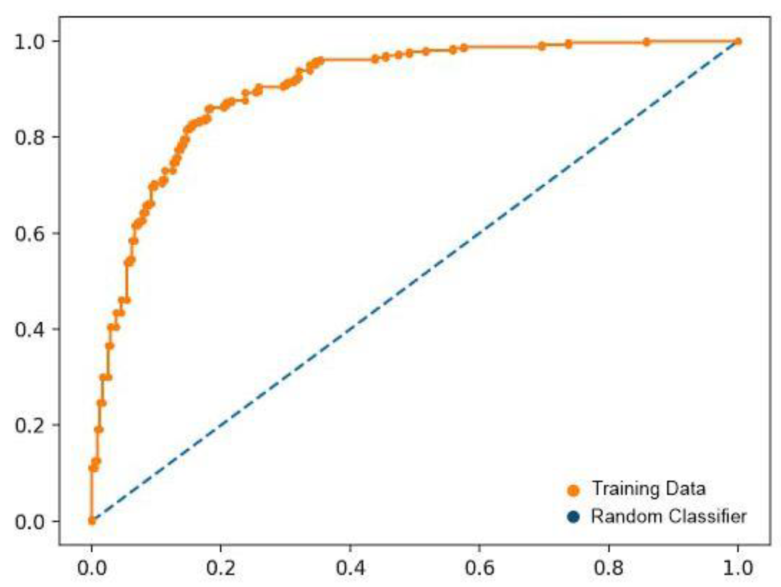
Figure 17.
Comparison with the existing models.
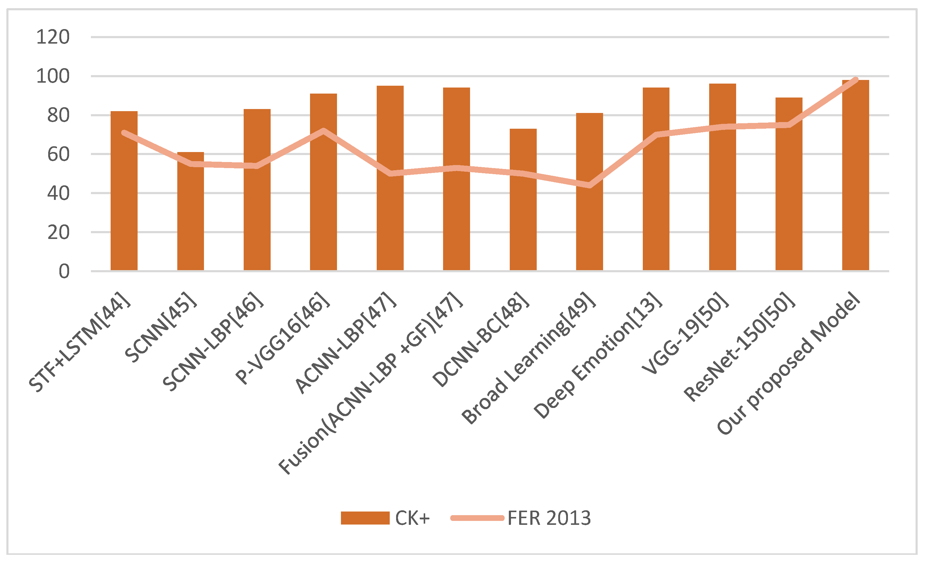

Table 1.
Detail of some existing FBR systems.
| Reference | Technique | Purpose | Results | Dataset | Accuracy |
|---|---|---|---|---|---|
| Wang et al. [26] | LeNet-5 | For the improvement of accuracy and to resolve the robust occlusion, ER | A reliable method has a high occlusion recognition score. | CK+ | 97.23% |
| Kaviya et al. [28] | Haar feature descriptor | Improvement of Recognition | The model shows that facial expression-related features have been learned better through CNN. | Custom Dataset and FER 2013 | 60% and 65% |
| Hussein et al. [29] | Adam optimizer and loss function | Improve the detection of emotions | The model identifies positive and negative emotions better than neutral ones. | CK+ and FER 2013 | 81% |
| Ravi et al. [30] | LBP and SVM | To differentiate CNN and LBP | The CNN model performs better than LBP for classification. | CK+, and YALE FACE | 97.32% and 31.82% |
| Ganapathy et al. [31] | LDA, SVM, MLP, DT, and ELM classify EDA signals. | Provides more stable features for dynamic EDA signals | The model proved that CNN classifies common expressions better under various health scenarios. | DEAP Database | 75% for arousal and 72% for valence |
| Ozean and Basturk [32] | PSO method for hyperparameter tuning | To prove the success of deep learning models | They increased the number of training samples and improved the performance. | ERUFER | 92.56% |
| Li et al. [33] | LBP with attention model | To decrease overfitting and generalization of the model during training | The model outperforms existing techniques but is suitable only for 2-dimensional samples. | FER2013 | 75.82%, |
| Meryl et al. [34] | Radial function(RBF) | For better accuracy | The accuracy of the CNN in RBF is evaluated. | FER 2013 | 95.4% |
| Mohan et al. [35] | DCNN | For the improved classification of feelings | Both holistic and local features will improve FER recognition. | FER 213CK+ | 78%97.9% |
| Agrawal et al. [36] | VGGNet and AlexNet | For the customized network to be trained and simplified, the implementation | The size of the kernel and total layers affect the accuracy. | FER 2013 | 65% |
| Ozdemir et al. [37] | LeNet CNN architecture | To attain an accurate model | A higher-quality model and real-time software for recognition. | JAFFE, KDEF, and custom | 96.43% overall |
| Otberdout et al. [38] | SVM with Gaussian Kernel with SPD manifest | To improve the efficiency of the FER system | Improved the FER system by employing the deep covariance descriptors. | Oulu-CASIAAFEW | 87%49.5% |
| Ameur et al. [16] | MBP | Improvement of the FR system’s performance | Gave an example of relative success over the LFW scheme as compared to other techniques. | Labeled Faces in the Wild (LFW) | 98.90% |
Table 2.
Dataset Details for Training and Testing.
| Class Label | Training Data Samples | Testing Data Samples |
|---|---|---|
| Happy | 6998 | 1801 |
| Angry | 3874 | 947 |
| Neutral | 5175 | 1199 |
| Disgust | 465 | 123 |
| Fear | 4107 | 1134 |
| Surprise | 3201 | 756 |
| Sad | 4790 | 1109 |
| Total | 28610 | 7069 |
Table 3.
Layers Architecture of the proposed Network.
| Convolution | III x I then III x I |
| Convolution | I x VIII then VII x I |
| Dilated Convolution | III x III |
| Average Pooling | III x III |
| Max Pooling | III x III |
| Max Pooling | V x V |
| Max Pooling | VII x VII |
| Convolution | I x I |
| Convolution | III x III |
| Depth Wise Separate Convolution | III x III |
| Depth Wise Separate Convolution | V x V |
| Depth Wise Separate Convolution | VII x V11 |
Table 4.
System's environment details.
| Hardware | Specifications |
|---|---|
| Computer | GPU Server |
| CPU | Intel Core i5, 4th generation |
| SSD Hard Drive | 256GD |
| RAM | 8GB |
Table 5.
Parameters details of the Proposed Network.
| Parameters | Value |
| No. of epochs | 25 |
| Batches Size | 16 |
| Learning Rate | 0.001 |
| Model Confidence Value | 0.25 |
Table 6.
Class-wise performance of the proposed model.
| Class | Precision (%) | Recall (%) | Accuracy (%) | F1-Score (%) |
|---|---|---|---|---|
| Angry | 96.8 | 97 | 99 | 96.90 |
| Disgust | 98.5 | 98 | 99 | 98.24 |
| Fear | 98 | 97 | 98 | 97.50 |
| Happy | 97.6 | 98 | 98 | 97.80 |
| Neutral | 100 | 99 | 99 | 99.50 |
| Sad | 97 | 96 | 96 | 96.50 |
| Surprise | 97 | 98 | 98 | 97.50 |
| 97.9 | 97.6 | 98.14 | 97.70 |
Table 7.
Comparison with Existing Models.
| Model | CK+ | FER 2013 |
|---|---|---|
| STF+LSTM[44] | 82 | 71 |
| SCNN[45] | 61 | 55 |
| SCNN-LBP[46] | 83 | 54 |
| P-VGG16[46] | 91 | 72 |
| ACNN-LBP[47] | 95 | 50 |
| Fusion(ACNN-LBP +GF)[47] | 94 | 53 |
| DCNN-BC[48] | 73 | 50 |
| Broad Learning[49] | 81 | 44 |
| Deep Emotion[13] | 94 | 70 |
| VGG-19[50] | 96 | 74 |
| ResNet-150[50] | 89 | 75 |
| Our proposed Model | 98 | 98.14 |
Disclaimer/Publisher’s Note: The statements, opinions and data contained in all publications are solely those of the individual author(s) and contributor(s) and not of MDPI and/or the editor(s). MDPI and/or the editor(s) disclaim responsibility for any injury to people or property resulting from any ideas, methods, instructions or products referred to in the content. |
© 2023 by the authors. Licensee MDPI, Basel, Switzerland. This article is an open access article distributed under the terms and conditions of the Creative Commons Attribution (CC BY) license (http://creativecommons.org/licenses/by/4.0/).
Copyright: This open access article is published under a Creative Commons CC BY 4.0 license, which permit the free download, distribution, and reuse, provided that the author and preprint are cited in any reuse.


