
Submitted:
13 September 2023
Posted:
14 September 2023
You are already at the latest version
Abstract
The paper proposes an approach to determine the optimal number of medical specialists in the region. According to the author's theoretical model, in order to maximize public welfare, the marginal contribution of the last physician recruited to the growth of the public utility function should be equal to the marginal cost of attracting him and providing conditions for his work. To empirically assess the contribution of physicians to the number of lives saved, the CVD mortality rate is modeled using the instrumental variable method. On average, a 1% increase in the number of cardiologists is associated with a 0.6% decrease in cardiovascular mortality. At the level of provision with cardiologists in the amount of 1 per 100 thousand people, their marginal contribution to the number of lives saved is not less than 129 per 100 thousand people, with a further decrease by 5 people with the increase in the level of provision by 1 unit. The use of the obtained results will increase the validity of managerial decisions and in determining the optimal level of doctors when choosing between alternative possibilities of spending money on hiring doctors of different profiles or other expenses, especially in the case of limited resources.
Keywords:
health care markets
; cardiovascular mortality
; health care workforce
; applied microeconometrics
; spatial econometrics
; instrumental variable method
; quasi-public goods
1. Introduction
Relevance. The present study attempts mathematical modeling and proposals of empirical applications based on the theory of public goods and methods of applied econometrics in industrial organization in the field of health care. In many countries of the world the state takes an active part in the formation and regulation of the market of health services [1]. At the same time, in such countries as, for example, Russia, the state system guarantees free access of citizens to the majority of the most common services in the sphere of health care on the basis of application of the mechanism of compulsory health insurance [2]. Profile authorities at the regional and federal levels are faced with the need to make decisions on the provision of medical services. We are talking about decisions related to the determination of the number of specialized doctors and medical staff, beds, as well as decisions in the field of personnel training, including the planning of the number of budgetary places in specialized educational institutions. But what is the basis for making decisions about the optimal number of doctors, for example, cardiologists, at the level of a particular region? To date, such decisions are made on the basis of federal regulations, which contain standardized average coefficients that determine the number of certain doctors per 100,000 people, taking into account the expected number of requests for medical services and the average appointment time [3]. These coefficients do not sufficiently take into account the characteristics of territories, for example, socio-economic status, demographic characteristics of the population. It is also about the fact that the characteristics of territories can lead to variations in the extent to which the number of doctors can influence mortality from a particular disease, and even to estimate the average impact, other things being equal, it is necessary to take into account the presence of observed and omitted variables, reverse causality and other econometric problems [4]. For example, according to Rosstat data, in the Penza region the mortality rate from cardiovascular diseases is 749 per 100,000 people, with a cardiologist supply rate of 12.4 per 100,000 people, while in the Nenets Autonomous District the corresponding mortality rate is less than 348 per 100,000 people, with a cardiologist supply rate of 6.8 per 100,000 people in 2019.
The level of development of the region itself, its geographical location, proximity to the federal center and specialized educational institutions are also important in the context of explaining the existing level of medical personnel supply [5]. In many respects, this will determine whether the region will be able to attract the necessary number of specialists for what is defined in the federal standards.
Thus, according to statistical data, there is a significant difference in the indicator of availability of cardiologists in the regions of the Russian Federation. For example, in such regions as the Jewish Autonomous Region, the Pskov Region, the Kurgan Region, and the Vologda Region, the number of cardiologists per 100,000 people is less than 6. And in such regions as the Astrakhan Oblast, North Ossetia, and St. Petersburg, the number of cardiologists per 100,000 people is more than 16 [6].
The currently used approach also does not allow us to answer the question of how many specialists should be employed to maximize the indicator of public welfare. There is also no way to compare managerial decisions related to the choice between doctors of different specialties, or between hiring an additional cardiologist or building a crosswalk near a school to reduce child mortality from accidents.
At the theoretical level, the research problem is defined by the existence of a gap that arises when trying to answer the question of what should be the optimal equilibrium volume of medical services in order to maximize the indicator of public welfare. In this paper we assume that the state, striving to maximize the indicator of public welfare, will strive to form the volume of supply of medical services as close as possible to the optimal one. And due to the peculiarities of the market of services in the sphere of health care, for example, the existence of long waiting lists due to underfunding, here and further we will assume that the supply of services in the sphere of health care in the optimal volume from the point of view of maximizing the indicator of public welfare will lead to the establishment of the equilibrium level of production and consumption of relevant services on the market as close as possible to the optimal volume. The existence of this gap is due to the fact that the state-guaranteed access to free health services in some cases leads to the fact that these services begin to be fully or partially characterized by the properties of public goods [7]. The state can strive for universal free access to health care because the consumption of health care services is a source of positive externalities, and thus without state guarantees or other forms of regulation, such as subsidizing health care services, underconsumption of health care services compared to the optimal level can be expected [8]. On the other hand, the fact that health care services begin to be characterized by the properties of public goods leads to the fact that other well-known problems arise, for example, the problem of the stowaway, which creates the preconditions for underfunding of the health care sector within the mechanism of compulsory health insurance [9]. For this and other reasons, the state has to make decisions both on the amount of additional financing of the health care sector and on the directions of spending the corresponding funds, which ultimately determines the volume of supply and, to a large extent, the equilibrium volume of specific medical services in the market under consideration.
In subsection 3.1 of this section we will consider a theoretical model for determining the optimal number of cardiologists based on the Samuelson equation [10]. However, in order to apply it in practice, it will be necessary to estimate the utility of hiring additional physicians in monetary terms, in order to compare it with the corresponding costs. In doing so, estimating the utility in monetary terms would require, on the one hand, an estimate of the cost of living, which in turn can take into account both an estimate under other things being equal and an estimate taking into account its expected duration and quality [11]. On the other hand, it is necessary to calculate the impact of the number of specialized physicians on the mortality rate from the respective disease area [12]. This is what will be the main focus of this paper.
Research question: how will the mortality rate of the population from cardiovascular diseases change, all other things being equal, if an additional number of cardiologists is hired in the regions of the Russian Federation? The most common research results in the literature demonstrate the negative impact of the indicator of availability of specialized medical personnel on the mortality rate from specific disease areas [13]. Such an impact can be explained by a significant reduction in the patient's waiting time in queues, which in turn can contribute to the receipt of timely medical care [14]. The importance of timely medical care is also important in the context of the presence of expected transaction costs in the perception of the potential patient, which has a significant impact on his or her decision to seek medical care. For example, the more a patient believes that there are long waiting lists and other transaction costs associated with staff shortages, the more he or she will be motivated to come to the hospital later, which, other things being equal, increases the likelihood of an adverse outcome [15]. Professional competition among specialists may also be important, so that in the case of an acute shortage of physicians with the relevant profile, they will have much less incentive to invest resources and make efforts to improve the quality of their work, for example by attending courses to improve their own qualifications, due to the fact that in the current conditions in the area, the employer will have an extremely strong incentive to retain the employee under any conditions.
In addition to the above-mentioned channels of influence of the level of medical personnel supply on the population mortality from the corresponding disease areas, it is important to emphasize the existence of conditions for the emergence of false positives and false negatives, which may lead to underestimation or overestimation of the corresponding influence and, to a certain extent, prevent the interpretation of the desired causal relationships.
False positives can occur for a variety of reasons, but they usually fall into one of the following categories: the presence of reverse causality, omitted variables, and peculiarities in the statistics used. In our case, the problem of reverse causality seems to be a significant one. The fact is that in some cases, in practice, there is even a positive correlation between the availability of medical personnel and mortality rates, which is largely due to the fact that in those areas where there is a high level of mortality from certain diseases, specialized authorities will try to increase the number of specialized medical personnel [16]. At the same time, even if a negative impact is detected during modeling, there is always a risk that this impact is underestimated due to the fact that reverse causality may exist. The underestimation of the corresponding negative impact can also lead to the problem of missing variables, for example, the variable characterizing the level of well-being and lifestyle of the inhabitants of a given area [17]. For example, it is known that a high income can lead to a person having a less physically active lifestyle, being more susceptible to the influence of bad habits, sleep disorders and being overweight [18]. On the other hand, high income and the associated level of development of the area will contribute to a higher indicator of availability of medical personnel that characterizes the area [19]. In combination, this will result in areas with both high mortality rates and high physician availability, creating a false-positive relationship. Existing inaccuracies in the statistical data may also lead to an underestimation of the negative impact of physicians on mortality. This may be due to the fact that in reality we do not observe the level of morbidity or mortality from a particular disease, but only indicators of detected morbidity or mortality. Thus, the availability of specialist physicians in an area has a greater direct effect on the recorded morbidity rate and a lesser effect on the recorded mortality rate. Therefore, it may be expected that areas characterized by a high availability of specialist physicians will be characterized by a higher level of recorded mortality from the corresponding diseases [20]. On the other hand, high availability of specialists may in some cases be associated with false diagnoses, which may also contribute to an increase in detected morbidity and mortality in the area.
False negatives may also be associated with omitted variables. For example, in practice, it is quite difficult to assess factors related to cultural aspects that characterize the attitude of the inhabitants of a given territory towards their health at the regional level. At the same time, an attentive attitude of the inhabitants of the region to their own health can lead to the fact that they are more likely to lead a healthy lifestyle, for example, to eat properly, to lead a physically active lifestyle, which will contribute to the reduction of the indicator characterizing the mortality rate from a particular direction of the disease [21]. At the same time, people who pay attention to their own health can also pay attention to issues related to the prevention of certain diseases, for example, in terms of early visits to doctors, which will also contribute to the increase in demand for medical services in the territory and create favorable conditions that contribute to the increase in the number of medical personnel [22]. As a result, there will be areas with both low mortality and high availability of specialists, but it will not be the doctors themselves, but first of all the attitude of the population to its own health. Similar reasoning can be given when analyzing the influence of the parameter of the level of medical literacy of the population, which can not always be expressed as an indicator of the level of education in general [23]. The indicator of the level of development of the territory can also act as a missing variable. On the one hand, a more developed territory is more likely to have high rates of availability of specialized doctors, while it is important to note that it is also more likely to have lower mortality rates, for example, due to preventive measures such as popularization of sports, access to quality food, medicines, opportunities to spend leisure time and organize quality recreation [22]. These circumstances may also contribute to inaccurate estimates in the absence of relevant data.
The above-mentioned reasons for the existence of false-negative and false-positive relationships are prerequisites that can potentially lead to underestimation or overestimation of the influence of indicators characterizing the impact of the level of availability of medical personnel on indicators characterizing the mortality rate of the population from the relevant disease areas.
Scientific novelty of the study. First, an approach to determining the equilibrium volume of services in the sphere of health care on the example of the supply of cardiologists, which differs from the existing ones by comparing the benefits and costs of hiring additional doctors, allowing to ensure the maximization of the indicator of public welfare, as well as the possibility of comparing the returns of decisions related to the recruitment of doctors of different profiles, as well as costs of non-medical nature, leading to the saving of human lives. Secondly, an econometric model for assessing the impact of the indicator of medical personnel availability on the indicator of mortality from specific disease areas, using the example of cardiovascular diseases, which differs from the existing ones by using a quasi-experimental method of estimation based on the author's instrumental variables, allowing to overcome the influence of econometric problems, in particular the problem of reverse causality and missing variables. Third, an approach to the design of instrumental variables for the application of quasi-experimental econometric methods for solving the problems of causal impact estimation is formed, which differs from the existing ones by using various modifications of spatial matrices and spatial econometric methods, including those that allow us to form arguments in favor of their exogeneity.
Thus, this study is aimed at developing approaches to improve the accuracy of estimates that characterize the impact of the indicator of availability of specialized medical personnel on the mortality rate of the population from specific diseases, which in turn allows us to implement an approach to determine the volume of supply of services in the field of health care based on the comparison of benefits and costs of its provision. The accuracy of the relevant estimates may allow the use of management decision support systems, which, among other things, will significantly improve the efficiency and targeting of relevant decisions, due to the possibility of forecasting and comparing the impact, including at the interagency level.
Structure of the paper. In the section "Introduction" the field of the research problem is presented, the research question is formulated and the relevance of the work is outlined. The "Literature Review" section summarizes the key findings in the context of the research question. In the section "Methods" the description of the theoretical model is given, on the basis of which the approach to answer the question about the optimal volume of supply of services in health care using the number of specialized cardiologists as an example is proposed, the tools for its empirical realization are suggested, including the tools of applied microeconometrics, models of spatial econometrics, the data are described, and the justification of the quasi-experimental method used in the work is formed. The section "Results" describes the main indicators in regression equations obtained in the course of econometric modeling. The section "Discussion" forms the main limitations of the study, compares the obtained results with those already known in the literature, and provides a discussion of the directions of their application in practice. In the section "Conclusion" the main results are formed, the theoretical and practical significance of the study is assessed, and directions for further research are formed.
This study contributes to the theoretical literature that discusses approaches to determining the optimal level of service provision in quasi-public goods markets using the example of the market for health care services [24,25]. It also contributes to the literature in the direction of refining empirical methods for assessing the contribution of health care financing policies to reducing population mortality, using cardiovascular disease as an example [26].
2. Literature Review
2.1. Health Services as a Quasi-Public Good
The debate about whether health care is a public or private good is still open. Fisk addresses this controversy in an article [27]. If health care is viewed as a commodity distributed by the market, then it is a private good. If health care is considered a public good, then its distribution requires a broadly consensual policy. The author believes that a healthy society can only be achieved through health care based on the principle of solidarity. This view is shared by Carsten [24], who argues that health care cannot be sold in the same way as health insurance. At the same time, the author notes the existence of market failures due to the inability of some people to get health care at the right time or when they need it most. In such cases, the market fails to provide the optimal amount of supply, leading to externalities. The author points out that such a problem can be solved by providing universal financial access to health care through insurance or mandatory employer contributions, as well as public benefits and subsidies. Anamoli, on the other hand, argues that public health care should be concerned only with the provision of public health services, which clearly separates it from private health care [28]. However, in another paper [25], the author extends Anamoli's concept and argues that attention should also be paid to water purification and air pollution control. Dees shares this view and believes that only the state can provide clean water and air, as well as universal access and free medical services [29]. It can be seen that the authors do not come to a clear answer about what public health should be. Moreover, pure public health does not currently exist. There are boundaries between public and private goods that differ depending on the chosen model of health care. In this case, public health can be considered a quasi-public good.
2.2. Factors Influencing Mortality from Cardiovascular Disease
The influence of various factors on mortality and morbidity from cardiovascular disease is the subject of constant attention by the medical and scientific community. Hypertension is one of the major causes of cardiovascular disease and is increasing worldwide. One study [30] investigated the causal relationship between blood pressure and cardiovascular disease. The authors used Mendelian randomization, which uses measured gene variability to examine causality as an instrumental variable. Positive associations were found for all cardiovascular diseases, supporting the findings that the lower the blood pressure, the lower the risk of cardiovascular disease. In another study [31], the authors used the Cox model to assess the risks of increased systolic and diastolic blood pressure, heart rate on the manifestations of cardiovascular disease. It was found that elevated systolic blood pressure had a large effect on angina pectoris, myocardial infarction, and peripheral arterial disease, and elevated diastolic blood pressure had a large effect on abdominal aortic aneurysm. Elevated heart rate was more associated with peripheral arterial disease.
Multiple studies show that obesity is associated with cardiovascular disease. Nordestgaard et al. [32] tested the association between body mass index and the risk of coronary heart disease. The authors hypothesized that control variables such as smoking, alcohol consumption, education, annual income, blood pressure, gender, and age might disrupt the association between dependent and key factors. To address this problem, they used the instrumental variables method. The results showed that every 4 kg/m2 increase in BMI increased the risk of coronary heart disease by 26%, and the instrumental variables method revealed a 52% increase in risk. A study by Larsson et al. used the Mendelian randomization method to assess the association between body mass index and 14 cardiovascular diseases. Data from the UK Biobank from 2006 to 2010 were used for the study. The sample included about 500,000 adults aged 40-69 years. The results of the study showed that high BMI is associated with an increased risk of aortic valve stenosis and most other cardiovascular diseases [33].
Studies suggest that type 2 diabetes may have a significant impact on cardiovascular disease morbidity and mortality. In one article [34], the relative risk of cardiovascular disease was twice as high in men and three times as high in women with diabetes compared to those without diabetes. In a study [35], estimates from proportional hazards regression analysis showed that the risk of death from cardiovascular disease was higher in men with diabetes than in men without diabetes, adjusting for various control factors.
Smoking is also an important risk factor. For example, smoking a single cigarette dramatically and temporarily increases blood pressure by activating the sympathetic nervous system. Exposure to tobacco smoke increases the risk of coronary plaque rupture and causes coronary artery spasm. A non-linear relationship between daily cigarette smoking and coronary heart disease has also been observed. In addition, there is no evidence that other tobacco products are safer than conventional cigarettes [36].
A meta-analysis [37] summarized the results of the association between alcohol consumption and the risk of heart failure. A moderate inverse association was observed between low alcohol intake and the risk of heart failure. In addition, the results of the meta-analysis showed that previous alcohol consumption was associated with an increased risk of heart failure. The article [38] performed a systematic review of the literature on the use of Mendelian randomization to identify causal relationships. Due to the heterogeneous application of the method in the reviewed studies, it is not yet possible to draw conclusions about the causal role of moderate alcohol consumption. However, excessive alcohol consumption is a known factor in mortality and the burden of cardiovascular disease [39].
A number of studies indicate an association between low education, low income and increased risk of heart and vascular disease. A study [40] examined the effect of income and education on mortality from acute myocardial infarction. The study used the Cox proportional hazards model, adjusting the data for sex, age, marital status, and other factors. Mortality in the first 30 days after hospitalization was 7% among patients aged 30-64 years and 15.9% among patients aged 65-74 years. After 30 days of hospitalization, mortality was 9.9% and 28.3%, respectively. The adjusted relative risks of mortality in the first 30 and subsequent days of hospitalization in young low-income versus high-income patients were 1.54 and 1.65, respectively. The situation was similar for education, 1.24 and 1.33. In elderly patients, the adjusted relative risks of mortality in low-income versus high-income patients were 1.27 and 1.38, respectively. Meanwhile, elderly patients with high and low levels of education did not differ in mortality. Ho et al. evaluated the association between education level and the risk of acute myocardial infarction [41]. The authors used a Cox model to assess the association between education and outcomes in the study. They also adjusted for demographic factors to test for changes in the association between education and outcomes. In the unadjusted analysis, they found that low education was associated with a higher risk of cardiovascular problems over the course of a year. However, after adjusting for risk, the association between education and death was statistically insignificant. Nevertheless, the risk of developing cardiovascular problems remained significantly higher in the group of people with low levels of education. Hamad et al. conducted an experiment to test how education affects various aspects of cardiovascular disease and associated risk factors. They used the instrumental variables method to determine the effect of education because there was doubt whether education was the real cause of cardiovascular disease or correlated due to reverse causality. The instrument chosen to measure education was the School Education Act. The authors also used fixed effects models. Results from the instrumental variables method showed that increased education was associated with reductions in smoking, depression, triglyceride levels, heart disease, and improved HDL cholesterol levels. However, increased education was also associated with increases in body mass index and total cholesterol levels. When fixed effects were accounted for in the model, these factors became statistically insignificant [42].
The authors in [43] examined the effect of marital status on outcomes in patients with coronary heart disease and at high risk of developing this disease. They used Cox proportional hazards regression to determine the relationship between marital status and outcomes, adjusting for sex, race, diagnosis of arterial hypertension, diabetes mellitus, body mass index, smoking history, education, employment status, and other factors. There were 1,085 deaths from all causes, including 688 from cardiovascular disease and 272 from myocardial infarction. Unmarried people had a higher risk of all-cause death (1.24), cardiovascular disease (1.45), and myocardial infarction (1.52) compared with married people. A similar situation was seen in divorced (1.41) and widowed (1.71) patients. The authors note that the results remained significant after adjusting for medications and other socioeconomic factors.
Gallo et al. used 10-year follow-up data to estimate the effect of job loss among people over age 50 on subsequent risk of myocardial infarction and stroke. The key variable was a binary measure of involuntary job loss due to business closure, plant closure, or layoff. Socio-demographic status, economic variables, and comorbidities were used as control variables. Using Cox proportional hazards regression, the authors found that the risk of myocardial infarction and stroke was twice as high among those who lost their jobs involuntarily compared with those who were employed. For many people, job loss is an extremely stressful situation that can trigger cardiovascular disease [44].
The results of the study showed that there is a causal relationship between anxiety, depression and acute myocardial infarction and sudden cardiac death [45]. On the other hand, positive psychological aspects such as optimism have been identified as contributing factors to cardiovascular health [46].
Studies [47,48] have found a positive association between air pollution and cardiovascular mortality. Extreme heat and cold have also been found to influence the risk of cardiovascular disease [49,50]. Sex, age, and race differences, low physical activity, and urbanization are also considered significant factors influencing cardiovascular disease mortality and morbidity in the literature [51,52,53,54,55].
2.3. Econometric Issues in Assessing the Influence of Physicians on Cardiovascular Disease Mortality Rates
A number of studies have been conducted in the scientific literature on the impact of the number of physicians on cardiovascular disease mortality. Simionescu et al. related the number of deaths from cardiovascular disease to per capita health care expenditures, the number of public hospitals with cardiology departments, and the number of cardiologists. The authors used Bayesian linear regression models for time series at the national level and panel data models with fixed effects at the regional level to control for unobserved variables. The Bayesian model showed a negative effect on the number of deaths, and an increase in the number of physicians and hospitals was associated with an increase in mortality. The fixed effects model showed that, on average, an increase of one cardiologist reduced mortality by one. However, an increase in the number of public hospitals was positively associated with mortality. The authors conclude that the results differ at the national and regional level because of the influence of the number of cardiologists [56].
Another study examined the relationship between access to health care and preventable mortality from several diseases, including cardiovascular disease. The authors used three models: a pooling model, a fixed effects model, and a random effects model. The random effects model was the appropriate model for estimating variables on mortality in men. The researchers note that increasing the number of pediatricians in the region by one would increase the regional mortality rate by 3,885 deaths per 100,000 population. The situation is similar for general practitioners (1,482). The other two statistically significant variables (number of pharmacies and number of specialists) have negative relationships with coefficient values of 3.904 and 0.3777. For women, the random effects model was appropriate. An increase in the number of general practitioners and dentists would increase the mortality rate by 0.724 and 0.557 per 100 thousand population, respectively. The number of gynecologists, pharmacists and specialists have negative estimated coefficients [57].
The contradictory results are due to two econometric problems: the omitted variable problem and the reverse causality problem. While the authors partially solved the omitted variable problem by using fixed and random effects models, the reverse causality problem is still important for analyzing the relationship between the number of physicians and mortality. It is possible that regions with higher mortality have more physicians not because their presence leads to lower mortality, but because there is a greater need for medical personnel due to high morbidity and mortality. This problem can be partially addressed using instrumental variables techniques.
One study [58] evaluated the impact of different medical services on hospital admissions. One of the factors was physician density. The authors solved the problem of omitted (unobserved) variables by using spatial autoregressive analysis. In addition, the authors used the instrumental variables method to solve the problems of omitted variables and reverse causality. The authors used the medical student factor as an instrument, reasoning that most graduates stay and work in the region where they studied after graduation.
Sundmacher et al. examined the effect of regional differences in the provision of health services on the types of preventable cancer deaths. The dependent variable was the age-standardized non-negative mortality rate. The reason for using the instrumental variable method was that the distribution of physicians was not strictly regulated until 1993. There may have been incentives for physicians to move to areas with high and low incidence rates of these cancers, resulting in reverse causality. In addition, there are omitted variables that correlate with both the incidence of mortality from preventable cancers and the supply of physicians. In Germany, individuals who refuse military service can choose to serve in the national system. Most of these positions are in the health sector, so the total number of such positions per 100,000 population was used as an instrument. The results showed that an additional 10 physicians would reduce the incidence of acute cancer by about one case every five years [59].
A study [60] examined the existence of physician-induced demand for hypertension services in Ghana. A positive correlation between these indicators would indicate an artificial demand for these services, so the authors assume the existence of endogeneity. The authors use district population size and male population ratio as instruments, which only affect demand for health services through the ratio of doctors to population. A high male population ratio indicates the presence of mining and cocoa farming. This in turn indicates a vibrant local economy and high purchasing power. The population of the district indicates a high availability of amenities such as good schools for the children of doctors, stable supply of electricity and water, and the presence of high economic activities. In addition to the instrumental variables method, the authors use a fixed effects model. The results suggest that a 1% increase in physician density increases visitation by 0.75%. This supports the authors' hypothesis that there is an artificial demand for health services in Ghana.
Subramanian et al. examined the effect of physician density on infant mortality. The authors noted the presence of endogeneity problems due to omitted variables and reverse causality. To address these issues, the authors used the instrumental variables method. The authors used lagged physician density as the instrument. The results of the study showed that an increase of one physician per 1000 population reduces infant mortality by 15% over five years and by 45% in the long run [61].
3. Methods and Data
3.1. Theoretical Model for Determining the Optimal Number of Physicians
Need for government intervention. The consumption of health services by the population leads to positive externalities. For example, healthier individuals are more likely to be more productive, start new businesses, make scientific discoveries, and achieve other successes that benefit the rest of society [62]. The presence of positive externalities in consumption means that market equilibrium without government intervention will result in the amount of services consumed being less than the optimal amount in terms of maximizing public welfare. This happens because individual economic agents, when deciding to purchase and consume an additional unit of a good, consider only the personal utility received, which is less than the utility for the whole society, leading to underconsumption. There are various ways in which the government can intervene to correct such "market failures", such as subsidies [63]. In practice, instead of subsidizing each individual patient, the state subsidizes medical organizations, which, together with the presence of compulsory health insurance, forms the contours of modern health care systems in countries with models similar to the health care system in the Russian Federation [64].
Consequences of state intervention. In fact, the actions of the state lead to the fact that health services begin to be characterized by the properties of public goods. We are talking about characteristics such as non-excludability and non-competitiveness [10]. The fulfillment of these characteristics can be interpreted in different ways. For example, non-excludability implies that it is impossible to provide a service to one consumer without providing it to all others, and to some extent universal free medical care implies this. On the other hand, the non-competitiveness property is satisfied in a more truncated form, because when a doctor sees a patient, he cannot see a second patient at the same time. In this case, the second patient is still seen, but at a later time, which in practice is characterized by long queues at the doctor's office [65]. For such services, the concept of quasi-public services is often used in the literature [25]. In fact, it would be more accurate to consider the system as a whole as a quasi-public good, rather than each individual service in the health care system. And as the main characteristic we can consider its throughput capacity per unit of time. For example, if there are 20 doctors working in the system, they can serve a larger number of patients with less waiting time than if there are only 10 doctors working in the system, all other things being equal. This is analogous to a public swimming pool with free access but queues. In the case of health care, the size of the system, i.e. its capacity, is determined to a greater extent by the state. In fact, we are talking about the equilibrium volume of services provided, and although it is determined by the interaction of supply and demand, the peculiarities of the market, combined with the fact that there is a deficit of services on the market, which can be confirmed by the presence of queues, leads to the fact that the state, by influencing the supply of services, for example by increasing the number of doctors, directly affects the equilibrium level of consumption. The state determines the interest rate that characterizes the level of payments to the mandatory health insurance funds and participates in the additional financing of the health care system [66]. The role of additional financing is growing, in part because of the problem of "stowaways" resulting from free access to the health care system regardless of the patient's own contribution.
Approach to determining the optimal number of doctors. In the literature, it is common to use Samuelson's equation [10] to determine the optimal quantity of public goods in the context of maximizing public welfare. According to it, the volume of public goods is considered optimal if the total marginal utility of all consumers is equal to the marginal cost of its production. It is assumed that the conditions are met, according to which an increase in the volume of public goods always leads to an increase in the utility of its consumption, but each additional unit leads to an increasingly smaller increase. In this case, the costs increase at an accelerated rate as the volume of public goods produced increases.
Let the production of health care services be determined by the required number of specialized doctors. All other costs related to medical personnel, equipment, and other infrastructure are determined by the number of doctors. That is, from the point of view of society, we have a cost function of the form (1) and a utility function of the form (2). Then, the public welfare indicator can be expressed by formula (3), and the condition for maximizing the level of public welfare is given by formula (4).
where, y is the number of physicians, through which the volume of services provided, the scale or throughput of the health care system is determined.
Formula (4) is a necessary and sufficient condition for maximization, in view of the corresponding properties of the cost and utility functions, namely v'(y)>0,v''(y)<0 and c'(y)>0 c''(y)≥0 for any y>0, c(0)=0. The economic interpretation of the introduced properties of the considered functions is as follows. Each additional physician will bring additional benefits, but the magnitude of these benefits will decrease. Even if the amount of equipment and other infrastructure also increases, the intuition may be that doctors will initially help patients with simpler diagnoses and treat more and more severe cases, so that each new doctor will face more difficulties, so that the contribution of each additional doctor to saving lives will decrease over time, although it will remain positive. In terms of costs, hiring an additional physician and providing him or her with a work environment will always incur additional costs, as more resources will be expended to find new qualified personnel. This may be due, for example, to the limited number of personnel in the area, which will require more effort and resources to attract new personnel, particularly to cover transportation and other transaction costs.
For simplicity, the utility function is given for society as a whole, without distinguishing between the utilities of individual patients and externalities. This is due to the fact that in practice it is rather labor-intensive to derive the utility functions of individual patients or the influence of external effects, and therefore the paper proposes an alternative way of estimating utility.
Let us give an economic interpretation of formula (4). If is fulfilled, it will mean that the last hired doctor still brings more benefits to society compared to the costs, and therefore, taking into account the considered properties, it is necessary to hire one more doctor, i.e. there is an underproduction of services in health care. That is, the indicator of public welfare can be increased by increasing the number of doctors. If is fulfilled, it will mean that hiring the last doctor has brought more costs to society than benefits and, therefore, there is an overproduction of services. And only at that number of doctors, when the equality of marginal utility and marginal cost functions is ensured, the maximization of the indicator of public welfare will be achieved.
In order to use formula (4), it is necessary to calculate the value of marginal cost, which is beyond the scope of this study, but does not seem difficult in any case, given the available information on current and potential costs. It is also necessary to obtain the function of marginal social utility, and here it is proposed to express it in the form of the product of the index characterizing the increase in the number of lives saved in case of hiring an additional doctor by the cost of one life saved. () (5). Then equation (4) takes on the form of (6). The question of estimating the cost of a life saved is also beyond the scope of this paper and can be considered both in a simple form, other things being equal, and taking into account its expected duration, qualitative characteristics, which is relevant, for example, when choosing between doctors of different profiles, medical procedures, and other alternatives.
The main empirical focus of this paper is to derive the death_heart_'(y) function. In the following, different model specifications are proposed that allow this. It is important to note that this function can be evaluated as a constant or as a function directly dependent on the number of physicians, e.g. allowing for the diminishing contribution of each additional physician. The most promising approaches include variants that allow the contribution of an additional physician to be estimated taking into account other indicators of the area, including socioeconomic and demographic characteristics.
3.2. Data
In order to answer the formulated research question, it is necessary to consider as a dependent variable the mortality rate from cardiovascular diseases in the regions of the Russian Federation. In addition to assessing the direct impact of the variable characterizing the availability of qualified medical personnel, control variables will be considered in the modeling. The variables characterizing the level of alcohol and tobacco consumption, unemployment, education, poverty, the proportion of the elderly, the proportion of the urban population, the ratio of men to women, marriage and divorce rates, real income, air and water pollution, and the incidence of cardiovascular diseases will be considered as control variables in the basic version of the model. Other variables will be considered for additional checks, such as the variable describing the average CVD mortality rate in neighboring regions that share a common border with the region under consideration, as well as instrumental variables, which will be discussed in subsections 3.4 and 3.5.
More information about the variables used in the study and approaches to their calculation can be found in Table 1.
The work uses data from 81 regions of the Russian Federation for the period from 2012 to 2019, for which the corresponding statistical observations are available for each year from 2012 to 2019 [6]. The statistical characteristics of the used data are shown in Table 2.
Figure A1 provides more detailed information on the statistical properties of the variables considered in the basic regression, including the correlation matrix and information on their distribution. High correlation values of 0.68 and 0.74 are observed between the variables characterizing the marriage and divorce rates, as well as between the variables describing the male-female ratio and the share of persons above working age, respectively. These results are to be expected given the socio-economic and demographic characteristics of the population of the Russian regions, in particular the demographic pyramid. Although the indicators themselves are not critically high, this aspect is taken into account in the modeling, for example, by considering different specifications. The analysis of the distributions of key variables allows us to conclude that there are "heavy tails", in particular for the variables characterizing the mortality rate and the level of availability of cardiologists. In this case, we decided to use the logarithms of these variables, which, among other things, allows us to take into account the fact that the change in the mortality rate as a function of the recruitment of each additional physician may not be a constant, for example, depending on the current level of physicians. Figure A2 shows that after logarithmization, the corresponding variables became closer to normal. In fact, the logarithmic procedure allows us to estimate the impact of the variable in question as a percentage, but if necessary, we can always estimate the corresponding model without the logarithm and obtain an estimate of how many additional lives will be saved by hiring an additional cardiologist, including the effects of diminishing returns.
3.3. Models Considered
To obtain the function death_heart_'(y), it is first necessary to model the variable death_heart_, where the main attention will be given to the correct assessment of the influence of the variable characterizing the number of doctors on it. As previously demonstrated, there are a large number of reasons for underestimating or overestimating this effect, for example, due to the presence of prerequisites for the presence of false positive and false negative relationships due to the problem of reverse causality, missing variables, the specifics of the available data, etc.. Solving some of these problems is the main one. the main elements of the scientific novelty of this study. We will consider the following models, including those using the instrumental variable method (more details in subsection 3.3.4)
Linear models, where the contribution of each additional physician to the total number of lives saved is assumed to be constant:
- Spatial sampling regression model (m1.1)
- Versions of m1 using the instrumental variable method, namely considering the variables doctors_neoplasms_sosed_ (m1.2), stud_medvuz_pop_sosed_ (m1.3), ussrmedvuz_sosed_ (m1.4) as the instrument and simultaneously doctors_neoplasms_sosed_, stud_medvuz_pop_sosed_, ussrmedvuz_sosed_ (m1.5).
- Version m1.1 within the panel data model with fixed effects on the territory without instrumentation (m1.6) and with instrumentation, where the variable doctors_neoplasms_sosed_ (m1.7) is considered as an instrument
where - regression coefficients, - random error, - characterizes the fixed effect of region i, independent of time
Nonlinear models that assume that the contribution of each additional physician to the total number of lives saved varies with all parameters of the function:
- Spatial sampling regression model (m2.1)
- Versions m2.1 using the instrumental variable method, namely considering the variables doctors_neoplasms_sosed_ ussrmedvuz_sosed_ (m2.2) and the same variables and their squares (m2.3) as an instrument, as well as the set of variables doctors_neoplasms_sosed_, stud_medvuz_pop_sosed_, ussrmedvuz_sosed_ (m2.4) and a set of the same variables and their squares (m2.5).
- Version m2.1 within the panel data model with fixed effects on the area without instrumentation (m2.6) and with instrumentation, where the variable doctors_neoplasms_sosed (m2.7) is considered as an instrument.
Non-linear models, assuming that the contribution of each additional physician to the total number of lives saved may change as the number of physicians increases:
- Spatial sampling regression model (m3.1)
- Versions of m3.1 using the instrumental variable method, i.e. considering as the instrument the variable doctors_neoplasms_sosed_ (m3.2), stud_medvuz_pop_sosed_ (m3.3), ussrmedvuz_sosed_ (m3.4) and at the same time doctors_neoplasms_sosed_, stud_medvuz_pop_sosed_, ussrmedvuz_sosed_ (m3.5).
- Version m3.1 within the panel data model with area fixed effects without instrumentation (m3.6) and with instrumentation, where the variables doctors_neoplasms_sosed_ and doctors_neoplasms_sosed_2_ (m3.7) and doctors_neoplasms_sosed_, doctors_neoplasms_sosed_1_ and doctors_neoplasms_sosed_2_ (m3.8) are considered as instruments.
In order to justify the exogeneity of the instrumental variables used, a model based on spatial econometrics (m4.4-m4.5) is evaluated, which tests for the existence of an association between the CVD death rate between a given region and its neighbors (for more details, see subsection 3.6). Specifications with an additional control variable death_heart_sosed_1 (m4.1) and specifications omitting highly correlated variables (m4.2-m4.3) are considered. In addition, specifications (m5.1-m5.9) with instrumental variables doctors_neoplasms_sosed_, doctors_neoplasms_sosed_1_ and doctors_neoplasms_sosed_2_ are considered to demonstrate the argumentation aimed at interpreting their exogenous properties (more details in subsections 3.4 and 3.5).
3.4. Application of the Instrumental Variable Method
The use of the instrumental variables method is justified by the need to solve, at least partially, the problems that arise in the course of econometric modeling due to the presence of reverse causality, omitted variables, and the specificity of the data used [62].
In practice, instrumental variables usually have two main requirements. They must satisfy the properties of relevance and exogeneity. The relevance property implies that the instrumental variable must have an effect on the variable whose effect on the dependent variable is to be estimated. In addition to theoretical justification, this property can be tested using various tests. In practice, the most commonly used test is the Cragg-Donald Wald F-statistic (or F-statistic in first stage regression). The exogeneity property implies that the instrumental variable is not related to the dependent variable in any way except through the variable whose influence is estimated in the paper. This property is usually justified by economic intuition and is not directly tested. However, if there is at least one instrument whose exogeneity is not in doubt, other instruments can be tested for exogeneity using the Sargan test [67].
This study evaluates the impact of the indicator of availability of specialized medical personnel - cardiologists - on the mortality rate from cardiovascular diseases. In fact, it is necessary to find such instrumental variables that would have an impact on the indicator of availability of cardiologists, but would not be associated with the mortality rate from cardiovascular diseases. The instrumental variables considered in this paper are: three different versions of the indicator characterizing the average level of availability of oncologists in neighboring regions, calculated on the basis of different spatial matrices (more details on spatial matrices in section 3.3. 5) (doctors_neoplasms_sosed_, doctors_neoplasms_sosed_1_, doctors_neoplasms_sosed_2_), the average level of provision with medical students in neighboring regions (neighbors - all other regions of the Russian Federation) (stud_medvuz_pop_sosed_), and the average level of provision with medical institutions in neighboring regions in 1991 (neighbors - all other regions of the Russian Federation) (ussrmedvuz_sosed_).
Let us consider the fulfillment of the relevance properties for the instrumental variables under consideration. Will the relevance property be met? If there is a high availability of doctors, especially oncologists, around a region, it is more likely that this region will also have a relatively high availability of medical personnel. There may be a direct link, for example, it may be possible to attract personnel from neighboring regions. But there may also be unobserved factors that contribute to more favorable conditions for attracting physicians. For example, if the neighboring regions have a high number of cardiologists, then perhaps there are specialized educational institutions nearby, or in general, this cluster of regions has favorable conditions for attracting doctors, which could be due to geographical or even historical reasons. Similar reasoning can be applied to the variables characterizing the average level of medical students in neighboring regions and the average level of medical institutions in neighboring regions in 1991. Are the exogeneity properties satisfied? The main problem in this case is that there may be unobserved characteristics that characterize clusters of areas. For example, a high level of availability of oncologists in neighboring regions may mean that this cluster of regions has a generally high level of development, and thus the same level of development determines both a high level of availability of oncologists in neighboring regions and, for example, a relatively low level of mortality from CVDs in the region under consideration itself. This is an example of one of the channels showing that the instrument can be related to the dependent variable in a different way, which means that the exogeneity property is violated. The way in which the average level is calculated is also important, e.g. if we consider only a close circle of neighbors, it is more likely that exogeneity is violated, because closer areas are more likely to have the same characteristics (more on spatial matrices and the calculation of averages of indicators in neighbors in Section 3.3.5). The variable stud_medvuz_pop_sosed_, for example, has a similar problem because the level of endowment in neighboring regions may also affect both the number of medical students per capita and the level of endowment in the region under consideration, leading to a violation of the exogeneity property. In this regard, the instrumental variable ussrmedvuz_sosed_, which describes the average level of medical facilities in neighboring regions in 1991, seems to be the most promising. Due to the fact that the data describe the values of the corresponding characteristics of the territories 20 years ago, after which significant changes occurred both in the sphere of health care and in other spheres of the state structure, we can more confidently expect this variable to fulfill the exogeneity property. It is also important to recognize that the same instrumental variable properties may be satisfied when modeling on a spatial sample, but not when working with panel data models.
For example, if we consider stud_medvuz_pop_sosed_ as an instrumental variable in models with spatial sampling, we can expect the relevance property to be satisfied because, all else being equal, if a large number of medical students graduate from neighboring regions year after year, we can expect the level of care in the region under consideration to be relatively high. However, if we consider the same variable as an instrumental variable in models with panel data, at least one problem arises in the context of the relevance property, i.e. the influence of the instrument on the variable characterizing the level of supply of medical personnel in terms of lags. If the number of trainees has increased in a given year, it is unlikely that the number of physicians will increase in the same year.
On the other hand, when considering the instrumental variables doctors_neoplasms_sosed_1_ and doctors_neoplasms_sosed_2_, the exogeneity property may not be fulfilled for them in the case of working with models based on spatial sampling, as it was shown above, due to the presence of latent relationships between the quality of development of a group of territories, the level of mortality from CVDs and the availability of doctors both in the region under consideration and in the neighboring regions. At the same time, when considering models based on panel data, where relationships between changes in the relevant variables are important, the exogeneity property may already be fulfilled. For example, it can be assumed that certain events or latent factors may lead to an increase in the level of physician availability in neighboring regions over a short period of time, which in turn will affect the level of physician availability in the region under consideration, but will not have time to affect the level of CVD mortality through channels other than the indicator of physician availability.
Part of the confidence in the exogeneity of the variables used can be increased by attempting to test this property using the Sargan test, provided that there is no doubt about the exogeneity of the ussrmedvuz_sosed_ variable. This is particularly important when justifying the choice of the spatial matrix used to calculate the value characterizing the average level, for example, the provision of oncologists in neighboring regions. Section 4 summarizes the results of the relevant checks, including a check for the presence of an interspatial relationship between regions for the indicator of mortality from CVD.
3.5. Spatial Matrices
Let us consider the algorithm of forming instrumental variables on the basis of different types of spatial matrices using the example of the indicator characterizing the average level of availability of oncologists in neighboring regions. Spatial matrices characterize the weights used to calculate the average values of indicators in neighboring regions for a given region. The study considers three types of spatial matrices.
The first type: spatial matrix of regions of the Russian Federation, which provides information about neighboring regions that directly share a common border. That is, for each region all other neighboring regions are selected with equal weight. For example, if a region has only two neighbors, then when calculating the average level of a parameter in its neighbors, their arithmetic mean is taken.
The second type of spatial matrix is considered in a similar way, but the neighbors are both the nearest neighbors that have a direct common border and the neighbors that share a common border with the nearest neighbors, i.e., regions that share a common border with the region under consideration.
The third type of spatial matrix considers all other regions of the Russian Federation as neighboring regions. However, the squares of the inverse distances between the considered region and all other regions are considered as weights. Economic distances are considered as distances taking into account the presence of transport.
Accordingly, the first, second and third types of spatial matrices allow us to obtain weights for the calculation of the variables stud_medvuz_pop_sosed_1_, stud_medvuz_pop_sosed_2_, stud_medvuz_pop_sosed_, respectively.
3.6. Application of Spatial Econometric Methods
One of the reasons for the violation of the exogeneity of the considered instrumental variables may be the existence of a spatial relationship between mortality rates. There may be the following channel of the relationship between the instrumental variable and the dependent variable. For example, the value of the average level of provision of medical students in neighboring regions may directly affect the value of provision of medical personnel in neighboring regions, which in turn may affect the level of mortality, for example, from cardiovascular diseases in neighboring regions, and this indicator may be related to the mortality rate in the considered region. To test this hypothesis, additional specifications are considered.
Model (m4.1), which differs from model (m1.2) by adding another control variable characterizing the average death rate from cardiovascular diseases in the neighboring regions (death_heart_sosed_1_).
Model (m4.4), which will differ from model (m1.6) by the use of the Spatial AvtoRegressive Approach (SAR), which provides for the direct inclusion in the regression equation of a coefficient characterizing the presence of spatial autoregression, i.e. the influence of neighboring regions, based on a spatial matrix of weights of the third type [68].
Model (m4.5), which will differ from model (m1.6) by using the spatial Durbin approach (SDM), which implies that the model takes into account the presence of spatial autoregressive relationships for both the dependent variable and all other variables [69]. That is, the model assumes that the mortality rate in a given region is influenced not only by factors that characterize that region, but also by the level of mortality in neighboring regions (as in model m4.4), as well as by the average level of all other characteristics of neighboring regions.
where W is a matrix characterizing the spatial component in the model (third option, more details in subsection 3.3.5), ρ is a coefficient reflecting the presence of spatial effects.
Specifications m4.4 and m4.5 are designed to directly test the existence of an interspatial relationship for the dependent variable. Specifically, to answer the question of whether the level of CVD mortality in a given region depends on the average level of CVD mortality in neighboring regions. If there is no such relationship, this will allow us to be more confident about the exogeneity of the instrumental variables used. Although the M4.1 specification does not fully solve the endogeneity problem that may be present in the M1.2 model if the appropriate instrument is used, it may also increase confidence in the results if they are not significantly different.
4. Results
This section discusses the estimation results of the models proposed in the Methods section. In particular, Table 3 summarizes the estimation results of the linear models considered. According to the estimation results of model m1.1, an increase in the supply of cardiologists by 1 person per 100,000 people will lead to a decrease in the mortality rate by 11.2 persons per 100,000 people. In other words, hiring one additional physician results in an average of 11 lives saved per year. According to the results of the model based on panel data m1.6, hiring an additional doctor leads to an average of 7.5 lives saved per year. However, the results of the models that attempt to solve the corresponding econometric problems show different results. In particular, model m1.5, which considers all three of the main instruments used in the study as instrumental variables, suggests that hiring an additional doctor leads to an average of 48 lives saved per year. These results confirm expectations about the underestimation of results in basic models that do not use quasi-experimental methods.
Consideration of more complex nonlinear models, in which the contribution of each additional physician to the total number of lives saved is no longer assumed to be a constant, also shows a similar underestimation in the absence of the instrumental variables method. Table 4 summarizes the estimation results of nonlinear models in which the contribution of each additional doctor to the total number of lives saved is assumed to vary with all parameters of the function. Thus, according to the results obtained with the m2.5 model, a 1% increase in the level of availability of cardiologists leads to an average reduction of 0.7% in the mortality rate from cardiovascular disease, while in the models without the instrumental variables method the similar estimate is only 0.16% (m2.1) or 0.06% in the case of the model based on panel data without instrumentation (m2.6).
Table 5 shows the outcomes of the nonlinear models estimation. It assumes that as the number of physicians grows, the value of each added physician to the total lives saved can change. Based on the results of model m1.4 and m3.5, a 1% rise in the number of heart doctors, on average, causes a 0.7% drop in cardiovascular fatalities. At the rate of one cardiologist per 100,000 people, their impact on the number of lives saved is at least 129 per 100,000 people. With each unit increase in availability, that number decreases by 5 more people. Without employing instrumental variable methods, models m3.1 and m3.6 either vastly underestimate or have an unintuitive interpretation of the cardiologists' contribution.
In almost all cases where the method of instrumental variables was applied, both in the case of models based on spatial sampling and models based on panel data, identical results were obtained, which indicates the relative stability of the obtained results. The instrumental variable characterizing the average level of medical facilities in neighboring regions in 1991 (ussrmedvuz_sosed_) can be considered exogenous from the point of view of economic intuition to the greatest extent. Since it does not change over the period under consideration, it cannot be considered in models based on panel data, due to which we will consider models m1.5, m2.5 and m3 as the main models for interpreting the results. 5, where all the main instruments are considered, namely the average level of provision with oncology doctors in neighboring regions (neighbors are all other regions of the Russian Federation) (doctors_neoplasms_sosed_), the average level of medical students in neighboring regions (neighbors - all other regions of the Russian Federation) (stud_medvuz_pop_sosed_) and the average level of medical institutions in neighboring regions in 1991 (neighbors - all other regions of the Russian Federation) (ussrmedvuz_sosed_), which in turn, given our confidence in the exogeneity of the variable ussrmedvuz_sosed_ allows us to test the exogeneity of the other two instruments using the Sargan test. Thus, according to the Sargan test, in all three cases the null hypothesis that the instruments are valid instruments, i.e., uncorrelated with the error term cannot be rejected. For example, in the case of m2.5 model we have the following result (Hansen J statistic = 0.273, P-val = 0.8724)
The precision of the estimates of the impact of the remaining variables is beyond the scope of this study, since they were treated only as control variables. Quasi-experimental methods were not used in their estimation, so the results may be both under- and overestimated due to various econometric problems.
5. Discussion
Nonlinear models that take into account the dependence of the marginal effect of the level of provision with cardiologists on the population mortality from cardiovascular diseases on the socio-economic characteristics of the territory or at least the current number of personnel are more promising for obtaining the death_heart_'(y), function, for example, because they can take into account the decreasing marginal utility of medical personnel. Based on the results of the m3.5 model, we can represent the death_heart_'(y) function in the form (7).
Based on the m2.5 model, the marginal benefit of hiring an additional physician depends not only on the current number of physicians, but also on other characteristics of the area. This approach can be further developed in future studies. The results of formula (7), provided that there is a cost function characterizing the expenditures for attracting cardiologists and providing conditions for their work, as well as the existence of objective economic estimates of the cost of living [70], allow us to determine the optimal number of cardiologists in the area. At the same time, if the region is operating in conditions of scarcity of financial resources, then the use of a similar approach to assess the marginal contribution of doctors of other specialties and even areas of financing not related to the health system, for example, related to the construction of safe crosswalks, can allow us to compare such decisions and make management decisions that contribute to maximizing the indicator of public welfare in the best possible way..
Robustness Check 1
One of the channels of violation of the exogeneity condition for the instruments used in this work, except for ussrmedvuz_sosed_, was the presence of interspatial relationship of the dependent variable. It is necessary to check whether the average CVD mortality rate in neighboring regions affects the CVD mortality rate in the region under consideration. In model m4.4, where spatial autoregressive analysis (SAR) is used to estimate the spatial relationship between the dependent variables, a positive relationship is directly demonstrated (spatial rho = 0.782***). However, there is reason to believe that this effect is not causal. In fact, considering the more advanced Spatial Darbin model leads to different estimates (Spatial rho = -0.146), i.e. the relationship is not statistically significant. This can be explained by the fact that the Spatial Darbin model takes into account not only the influence of the average mortality rate of neighboring regions on the region under consideration, but also the influence of the average level of characteristics of neighboring regions (SPATIAL X). Due to the fact that the SAR model does not take into account the influence of characteristics of neighboring regions other than the level of SWD mortality, and the spurious relationship arises. These results give more credence to the exogeneity of the instruments used.
In model m4.3, the instrumentation considered as a control the variable characterizing the average CVD mortality rate in neighboring regions (nearest neighbors), which did not change the results. Although this is not a sufficient condition for confidence in the exogeneity of the instrument, it allows us to believe with greater confidence in the presence of the necessary level of exogeneity.
The estimates in models M4.1 and M4.2 also allow us to verify that potential multicollinearity due to the variables characterizing the sex ratio, the proportion of elderly, the marriage rate and the divorce rate does not affect the results obtained in the study. In particular, the omission of some of these variables does not significantly change the results.
Robustness check 2
In some models, when applying the method of instrumental variables, not only the indicator characterizing the average level of availability of oncologists in neighboring regions, where all other regions of the Russian Federation were considered as neighboring regions, taking into account the distance between them (doctors_neoplasms_sosed_), but also other versions of this indicator, in which other spatial matrices were used (for more details, see subsection 3.3.5). These are the indicator characterizing the average level of availability of oncologists in neighboring regions, where regions sharing a common border are considered neighboring regions (doctors_neoplasms_sosed_1_), and a similar indicator where immediate neighbors and neighbors of immediate neighbors are considered neighbors (doctors_neoplasms_sosed_2_). In models based on spatial sampling, these tools produced different results. Thus, in the case of doctors_neoplasms_sosed_ (model m2.2), we can state that a 1% increase in the availability of cardiologists leads to a 0.7% decrease in CVD mortality, which is consistent with the main results of the study, while doctors_neoplasms_sosed_1_ and doctors_neoplasms_sosed_2_ provide an estimate of the contribution with a positive sign.
Our assumption is that despite the fact that all these instruments have relevance properties, i.e. they have an impact on the level of physician supply in the area under consideration, they differ in the degree of exogeneity. Presumably, the versions of the instrument calculated using only the nearest neighbors or the nearest neighbors and their neighbors are less exogenous than the version of the instrument using all other regions. This can be explained by the fact that neighboring areas are more likely to have common unobserved factors that simultaneously affect both the instrumental variable and the dependent variable in the model, which may lead to unintuitive results. If this hypothesis is true, the Sargan test should show it, at least for models where the instruments produce opposite results. This should require that we are reasonably confident in the exogeneity of the ussrmedvuz_sosed_ instrument.
These are exactly the results obtained using the Sargan test when estimating models m5.3, m5.4 and m5.5 in Table 7. The Sargan test confirms the exogeneity only of the instrument doctors_neoplasms_sosed_, i.e. the variable characterizing the average level of availability of oncologists in neighboring regions, where all other regions of the Russian Federation were considered as neighboring regions, taking into account the distance between them.
Another interesting result is obtained in models based on panel data. There, the results when using all three instruments separately (doctors_neoplasms_sosed_, doctors_neoplasms_sosed_1_, doctors_neoplasms_sosed_2_) show relatively close results, although even there the version of the instrument that considers only nearest neighbors as neighbors (doctors_neoplasms_sosed_1_) leads to estimates that differ from the expected results. At the same time, the Sargan test in the m5.8 model, provided we believe in the exogeneity of the doctors_neoplasms_sosed_ instrument, allows us to believe in the exogeneity of all three versions of this instrument when using models based on panel data. This can be explained by the fact that in these models it is the relationships between changes in the corresponding variables that are important. In this case, it is necessary to take into account lags. For example, relationships between changes in staffing rates in neighboring regions and in the region of interest may have shorter lags than similar relationships between the instrument and CVD mortality, which may explain the exogeneity of these instruments when considering models based on panel data, as opposed to models based on spatial sampling, where lags are not considered at all.
6. Conclusion
The study attempts to propose a theoretical and empirical approach to determining the optimal number of medical specialists in the region using the example of cardiologists. The theoretical approach is based on the Samuelson equation.
In the author's version of the theoretical model it was shown that, taking into account all the introduced economic parameters, such as the properties of the cost function, the maximization of the indicator of public welfare is achieved if such a number of doctors is hired that the marginal contribution of the last hired doctor to the growth of the public utility function is equal to the marginal cost of hiring him, taking into account the cost of providing conditions for his work. It was proposed to calculate the marginal social utility function as the product of the indicator characterizing the increase in the number of lives saved in case of hiring an additional doctor at the cost of one life saved.
The main empirical result consists in the econometric modeling of the indicator of mortality from cardiovascular diseases to obtain the function describing the increase in the number of lives saved in case of hiring an additional doctor. As part of the answer to the question of how the mortality rate from cardiovascular diseases will change, all other things being equal, if an additional number of cardiologists is hired in the regions of the Russian Federation, various model specifications were constructed and evaluated, which were designed primarily to solve the main econometric problems. The causes of econometric problems leading to potential underestimation or overestimation of relevant causal relationships were described on the basis of reverse causality phenomena, omitted variables, and the specificity of the data used. The main approach to solve these problems was the application of quasi-econometric methods, in particular the instrumental variable method.
In order to apply the instrumental variable method, an approach to the construction of instrumental variables was formed, which differs from the existing ones by using various modifications of spatial matrices. Strategies of justifying the exogeneity of the instrumental variables used, including on the basis of spatial econometric methods, were considered separately.
Based on the findings from linear models, adding another doctor results in saving an average of 48 lives annually. Nonlinear models using logarithmic function reveal that a 1% boost in cardiologists' accessibility leads to an average decrease of 0.7% in cardiovascular deaths. Using a model that accounts for varying contributions of each additional doctor to the total number of lives saved, we found that when 1 cardiologist is available per 100,000 people, their impact on the number of lives saved is at least 129 per 100,000 people. This decreases by 5 people for every unit increase in availability beyond that level. This is over three times higher than the estimates in the base models, which didn't use the instrumental variable method.
These results allowed us to obtain estimates of the marginal social utility function of hiring additional cardiologists, which, together with the cost function and cost-of-living estimates, allow us to determine the optimal number of cardiologists in the area. If the region is operating under conditions of scarcity of financial resources, the estimates of the marginal contribution of physicians of other specialties and even non-health care financing areas can allow to compare such decisions and to make management decisions that contribute to maximizing the indicator of public welfare in the best possible way. The latter determines the practical relevance of the study, which lies in the possibility of developing evidence-based health policy tools.
In further research, it is necessary to estimate more rigorously the function of the marginal public utility of hiring and providing conditions for the work of additional medical personnel, in particular, on the basis of the development of models that take into account the dependence of the marginal contribution of doctors in reducing the mortality rate from cardiovascular diseases on the characteristics of the territory itself, for example, on the basis of the approach proposed in this paper on the basis of nonlinear models using logarithmization. The correctness of the proposed algorithms of formation and justification of the possibility of using the instrumental variables used in this paper on the basis of different spatial neighborhood matrices are also to be evaluated.
Supplementary Materials
The following supporting information can be downloaded at the website of this paper posted on Preprints.org, Computer Code (NAR_for_article.do, STATA 14.2 version), Figure A1, Figure A2)
Author Contributions
Conceptualization, Nagapetyan Artur Rubikovich. and Drozd Alexander Evgenievich.; Methodology, Nagapetyan Artur Rubikovich. and Drozd Alexander Evgenievich; Software, Drozd Alexander Evgenievich; Validation, Subbotovsky Dmitry Andreevich., Nagapetyan Artur Rubikovich; Formal Analysis, Drozd Alexander Evgenievich.; Investigation, Subbotovsky Dmitry Andreevich, Drozd Alexander Evgenievich.; Resources, Drozd Alexander Evgenievich .; Data Curation, Alexander Drozd; Writing – Original Draft Preparation, Arthur Rubikovich Nagapetyan and Alexander Evgenievich Drozd.; Writing - Review & Editing, Subbotovsky Dmitry Andreevich.; Visualization, Nagapetyan Artur Rubikovich.; Supervision, Subbotovsky Dmitry Andreevich, Drozd Alexander Evgenievich .; Project Administration, Drozd Alexander Evgenievich.; Funding Acquisition, Nagapetyan Artur Rubikovich..
Funding
The article was funded by the project " Spatial-autoregressive analysis of morbidity indicators for various classes of diseases in the regions of the Russian Federation" as part of the implementation of the agreement on donation of funds dated May 19, 2022 No. D-156-22 of the FEFU Endowment Fund to finance the winning projects of an open competition to support research and applied projects for the period from 02/07/2022 to 12/31/2024 of the FEFU School of Economics and Management from the income from trust management of the target capital "FEFU Strategic Projects" (Designated donation of the SBER (PJSC) for the development of SEM.
Data Availability Statement
The data presented in this study are openly available at the https://figshare.com/projects/How_to_determine_the_optimal_number_of_cardiologists_in_the_region_/178302
Acknowledgments
The authors of this study are especially grateful to Yakovlev Evgeny for his valuable comments and recommendations.
Conflicts of Interest
The authors declare no conflict of interest.
Appendix A
Figure A1.
Correlation matrix and distribution of variables considered in the base model.
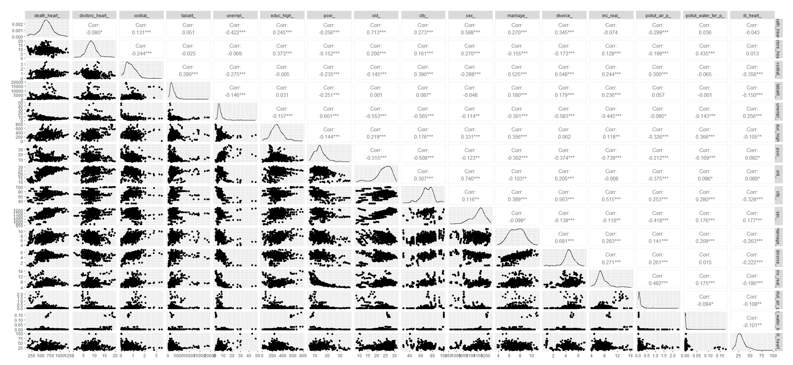
Figure A2.
Correlation matrix and distribution of the dependent variable and the indicator of cardiologists' availability, as well as the considered instrumental variables, taking into account logarithmization.
Figure A2.
Correlation matrix and distribution of the dependent variable and the indicator of cardiologists' availability, as well as the considered instrumental variables, taking into account logarithmization.
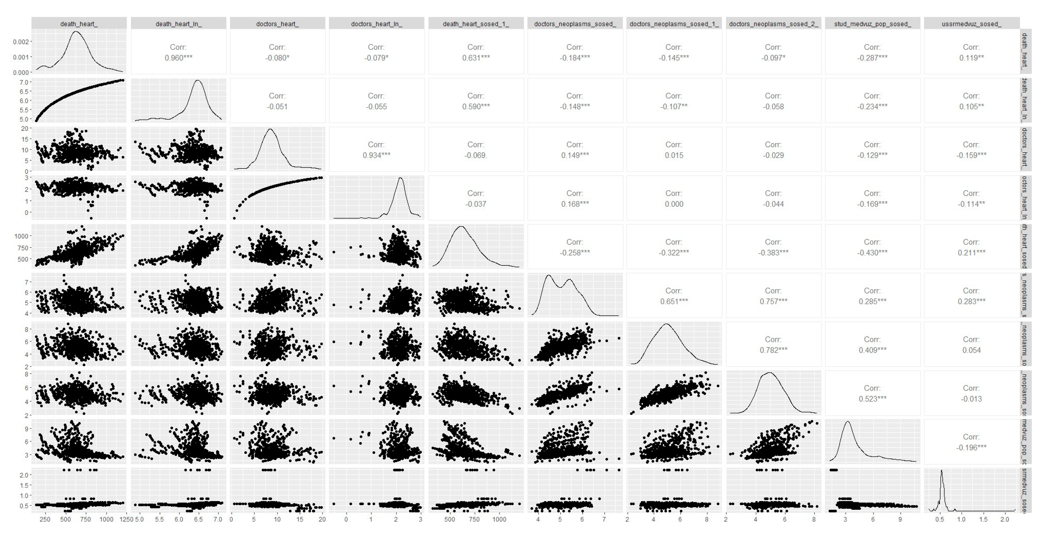
References
- Mosadeghrad, A.M. (2014). Factors influencing healthcare service quality. Int J Health Policy Manag. 3(2), 77-89. [CrossRef]
- Judyth, L. Twigg, (1999), Obligatory medical insurance in Russia: the participants' perspective, Social Science & Medicine. 49, 3, 371-382. [CrossRef]
- Federal Law No. 466-FZ of December 5, 2022 "On the federal budget for 2023 and for the planning period of 2024 and 2025". [Electronic resource]. – Access mode: https://www.consultant.ru/document/cons_doc_LAW_433298/ (accessed on 10.03.2023).
- Winkelmann R. (2004). Health Care Reform and the Number of Doctor Visits: An Econometric Analysis. Journal of Applied Econometrics. 19(4), 455–472. http://www.jstor.org/stable/25146297.
- Bloor K, Hendry V, Maynard A. (2006) Do we need more doctors? JR Soc Med. 99(6), 281-7. [CrossRef]
- Regions of Russia. Socio-economic indicators [Electronic resource]. – Access mode: https://rosstat.gov.ru/folder/210/document/13204 (accessed on 10.03.2023).
- Szymanowski, R. (2014). Health as a Public Good. Dialogue Polityczne. 41-50. [CrossRef]
- Sarbajit Chaudhuri, Jayanta Kumar Dwibedi, Anindya Biswas, (2017), Subsidizing healthcare in the presence of market distortions, Economic Modeling. 64, 539-552. [CrossRef]
- Dadova A.V. & Kil'metova, R.R. (2020). Problems and prospects for the development of compulsory health insurance in Of Russia. Trends in the development of science and education. [CrossRef]
- Samuelson P. (1954) The Pure Theory of Public Expenditure. Journal of Political Economy, no. 56, pp. 496-505.
- Tan, Khee & Duong, Luu. (2016). Measuring Cost of Living for Ordinary Residents in Cities: A New Index. Business and Management Studies. 2. [CrossRef]
- Nagapetyan Arthur Rubikovich, Popov Maxim Alexandrovich, & Petrukhina Anastasia Sergeevna (2021). spatial autoregressive analysis of susceptibility to pulmonary diseases in residents of the Russian Federation. News of the Far Eastern Federal University. Economics and Management. 1 (97), 98-108.
- Nagapetyan A.R., Petrukhina A.S., & Rymareva A.A. (2023). Modeling of tuberculosis incidence rates in the regions of the Russian Federation based on a family of spatial autoregression models. Theory and practice of social development. 1 (179), 59-67.
- Martinez DA, Zhang H, Bastias M, Feijoo F, Hinson J, Martinez R, Dunstan J, Levin S, Prieto D. (2019) Prolonged wait time is associated with increased mortality for Chilean waiting list patients with non-prioritized conditions. BMC Public Health. 19(1), 233. [CrossRef]
- Prentice JC, Pizer SD. (2007) Delayed access to health care and mortality. Health Serv Res. (2007) Apr;42(2):644-62. [CrossRef]
- Birkmeyer JD, Reames BN, McCulloch P, Carr AJ, Campbell WB, Wennberg JE. (2013) Understanding of regional variation in the use of surgery. Lancet. 28;382(9898), 1121-9. [CrossRef]
- Putri LP, O'Sullivan BG, Russell DJ, Kippen R. (2020) Factors associated with increasing rural doctor supply in Asia-Pacific LMICs: a scoping review. Hum Resource Health. 2020 1;18(1):93. [CrossRef]
- Kari JT, Pehkonen J, Hirvensalo M, Yang X, Hutri-Kähönen N, Raitakari OT, Tammelin TH. (2015) Income and Physical Activity among Adults: Evidence from Self-Reported and Pedometer-Based Physical Activity Measurements. PLOS One. 28;10(8):e0135651. [CrossRef]
- Qiu Y, Lu W, Guo J, Sun C, Liu X. (2020) Examining the Urban and Rural Healthcare Progress in Big Cities of China: Analysis of Monitoring Data in Dalian from 2008 to 2017. Int J Environ Res Public Health. 12;17(4):1148. [CrossRef]
- Starfield B, Shi L, Macinko J. (2005) Contribution of primary care to health systems and health. Milbank Q. 83(3), 457-502. [CrossRef]
- Karpina Elena Viktorovna (2022). The impact of lifestyle on human health. E-Scio. 1(64), 578-582.
- Kim ES, Park N, Sun JK, Smith J, Peterson C. (2013) Life satisfaction and frequency of doctor visits. Psychosom Med. 76(1):86-93. [CrossRef]
- Aboumatar HJ, Carson KA, Beach MC, Roter DL, Cooper LA. (2013) The impact of health literacy on desire for participation in healthcare, medical visit communication, and patient reported outcomes among patients with hypertension. JG Intern Med. 28(11):1469-76. [CrossRef]
- Karsten, S. G. (1995). Health Care: Private Good vs. public good. The American Journal of Economics and Sociology. 54, 129-144.
- Horne, L. (2019). Public Health, Public Goods, and Market Failure. Public Health Ethics. 12. 287-292. [CrossRef]
- Lewis, Paul. (2017). Quasi-markets: An Overview and Analysis.
- Fisk, M. (1996). Health care as a public good. Journal of social philosophy. 27(3), 14–40. [CrossRef]
- Anomaly Jonathan. (2011). Public Health and Public Goods.
- Dees Richard. (2018). Public Health and Regulatory Public Goods. Public Health Ethics. [CrossRef]
- Wan EYF, Fung, WT, Schooling, CM, Au Yeung, SL, Kwok, MK, Yu, EYT, Wang, Y., Chan, EWY, Wong, ICK, & Lam, CLK (2021). Blood Pressure and Risk of Cardiovascular Disease in UK Biobank: A Mendelian Randomization Study. Hypertension (Dallas, Tex.: 1979). 77(2), 367–375. [CrossRef]
- Rapsomaniki, E. , Timmis, A., George, J., Pujades-Rodriguez, M., Shah, AD, Denaxas, S., White IR, Caulfield MJ, Deanfield, JE, Smeeth, L., Williams, B., Hingorani, A., & Hemingway, H. (2014). Blood pressure and incidence of twelve cardiovascular diseases: lifetime risks, healthy life-years lost, and age-specific associations in 1 25 million people. Lancet (London, England). 383(9932), 1899-1911. [CrossRef]
- Nordestgaard BG, Palmer, TM, Benn, M., Zacho, J., Tybjaerg-Hansen, A., Davey Smith, G., & Timpson, NJ (2012). The effect of elevated body mass index on ischemic heart disease risk: causal estimates from a Mendelian randomization approach. PLoS medicine. 9(5), e1001212. [CrossRef]
- Larsson SC, Bäck M., Rees, JMB, Mason, AM, & Burgess, S. (2020). Body mass index and body composition in relation to 14 cardiovascular conditions in the UK Biobank: a Mendelian randomization study. European heart journal. 41(2), 221–226. [CrossRef]
- Howard BV, & Magee M.F. (2000). Diabetes and cardiovascular disease. Current atherosclerosis reports. 2(6), 476–481. 6. [CrossRef]
- Stamler, J. , Vaccaro, O., Neaton J.D., & Wentworth, D. (1993). Diabetes, other risk factors, and 12-yr cardiovascular mortality for men screened in the Multiple Risk Factor Intervention Trial. Diabetes care. 16(2), 434–444. [CrossRef]
- Kondo, T. , Nakano Y., Adachi S., & Murohara T. (2019). Effects of Tobacco Smoking on Cardiovascular Disease. Circulation journal : official journal of the Japanese Circulation Society. 83(10), 1980–1985. [CrossRef]
- Larsson SC, Wallin A., & Wolk A. (2018). Alcohol consumption and risk of heart failure: Meta-analysis of 13 prospective studies. Clinical nutrition (Edinburgh, Scotland). 37(4), 1247–1251. [CrossRef]
- van de Luitgaarden IAT, van Oort S., Bouman EJ, Schoonmade LJ, Schrieks IC, Grobbee DE, van der Schouw, YT, Larsson SC, Burgess S., van Ballegooijen, AJ, Onland- Moret, NC, & Beulens JWJ (2022). Alcohol consumption in relation to cardiovascular diseases and mortality: a systematic review of Mendelian randomization studies. European journal of epidemiology. 37(7), 655–669. [CrossRef]
- Hoek, A.G. , van Oort S., Mukamal KJ, & Beulens JWJ (2022). Alcohol Consumption and Cardiovascular Disease Risk: Placing New Data in Context. Current atherosclerosis reports. 24(1), 51–59. [CrossRef]
- Rasmussen JN, Rasmussen, S., Gislason GH, Buch, P., Abildstrom SZ, Køber L., Osler M., Diderichsen F., Torp-Pedersen C., & Madsen M. ( 2006). Mortality after acute myocardial infarction according to income and education. Journal of epidemiology and community health. 60(4), 351–356. [CrossRef]
- Huo X., Khera R., Zhang L., Herrin J., Bai X., Wang Q., Lu Y., Nasir K., Hu S., Li, J., Li X., Zheng X., Masoudi F. A., Spertus J. A., Krumholz H. M., & Jiang L. (2019). Education level and outcomes after acute myocardial infarction in China. Heart (British Cardiac Society). 105(12), 946–952. [CrossRef]
- Hamad, R. , Nguyen TT, Bhattacharya J., Glymour MM, & Rehkopf DH (2019). Educational attainment and cardiovascular disease in the United States: A quasi-experimental instrumental variables analysis. PLoS medicine. 16(6), e1002834. [CrossRef]
- Schultz, WM, Hayek, SS, Samman Tahhan, A., Ko, YA, Sandesara, P., Awad, M., Mohammed, KH, Patel, K., Yuan, M., Zheng, S., Topel, ML, Hartsfield, J., Bhimani, R., Varghese, T., Kim, JH, Shaw, L., Wilson, P., Vaccarino, V., & Quyyumi, A.A. (2017). Marital Status and Outcomes in Patients With Cardiovascular Disease. Journal of the American Heart Association. 6(12), e005890. [CrossRef]
- Gallo, WT, Teng, HM, Falba, TA, Kasl, SV, Krumholz, HM, & Bradley, EH (2006). The impact of late career job loss on myocardial infarction and stroke: a 10 year follow up using the health and retirement survey. Occupational and environmental medicine. 63(10), 683–687. [CrossRef]
- Silverman, A.L. , Herzog, A.A., & Silverman, D.I. (2019). Hearts and Minds: Stress, Anxiety, and Depression: Unsung Risk Factors for Cardiovascular Disease. Cardiology in review. 27(4), 202–207. [CrossRef]
- Kubzansky, LD, Huffman, JC, Boehm, JK, Hernandez, R., Kim, ES, Koga, HK, Feig, EH, Lloyd-Jones, DM, Seligman, MEP, & Labarthe, DR (2018). Positive Psychological Well-Being and Cardiovascular Disease: JACC Health Promotion Series. Journal of the American College of Cardiology. 72(12), 1382–1396. [CrossRef]
- Pope, CA, 3rd, Burnett, RT, Thurston, GD, Thun, MJ, Calle, EE, Krewski, D., & Godleski, JJ (2004). Cardiovascular mortality and long-term exposure to particulate air pollution: epidemiological evidence of general pathophysiological pathways of disease. Circulation. 109(1), 71–77. [CrossRef]
- Hoek G., Brunekreef B., Fischer P., & van Wijnen J. (2001). The association between air pollution and heart failure, arrhythmia, embolism, thrombosis, and other cardiovascular causes of death in a time series study. Epidemiology (Cambridge, Mass.). 12(3), 355–357. 3. [CrossRef]
- Basu, R. , & Samet, JM (2002). Relationship between elevated ambient temperature and mortality: a review of the epidemiologic evidence. Epidemiological reviews. 24(2), 190–202. [CrossRef]
- Kysely, J., Pokorna, L., Kyncl, J., & Kriz, B. (2009). Excess cardiovascular mortality associated with cold spells in the Czech Republic. BMC public health. 9, 19. [CrossRef]
- Humphries, KH, Izadnegahdar, M., Sedlak, T., Saw, J., Johnston, N., Schenck-Gustafsson, K., Shah, RU, Regitz-Zagrosek, V., Grewal, J., Vaccarino, V ., Wei, J., & Bairey Merz, CN (2017). Sex differences in cardiovascular disease - Impact on care and outcomes. Frontiers in neuroendocrinology. 46, 46–70. [CrossRef]
- Groenewegen, KA, den Ruijter, HM, Pasterkamp, G., Polak, JF, Bots, ML, & Peters, SA (2016). Vascular age to determine cardiovascular disease risk: A systematic review of its concepts, definitions, and clinical applications. European journal of preventive cardiology. 23(3), 264–274. [CrossRef]
- Pool, LR, Ning, H., Lloyd-Jones, DM, & Allen, NB (2017). Trends in Racial/Ethnic Disparities in Cardiovascular Health Among US Adults From 1999-2012. Journal of the American Heart Association. 6(9), e006027. [CrossRef]
- Reichel, K. , Prigge, M., Latza, U., Kurth, T., & Backé, E.M. (2022). Association of occupational sitting with cardiovascular outcomes and cardiometabolic risk factors: a systematic review with a sex-sensitive/gender-sensitive perspective. BMJ open. 12(2), e048017. [CrossRef]
- Zhang, N. (2018) Trends in urban/rural inequalities in cardiovascular risk bio-markers among Chinese adolescents in two decades of urbanisation: 1991-2011. International journal for equity in health. 17(1), 101. [CrossRef]
- Simionescu, M. , Bilan S., Gavurova B., & Bordea EN (2019). Health Policies in Romania to Reduce the Mortality Caused by Cardiovascular Diseases. International journal of environmental research and public health. 16(17), 3080. [CrossRef]
- Gavurová Beáta & Toth Peter & Čiutienė Ruta & Tarhaničová Miriam (2019) The impact of healthcare availability on the amenable mortality: Country study. Economics and Sociology. 12.. 236-250. [CrossRef]
- Sundmacher, L. , & Kopetsch T. (2015) The impact of office-based care on hospitalizations for ambulatory care sensitive conditions. The European journal of health economics : HEPAC : health economics in prevention and care. 16(4), 365–375. [CrossRef]
- Sundmacher L., & Busse R. (2011) The impact of physician supply on avoidable cancer deaths in Germany. A spatial analysis. Health policy (Amsterdam, Netherlands). 103(1), 53–62. [CrossRef]
- Dzampe, A.K. , & Takahashi S. (2022) Competition and physician-induced demand in a healthcare market with regulated price: evidence from Ghana. International journal of health economics and management. 22(3), 295–313. [CrossRef]
- Farahani Mansoor & Subramanian S. & Canning David. (2009). Short and long-term relationship between physician density on infant mortality: a longitudinal econometric analysis.
- The Australian Institute of Health and Welfare is Australia's national health and welfare statistics and information agency. (2005) The health of australia's workforce.
- Dizon-Ross R, Dupas P, Robinson J. (2017) Governance and the effectiveness of public health subsidies: Evidence from Ghana, Kenya and Uganda. J Public Economy. 156,150-169. [CrossRef]
- Velieva, F.E. (2019) Features of the development of the system of compulsory and voluntary health insurance. Economics and Society. (1-1 (56)), 126-128.
- Qinan Wang, (2004) Modeling and analysis of high risk patient queues, European Journal of Operational Research. 155(2), 502-515. [CrossRef]
- Tulchinsky, T.H. (2018) Bismarck and the Long Road to Universal Health Coverage. Case Studies in Public Health. 131–79. [CrossRef]
- Sargan, JD (1958) "The Estimation of Economic Relationships Using Instrumental Variables". Econometrics. 26(3), 393-415. [CrossRef]
- DA Griffith, (2009) Spatially Autoregressive Models, International Encyclopedia of Human Geography, Elsevier, Pages 396-402. [CrossRef]
- Bo Sun, Bo Wang (2021) Spatial Spillover Effects of Air Pollution on the Health Expenditure of Rural Residents: Based on Spatial Durbin Model. Int. J. Environ. Res. Public Health. 18(13), 7058. [CrossRef]
- Latimaha Rusli & Bahari Zakaria & Ismail Nor Asmat (2020) Cost of Living and Standard of Living Nexus: The Determinants of Cost of Living. Jurnal Ekonomi Malaysia. 54, 1-14. [CrossRef]

Table 1.
Description of variables.
| No. | Designation | Factor | Calculation method |
|---|---|---|---|
| 1 | death_heart_ | Mortality from CVD | Mortality from diseases of the circulatory system (per 100 thousand population) |
| 2 | doctors_heart_ | Number of cardiologists | Number of cardiologists per 100,000 people |
| 3 | vodkat_ | Alcohol consumption | alcohol consumption,dl/person |
| 4 | tabakt_ | Tobacco consumption | Consumption of tobacco products (sales), rub. per person |
| 5 | unempl_ | Unemployment | Unemployment rate (according to sample labor force surveys; in percent) |
| 6 | educ_high_ | Higher education | Estimation of the share of the population with higher education in the region (number of students enrolled in bachelor's, specialist's, master's programs per 10,000 population) |
| 7 | poor_ | Poverty rate | Proportion of the poor (income below the subsistence level) |
| 8 | old_ | Proportion of the elderly | Share of people older than working age |
| 9 | city_ | Percentage of urban population | Share of the urban population in the total population, in percent |
| 10 | sex_ | Male to female ratio | There are women per 1000 men |
| eleven | marriage_ | Marriage | General marriage rates per 1000 population |
| 12 | divorce_ | Divorceability | General divorce rates per 1000 population |
| 13 | inc_real_ | Real per capita income | Nominal income divided by the cost of a fixed set of consumer goods and services |
| 14 | pollut_air_p_ | Air pollution | Pollutant emissions, thousand tons per person |
| 15 | pollut_water_ter_p_ | Water pollution | Emissions of pollutants, thousand cubic meters meters per sq.m. for 1 person) |
| 16 | ill_heart_ | CVD incidence rate | Diseases of the circulatory system, number, registered diseases per 1000 population |
| 17 | death_heart_sated_1_ | Average CVD mortality in neighboring regions (nearest neighbors) | Average mortality rate from CVD in neighboring regions that have a common border with the region under consideration |
| 18 | doctors_neoplasms_sosed_ | The average level of provision with oncologists in neighboring regions (neighbors - all other regions of the Russian Federation) | Average weighted level of provision with oncologists in neighboring regions based on the matrix of squared inverse distances (more details in subsection 3.5) |
| 19 | doctors_neoplasms_sosed_1_ | Average level of provision with oncologists in neighboring regions (nearest neighbors) | The average level of provision with oncologists in neighboring regions that have a common border with the region under consideration (more details in subsection 3.5) |
| 20 | doctors_neoplasms_sosed_2_ | Average level of provision with oncologists in neighboring regions (nearest neighbors and their neighbors) | The average level of provision with oncologists in neighboring regions that have a common border with the region under consideration or a common border with a region that has a common border with the region under consideration (more details in subsection 3.5) |
| 21 | stud_medvuz_pop_sated_ | The average level of provision with medical students in neighboring regions (neighbors - all other regions of the Russian Federation) | The average level of provision with medical students (the number of students studying in medical specialties per 1000 population) in neighboring regions based on the matrix of squared inverse distances (more details in subsection 3.5) |
| 22 | ussrmedvuz_sosed_ | The average level of provision with medical institutions in neighboring regions in 1991 (neighbors - all other regions of the Russian Federation) | The average level of provision with medical institutions (presence or absence of a medical school) in neighboring regions in 1991 based on the matrix of squared inverse distances (more details in subsection 3.5) |
Table 2.
Statistical properties considered data.
| Variable | Mean | Std. Dev. | Min | Max |
|---|---|---|---|---|
| death_heart_ | 629.73 | 184.91 | 131.20 | 1204.70 |
| doctors_heart_ | 8.87 | 2.73 | 0.59 | 19.72 |
| vodkat_ | 0.79 | 0.45 | 0 | 3.44 |
| tabakt_ | 2401.93 | 2249.27 | 40.09 | 19119.94 |
| unempl_ | 6.49 | 4.22 | 0.80 | 47.70 |
| educ_high_ | 284.80 | 117.96 | 0 | 786.00 |
| poor_ | 14.25 | 5.01 | 5.60 | 37.80 |
| old_ | 23.60 | 4.81 | 8.30 | 31.30 |
| city_ | 70.16 | 13.01 | 28.90 | 100.00 |
| sex_ | 1144.93 | 53.43 | 961.00 | 1236.00 |
| marriage_ | 7.28 | 1.34 | 3.80 | 11.10 |
| divorce_ | 4.39 | 1.03 | 0.50 | 7.00 |
| inc_real_ | 7.29 | 1.89 | 3.87 | 16.41 |
| pollut_air_p_ | 0.17 | 0.29 | 0.0005 | 2.34 |
| pollut_water_ter_p_ | 0.00 | 0.02 | 0 | 0.17 |
| ill_heart_ | 31.27 | 10.58 | 11.90 | 98.40 |
| death_heart_sosed_1_ | 646.89 | 139.14 | 323.68 | 1204.70 |
| doctors_neoplasms_sosed_ | 5.0729 | 0.63 | 3.71 | 7.65 |
| doctors_neoplasms_sosed_1_ | 5.0734 | 1.07 | 2.28 | 8.83 |
| doctors_neoplasms_sosed_2_ | 5.03 | 0.82 | 2.28 | 8.17 |
| stud_medvuz_pop_sosed_ | 4.08 | 1.75 | 1.23 | 10.71 |
| ussrmedvuz_sosed_ | 0.57 | 0.20 | 0.24 | 2.23 |
Table 3.
Results of evaluation of the considered linear models.
| Pooled Models | Panel Models with FE | ||||||
|---|---|---|---|---|---|---|---|
| No IV | IV: doctors_neoplasms_sosed_ | IV: stud_medvuz_pop_sosed_ | IV: ussrmedvuz_sosed__ | IV: doctors_neoplasms_sosed_, stud_medvuz_pop_sosed_, ussrmedvuz_sosed_ | No IV | IV: stud_medvuz_pop_sosed_ | |
| VARIABLES | m1.1 | m1.2 | m1.3 | m1.4 | m1.5 | m1.6 | m1.7 |
| Number of cardiologists | -11.240*** | -58.285*** | -43.827*** | -25.316 | -48.166*** | -7.477** | -45.973*** |
| (1.946) | (16.358) | (15.329) | (22.840) | (9.559) | (3.291) | (11.665) | |
| Alcohol consumption | 43.612*** | 12.868 | 22.316 | 34.413* | 19.481 | 7.954 | 22.763 |
| (11.416) | (21.560) | (16.367) | (18.110) | (16.837) | (11.586) | (17.515) | |
| Tobacco consumption | -0.001 | -0.000 | -0.000 | -0.001 | -0.000 | 0.002 | -0.001 |
| (0.002) | (0.002) | (0.002) | (0.002) | (0.002) | (0.003) | (0.002) | |
| Unemployment _ | 2.199 | 2.218 | 2.212 | 2.205 | 2.214 | -2.351 | -4.085** |
| (1.776) | (2.668) | (2.293) | (1.918) | (2.400) | (1.529) | (1.767) | |
| Higher education | 0.008 | 0.376** | 0.263** | 0.118 | 0.297*** | 0.264** | 0.265** |
| (0.045) | (0.150) | (0.127) | (0.177) | (0.102) | (0.104) | (0.110) | |
| Poverty rate | -5.065*** | -8.603*** | -7.516*** | -6.124*** | -7.842*** | -0.293 | 1.633 |
| (1.349) | (2.501) | (1.918) | (2.098) | (2.003) | (2.011) | (1.769) | |
| Proportion of the elderly | 26.495*** | 20.183*** | 22.123*** | 24.607*** | 21.541*** | -22.88*** | -9.491 |
| (2.516) | (3.651) | (3.067) | (3.901) | (2.959) | (6.422) | (7.112) | |
| Percentage of urban population | -0.203 | 1.431* | 0.929 | 0.286 | 1.079* | 3.413 | 6.783** |
| (0.453) | (0.849) | (0.711) | (0.902) | (0.637) | (3.600) | (3.383) | |
| Male to female ratio | 0.570*** | 0.900*** | 0.799*** | 0.669*** | 0.829*** | 3.436*** | 3.226*** |
| (0.165) | (0.214) | (0.196) | (0.228) | (0.182) | (0.865) | (0.646) | |
| Marriage | 48.762*** | 1.987 | 16.362 | 34.767 | 12.048 | 5.020 | -11.313* |
| (5.946) | (17.448) | (15.589) | (23.280) | (11.388) | (4.552) | (6.813) | |
| Divorceability | -12.705 | 3.910 | -1.196 | -7.734 | 0.336 | -7.374 | 5.222 |
| (8.606) | (11.763) | (11.013) | (11.818) | (10.372) | (8.275) | (11.181) | |
| Real per capita income | -21.129*** | -18.296*** | -19.166*** | -20.281*** | -18.905*** | -0.633 | 18.853** |
| (3.755) | (5.366) | (4.760) | (4.391) | (4.791) | (10.508) | (9.395) | |
| Air pollution | 4.523 | -45.775* | -30.318 | -10.527 | -34.956* | -43.527 | -32.238 |
| (17.020) | (25.659) | (23.192) | (31.548) | (19.489) | (41.265) | (37.038) | |
| Water pollution | -401.544* | 2,097.79** | 1,329.704 | 346.291 | 1,560.2*** | 357.700 | 1,216.451 |
| (205.871) | (916.763) | (841.021) | (1,223.388) | (557.358) | (585.244) | (1,107.782) | |
| CVD incidence rate | -1.155*** | -1.120* | -1.131** | -1.144*** | -1.127** | -1.089* | -0.906* |
| (0.409) | (0.581) | (0.500) | (0.427) | (0.522) | (0.590) | (0.480) | |
| Constant | -619.4*** | -332.711 | -420.828** | -533.7*** | -394.386** | -2,964** | |
| (149.004) | (223.260) | (186.167) | (197.203) | (188.891) | (1,164) | ||
| Observations | 664 | 664 | 664 | 664 | 664 | 664 | 664 |
| AIC | 8019 | 8478 | 8278 | 8076 | 8337 | 6998 | 7233 |
| BIC | 8091 | 8550 | 8350 | 8148 | 8409 | 7065 | 7301 |
| Number of region | 83 | 83 | |||||
Robust standard errors in parentheses. *** p<0.01, ** p<0.05, * p<0.1
Table 4.
Results of evaluation of the considered nonlinear models using the logarithm.
| Pooled Models | Panel Models with FE | ||||||
|---|---|---|---|---|---|---|---|
| No IV | IV: doctors_neoplasms_sosed_ | IV: stud_medvuz_pop_sosed_ | IV: ussrmedvuz_sosed__ | IV: doctors_neoplasms_sosed_, stud_medvuz_pop_sosed_, ussrmedvuz_sosed_ | No IV | IV: stud_medvuz_pop_sosed_ | |
| VARIABLES | m2.1 | m2.2 | m2.3 | m2.4 | m2.5 | m2.6 | m2.7 |
| Number of cardiologists (logarithm) | -0.164*** | -0.724*** | -0.557** | -0.603* | -0.704*** | -0.064 | -0.648*** |
| (0.022) | (0.182) | (0.271) | (0.342) | (0.138) | (0.041) | (0.163) | |
| Alcohol consumption | 0.083*** | 0.025 | 0.042 | 0.037 | 0.027 | 0.000 | 0.012 |
| (0.020) | (0.035) | (0.035) | (0.043) | (0.033) | (0.019) | (0.027) | |
| Tobacco consumption | 0.000 | 0.000 | 0.000 | 0.000 | 0.000 | 0.000 | 0.000 |
| (0.000) | (0.000) | (0.000) | (0.000) | (0.000) | (0.000) | (0.000) | |
| Unemployment _ | -0.001 | -0.003 | -0.002 | -0.002 | -0.003 | 0.002 | -0.003 |
| (0.003) | (0.004) | (0.004) | (0.004) | (0.004) | (0.003) | (0.004) | |
| Higher education | 0.000*** | 0.001*** | 0.001** | 0.001* | 0.001*** | 0.000** | 0.000* |
| (0.000) | (0.000) | (0.000) | (0.000) | (0.000) | (0.000) | (0.000) | |
| Poverty rate | -0.007*** | -0.015*** | -0.013*** | -0.013** | -0.015*** | -0.006** | -0.003 |
| (0.003) | (0.005) | (0.005) | (0.006) | (0.004) | (0.003) | (0.003) | |
| Proportion of the elderly | 0.060*** | 0.050*** | 0.053*** | 0.052*** | 0.050*** | -0.042*** | -0.014 |
| (0.005) | (0.006) | (0.007) | (0.007) | (0.006) | (0.010) | (0.013) | |
| Percentage of urban population | -0.001 | 0.002 | 0.001 | 0.001 | 0.002* | 0.002 | 0.008 |
| (0.001) | (0.001) | (0.002) | (0.002) | (0.001) | (0.005) | (0.005) | |
| Male to female ratio | 0.000 | 0.001** | 0.001 | 0.001 | 0.001** | 0.005*** | 0.006*** |
| (0.000) | (0.000) | (0.000) | (0.000) | (0.000) | (0.001) | (0.001) | |
| Marriage | 0.085*** | 0.026 | 0.043 | 0.038 | 0.028 | 0.009 | -0.013 |
| (0.009) | (0.023) | (0.029) | (0.038) | (0.019) | (0.006) | (0.011) | |
| Divorceability | -0.014 | -0.005 | -0.008 | -0.007 | -0.005 | -0.012 | -0.007 |
| (0.015) | (0.022) | (0.018) | (0.020) | (0.021) | (0.013) | (0.020) | |
| Real per capita income | -0.045*** | -0.046*** | -0.046*** | -0.046*** | -0.046*** | -0.019 | 0.011 |
| (0.007) | (0.008) | (0.007) | (0.008) | (0.008) | (0.021) | (0.015) | |
| Air pollution | 0.022 | -0.050 | -0.028 | -0.034 | -0.047 | -0.037 | -0.003 |
| (0.035) | (0.043) | (0.045) | (0.055) | (0.039) | (0.059) | (0.060) | |
| Water pollution | -0.903*** | 0.999 | 0.432 | 0.586 | 0.930 | 0.959 | 2.614** |
| (0.293) | (0.743) | (0.953) | (1.185) | (0.604) | (0.716) | (1.187) | |
| CVD incidence rate | -0.002** | -0.001 | -0.001 | -0.001 | -0.001 | -0.001 | -0.000 |
| (0.001) | (0.001) | (0.001) | (0.001) | (0.001) | (0.001) | (0.001) | |
| Constant | 4.954*** | 5.875*** | 5.600*** | 5.675*** | 5.841*** | 1.852 | |
| (0.299) | (0.450) | (0.518) | (0.641) | (0.406) | (1.751) | ||
| Observations | 664 | 664 | 664 | 664 | 664 | 664 | 664 |
| AIC | -496.6 | -62.80 | -248.1 | -199.3 | -86.10 | -1596 | -1233 |
| BIC | -424.6 | 9.200 | -176.1 | -127.3 | -14.10 | -1529 | -1165 |
| Number of region | 83 | 83 | |||||
Robust standard errors in parentheses. *** p<0.01, ** p<0.05, * p<0.1.
Table 5.
Results of the evaluation of the considered nonlinear models using the square of the variable characterizing the level of staffing.
Table 5.
Results of the evaluation of the considered nonlinear models using the square of the variable characterizing the level of staffing.
| Pooled Models | Panel Models with FE | ||||||||
|---|---|---|---|---|---|---|---|---|---|
| No IV | IV: doctors_neoplasms_sosed_ | IV: stud_medvuz_pop_sosed_ | IV: ussrmedvuz_sosed__ | IV: doctors_neoplasms_sosed_, stud_medvuz_pop_sosed_, ussrmedvuz_sosed_ | No IV | IV: stud_medvuz_pop_sosed_ | IV: stud_medvuz_pop_sosed_, stud_medvuz_pop_sosed_1_, stud_medvuz_pop_sosed_2 | ||
| VARIABLES | m3.1 | m3.2 | m3.3 | m3.4 | m3.5 | m3.6 | m3.7 | m3.8 | |
| Number of cardiologists | -43.948*** | -138.349* | -165.707*** | -118.737* | -134.193*** | 7.237 | -144.580* | -101.272 | |
| (6.054) | (76.627) | (39.067) | (65.140) | (38.319) | (8.651) | (79.346) | (61.590) | ||
| Number of cardiologists squared | 1.720*** | 5.386 | 6.907*** | 4.199 | 5.134*** | -0.712* | 5.505 | 3.177 | |
| (0.297) | (4.494) | (1.952) | (3.775) | (1.925) | (0.390) | (4.392) | (3.382) | ||
| Alcohol consumption | 37.038*** | 6.890 | 2.107 | 9.499 | 7.441 | 10.792 | -4.975 | 6.134 | |
| (11.201) | (17.904) | (15.761) | (17.730) | (15.942) | (11.916) | (29.778) | (24.615) | ||
| Tobacco consumption | -0.000 | 0.002 | 0.002 | 0.001 | 0.002 | 0.002 | -0.000 | -0.000 | |
| (0.002) | (0.002) | (0.002) | (0.002) | (0.002) | (0.003) | (0.002) | (0.002) | ||
| Unemployment _ | 1.345 | -0.466 | -1.223 | 0.124 | -0.341 | -1.841 | -7.346** | -5.895** | |
| (1.747) | (3.197) | (2.421) | (2.917) | (2.344) | (1.562) | (3.338) | (2.778) | ||
| Higher education | -0.020 | 0.113 | 0.076 | 0.156 | 0.122* | 0.264** | 0.269** | 0.267** | |
| (0.045) | (0.171) | (0.075) | (0.141) | (0.068) | (0.102) | (0.126) | (0.116) | ||
| Poverty rate | -6.040*** | -9.975*** | -10.718*** | -9.524*** | -9.879*** | 0.003 | -1.403 | -0.200 | |
| (1.276) | (2.606) | (2.196) | (2.433) | (2.056) | (1.972) | (3.315) | (2.746) | ||
| Proportion of the elderly | 25.756*** | 20.865*** | 20.422*** | 20.980*** | 20.889*** | -24.394*** | -3.018 | -6.315 | |
| (2.489) | (3.044) | (3.101) | (3.012) | (2.965) | (6.646) | (9.055) | (7.952) | ||
| Percentage of urban population | -0.007 | 1.270* | 1.388** | 1.236* | 1.263** | 3.431 | 5.325 | 5.801* | |
| (0.463) | (0.659) | (0.672) | (0.646) | (0.635) | (3.580) | (3.701) | (3.460) | ||
| Male to female ratio | 0.672*** | 1.064*** | 1.143*** | 1.014*** | 1.053*** | 3.308*** | 4.297*** | 3.853*** | |
| (0.165) | (0.277) | (0.224) | (0.253) | (0.210) | (0.869) | (1.141) | (0.968) | ||
| Marriage | 50.351*** | 29.183* | 32.161*** | 25.159* | 28.326*** | 4.525 | -1.085 | -4.726 | |
| (5.886) | (17.521) | (9.077) | (14.716) | (8.367) | (4.553) | (11.787) | (9.563) | ||
| Divorceability | -15.529* | -12.824 | -15.881 | -9.837 | -12.189 | -5.883 | -11.240 | -4.806 | |
| (8.564) | (15.391) | (11.411) | (13.303) | (10.527) | (8.321) | (17.704) | (14.503) | ||
| Real per capita income | -23.553*** | -27.231*** | -29.471*** | -25.382*** | -26.839*** | 0.367 | 3.488 | 9.170 | |
| (3.541) | (8.316) | (4.992) | (7.250) | (4.718) | (10.421) | (16.773) | (13.510) | ||
| Air pollution | 1.567 | -31.135 | -32.060 | -32.246* | -31.374* | -44.614 | -28.266 | -30.418 | |
| (16.393) | (20.010) | (20.659) | (19.092) | (18.853) | (41.202) | (43.194) | (37.749) | ||
| Water pollution | -1,289.8*** | -1,870.618 | -2,740.49** | -1,101.606 | -1,707.327* | 234.476 | 1,831.983 | 1,535.75 | |
| (222.212) | (2,874.492) | (1,069.974) | (2,389.143) | (995.426) | (631.838) | (2,036.41) | (1,087.8) | ||
| CVD incidence rate | -0.922** | -0.407 | -0.201 | -0.565 | -0.440 | -1.158* | -0.450 | -0.650 | |
| (0.407) | (0.773) | (0.558) | (0.684) | (0.536) | (0.587) | (0.682) | (0.603) | ||
| Constant | -544.969*** | -235.739 | -179.485 | -269.151 | -242.805 | -2,869.12** | |||
| (146.947) | (213.257) | (187.345) | (207.218) | (188.606) | (1,164.101) | ||||
| Observations | 664 | 664 | 664 | 664 | 664 | 664 | 664 | 664 | |
| AIC | 7998 | 8244 | 8302 | 8236 | 8241 | 6994 | 7400 | 7262 | |
| BIC | 8074 | 8321 | 8379 | 8312 | 8317 | 7066 | 7472 | 7334 | |
| Number of region | 83 | 83 | 83 | ||||||
Robust standard errors in parentheses. *** p<0.01, ** p<0.05, * p<0.1
Table 6.
Results of the evaluation of the considered nonlinear models using the square of the variable characterizing the level of staffing.
Table 6.
Results of the evaluation of the considered nonlinear models using the square of the variable characterizing the level of staffing.
| Pooled Models | Spatial AR Panel Models with FE | |||||
|---|---|---|---|---|---|---|
| IV: doctors_neoplasms_sosed_ | IV: doctors_neoplasms_sosed | IV: doctors_neoplasms_sosed | IV: doctors_neoplasms_sosed | Spatial Avtoregressive | Spatial Darbin | |
| VARIABLES | m1.2 | m4.1 | m4.2 | m4.3 | m4.4 | m4.5 |
| -58.285*** | -56.667*** | -57.140*** | -51.783*** | -6.502** | -4.262 | |
| Number of cardiologists | (16.358) | (16.559) | (15.327) | (18.682) | (3.230) | (2.713) |
| 12.868 | 8.147 | 14.095 | 8.905 | -20.984** | -30.974* | |
| Alcohol consumption | (21.560) | (21.372) | (20.216) | (19.166) | (10.701) | (16.767) |
| -0.000 | -0.000 | -0.000 | -0.000 | 0.002 | 0.001 | |
| Tobacco consumption | (0.002) | (0.002) | (0.002) | (0.002) | (0.003) | (0.002) |
| 2.218 | -7.131*** | 2.145 | 2.223 | -3.320*** | -3.924*** | |
| Unemployment _ | (2.668) | (2.326) | (2.569) | (2.526) | (1.071) | (1.257) |
| 0.376** | 0.378** | 0.365*** | 0.342** | 0.037 | -0.073 | |
| Higher education | (0.150) | (0.150) | (0.138) | (0.157) | (0.066) | (0.067) |
| -8.603*** | -9.934*** | -8.503*** | -7.858*** | -1.045 | -0.507 | |
| Poverty rate | (2.501) | (2.354) | (2.422) | (2.672) | (1.782) | (1.513) |
| 20.183*** | 20.764*** | 19.964*** | 0.044 | 25.843*** | ||
| Proportion of the elderly | (3.651) | (3.341) | (3.392) | (5.168) | (8.979) | |
| 1.431* | 1.636* | 1.453* | 1.379* | 3.813 | 0.656 | |
| Percentage of urban population | (0.849) | (0.853) | (0.846) | (0.814) | (2.824) | (2.800) |
| 0.900*** | 1.982*** | 0.864*** | 0.774*** | 2.261*** | 1.651** | |
| Male to female ratio | (0.214) | (0.131) | (0.198) | (0.245) | (0.737) | (0.785) |
| 1.987 | -22.886 | 4.844 | 4.711 | 2.048 | 10.669 | |
| Marriage | (17.448) | (14.849) | (14.278) | (17.594) | (3.890) | (6.554) |
| 3.910 | 36.117*** | 2.390 | 1.130 | -0.657 | ||
| Divorceability | (11.763) | (11.039) | (11.091) | (7.428) | (9.265) | |
| -18.296*** | -22.803*** | -18.675*** | -18.598*** | -3.399 | -8.792 | |
| Real per capita income | (5.366) | (5.525) | (5.206) | (4.820) | (9.522) | (7.992) |
| -45.775* | -100.928*** | -42.395* | -32.041 | -38.340 | -39.453 | |
| Air pollution | (25.659) | (26.144) | (23.803) | (28.713) | (33.380) | (27.904) |
| 2,097.786** | 1,874.074** | 2,018.6** | 1,781.924* | -1,452*** | -1,574.936*** | |
| Water pollution | (916.763) | (936.554) | (853.735) | (1,020.319) | (376.600) | (556.820) |
| -1.120* | -0.744 | -1.100* | -0.928 | -0.464 | -0.075 | |
| CVD incidence rate | (0.581) | (0.576) | (0.568) | (0.571) | (0.508) | (0.452) |
| Average CVD mortality in neighboring regions (nearest neighbors) | 0.103 | |||||
| (0.080) | ||||||
| Spatial rho | 0.782*** | -0.146 | ||||
| (0.063) | (0.114) | |||||
| SPATIAL X | + | |||||
| Observations | 664 | 664 | 664 | 664 | 664 | 664 |
| AIC | 8478 | 8493 | 8460 | 8384 | 6900 | 6756 |
| BIC | 8550 | 8560 | 8527 | 8461 | 6977 | 6900 |
| Number of region | 83 | 83 | 83 | 83 | 83 | 83 |
Robust standard errors in parentheses. *** p<0.01, ** p<0.05, * p<0.1
Table 7.
Results of evaluation of the considered models for Robustness Check 2.
| Pooled Models | Panel Models with FE | |||||||||
|---|---|---|---|---|---|---|---|---|---|---|
| IV: doctors_neoplasms_sosed_ | IV: doctors_neoplasms_sosed_1_ | IV: doctors_neoplasms_sosed_2_ | IV: doctors_neoplasms_sosed_, ussrmedvuz_sosed_ | IV: doctors_neoplasms_sosed_1_, ussrmedvuz_sosed_ | IV: doctors_neoplasms_sosed_2_, ussrmedvuz_sosed_ | IV: doctors_neoplasms_sosed_ | IV: doctors_neoplasms_sosed_1_ | IV: doctors_neoplasms_sosed_2_ | IV: stud_medvuz_pop_sosed_, stud_medvuz_pop_sosed_1_, stud_medvuz_pop_sosed_2 | |
| VARIABLES | m2.2 | m5.1 | m5.2 | m5.3 | m5.4 | m5.5 | m2.7 | m5.6 | m5.7 | m5.8 |
| Number of cardiologists (logarithm) | -0.724*** | 1.798 | 0.456 | -0.697*** | -0.360 | -0.232 | -0.648*** | -0.932*** | -0.713*** | -0.618*** |
| (0.182) | (3.209) | (0.712) | (0.135) | (0.337) | (0.274) | (0.163) | (0.273) | (0.182) | (0.157) | |
| Alcohol consumption | 0.025 | 0.288 | 0.148** | 0.028 | 0.063 | 0.076** | 0.012 | 0.017 | 0.013 | 0.011 |
| (0.035) | (0.310) | (0.074) | (0.032) | (0.039) | (0.033) | (0.027) | (0.034) | (0.029) | (0.026) | |
| Tobacco consumption | 0.000 | -0.000 | -0.000 | 0.000 | 0.000 | 0.000 | 0.000 | -0.000 | 0.000 | 0.000 |
| (0.000) | (0.000) | (0.000) | (0.000) | (0.000) | (0.000) | (0.000) | (0.000) | (0.000) | (0.000) | |
| Unemployment _ | -0.003 | 0.006 | 0.001 | -0.003 | -0.002 | -0.001 | -0.003 | -0.006 | -0.004 | -0.003 |
| (0.004) | (0.014) | (0.005) | (0.004) | (0.004) | (0.003) | (0.004) | (0.005) | (0.004) | (0.004) | |
| Higher education | 0.001*** | -0.001 | -0.000 | 0.001*** | 0.000 | 0.000 | 0.000* | 0.000 | 0.000* | 0.000* |
| (0.000) | (0.003) | (0.001) | (0.000) | (0.000) | (0.000) | (0.000) | (0.000) | (0.000) | (0.000) | |
| Poverty rate | -0.015*** | 0.022 | 0.002 | -0.015*** | -0.010* | -0.008* | -0.003 | -0.001 | -0.002 | -0.003 |
| (0.005) | (0.045) | (0.010) | (0.004) | (0.005) | (0.005) | (0.003) | (0.004) | (0.003) | (0.003) | |
| Proportion of the elderly | 0.050*** | 0.095 | 0.071*** | 0.050*** | 0.056*** | 0.059*** | -0.014 | -0.000 | -0.011 | -0.015 |
| (0.006) | (0.060) | (0.014) | (0.006) | (0.007) | (0.007) | (0.013) | (0.018) | (0.013) | (0.012) | |
| Percentage of urban population | 0.002 | -0.011 | -0.004 | 0.002* | 0.000 | -0.000 | 0.008 | 0.011* | 0.008 | 0.007 |
| (0.001) | (0.016) | (0.004) | (0.001) | (0.002) | (0.002) | (0.005) | (0.006) | (0.005) | (0.005) | |
| Male to female ratio | 0.001** | -0.002 | -0.001 | 0.001** | 0.000 | 0.000 | 0.006*** | 0.006*** | 0.006*** | 0.006*** |
| (0.000) | (0.004) | (0.001) | (0.000) | (0.000) | (0.000) | (0.001) | (0.001) | (0.001) | (0.001) | |
| Marriage | 0.026 | 0.292 | 0.150* | 0.028 | 0.064* | 0.078*** | -0.013 | -0.024 | -0.016 | -0.012 |
| (0.023) | (0.344) | (0.079) | (0.019) | (0.036) | (0.030) | (0.011) | (0.016) | (0.012) | (0.011) | |
| Divorceability | -0.005 | -0.046 | -0.024 | -0.005 | -0.011 | -0.013 | -0.007 | -0.004 | -0.006 | -0.007 |
| (0.022) | (0.083) | (0.028) | (0.021) | (0.017) | (0.016) | (0.020) | (0.026) | (0.021) | (0.019) | |
| Real per capita income | -0.046*** | -0.040** | -0.043*** | -0.046*** | -0.045*** | -0.045*** | 0.011 | 0.026 | 0.015 | 0.010 |
| (0.008) | (0.020) | (0.009) | (0.008) | (0.007) | (0.007) | (0.015) | (0.020) | (0.015) | (0.014) | |
| Air pollution | -0.050 | 0.272 | 0.101 | -0.046 | -0.003 | 0.013 | -0.003 | 0.013 | 0.001 | -0.005 |
| (0.043) | (0.452) | (0.116) | (0.039) | (0.057) | (0.053) | (0.060) | (0.082) | (0.064) | (0.059) | |
| Water pollution | 0.999 | -7.558 | -3.007 | 0.907 | -0.238 | -0.672 | 2.614** | 3.419** | 2.799** | 2.529** |
| (0.743) | (11.241) | (2.558) | (0.591) | (1.167) | (0.957) | (1.187) | (1.589) | (1.261) | (1.155) | |
| CVD incidence rate | -0.001 | -0.004 | -0.003** | -0.001 | -0.001* | -0.002** | -0.000 | 0.000 | -0.000 | -0.000 |
| (0.001) | (0.005) | (0.001) | (0.001) | (0.001) | (0.001) | (0.001) | (0.001) | (0.001) | (0.001) | |
| Constant | 5.875*** | 1.733 | 3.936*** | 5.830*** | 5.276*** | 5.066*** | ||||
| (0.450) | (5.183) | (1.167) | (0.401) | (0.603) | (0.517) | |||||
| Observations | 664 | 664 | 664 | 664 | 664 | 664 | 664 | 664 | 664 | 664 |
| AIC | -62.80 | 1169 | 5.100 | -93.60 | -425.8 | -487.6 | -1233 | -959.4 | -1170 | -1261 |
| BIC | 9.200 | 1241 | 77.10 | -21.60 | -353.8 | -415.7 | -1165 | -891.9 | -1102 | -1194 |
| Number of region | 83 | 83 | 83 | 83 | 83 | 83 | 83 | 83 | 83 | 83 |
Robust standard errors in parentheses. *** p<0.01, ** p<0.05, * p<0.1
Disclaimer/Publisher’s Note: The statements, opinions and data contained in all publications are solely those of the individual author(s) and contributor(s) and not of MDPI and/or the editor(s). MDPI and/or the editor(s) disclaim responsibility for any injury to people or property resulting from any ideas, methods, instructions or products referred to in the content. |
© 2023 by the authors. Licensee MDPI, Basel, Switzerland. This article is an open access article distributed under the terms and conditions of the Creative Commons Attribution (CC BY) license (http://creativecommons.org/licenses/by/4.0/).
Copyright: This open access article is published under a Creative Commons CC BY 4.0 license, which permit the free download, distribution, and reuse, provided that the author and preprint are cited in any reuse.


