
Submitted:
13 September 2023
Posted:
14 September 2023
You are already at the latest version
Abstract
This paper reports modelling outcomes for improvements to building energy performance in Indonesia. Long-term climate effects due to building energy demands including carbon emissions are also considered. The global change assessment model (GCAM) was used to generate the related end-user building energy data, including socioeconomics for urban areas of Indonesia. As a comprehensive study, the total life cycle of carbon in the building sector and the concept of zero-carbon buildings, including energy efficiency, zero-emissions electricity and fuel switching options were considered. Building shell conductance (u-value) of building envelope, floor area ratio (FAR), air conditioner (AC) efficiency, electrical appliances (APLs) efficiency, rooftop photovoltaic (PV) performance and ground source heat pump (GSHP) systems were considered as parameters to mitigate carbon emissions under the operational energy category in GCAM. Carbon mitigation associated with the cement production process was considered in the raw material category. Urban population and labour productivity in Indonesia were used as base inputs with projected growth rates to 2050 determined from available literature. Low growth rate ‘LowRate’ and high growth rate ‘HighRate’ were considered as variable inputs for u-value, FAR, AC efficiency, APLs efficiency, and PV capacity factor to model emissions mitigation. The energy consumption of the GSHP was compared to the conventional reverse cycle ACs to identify the potential of the GSHP as a fuel-switching option. Only base input data were used for cement production process parameters without applying any variable inputs. GCAM base scenarios based on input data only (without modifying variable data) for the residential building sector in Indonesia were considered the benchmark for this study. Total potential carbon emissions mitigation was found to be 432 Mt CO2-e for the residential building sector in Indonesia over 2020-2050. It was found that an average of 24% carbon emissions mitigation could be achieved by 2020-30 and 76% in 2031-2050.
Keywords:
GCAM
; Shell Conductance
; Floor Area Ratio
; AC Efficiency
; GSHP
; Rooftop PV
; Carbon Emissions
1. Introduction
A major portion (60%) of the global population is projected to live in urban areas by 2030 [1], more than half (56%) of the population of Indonesia already resides in urban areas and cities [2, 3] and is projected to increase to almost three quarters (73%) by 2050 [4]. Reliance on urban areas and cities, the number of residential buildings and inhabitants in Indonesia (69439 thousand buildings in 2020) are increasing day by day which is contributing to human forced global heating [5]. The building sector is responsible for a total of 40-50% of carbon emissions globally [6]. The Global Buildings Performance Network (GBPN) is working on the building sector to tackle climate change and they report that the building sector is responsible for 35% of the world’s total energy consumption where 55% of all electricity consumption is due to building operations which contributes nearly 40% of global carbon emissions [7]. To meet the Paris agreement, the latest intergovernmental panel on climate change (IPCC) reports confirm that significant decarbonisation is required to reduce global emissions to achieve net zero in 2050. Therefore, it is important that measures are taken the energy consumption and carbon emissions in the residential building sector.
Indonesia pledged in 2015 to mitigate carbon emissions by 29-41% from the business-as-usual scenario by 2030 [8]. Clarke, Eom [9] investigated the potential future implication of climate change on building energy around the world. They used Global Change Assessment Model (GCAM) to analyse various scenarios in the building sector. They found that net energy expenditures increase where there is greater demand for space cooling. Fricko, Havlik [10] studied carbon mitigation and adaptation by using the shared socioeconomic pathway to mitigate carbon emissions.
To mitigate the carbon emissions, the building envelope contributes to reducing cooling and lighting demand in buildings, as per Jakarta green building user guide. Also, they found that the lower u-value of the building envelope is able to reduce average heat transmission in between building and environment [11]. Hajji and Hilmi [12] showed that the building design, envelope properties and materials can reduce heat gain and improve thermal performance which leads to reduced energy consumption and helps to mitigate carbon emissions. Silalahi, Blakers [13] investigated the potentiality of solar photovoltaic (PV) in Indonesia, and it was found that Indonesia has vast potential for solar rooftop PV to meet future demand. Also, they explain that Indonesia has abundant space to deploy enough solar systems including rooftop PV. Hapsari Damayanti, Tumiwa [14] presented the potential of residential rooftop PV in Indonesia. They investigated four different scenarios with various access factors. They also calculate the suitable roof space for PV which is 20% to 42% out of the total roof area and the average is 33%.
Based on literature it was found that rooftop PV is able to fulfil 23-32% of the energy demand of buildings on average, although this can be as high as 100% or more, depending upon buildings shape, size and orientation. Further, the potential of rooftop PV is also described in detail by Donker and van Tilburg [15]. So far, the total installed capacity of rooftop PV is 4930 kWp in Indonesia [16]. The generation possible from this potential capacity varies with the choice of the solar photovoltaic panel efficiency for implementation of the scenario [17]. Widaningsih, Megayanti [18] presented the scenario of floor area ratio (FAR) in the eastern corridor in Indonesia, which is set at 2.8 maximum, indicating that the building area can be built 2.8 times the size of land owned. FAR in general meaning that ratio in between total building floor area and total size of the piece of the land upon which building is built.
Heat pump (HP) water heaters operate by electricity and can be three or more times more efficient compared to conventional electric water heaters. These are generally air source heat pumps [19]. Geothermal cooling is an alternative application of air conditioning which reduces energy consumption and mitigates carbon emissions in Indonesia [20]. Yasukawa and Uchida [21] examined ground source heat pump (GSHP) systems for space cooling in Tropical Asia including Indonesia. They found that GSHP is able to save 30% energy compared to a normal air conditioner. Miyara, Ishikawa [22] developed and investigated the performance of a ground source cooling system for space cooling in Indonesia. The results found that the proposed geothermal based cooling system is appropriate for cooling buildings in a hot climate like Indonesia.
General regulations in the building sector in Indonesia are presented by Wilson [23] where residential areas are divided into three zones. Sahid, Sumiyati [24] presented the direction of developing green building criteria in Indonesia. The passive strategy for the building is considered one of the successful green building concepts. However, the principle of green building is not fully understood by various stakeholders, so that further efforts are required to adjust the content of regulations for future use and implementation [25]. Berawi, Miraj [26] investigated the stakeholder’s perspective on the green building concept. The results showed that only 17.10% of responders have green building certificates and that limited knowledge from building owners is one of the barriers to implementing green building performance. Although green building codes and standard regulations exist, there is no national strategy to promote zero-emissions buildings in Indonesia and most sites don't get permits. However, thinking that architects are no longer obligatory for building permits. This should be explored since cost is the main barrier [27]. In addition, low carbon residential building regulatory [28] has reformed and reviewed incentives on green building regulations by GBPN [29].
The purpose of this study is to quantify the potential for reduction of carbon emissions for the residential building sector in Indonesia including the potential influence of socioeconomic factors by using the GCAM appropriately. It is noted that understating the nature and magnitude of this evolution is challenging because there are various factors related to this evolution including the rate of population growth, gross domestic product (GDP) growth rate, and economic transformation from rural to the urban, rise of floorspace, building envelopes, the raw material of buildings, type of building services air conditioning (AC), GSHP, new renewables technologies such as rooftop PV. This has been done by using the building envelope, raw material and new technologies. The detailed modelling contributes new findings to the current knowledge. The following are the research objectives:
- To identify and develop the based and variable building parameters data set for mitigation purposes.
- To investigate each parameter of building toward carbon mitigation.
2. Research concept
To determine the sources of carbon emissions in the residential building sector, the total life cycle of carbon in a building needs to be explored in detail. Figure 1 shows the total life cycle carbon stages in a building based on European standards [30]. The direct carbon emissions come from the ‘use stage’ where the building is occupied. In this study, the operational energy (B6) category was mainly selected to explore the scope of carbon mitigation in the residential building sector in Indonesia. Under the B6 category, the shell conductance (u-value) of building envelope, FAR, AC efficiency, GSHP, electronics appliances (APLs) efficiency and rooftop PV were considered as the carbon mitigation parameters. In addition, the cement production process was considered under the ‘Raw material’ A1 category as an indirect carbon emissions source in the building sector for this study.
To enable zero-carbon buildings in the near future, the concept is to combine energy efficiency, fuel switching, and zero emissions electricity options, as shown in Figure 2. Based on the selected parameters above, rooftop PV is considered under the zero-emissions electricity option and GSHP is considered under the fuel-switching option and other parameters (u-value, FAR, AC efficiency, APLs efficiency) are considered under the energy efficiency option. The rooftop PV parameter not only reduces the thermal/cooling demand of the roof of the building but also is a source of zero-emissions electricity which can be used to fulfil the power demand of a building. Besides, GSHP is an alternative service of traditional air conditioning where the part of the source of GSHP is renewables (geothermal) which helps to reduce electricity consumption for cooling.
The concept of rooftop PV and GSHP for the residential building sector is presented in Figure 3. Rooftop PV contributes to producing zero-emission electricity and reducing the cooling demand of the building. The GSHP is considered a renewable source of cooling energy which makes use of geothermal techniques to pre-cool chiller input water. GSHP reduces electricity consumption compared to traditional AC.
3. Methods
In this study, the GCAM was chosen as the modelling tool for estimating abatement potential because it is most used by investors in Southeast Asian emissions reduction. The details methodology is described in detail at the following sections.
3.1. Building model structure
In this study, only urban residential buildings in Indonesia were considered for further analysis due to the high growth rate of urbanisation. Figure 4 shows the structure of energy demand and supply of urban residential buildings in Indonesia. The boundary of urbanisation was determined based on urban population, GDP for urban people and labour productivity. The urban building type is characterised by floor space, building envelope and a range of physical attributes: u-value or thermal conductance of building envelope and FAR. Each urban building provides a set of energy services such as space cooling and APLs. Building energy services are supplied by end-user technologies such as AC, GSHP, rooftop PV, and APLs where each of the end-user technologies consumes one or more delivery fuels. In this study, the building model structure is mainly divided into two categories: urbanisation and building variable parameters with details explained in the following section.
3.1.1. Urban Indonesia
Due to rising urbanisation, which is expected to increase more in the future, urban residential building requirements are determined using urban population, labour productivity and GDP as the main base inputs. Figure 5 shows the prediction of the urban population in Indonesia including total and rural population status (data presented in Table A1 in Appendix A). To determine the future population, the last ten years’ (2011-2020) population data [5] was used to generate future population growth rates as shown in Appendix B. After that, to determine the growth rate of urbanisation, again the last ten years’ (2011-2020) urban population data [2] was used as detailed in Appendix C. Based on the latest data, the urban population ratio was 56% out of the total population in 2020 in Indonesia [3]. The total urban population was determined by using Eq. (1).
The labour productivity rate is related to GDP per capita and the total labour force in a country. The last ten years (2010-2019) labour force and GDP data [5] in Indonesia were considered and analysed for future prediction. The labour productivity rate was used as an input under the socioeconomic assumption in the building model. Figure 6 shows the predicted future labour productivity rate in Indonesia including labour participation rate (data presented in Table A1 in Appendix A). The labour productivity rate was determined by using Eq. (2) [31]. The labour participation rate is the ratio of the total labour force and total population which is determined by using Eq. (3). The detailed calculation procedures of labour productivity and labour participation rate including GDP status were mentioned in Appendix D.
3.1.2. Building parameters
Various building parameters are considered in this study to investigate carbon mitigation. The selected parameters are shell conductance or u-value, FAR, AC efficiency, GSHP, APLs efficiency, and rooftop PV. Each selected parameter is modelled at high and low rates of adoption from 2020-2050. Figure 7 shows the predicted future u-value of building envelopes (data presented in Table A2 in Appendix A). The initial value of shell conductance was selected based on the current residential building envelope in Indonesia. The low and high rate initial data for u-values (for the year 2020) were selected 0.275 and 0.529 W m-2 K-1 respectively [11]. The future projection of u-value data for low and high rates was determined based on the GCAM future projection which is under the building_det dataset [32].
Based on current practices at a residential building in Indonesia, the low and high FAR values were selected as 1.8 [33] and 4 [34] respectively. The low and high rate AC efficiencies (for the year 2020) were selected at 300% and 600% respectively (data presented in Table A3 in Appendix A) [35]. The future projection of AC efficiency data for low and high rates was determined based on the GCAM model future projection which is under ‘Residential Cooling’ at building_det dataset [32]. Figure 8 shows the predicted AC efficiency input data for a cooling application. Besides, in the GSHP, a heat pump is able to reduce 30% energy consumption compared to a normal AC in tropical climate areas like Indonesia [21]. The performance of the GSHP parameter was determined based on the AC efficiency parameter for cooling application only. Therefore, the high and low rate of GSHP scenarios were related to the high and low rate of AC efficiency scenarios respectively by considering the reduction of energy consumption by GSHP over AC.
Energy Star certified APLs would consume less than 10% to 50% energy compared to non-energy efficient equipment [36]. Based on the energy consumption status of certified APLs, the low and high rate initial data for APLs efficiencies (for the year 2020) were selected as 92% and 125% respectively (data presented in Table A3 in Appendix A) where the high rate value is 50% more compared to base GCAM data and low rate value is 10% more compared to base GCAM data. Figure 9 shows the predicted future APLs efficiency.
The performance of the rooftop PV depends on the capacity factor (%) of the PV array, and the capacity factor (%) varies based on solar radiation and climate conditions. Based on the status of capacity factor (%) of PV array in Indonesia, the capacity factor (%) values were selected 15.4% [13] and 33% [37] for a low rate and high rate respectively for the entire analysis period from 2020 to 2050 as per GCAM scheme (data presented at Table A4 in Appendix A). The total area of rooftop PV depends on the building FAR size, therefore the combination of the high and low value of FAR was considered in the PV analysis. Table 1 presents the considered scenarios of this study. The ‘HighRate’ and ‘LowRate’ scenarios (S2-S11) of each individual parameters have compared with base case scenarios (S1) except rooftop PV. Because different PV scenarios were compared with PV zero (without PV) scenarios. In specific, the scenarios S12, and S14 were compared with S16 outcomes and scenarios S13, and S15 were compared with S17 outcomes.
Besides, only base input data were used under the cement production process parameter to determine potential indirect carbon emissions mitigation in the building sector where any variable data related to cement production processes such as energy final demand, process heat cement, price elasticity or income elasticity were not applied.
3.2. GCAM
GCAM was used to analyse this study objective with appropriate input data. The Indonesia building energy model is nested in GCAM [32] where GCAM can be used for scenario analyses for carbon mitigation, building energy modelling, technology assessment studies and others. GCAM is a modelling framework, so there is more than one set of input data required to define the GCAM scenarios. Therefore, all input data set were used to develop various GCAM scenarios to determine potential carbon emissions in residential building in Indonesia. The most important thing is the evolution process of the residential building sector in Indonesia. This long term evolution process of Indonesia residential building sector is explored based on the integrated assessment framework, service based model, new technological details and GCAM. This study focuses on mainly two areas of contribution in the residential building sector. The first contribution is to investigate the performance of carbon mitigation by each parameter such as u-value, FAR, AC efficiency, GSHP, APLs efficiency and rooftop PV. The second contribution of this study is to develop carbon emissions mitigation policies for carbon emissions and the potential implications over the long term of building regulatory policies. Figure 10 shows the research framework and study method steps including ways to use the input data into the GCAM.
Based on urban population, GDP and labour productivity base data, 28 individual scenarios were explored. Based on the variable growth rate, eight integrated scenarios were also explored in this study presented in Table 2. The ‘AdvTech-HighRange’ was considered where each individual parameter performance is high. Beside ‘AdvTech-LowRange’ was considered where each individual parameters performance is low based on either ‘HighRate’ or ‘LowRate’ scenarios. All the scenarios were constructed to explore the implications of variations such as technological improvements and carbon emissions. Besides, the socioeconomic drivers and characteristics of energy supply systems are common across all scenarios.
4. Results
4.1. Performance of individual parameters
In this section, the outcomes from GCAM analysis are explained in terms of potential carbon mitigation for each parameter selected. In addition, each parameter outcome is presented with High and Low rate scenarios. Figure 11 shows the potential carbon emissions mitigation by shell conductance parameter. It was found that higher carbon emissions mitigation is possible where low u-value envelopes are required compared to high rate of u-value. The total potential carbon emissions mitigation was found to be between 64 and 87 Mt CO2-e for u-value of high and low rate respectively over 2020 to 2050 period.
Figure 12 shows the potential carbon emissions mitigation by FAR parameter. It was found that the higher carbon emissions mitigation is possible by the low rate of FAR (lower aspect ratio buildings) compared to the high FAR value. This means that it would be more sustainable in terms of carbon emissions mitigation to keep or recommend lower FAR for residential buildings. The total potential for carbon emissions mitigation was found to be between 31 and 75 Mt CO2-e for the FAR value of high and low rate respectively over 2020 to 2050 period.
Figure 13 shows the potential carbon emissions mitigation by AC efficiency parameter. It was found that the higher carbon emissions mitigation is possible by the high rate of AC efficiency compared to the low rate of AC efficiency value which means that it would be more sustainable in terms of carbon emissions mitigation by recommending more energy efficient AC for residential buildings. In addition, the high rate AC efficiency benchmark demonstrates efficient cooling system performance towards carbon emissions mitigation where a low rate is not recommended. The total potential carbon emissions mitigation was found 59 and 17 Mt CO2-e for AC efficiency value of high and low rate respectively over 2020 to 2050 period.
Figure 14 shows the potential carbon emissions mitigation by the GSHP parameter. It was found that the higher carbon emissions mitigation is possible by the high rate of GSHP compared to the low rate of GSHP value which means that it would be more sustainable in terms of carbon emissions mitigation by recommending more energy efficient GSHP for residential buildings. The total potential carbon emissions mitigation was found 75 and 45 Mt CO2-e for GSHP value of high and low rate respectively over 2020 to 2050 period.
Figure 15 shows the potential carbon emissions mitigation by APLs efficiency parameter. It was found that the higher carbon emissions mitigation is possible by the high rate of APLs efficiency compared to the low rate of APLs efficiency value. This means that it would be more sustainable in terms of carbon emissions mitigation by using more energy efficient APLs or equipment in residential buildings. The total potential carbon emissions mitigation was found to be 19 and 3 Mt CO2-e for APLs efficiency value of high and low rate respectively over 2020 to 2050 period. It is noted that these outcomes are based on APLs that consume only electricity.
Figure 16 shows the potential mitigation of carbon emissions by rooftop PV (RTPV) parameter. It was found that higher carbon emissions mitigation was possible when the high capacity factor rate of PV was applied and a FAR value was also applied. Lower carbon emissions mitigation was found with a low capacity factor rate of PV value and where FAR value was assumed to be low. It was found that the effect of FAR was less compared to the effect of the capacity factor. Because with the different FAR rates, the variation of carbon emission mitigation was found less where the same capacity factor rate was applied. It would be more sustainable in terms of carbon emissions mitigation by improving the capacity factor on PV in future. The total potential mitigation of carbon emissions was found 11, 10, 0.073 and 0.067 Mt CO2-e for as per scenario mentioned in Table 1 from top to bottom respectively over 2020 to 2050 period.
Figure 17 shows the total electricity production by rooftop PV. It was found that the electricity production rate is higher with the high capacity factor of PV compared to the low capacity factor. The electricity production by rooftop PV also depends on the FAR values but effect of FAR value is less compared to effect of PV capacity factors. The higher Far rate was contributed more than the lower FAR rate. The total potential zero emission electricity production were found to be 201, 181, 1.04 and 0.92 PJ as per the scenario mentioned in Table 1 from top to bottom respectively over the 2020 to 2050 period. It is noted that electricity produced by rooftop PV would increase by raising the building coverage ratio (BCR) in the building where FAR is the same.
Figure 18 shows the effect of FAR on produced electricity by rooftop PV. It was found that the low rate capacity factor of PV with variance FAR (low and high rate) values give the lower effect compared to the high rate capacity factor of PV with variance FAR. The maximum and minimum effect by FAR variance was found to be 18.16 and 9.93% respectively in case of a high PV rate. Besides, the maximum and minimum effect by FAR variance was found to be 20.61 and 11.57% respectively in the case of the low rate capacity factor of PV. It could be concluded that the high rate capacity factor of PV leads to the independence from FAR over the period which means that the rooftop PV with the high rate of capacity factor would be able to produce enough electricity where FAR values would not affect too much.
Figure 19 shows the status of energy demand by residential cooling and residential others (APLs) and energy supply by rooftop PV with different options of FAR. The increasing trend of energy supply by rooftop is higher compared to the energy demand of residential cooling and others. It was found that the rooftop PV with the combination of high capacity factor and the low FAR rate (option: c) is able to meet up to 23% of the demand of resident cooling over the 2020 to 2050 period. Besides, only 11% cooling demand would be supply by the HighRate PV including HighRate FAR (option: d).
Figure 20 shows the demand reduction status of residential cooling by rooftop PV. It was found that rooftop PV not only produces zero emissions of electricity but also it helps to reduce the cooling demand of building roof because rooftop PV is able to protect the building roof from heating by sunshine. The total cooling demand reduction was found to be 2.73, 1.24, 0.06 and 0.03 PJ as per the scenario mentioned in Table 1 from top to bottom respectively over the 2020 to 2050 period. It was found that cooling demand reduction could be more by landed housing compared to vertical housing where BCR would increase with the same FAR value.
Figure 21 shows the potential mitigation of indirect carbon emissions by the cement production process. This parameter was considered under the indirect carbon emissions category based on Figure 1. The mitigation under this parameter depends on the energy final demand by cement production and process heat cement as per the GCAM scheme. It was found that the total potential carbon emissions mitigation was found 106 Mt CO2-e over the 2020 to 2050 period. It is noted that outcomes in this parameter are based on only socioeconomic based input such as population, GDP, labour productivity since variable growth rates such as high or low were not considered under this parameter.
4.2. Integrated operation energy
Figure 22 shows the potential mitigation of carbon over a specific period such as 2020-30 and 2031-50. It was found that the progression rate of carbon emissions mitigation was minimum at the 2020-2030 period, and maximum at the 2031-2050 period.
Figure 23 shows the potential mitigation of carbon emissions based on integrated scenarios. It was found that the maximum mitigation of carbon emissions was found at AdvTech-HighRange option compared to low range integrated scenario. The maximum and minimum potential mitigation of carbon emissions were found to be 432 Mt CO2-e and 265 Mt CO2-e for advanced technology (AdvTech) with high range and low range respectively over the 2020-2050 period.
Figure 24 shows the status of total final energy for residential cooling with different cases. The cooling demand based on the base case was compared with two integrated scenarios. The residential cooling demand by integrated scenarios was found lower than the then base case. However, within these two integrated scenarios, the residential cooling demand by advanced technology with a high range was found lower than the low range scenario. It is noted that these integrated scenarios are based on all parameters excluding rooftop PV and cement production process.
Figure 25 shows the status of total final energy for residential cooling with different cases. The APLs demand based on the base case was compared with two integrated scenarios. The residential APLs demand by integrated scenarios were found lower than the then base case. However, within these two integrated scenarios, the residential APLs demand by advanced technology with high range was found lower than the low range scenario. It is noted that these integrated scenarios are based on all parameters excluding rooftop PV and cement production process.
Figure 26 shows the status of building floor space per capita for urban residential buildings in Indonesia. The floor space per capita based on the base case was compared with two integrated scenarios. The residential floor space per capita by integrated scenarios was found higher than the then base case. However, within these two integrated scenarios, the residential floorspace per capita by advanced technology with a high range was found higher than the low range scenario. The maximum floor space per capita was found to be 16.43, 16.46, and 16.56 m2 per person for the base case, the integrated scenario with low range and high range respectively at 2050. It is noted that these integrated scenarios are based on all parameters excluding rooftop PV and cement.
Figure 27 shows the status of total building floorspace for urban residential buildings in Indonesia. The total building floor space based on the base case was compared with two integrated scenarios. The residential total building floorspace by integrated scenarios was found higher than the then base case. However, within these two integrated scenarios, the residential total building floorspace by advanced technology with a high range was found higher than the low range scenario. The maximum floor space per capita was found to be 4.61, 4.62, and 4.65 billion m2 for the base case, the integrated scenario with low range and high range respectively. It is noted that these integrated scenarios are based on all parameters excluding rooftop PV and cement.
4.2.1. Effect by all parameters excluding GSHP
In this study, AC efficiency and GSHP parameters were considered together for residential cooling however we also examined them separately and this section excludes GSHP. Figure 28 shows the potential mitigation of carbon emissions based on AdvTech-HighRange. It was found that the u-value parameter was a higher mitigation contribution than all other parameters. The total potential mitigation of carbon emissions was found to be 251 Mt CO2-e over the 2020-2050 period with 26.8% to 2023 and 73.2% to 2050. It is noted that 73.2% reduction in 2030-2050 won't be possible unless the 26.8% reduction to 2030 is achieved.
Figure 29 shows the potential mitigation of carbon emissions based on AdvTech-LowRange. It was found that the U-value parameter was a higher mitigation contribution than all other parameters. The total potential mitigation of carbon emissions was found 114 Mt CO2-e over the 2020-2050 period where 28.4% and 71.6% mitigation could be done by 2030, and 2050 respectively.
Figure 30 shows the contribution to mitigating carbon emissions by individual parameters based on advanced technology high rage scenarios. It was found that the contribution rate for mitigation decreases over the period for u-value, FAR and AC efficiency parameters. Besides the contribution rate for mitigation increases over the period for appliance efficiency and rooftop PV parameters. The average contribution rate was found to be 36%, 31%, 24%, 6%, and 3% for u-value, FAR, AC efficiency, APLs efficiency and rooftop PV respectively.
Figure 31 shows the contribution to mitigating carbon emissions by individual parameters based on advanced technology low rage scenario. It was found that the contribution rate for mitigation decreases over the period for u-value, FAR and AC efficiency parameters. Besides the contribution rate for mitigation increases over the period for appliance efficiency and rooftop PV parameters. The average contribution rate was found to be 57%, 27%, 15%, 2%, and 0.05% for u-value, FAR, AC efficiency, appliance efficiency and rooftop PV respectively.
4.2.2. Effect by all parameters excluding AC
The integrated scenarios excluding AC efficiency were discussed in this section. Figure 32 shows the potential mitigation of carbon emissions based on AdvTech-HighRange. It was found that the u-value parameter was a higher mitigation contribution than all other parameters. The total potential mitigation of carbon emissions was found to be 266 Mt CO2-e over the 2020-2050 period where 27.0% and 73.0% mitigation could be done by 2030, and 2050 respectively.
Figure 33 shows the potential mitigation of carbon emissions based on AdvTech-LowRange. It was found that the u-value parameter was a higher mitigation contribution out of all other parameters. The total potential mitigation of carbon emissions was found 142 Mt CO2-e over the 2020-2050 period where 28.7% and 71.3% mitigation could be done by 2030, and 2050 respectively.
Figure 34 shows the contribution to mitigating carbon emissions by individual parameters based on advanced technology high rage scenarios. It was found that the contribution rate for mitigation decreases over the period for u-value, FAR and GSHP parameters. Besides the contribution rate for mitigation increases over the period for appliance efficiency and rooftop PV parameters. The average contribution rate was found to be 33%, 29%, 28%, 6%, and 3% for u-value, FAR, GSHP, appliance efficiency and rooftop PV respectively.
Figure 35 shows the contribution to mitigating carbon emissions by individual parameters based on advanced technology low rage scenario. It was found that the contribution rate for mitigation decreases over the period for u-value, FAR and GSHP parameters. Besides the contribution rate for mitigation increases over the period for appliance efficiency and rooftop PV parameters. The average contribution rate were found to be 45%, 22%, 32%, 1%, and 0.04% for u-value, FAR, AC efficiency, GSHP and rooftop PV respectively.
5. Discussion
Figure 36 shows the potential carbon emissions mitigation status including ambition and mitigation gap with the 1.5˚C scenario for residential building sector in Indonesia. The 1.5˚C scenario was adopted and then modified as per the proportion of the residential building sector in Indonesia from the Climate Action Tracker [38]. In this case, 20% carbon emissions was considered as a proportion out of total carbon emissions in Indonesia based on available literature data [4]. The total projected carbon emissions up to 2030 were adopted and then modify for the residential building sector only in Indonesia [4]. Indonesia’s updated nationally determined contributed (NDC) would only limit carbon emissions to 1817 Mt CO2-e [4], but it is not reflected to increase potential carbon emissions reduction target. As a result, the ambition and mitigation gap are increasing over the 2020-30 period.
6. Assumptions and limitations
In this study, the GCAM modelling framework was used which involved several sets of assumptions to explore the future carbon emissions scenario. All the base and variable input data discussion in the building model structure section were generated based on available literature with considering some assumptions for future trends. Depending on the sets of input data, outcomes of the carbon mitigation scenario will be varied.
This study explores the potential mitigation of carbon emissions for residential buildings in Indonesia. The analyse is conducted based on the GCAM model which has a set of constraints and limitations in terms of carbon mitigation in the residential building sector. In GCAM, there are mainly two variables to provide mitigation of carbon emissions data such as residential cooling and residential others. However, the use of electricity for resident cooling is also connected with the electricity sector. Therefore, to determine the potential mitigation of carbon emissions, the building, and electricity sector output were analysed. Similarly, the rooftop option for residential buildings is also inside the electricity part. Besides, the electricity part is involved with many parameters. Therefore, the main limitation is that it is difficult to determine the status of total carbon emissions in entire residential buildings over the period out of GCAM. This study only represents the mitigation status of selected parameters however this is scope to mitigate more in the residential building by considering other parameters such as indirect embodied carbon emissions. In the case of the FAR parameter, the building type such as free-running, or mix-mode building could not select out of GCAM. Also, only low and high rate of FAR is applied in this study but it would be considered several FAR ranges if needed in future. Under the APLs, only APLs considered those consume electricity, apart from this, did not analyse other sources such as gas mentioned in the GCAM model. Therefore, there is a huge scope to mitigate carbon emissions under APLs parameters. GSHP was considered only for cooling by comparing the AC efficiency parameter performance however similar item such as electric water heat pump was not considered in this analysis where the scope of mitigation is huge. Under the concept of this study, only the B6 category was selected for the analysis however there are several categories related to upfront and end of life carbon in the building sector. Based on the method, only one set of base data (urban population, GDP, and labour productivity) was used for socioeconomic scenarios however more than one set of base data would be studied.
7. Conclusions
The scope of potential mitigation of carbon emissions analysed in this study for urban residential buildings in Indonesia. The study background gives the knowledge gap in the current literature in terms of the carbon mitigation process for the residential building sector in Indonesia. The building model structure is introduced for the urban residential building including selected parameters: u-value, FAR, AC efficiency, GSHP, APLs efficiency, rooftop PV and cement production. The GCAM model was used to analyse the mitigation of carbon emissions based on selected parameters over the 2020 to 2050 period. The steps of GCAM modelling were introduced to get the outcomes of each parameter. Each parameter was analysed based on two categories: High growth rate and low growth rate over the period. The performance of individual parameters towards carbon emissions mitigation was determined. It was found that all selected parameters have the potentiality to mitigate carbon emissions in the building sector. Based on integrated scenarios, the maximum and minimum potential mitigation of carbon emissions were found to be 432 Mt CO2-e and 265 Mt CO2-e for advanced technology with high range and low range respectively over the 2020-2050 periods. In addition, building floor space per capita and total building floor space in the urban residential building were determined over the period. Among the selected parameters, the u-value of the building envelope has a higher potentiality to mitigate the carbon emissions over other parameters for both high and low range scenarios. The rooftop PV is able to reduce the cooling demand up to 2.73 PJ over the 2020-2050 period. In addition, a potential 201 PJ zero emission electricity would be produced by rooftop PV over the 2020-2050 period. Rooftop PV has the potential to supply up to 23% of electricity demand (2020-2050) for residential cooling where the FAR value low. Based on the current findings that supports a focus on building regulation reforms in near future in Indonesia building sector.
8. Recommendations
In this study only analysis carbon emissions based on selected parameters and showed that there is huge potentiality to reduce carbon emissions within residential building sector however to implement all kind of method for reduction of carbon emissions to require a policy framework for residential building sector which is currently absence. Therefore, policy development and implementation are important part to mitigate carbon emissions and achieving a net zero building community. The following research works are recommended for future study.
- ❖
- Identify and develop a robust policy framework for residential building section in Indonesia which would be addressed the carbon emissions mitigation target.
- ❖
- Apply selected policy adoption framework / method on all scenarios in this study to quantify carbon mitigation process over a period.
Author Contributions
Conceptualization, S.K.S.; P.H.; P.G., C.B.; methodology, S.K.S.; P.H.; P.G., C.B.; formal analysis, S.K.S.; investigation, S.K.S.; P.H.; P.G.; C.B.; resources, P.G.; C.B.; funding, P.G.; data curation, S.K.S.; P.H.; P.G., C.B.; Supervision, P.G.; Visualization, S.K.S.; P.H.; writing—original S.K.S.; software, S.K.S.; review & editing, S.K.S.; P.H.; P.G.; C.B.; All authors have read and agreed to the published version of the manuscript.
Funding
This work was supported by the Global Buildings Performance Network (GBPN).
Conflicts of Interest
The authors declare no conflict of interest.
Appendix A

Table A1.
Base input data.
| Parameter → Year ↓ |
GCAM population (,000) | Total population (,000) | Urban only (,000) | Rural only (,000) | GCAM labour productivity | Projection labour productivity |
| 2020 | 261705 | 271066 | 153531.8 | 117534.2 | 0.04833 | 0.050925 |
| 2025 | 270395 | 285333 | 177876.6 | 107456.4 | 0.05494 | 0.040947 |
| 2030 | 277364 | 298262 | 201446.2 | 96815.85 | 0.04654 | 0.034954 |
| 2035 | 282723 | 309854 | 223838.5 | 86015.47 | 0.04038 | 0.030868 |
| 2040 | 286314 | 320107 | 244689.8 | 75417.21 | 0.03721 | 0.027864 |
| 2045 | 287958 | 329023 | 263679.0 | 65343.97 | 0.03360 | 0.025542 |
| 2050 | 287522 | 336602 | 280524.1 | 56077.89 | 0.03062 | 0.023680 |
Table A2.
Variable input data of u-value and FAR.
| Parameter → |
Shell conductance/ u-value | Floor to surface ratio | ||||||
| Year ↓ | Base | HighRate | LowRate | Base | HighRate | lowRate | ||
| 2020 | 1.234 | 0.529 | 0.275 | 5.5 | 4 | 1.8 | ||
| 2025 | 1.187 | 0.529 | 0.275 | 5.5 | 4 | 1.8 | ||
| 2030 | 1.142 | 0.529 | 0.275 | 5.5 | 4 | 1.8 | ||
| 2035 | 1.098 | 0.529 | 0.275 | 5.5 | 4 | 1.8 | ||
| 2040 | 1.06 | 0.529 | 0.275 | 5.5 | 4 | 1.8 | ||
| 2045 | 1.023 | 0.529 | 0.275 | 5.5 | 4 | 1.8 | ||
| 2050 | 0.988 | 0.529 | 0.275 | 5.5 | 4 | 1.8 | ||
Table A3.
Variable input data of AC efficiency and APLs efficiency.
| Parameter → |
Energy efficiency, Cooling | Energy efficiency, APLs | ||||
| Year ↓ | Base | HighRate | LowRate | Base | HighRate | LowRate |
| 2020 | 2.457978 | 6 | 3 | 0.836382 | 1.254573 | 0.920021 |
| 2025 | 2.566473 | 6.26484 | 3.13242 | 0.863709 | 1.295563 | 0.950079 |
| 2030 | 2.699898 | 6.590535 | 3.295268 | 0.891669 | 1.337504 | 0.980836 |
| 2035 | 2.828443 | 6.904317 | 3.452159 | 0.920277 | 1.380416 | 1.012305 |
| 2040 | 2.952658 | 7.207529 | 3.603764 | 0.946453 | 1.419679 | 1.041098 |
| 2045 | 3.081808 | 7.522788 | 3.761394 | 0.973209 | 1.459814 | 1.07053 |
| 2050 | 3.216078 | 7.850547 | 3.925274 | 1.000558 | 1.500836 | 1.100613 |
Table A4.
Variable input data of rooftop PV.
| Parameter → Year ↓ |
Base | LowRate | HighRate | Zero |
| 2020 | 0.23 | 0.154 | 0.33 | 0 |
| 2025 | 0.23 | 0.154 | 0.33 | 0 |
| 2030 | 0.23 | 0.154 | 0.33 | 0 |
| 2035 | 0.23 | 0.154 | 0.33 | 0 |
| 2040 | 0.23 | 0.154 | 0.33 | 0 |
| 2045 | 0.23 | 0.154 | 0.33 | 0 |
| 2050 | 0.23 | 0.154 | 0.33 | 0 |
Appendix B
Supplementary methods
Table B1.
basic data for population in Indonesia.
| No | Year | Pop (,000) | Add. Per year (,000) | Growth (%) |
| 2009 | 234,757 | |||
| 2010 | 238,519 | 3,762 | 1.60% | |
| 1 | 2011 | 241,991 | 3,472 | 1.46% |
| 2 | 2012 | 245,425 | 3,434 | 1.42% |
| 3 | 2013 | 248,818 | 3,393 | 1.38% |
| 4 | 2014 | 252,165 | 3,347 | 1.35% |
| 5 | 2015 | 255,462 | 3,297 | 1.31% |
| 6 | 2016 | 258,705 | 3,243 | 1.27% |
| 7 | 2017 | 261,891 | 3,186 | 1.23% |
| 8 | 2018 | 265,015 | 3,124 | 1.19% |
| 9 | 2019 | 268,075 | 3,060 | 1.15% |
| 10 | 2020 | 271,066 | 2,991 | 1.12% |
Supplementary results
Figure B1.
Trend of population growth in Indonesia.
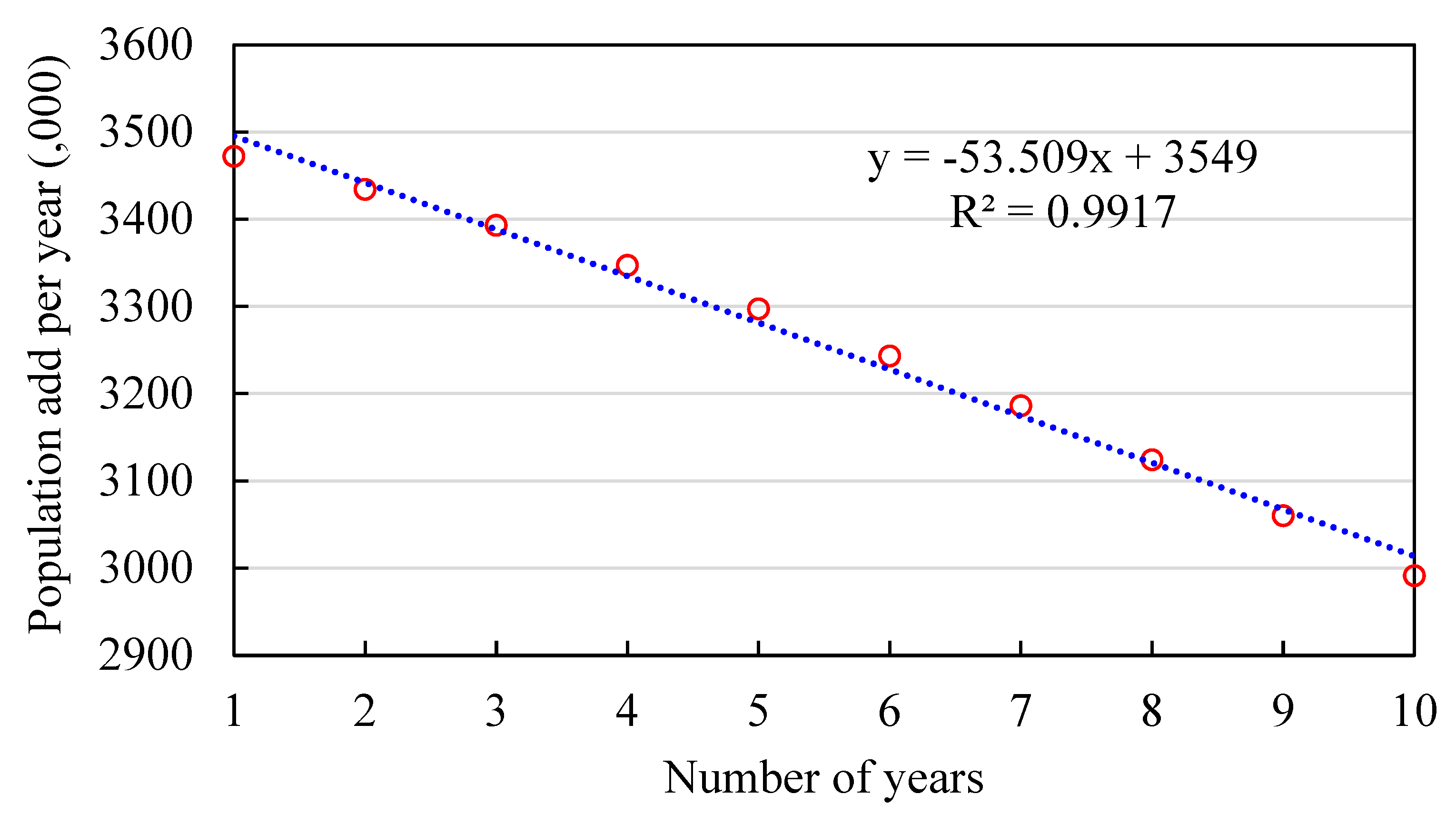
Table B2.
Projected population in Indonesia.
| X | Year | Growth (,000) | Population (,000) |
| 11 | 2021 | 2,960 | 274,026 |
| 12 | 2022 | 2,907 | 276,933 |
| 13 | 2023 | 2,853 | 279,787 |
| 14 | 2024 | 2,800 | 282,587 |
| 15 | 2025 | 2,746 | 285,333 |
| 16 | 2026 | 2,693 | 288,026 |
| 17 | 2027 | 2,639 | 290,665 |
| 18 | 2028 | 2,586 | 293,251 |
| 19 | 2029 | 2,532 | 295,783 |
| 20 | 2030 | 2,479 | 298,262 |
| 21 | 2031 | 2,425 | 300,687 |
| 22 | 2032 | 2,372 | 303,059 |
| 23 | 2033 | 2,318 | 305,378 |
| 24 | 2034 | 2,265 | 307,642 |
| 25 | 2035 | 2,211 | 309,854 |
| 26 | 2036 | 2,158 | 312,011 |
| 27 | 2037 | 2,104 | 314,116 |
| 28 | 2038 | 2,051 | 316,166 |
| 29 | 2039 | 1,997 | 318,164 |
| 30 | 2040 | 1,944 | 320,107 |
| 31 | 2041 | 1,890 | 321,998 |
| 32 | 2042 | 1,837 | 323,834 |
| 33 | 2043 | 1,783 | 325,617 |
| 34 | 2044 | 1,730 | 327,347 |
| 35 | 2045 | 1,676 | 329,023 |
| 36 | 2046 | 1,623 | 330,646 |
| 37 | 2047 | 1,569 | 332,215 |
| 38 | 2048 | 1,516 | 333,731 |
| 39 | 2049 | 1,462 | 335,193 |
| 40 | 2050 | 1,409 | 336,602 |
Appendix C
Supplementary methods
Table C1.
Basic data for the urban population in Indonesia.
| No | Year | Urban population (%) | Add. Per year (%) | Growth (%) |
| 2010 | 49.9 | |||
| 1 | 2011 | 50.6 | 0.69 | 1.38% |
| 2 | 2012 | 51.3 | 0.68 | 1.34% |
| 3 | 2013 | 52.0 | 0.68 | 1.33% |
| 4 | 2014 | 52.6 | 0.68 | 1.31% |
| 5 | 2015 | 53.3 | 0.67 | 1.27% |
| 6 | 2016 | 54.0 | 0.68 | 1.28% |
| 7 | 2017 | 54.7 | 0.67 | 1.24% |
| 8 | 2018 | 55.3 | 0.67 | 1.23% |
| 9 | 2019 | 56.0 | 0.66 | 1.19% |
| 10 | 2020 | 56.64 | 0.65 | 1.16% |
Supplementary results
Figure C1.
Trend of urban population growth in Indonesia.
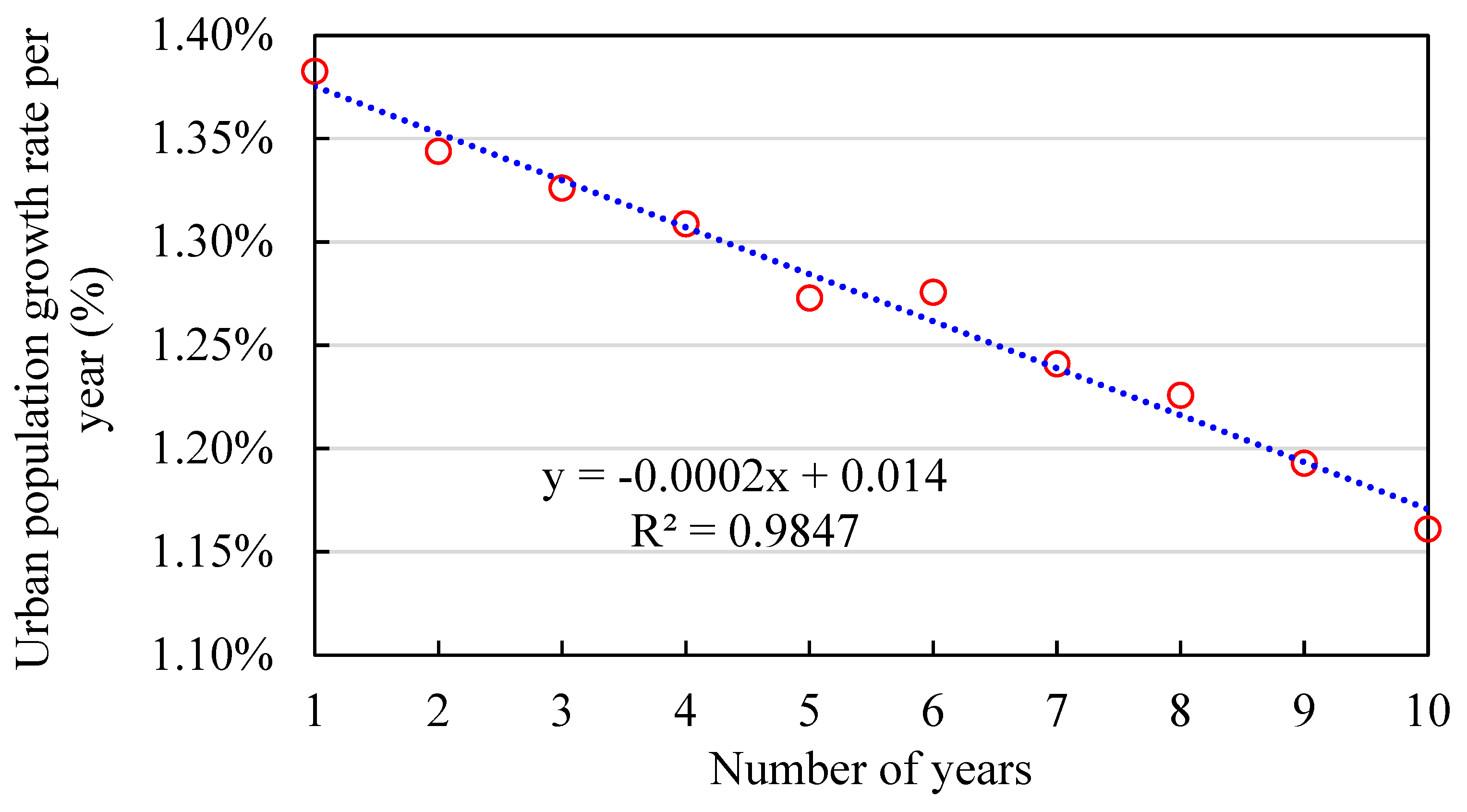
Table C2.
Projected urban population in Indonesia.
| X | Year | Growth rate (%) | Total urban population (%) |
| 2020 | 56.64% | ||
| 11 | 2021 | 1.18% | 57.82% |
| 12 | 2022 | 1.16% | 58.98% |
| 13 | 2023 | 1.14% | 60.12% |
| 14 | 2024 | 1.12% | 61.24% |
| 15 | 2025 | 1.10% | 62.34% |
| 16 | 2026 | 1.08% | 63.42% |
| 17 | 2027 | 1.06% | 64.48% |
| 18 | 2028 | 1.04% | 65.52% |
| 19 | 2029 | 1.02% | 66.54% |
| 20 | 2030 | 1.00% | 67.54% |
| 21 | 2031 | 0.98% | 68.52% |
| 22 | 2032 | 0.96% | 69.48% |
| 23 | 2033 | 0.94% | 70.42% |
| 24 | 2034 | 0.92% | 71.34% |
| 25 | 2035 | 0.90% | 72.24% |
| 26 | 2036 | 0.88% | 73.12% |
| 27 | 2037 | 0.86% | 73.98% |
| 28 | 2038 | 0.84% | 74.82% |
| 29 | 2039 | 0.82% | 75.64% |
| 30 | 2040 | 0.80% | 76.44% |
| 31 | 2041 | 0.78% | 77.22% |
| 32 | 2042 | 0.76% | 77.98% |
| 33 | 2043 | 0.74% | 78.72% |
| 34 | 2044 | 0.72% | 79.44% |
| 35 | 2045 | 0.70% | 80.14% |
| 36 | 2046 | 0.68% | 80.82% |
| 37 | 2047 | 0.66% | 81.48% |
| 38 | 2048 | 0.64% | 82.12% |
| 39 | 2049 | 0.62% | 82.74% |
| 40 | 2050 | 0.60% | 83.34% |
Appendix D
Supplementary methods
Table D1.
Basic data of labour productivity in Indonesia.
| No | Year | GDP per capita (000 IDR) | labour (000) | labour productivity (000 IDR) | Add. Per year (,000) | Growth (%) |
| 2009 | 5.606E+12 | 113833 | 49,248 | |||
| 2010 | 6.864E+12 | 116528 | 58,904 | 9,657 | 19.61% | |
| 1 | 2011 | 7.832E+12 | 117370 | 66,729 | 7,825 | 13.28% |
| 2 | 2012 | 8.616E+12 | 118053 | 72,984 | 6,255 | 9.37% |
| 3 | 2013 | 9.546E+12 | 118193 | 80,766 | 7,782 | 10.66% |
| 4 | 2014 | 1.057E+13 | 121873 | 86,730 | 5,963 | 7.38% |
| 5 | 2015 | 1.1526E+13 | 114819 | 100,384 | 13,654 | 15.74% |
| 6 | 2016 | 1.2407E+13 | 118412 | 104,778 | 4,394 | 4.38% |
| 7 | 2017 | 1.359E+13 | 121022 | 112,294 | 7,515 | 7.17% |
| 8 | 2018 | 1.4839E+13 | 126282 | 117,507 | 5,213 | 4.64% |
| 9 | 2019 | 1.5834E+13 | 128755 | 122,978 | 5,471 | 4.66% |
Table D2.
Basic data of labour participation rate in Indonesia.
| labour (000) | Population (,000) | labour participation rate |
| 113833 | 234757 | 0.484897 |
| 116528 | 238519 | 0.488548 |
| 117370 | 241991 | 0.485018 |
| 118053 | 245425 | 0.481015 |
| 118193 | 248818 | 0.475018 |
| 121873 | 252165 | 0.483307 |
| 114819 | 255462 | 0.449456 |
| 118412 | 258705 | 0.457711 |
| 121022 | 261891 | 0.462108 |
| 126282 | 265015 | 0.476509 |
| 128755 | 268075 | 0.480295 |
| 128066 | 271066 | 0.472453 |
Supplementary results
Table D3.
Projected labour productivity.
| Year | Labour productivity (%) |
| 2020 | 5.09252 |
| 2021 | 4.84105 |
| 2022 | 4.6207 |
| 2023 | 4.42565 |
| 2024 | 4.25146 |
| 2025 | 4.09473 |
| 2026 | 3.95277 |
| 2027 | 3.82344 |
| 2028 | 3.705 |
| 2029 | 3.59603 |
| 2030 | 3.49536 |
| 2031 | 3.40199 |
| 2032 | 3.31511 |
| 2033 | 3.234 |
| 2034 | 3.15807 |
| 2035 | 3.0868 |
| 2036 | 3.01974 |
| 2037 | 2.95649 |
| 2038 | 2.89673 |
| 2039 | 2.84013 |
| 2040 | 2.78645 |
| 2041 | 2.73543 |
| 2042 | 2.68688 |
| 2043 | 2.6406 |
| 2044 | 2.59642 |
| 2045 | 2.5542 |
| 2046 | 2.51379 |
| 2047 | 2.47508 |
| 2048 | 2.43794 |
| 2049 | 2.40228 |
| 2050 | 2.36801 |
Figure D1.
Trend of labour productivity in Indonesia.
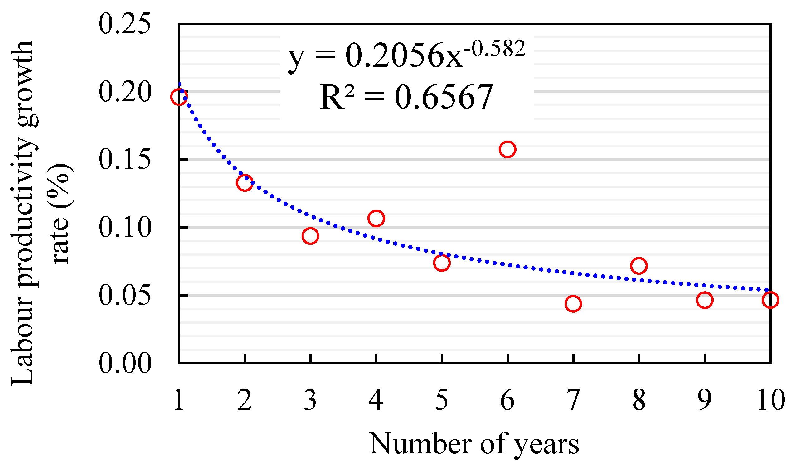
Figure D2.
Trend of the labour participation rate in Indonesia.
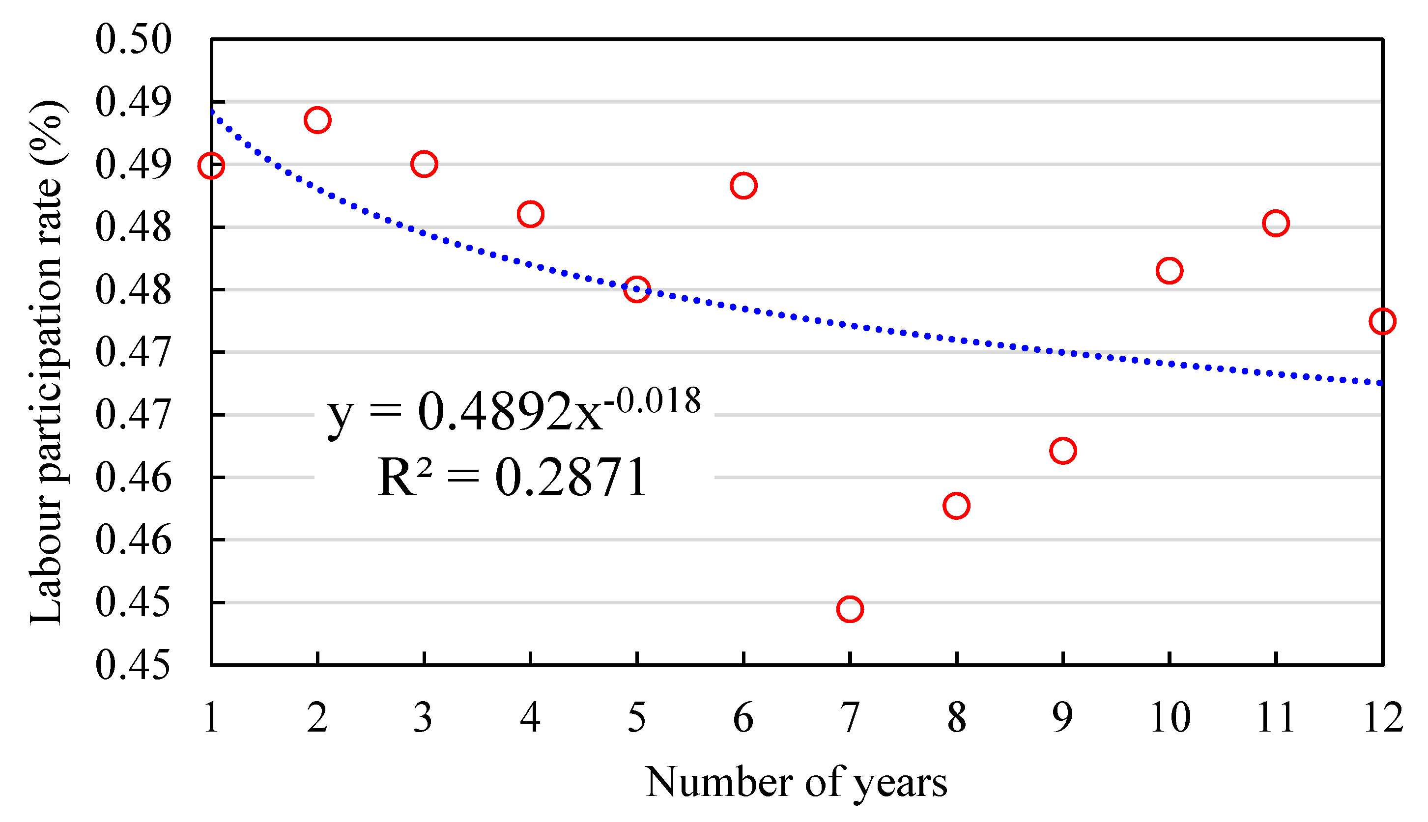
Table D4.
Projected labour participation rate.
| Year | Labour participation rate (%) |
| 2020 | 47.2453 |
| 2021 | 46.7128 |
| 2022 | 46.6505 |
| 2023 | 46.5926 |
| 2024 | 46.5385 |
| 2025 | 46.4877 |
| 2026 | 46.4399 |
| 2027 | 46.3948 |
| 2028 | 46.3519 |
| 2029 | 46.3112 |
| 2030 | 46.2725 |
| 2031 | 46.2355 |
| 2032 | 46.2001 |
| 2033 | 46.1661 |
| 2034 | 46.1336 |
| 2035 | 46.1022 |
| 2036 | 46.0721 |
| 2037 | 46.043 |
| 2038 | 46.0149 |
| 2039 | 45.9877 |
| 2040 | 45.9615 |
| 2041 | 45.936 |
| 2042 | 45.9113 |
| 2043 | 45.8874 |
| 2044 | 45.8641 |
| 2045 | 45.8415 |
| 2046 | 45.8195 |
| 2047 | 45.7981 |
| 2048 | 45.7772 |
| 2049 | 45.7569 |
| 2050 | 45.737 |
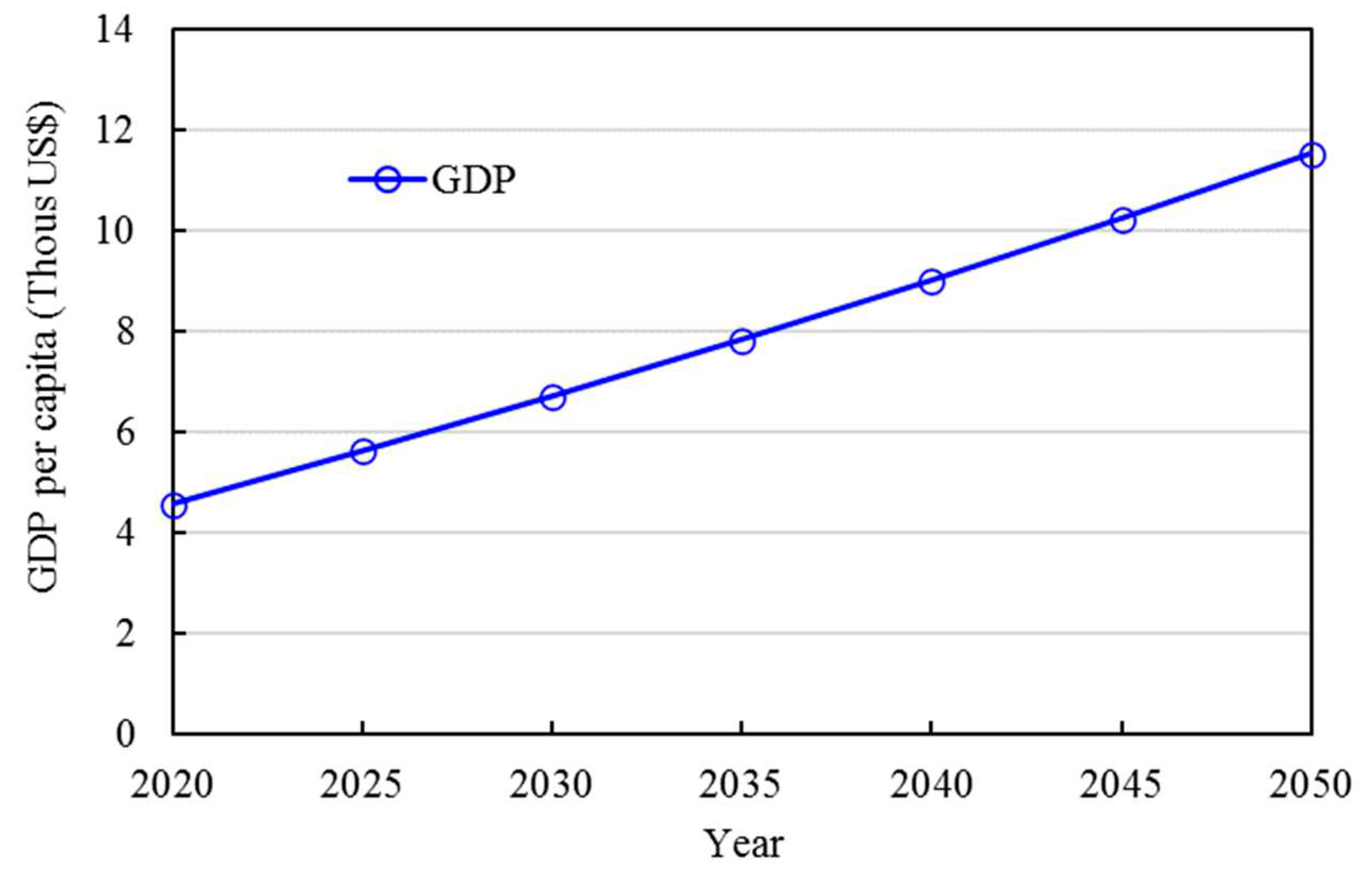
Figure D3.
GDP for the urban population in Indonesia.
Appendix E
Appendix F
References
- Ianchenko, A. Simonen, and C. Barnes, Residential building lifespan and community turnover. Journal of Architectural Engineering, 2020. 26(3): p. 04020026. [CrossRef]
- O'Neil, A. indonesia: Urbanisation from 2110 to 2020. 2021 [cited 2021 29th September].
- Worldometer. Indonesia population. 2021 [cited 2021 19th August ]; Available from: https://www.worldometers.info/world-population/indonesia-population/.
- Tumiwa, F. Climate transparency report - comparing G20 climate action and responses to the COVID-19 crisis. 2020 [cited 2021 24 November]; Available from: https://www.climate-transparency.org/wp-content/uploads/2020/11/Indonesia-CT-2020-WEB.pdf.
- Adi, A.C. , et al., Handbook of energy and economic statistics of Indonesia. 2021.
- McBain, B. , et al., Building Robust Housing Sector Policy Using the Ecological Footprint. Resources, 2018. 7(2): p. 24. [CrossRef]
- GBPN. Healthy buildings, healthy lives. 2021 [cited 2021 20 December]; Available from: https://www.gbpn.org/healthy-buildings-healthy-lives/.
- UNFCC. First Nationally Determined Contribution-Republic of Indonesia. 2021 [cited 2021 1 December]; Available from: https://www4.unfccc.int/sites/NDCStaging/Pages/Party.aspx?party=IDN.
- Clarke, L. , et al., Effects of long-term climate change on global building energy expenditures. Energy Economics, 2018. 72: p. 667-677. [CrossRef]
- Fricko, O. , et al., The marker quantification of the Shared Socioeconomic Pathway 2: A middle-of-the-road scenario for the 21st century. Global Environmental Change, 2017. 42: p. 251-267. [CrossRef]
- Building, J.G. Jakarta green building user guide Vol. 1 building envelope. 2021 [cited 2021 14th September]; Available from: https://greenbuilding.jakarta.go.id/files/userguides/Vol-1-BuildingEnvelope-UserGuide.pdf.
- Hajji, A.M. and A.R.Z. Hilmi, Façade design modification in complying the Indonesia’s national standard of energy conservation for tall building envelope – Case study: Green Office Park 9, Serpong, Indonesia. IOP Conference Series: Earth and Environmental Science, 2021. 847(1): p. 012028. [CrossRef]
- Silalahi, D.F. , et al., Indonesia’s Vast Solar Energy Potential. Energies, 2021. 14(17): p. 5424. [CrossRef]
- Hapsari Damayanti, F. Tumiwa, and M. Citraningrum, Residential Rooftop Solar Technical and Market Potential in 34 Provinces in Indonesia. 2019: IESR: Jakarta, Indonesia. p. Pages 1-17.
- Donker, J. and X. van Tilburg, Three Indonesian solar-powered futures. Solar PV and ambitious climate policy. 2019.
- Nasional, D.E. , Technology Data for the Indonesian Power Sector: Catalogue for Generation and Storage of Electricity. 2021, Dewan Energi Nasional. Dewan Energi Nasional, Jakarta, Indonesia.
- Singh, R. and R. Banerjee, Estimation of rooftop solar photovoltaic potential of a city. Solar Energy, 2015. 115: p. 589-602. [CrossRef]
- Widaningsih, L., T. Megayanti, and R. Minggra, Floor-Area Ratio in the Eastern Corridor of Jalan Ir. H. Djuanda Bandung. 2016.
- Rating, E. HEAT PUMP WATER HEATERS. 2021 [cited 2021 19th November]; Available from: https://www.energyrating.gov.au/products/water-heaters/heat-pump-water-heaters.
- Taqwim, S., N. Saptadji, and A. Ashat, MEASURING THE POTENTIAL BENEFITS OF GEOTHERMAL COOLING AND HEATING APPLICATIONS IN INDONESIA. 2013.
- Yasukawa, K. and Y. Uchida, Space Cooling by Ground Source Heat Pump in Tropical Asia, in Renewable Geothermal Energy Explorations. 2018, IntechOpen.
- Miyara, A. , et al. Development of an open-loop ground source cooling system for space air conditioning system in hot climate like Indonesia. in MATEC Web of Conferences. 2018. EDP Sciences.
- Wilson, P. Building regulations and land use in the spatial plan. 2015 [cited 2021 2nd October]; Available from: https://www.mrfixitbali.com/building-construction/licences-permits-and-zoning/building-regulations-denpasar-sanur-227.html.
- Sahid, Y. Sumiyati, and R. Purisari, The Direction of Developing Green Building Criteria in Indonesia. Journal of Physics: Conference Series, 2021. 1811(1): p. 012090. [CrossRef]
- Sahid, Y. Sumiyati, and R. Purisari, The Constrains of Green Building Implementation in Indonesia. Journal of Physics: Conference Series, 2020. 1485: p. 012050. [CrossRef]
- Berawi, M.A. , et al., Stakeholders' perspectives on green building rating: A case study in Indonesia. Heliyon, 2019. 5(3): p. e01328. [CrossRef]
- Tumiwa, F. The G20 transition to a low carbon economy. 2018 [cited 2021 24 November]; Available from: https://www.climate-transparency.org/wp-content/uploads/2019/01/BROWN-TO-GREEN_2018_Indonesia_FINAL.pdf.
- GBPN. Low carbon residential buildings regulatory reform. 2021 [cited 2021 20 December]; Available from: https://www.gbpn.org/projects/low-carbon-residential-buildings-regulatory-reform/. /: 2021 20 December]; Available from: https.
- GBPN. Review of incentives on green bilding regulatoins. 2021 [cited 2021 20 December]; Available from: https://www.gbpn.org/projects/review-of-incentives-on-green-building-regulations/. /.
- EN, B. , Sustainability of Construction Works Assessment of Environmental Performance of Buildings Calculation Method. BS EN, 2011. 15978: p. 2011.
- Kolokolov, A. labor productivity and other adventures. 2020 [cited 2021 30th September]; Available from: https://towardsdatascience.com/labor-productivity-and-other-adventures-67212d1d199b.
- Kyle, P., et al. Global Change Assessment Model (GCAM) Tutorial. 2017 [cited 2021 3 December]; Available from: http://www.globalchange.umd.edu/data/annual-meetings/2017/GCAM_Tutorial_2017.pdf. /.
- Dewi, J. Siahaan, and R.R. Tobing, Parametric simulation as a tool for observing relationships between parcel and regulations in unplanned commercial corridor. Procedia-Social and Behavioral Sciences, 2016. 227: p. 152-159.
- Herlambang, S. , et al., Jakarta’s great land transformation: Hybrid neoliberalisation and informality. Urban Studies, 2019. 56(4): p. 627-648.
- Energy. Heating and cooling. 2021 [cited 2021 15th September]; Available from: https://www.energy.gov.au/households/heating-and-cooling. /.
- Energysage. What are the most energy efficient appliances and are they worth it? 2021 [cited 2021 3rd October]; Available from: https://www.energysage.com/energy-efficiency/costs-benefits/energy-star-rebates/. /.
- Boretti, A. , et al. Capacity factors of solar photovoltaic energy facilities in California, annual mean and variability. in E3S Web of Conferences. 2020. EDP Sciences. 2020. [Google Scholar]
- Tracker, C.A. Country summary, Indonesia. 2021 [cited 2021 14 December]; Available from: https://climateactiontracker.org/countries/indonesia/.
Figure 1.
Total life cycle carbon stages in the building.
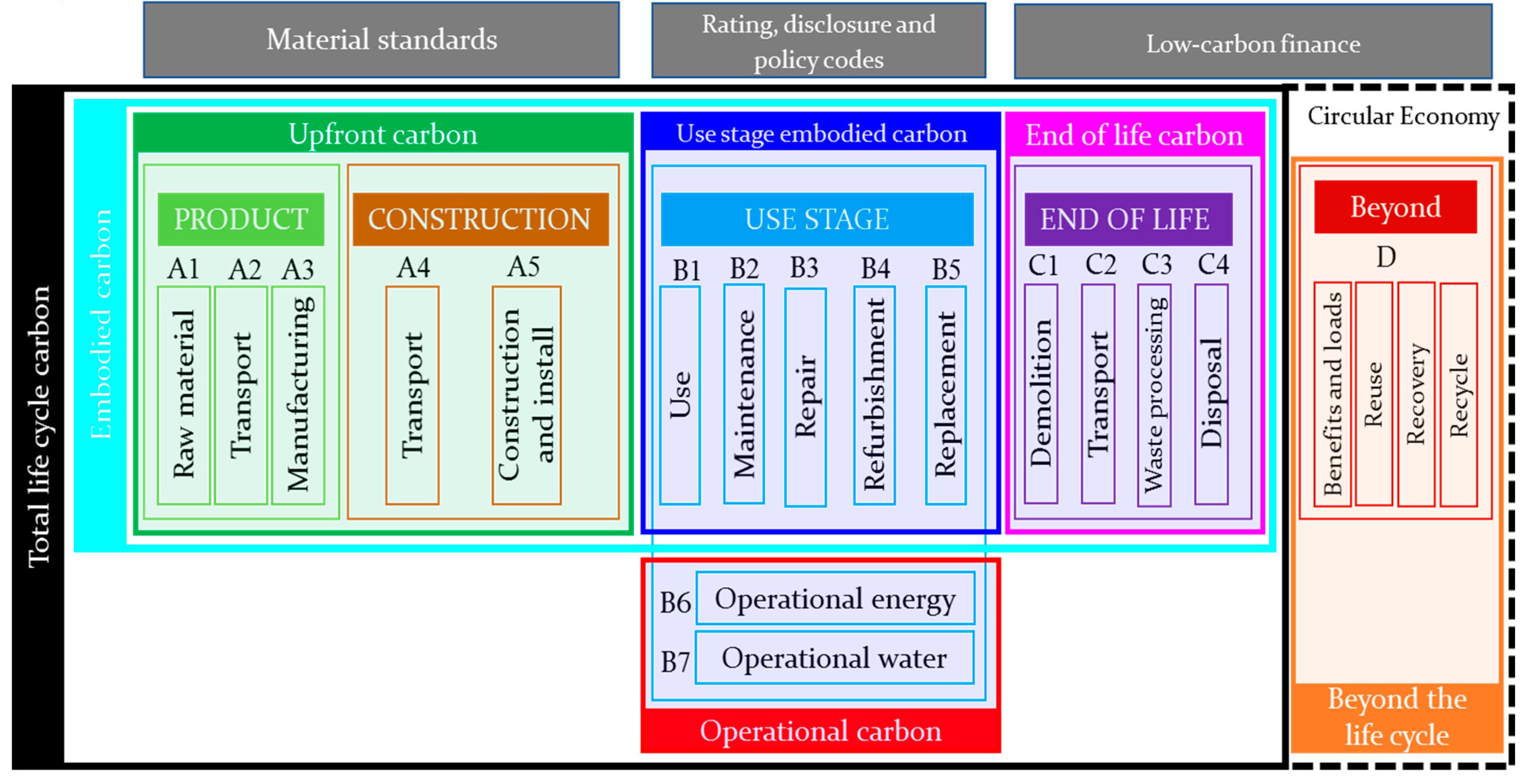
Figure 2.
Concept of net zero-carbon buildings.
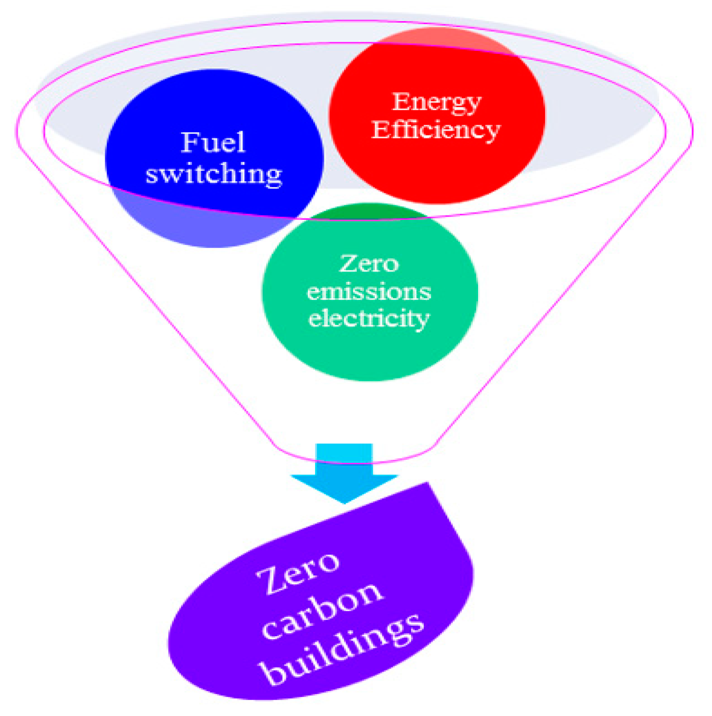
Figure 3.
(a) concept of rooftop PV in residential building, (b) concept of ground source heat pump system with residential building.
Figure 3.
(a) concept of rooftop PV in residential building, (b) concept of ground source heat pump system with residential building.
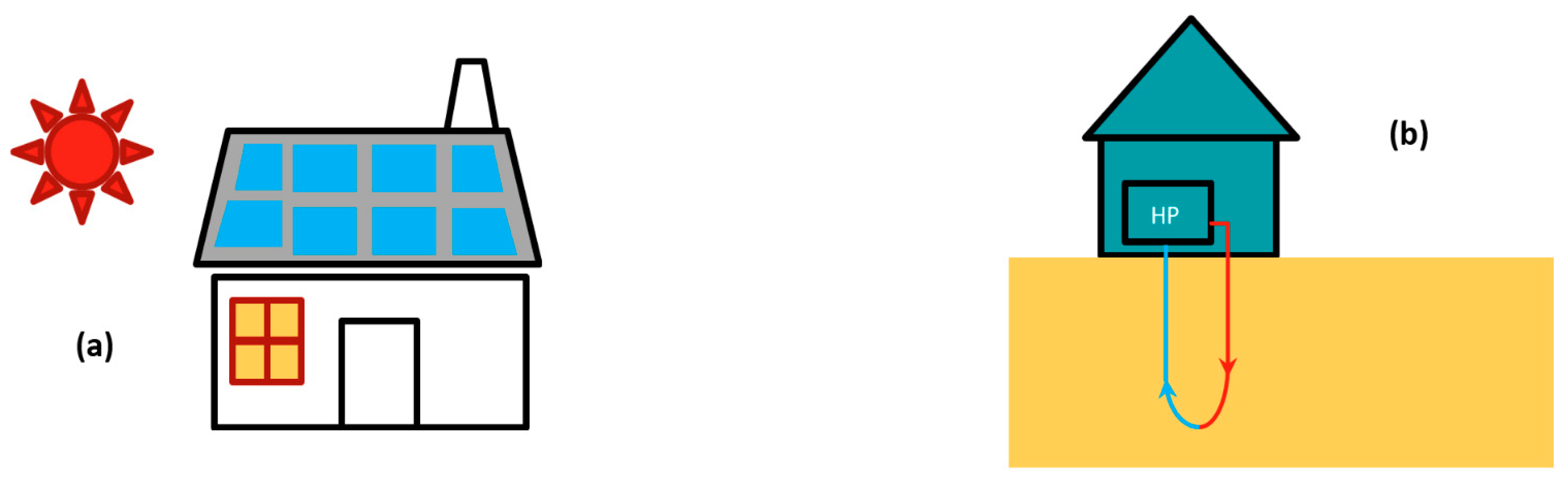
Figure 4.
Structure of energy demand and supply in Indonesian urban residential buildings.
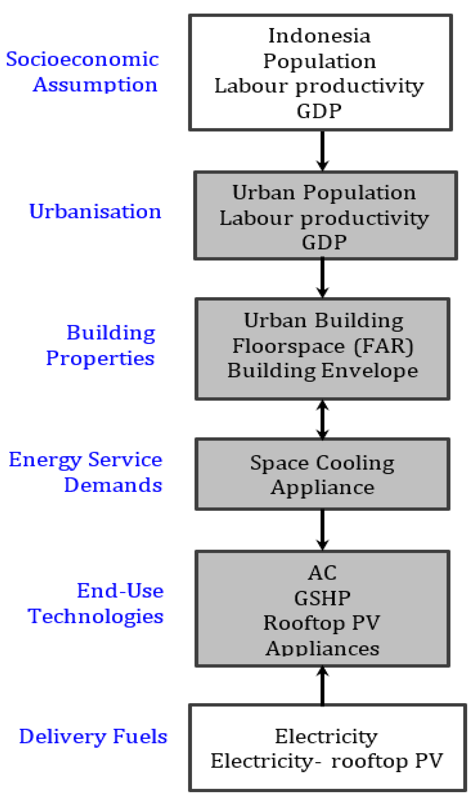
Figure 5.
Projected urban population in Indonesia.
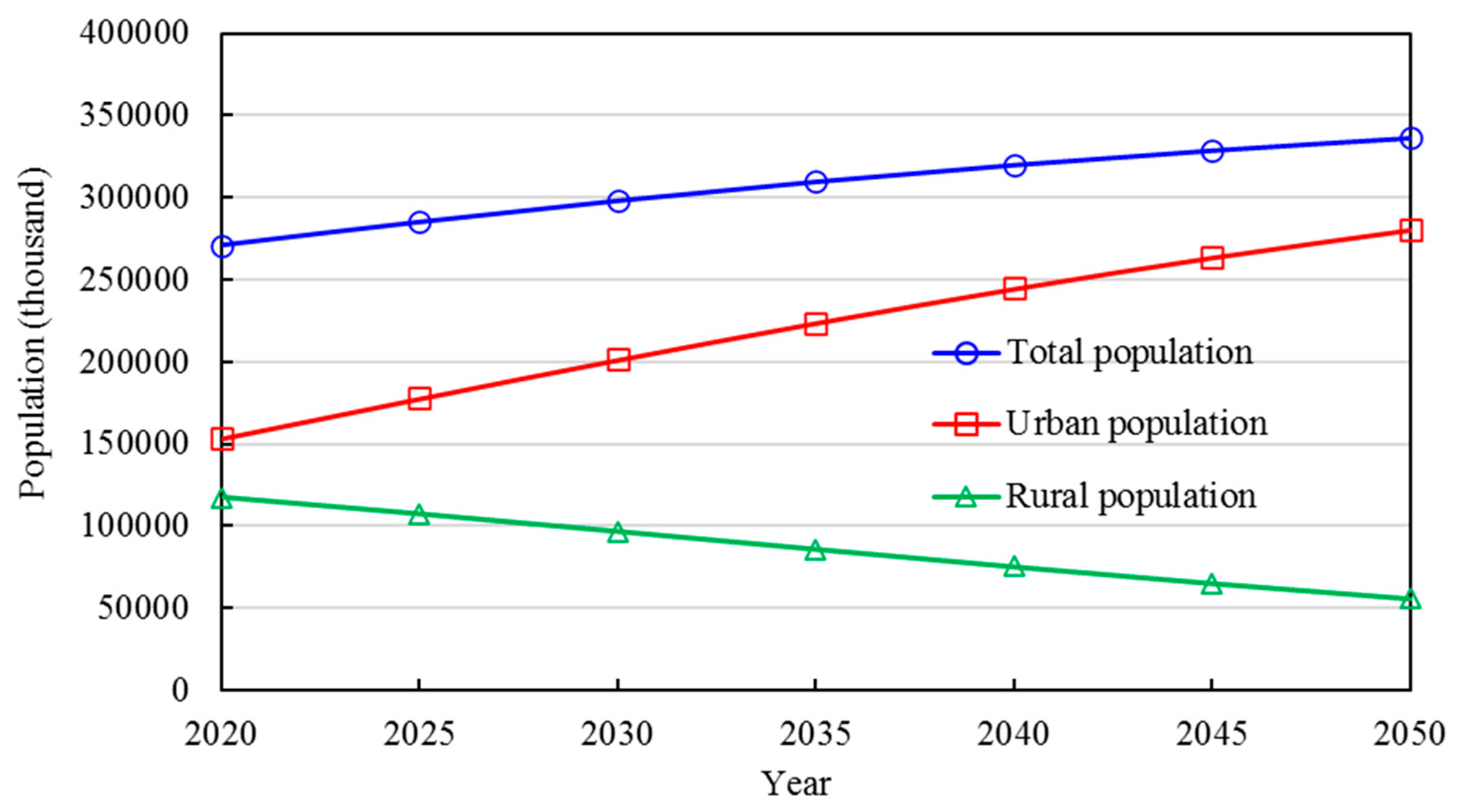
Figure 6.
Predicted labour productivity and labour participation rate in Indonesia.
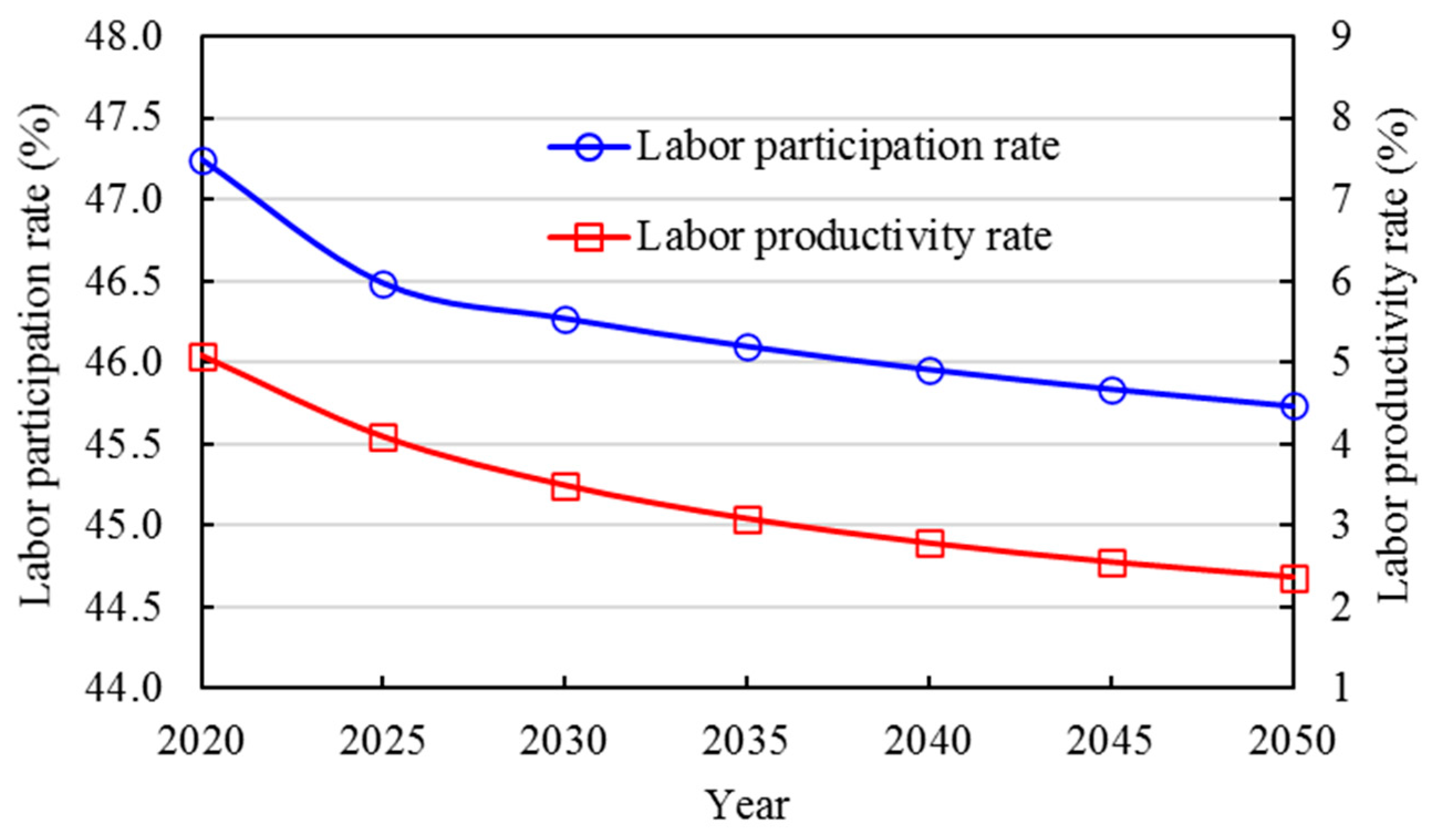
Figure 7.
Predicted future shell conductance (u-value) of building envelope.
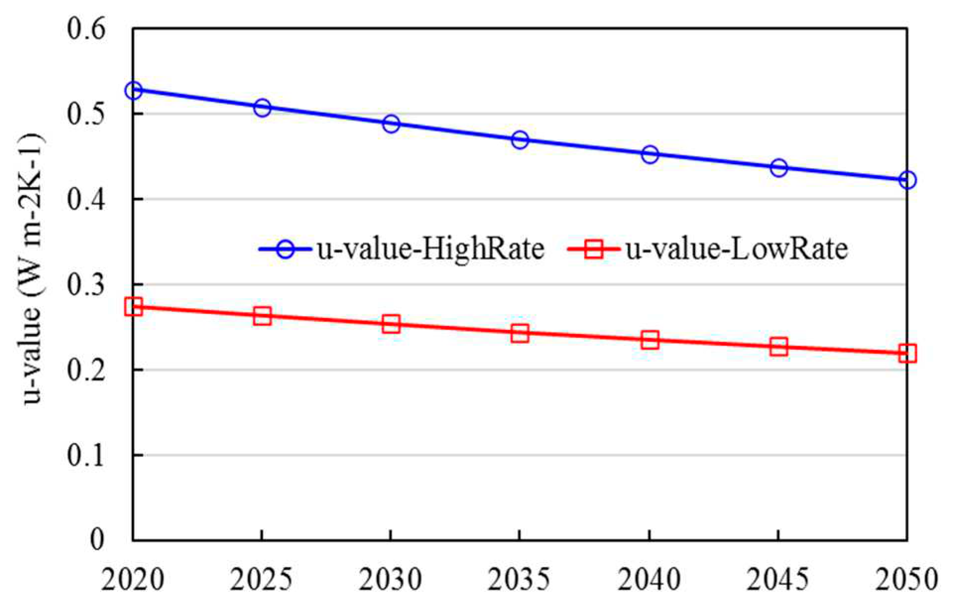
Figure 8.
Predicted AC efficiency input data for cooling application.
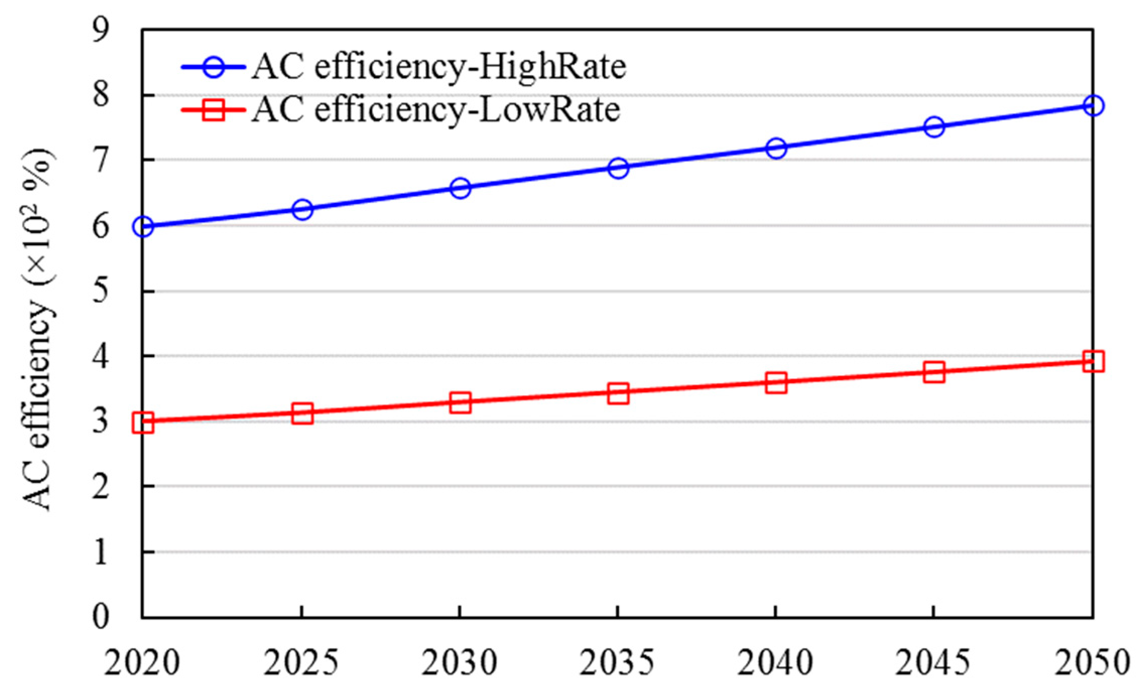
Figure 9.
Predicted future appliances (APLs) efficiency.
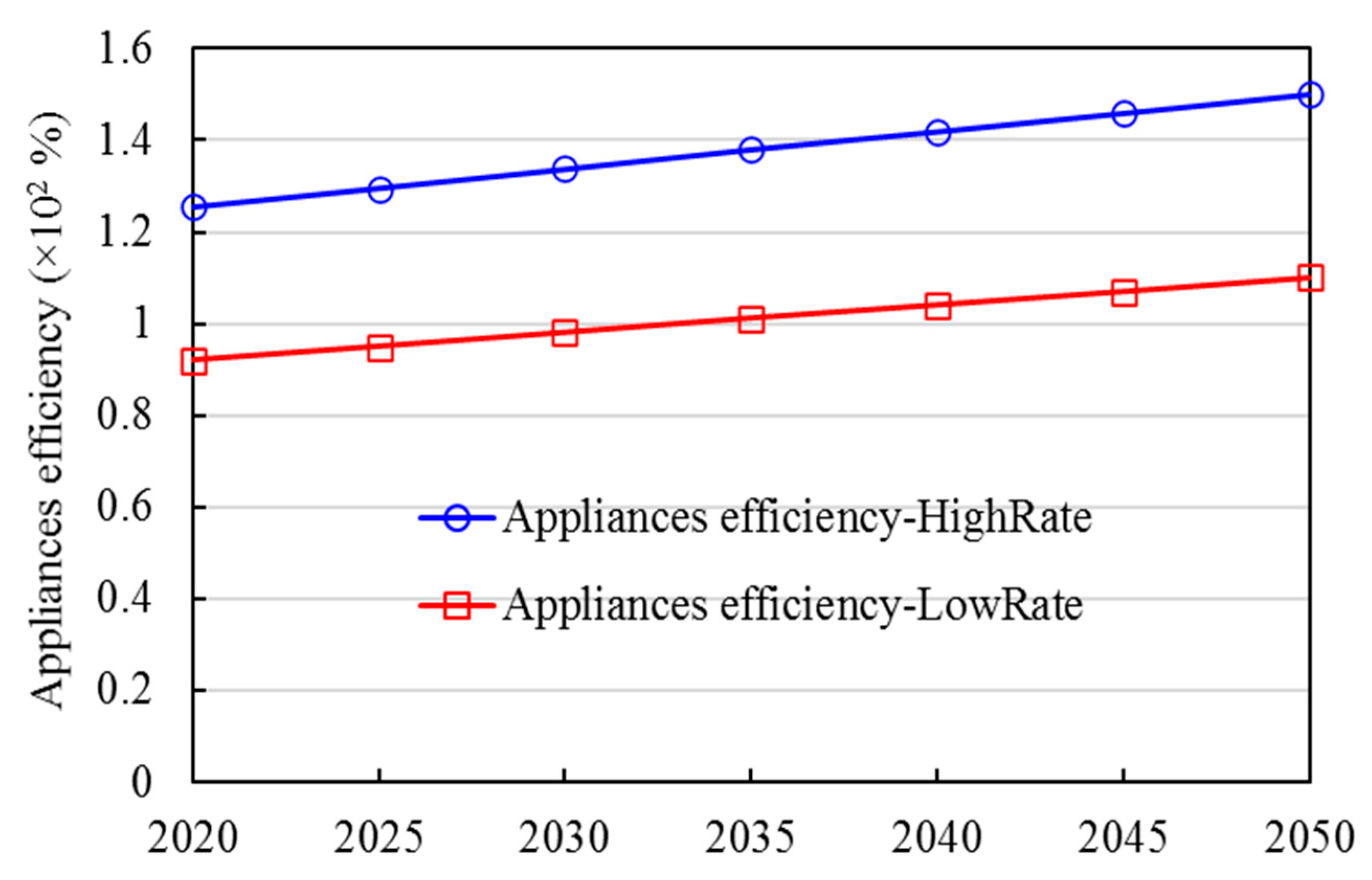
Figure 10.
Research framework and steps.
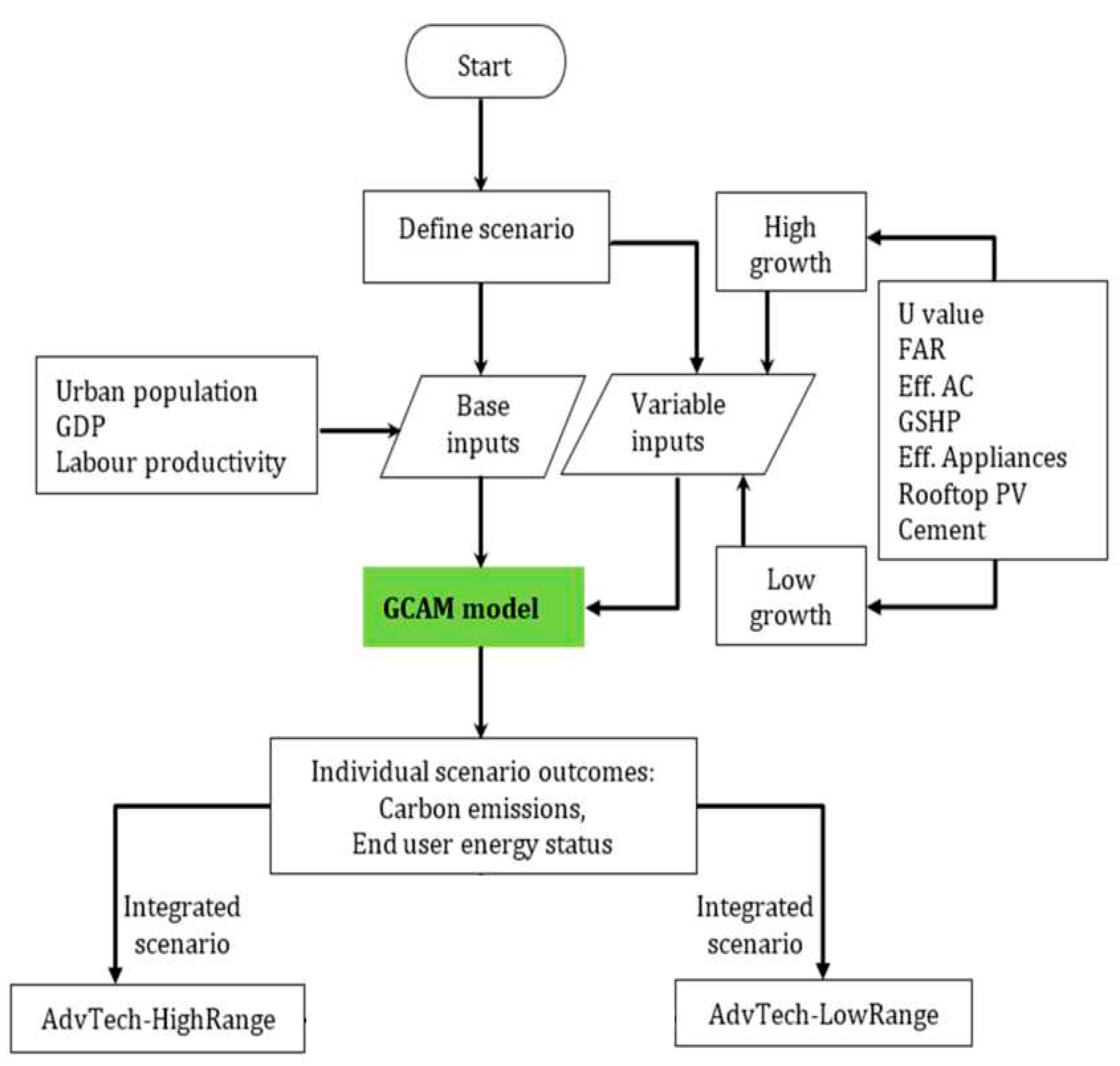
Figure 11.
Potential carbon emissions mitigation by U-value.
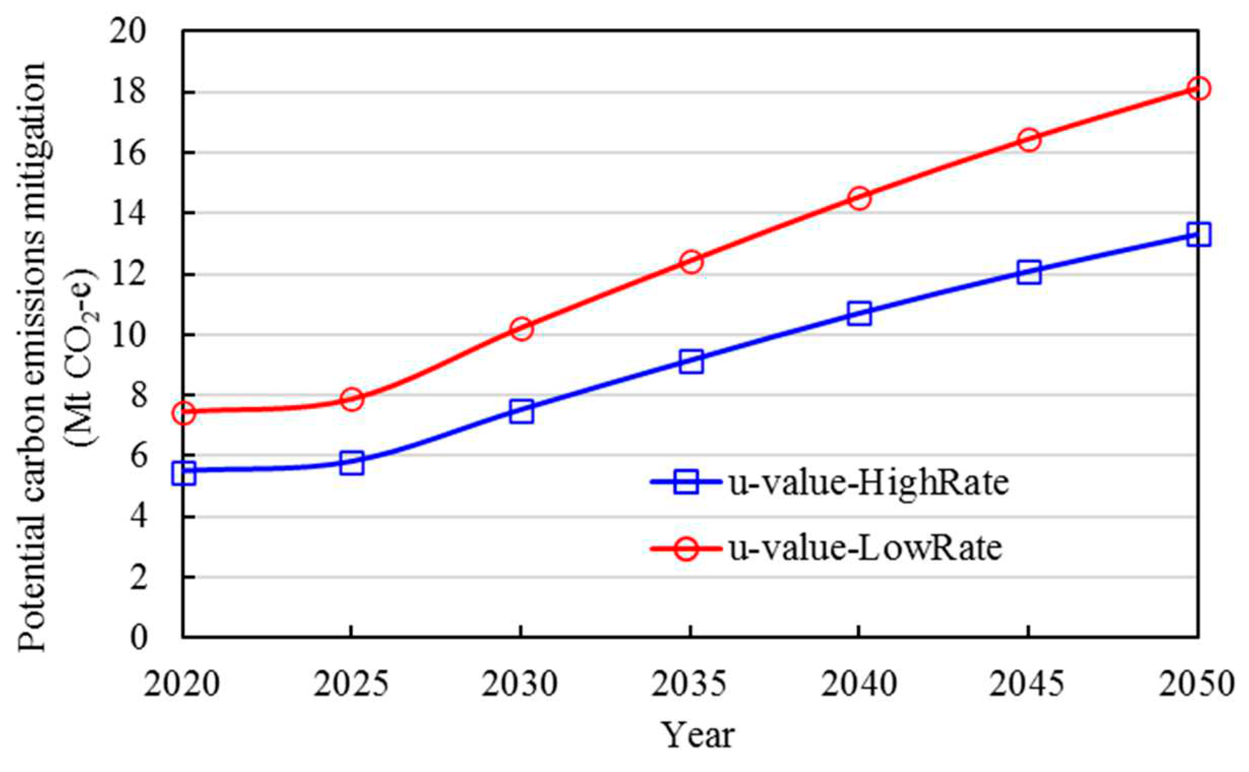
Figure 12.
Potential carbon emissions mitigation by FAR.
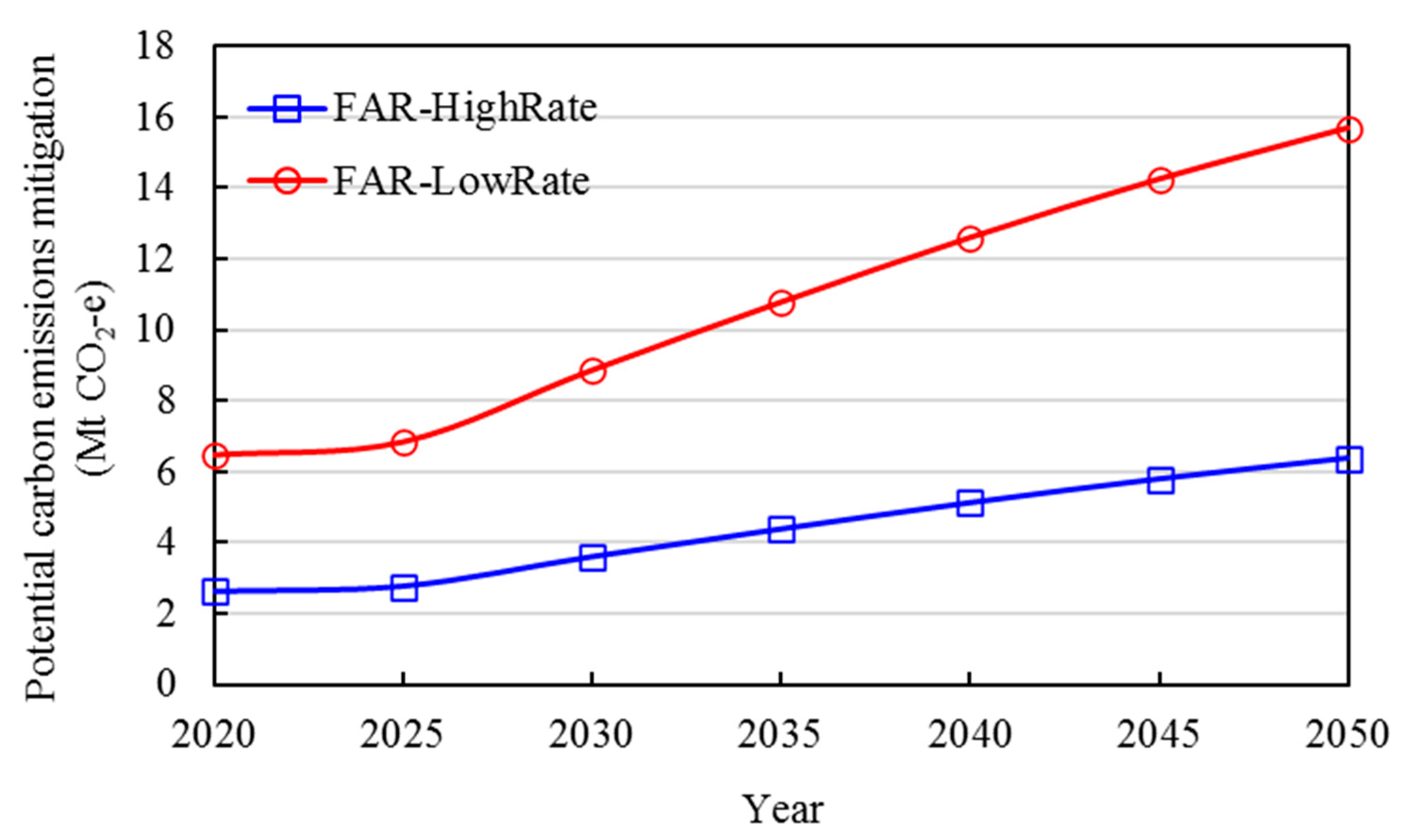
Figure 13.
Potential carbon emissions mitigation by AC efficiency.

Figure 14.
Potential carbon emissions mitigation by GSHP.
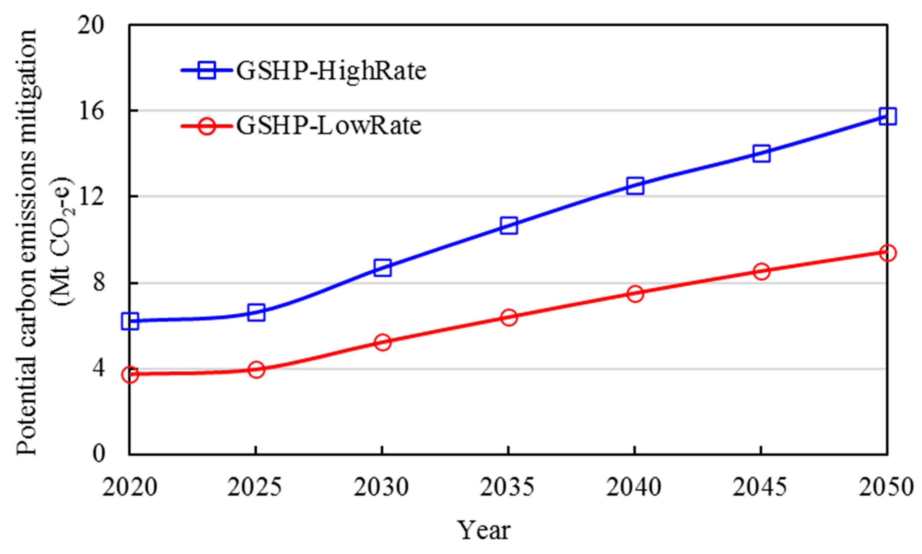
Figure 15.
Potential carbon emissions mitigation by appliance efficiency.
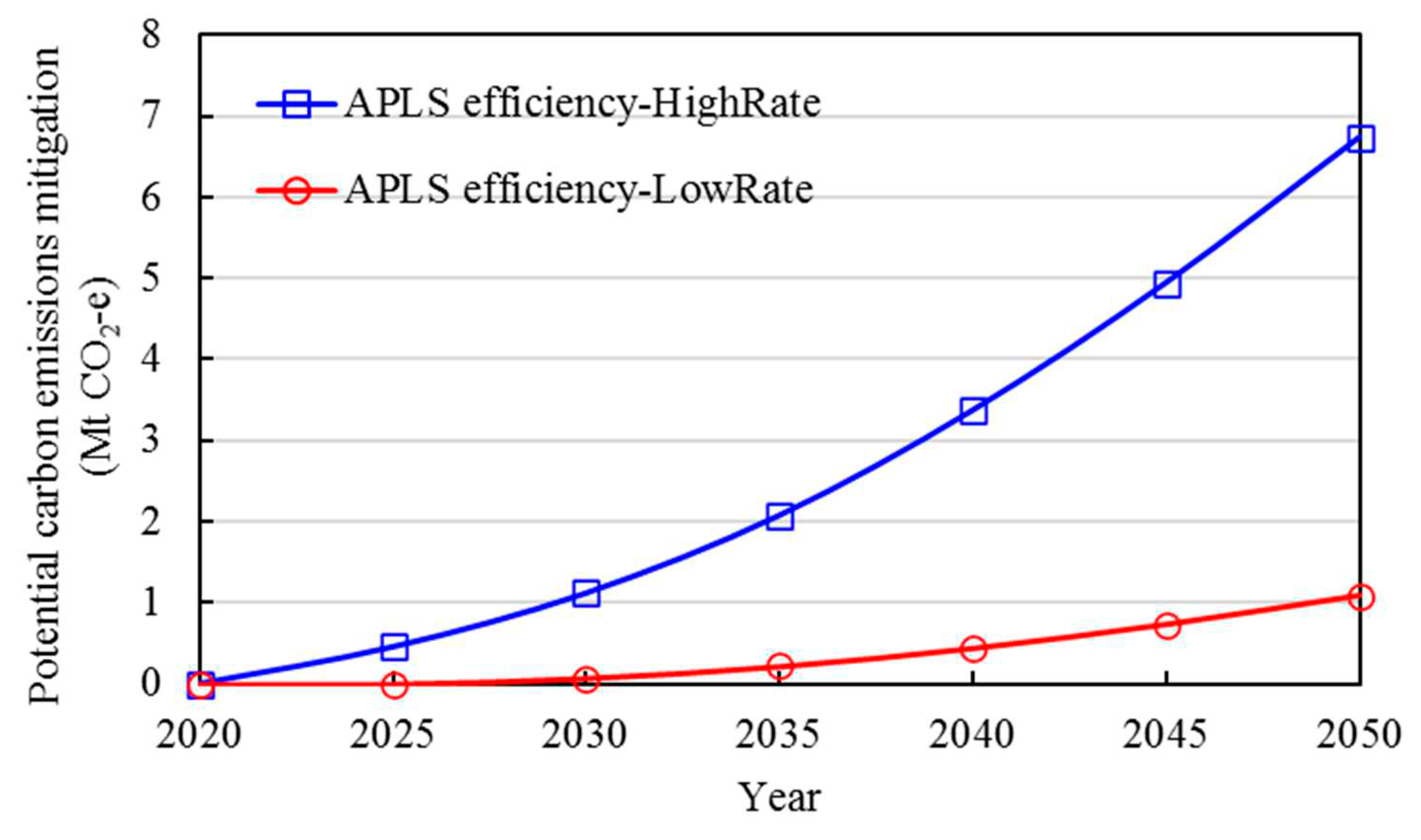
Figure 16.
Potential carbon emissions mitigation by rooftop PV (RTPV).
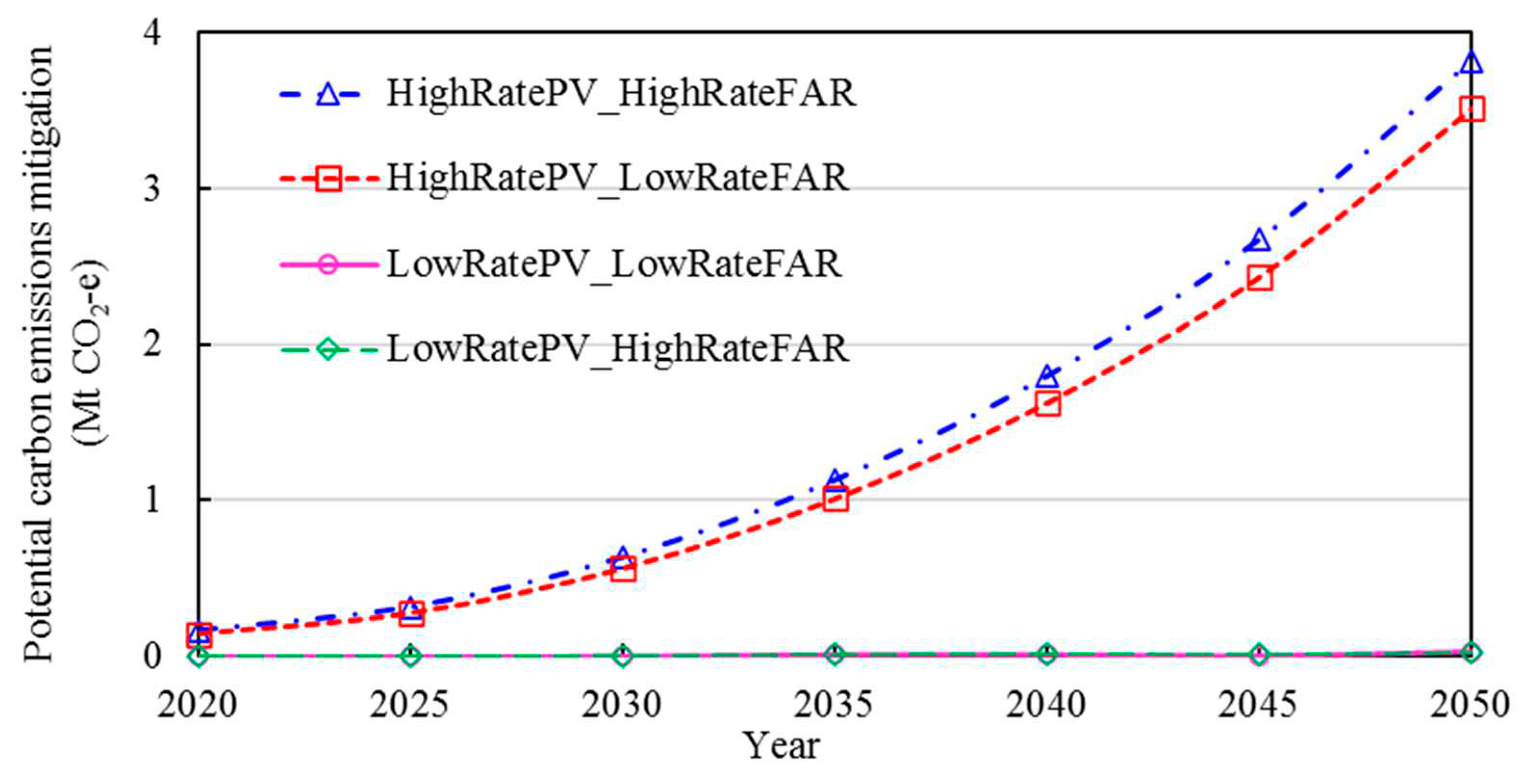
Figure 17.
Potential electricity production by rooftop PV.

Figure 18.
Effect of FAR on produced electricity by rooftop PV.
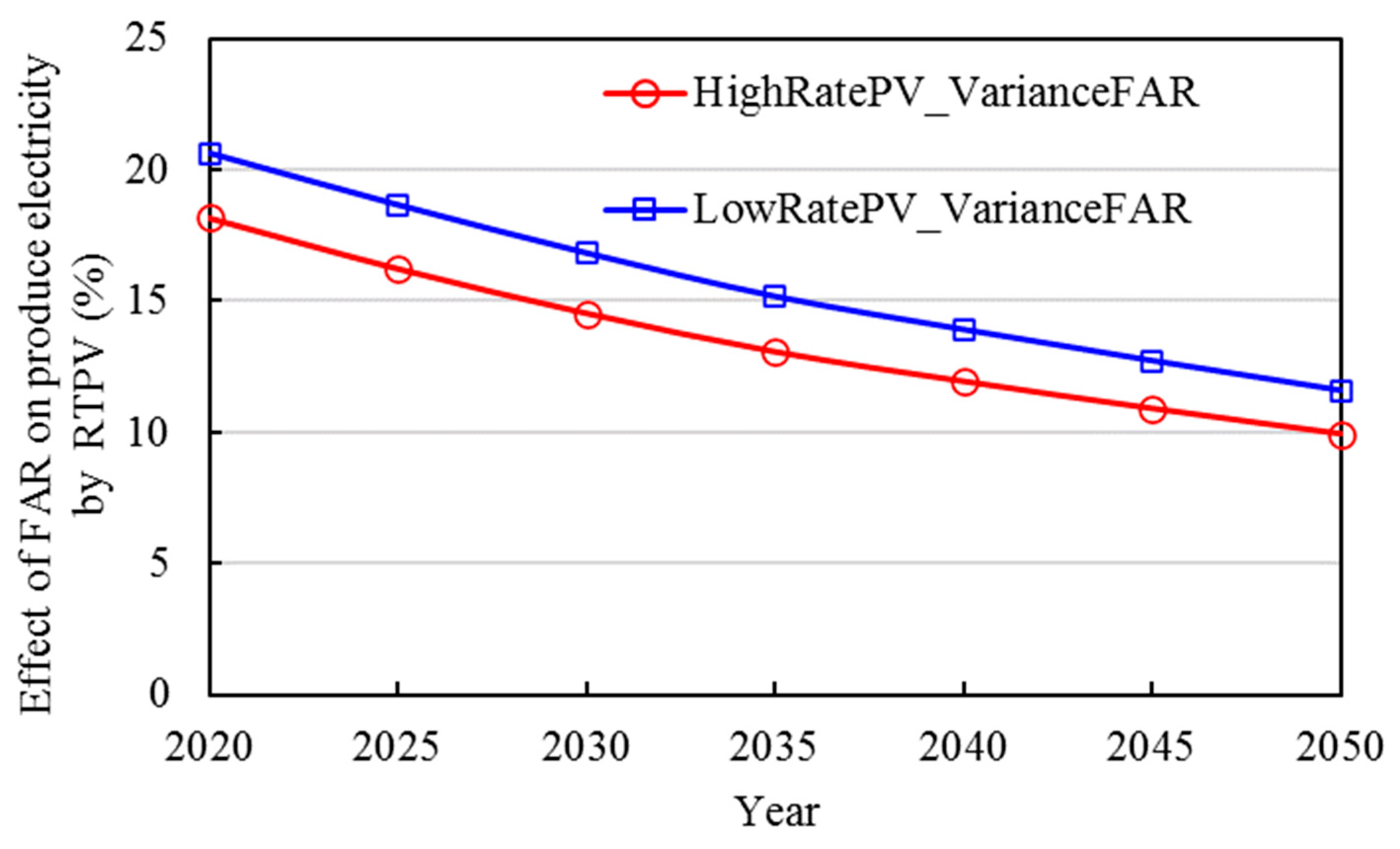
Figure 19.
Energy demand and supply status by rooftop PV, (a) LowRatePV_HighRateFAR, (b) LowRatePV_LowRateFAR, (c) HighRatePV_LowRateFAR, (d) HighRatePV_HighRateFAR.
Figure 19.
Energy demand and supply status by rooftop PV, (a) LowRatePV_HighRateFAR, (b) LowRatePV_LowRateFAR, (c) HighRatePV_LowRateFAR, (d) HighRatePV_HighRateFAR.
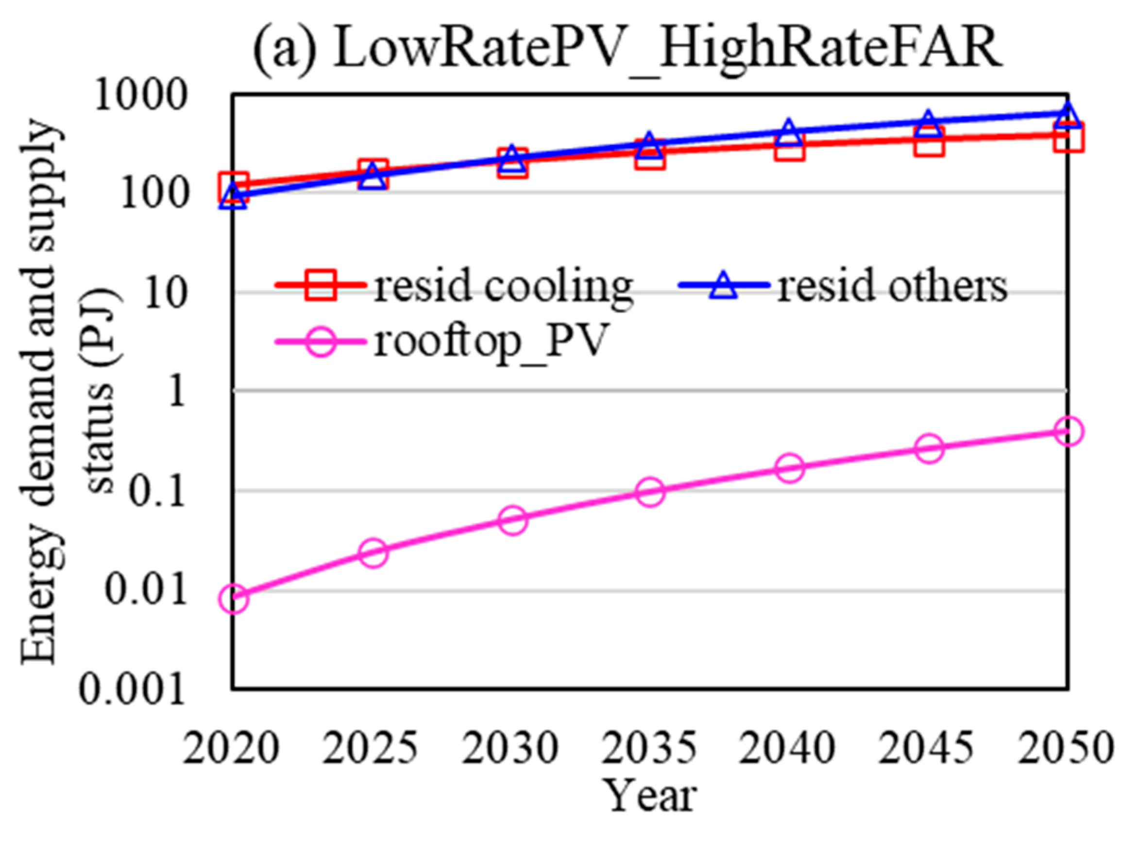
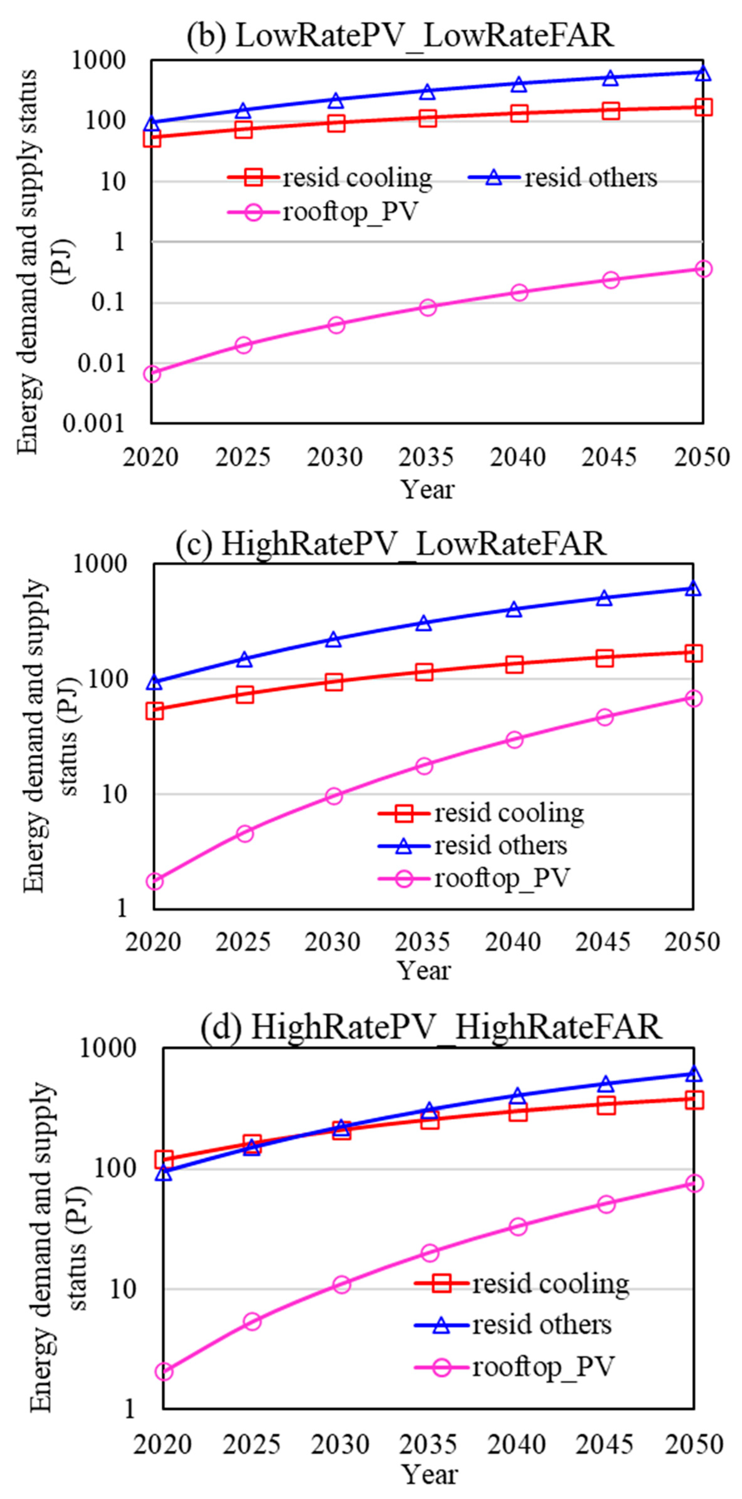
Figure 20.
Status of cooling demand reduction by rooftop PV.
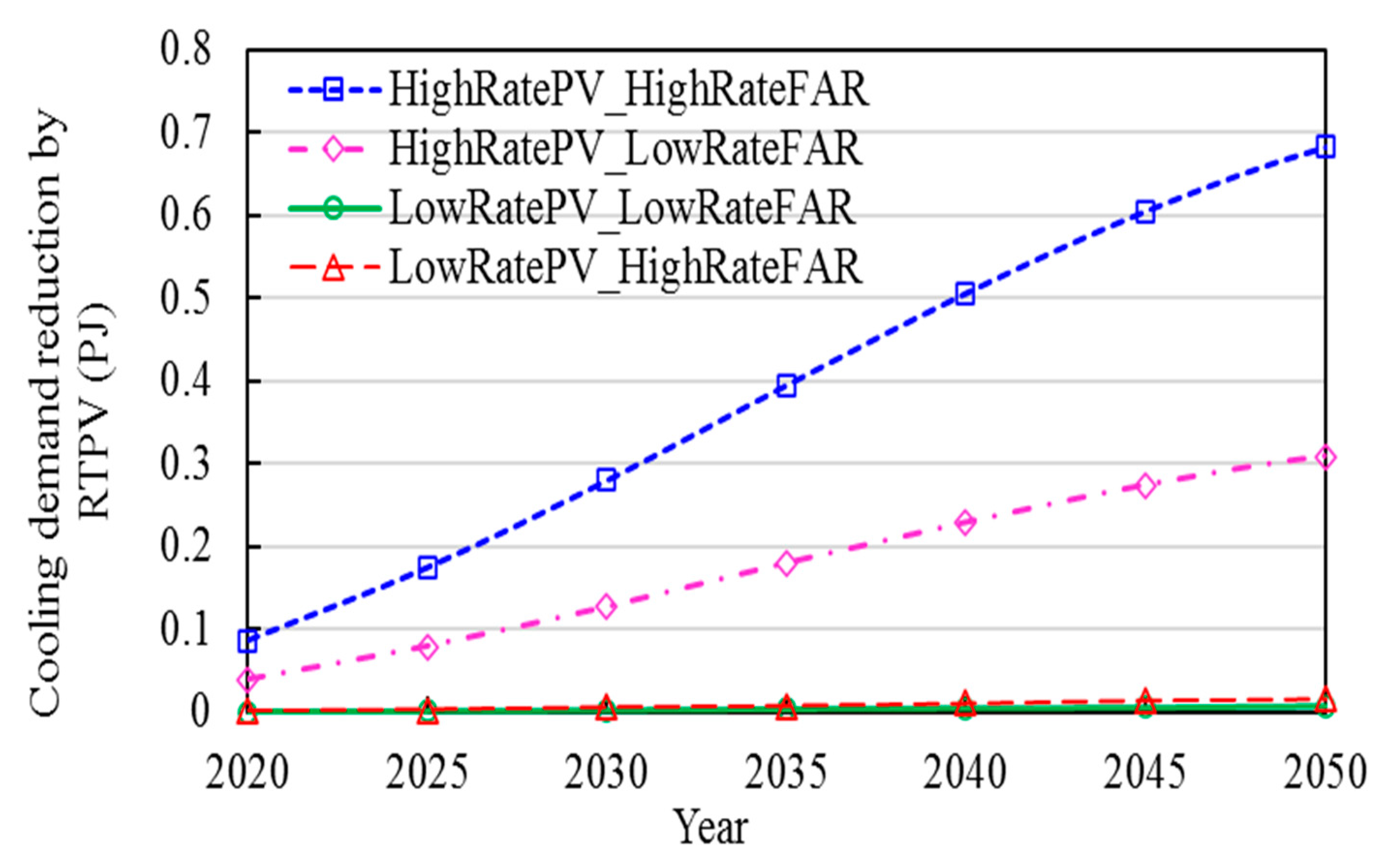
Figure 21.
Potential mitigation of indirect carbon emissions by cement production.
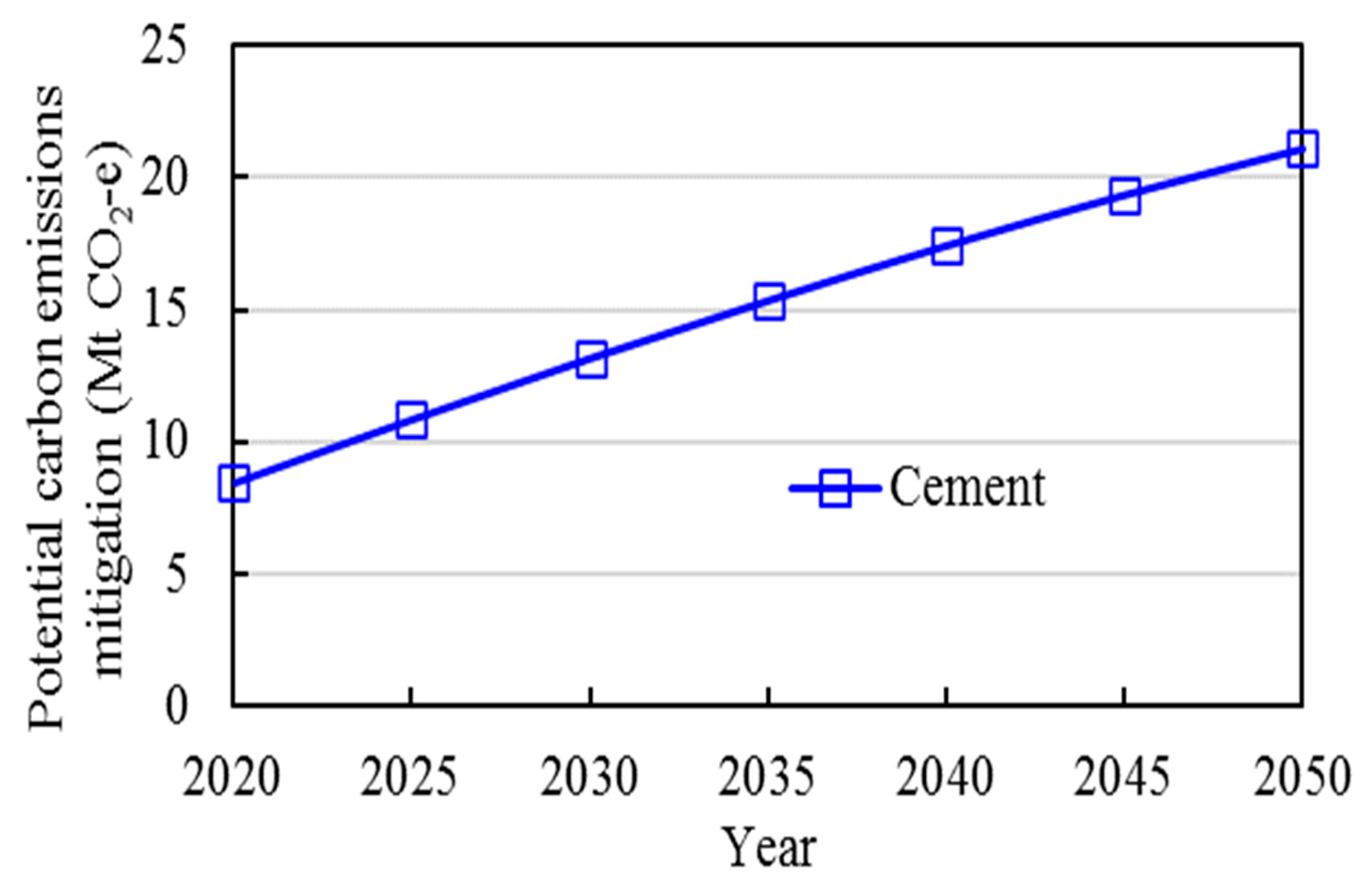
Figure 22.
Mitigation status of carbon emissions by 2030 and 2050.
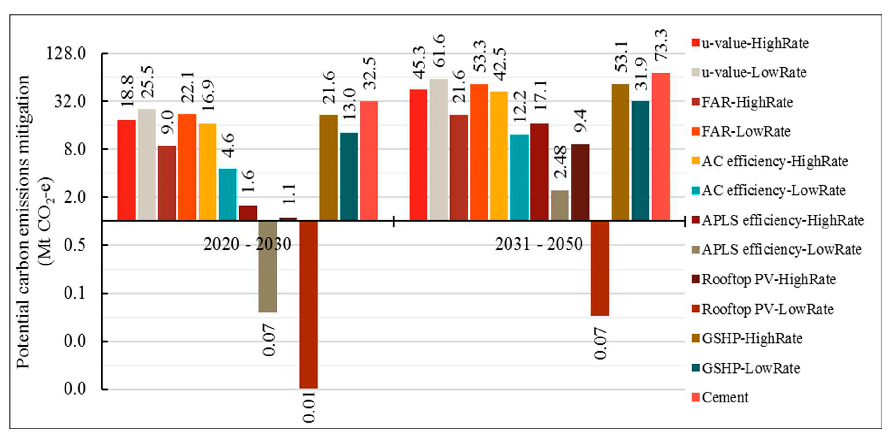
Figure 23.
Potential mitigation of carbon emissions based on integrated scenarios.
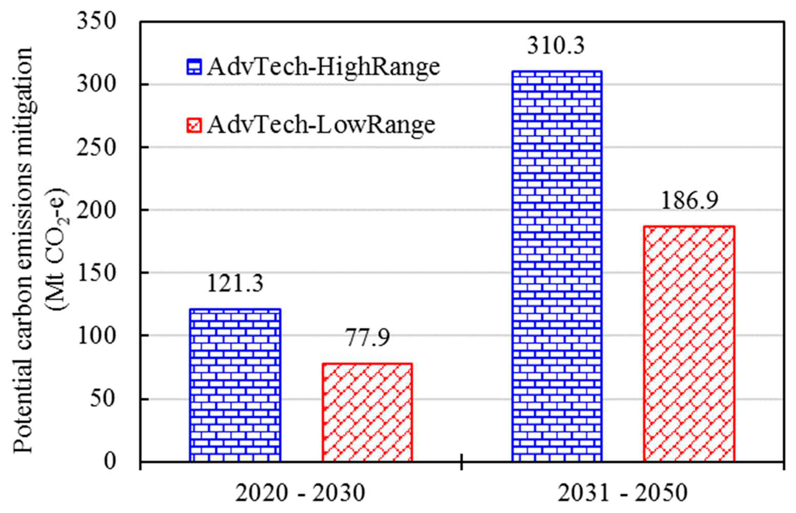
Figure 24.
Status of total final energy for residential cooling.
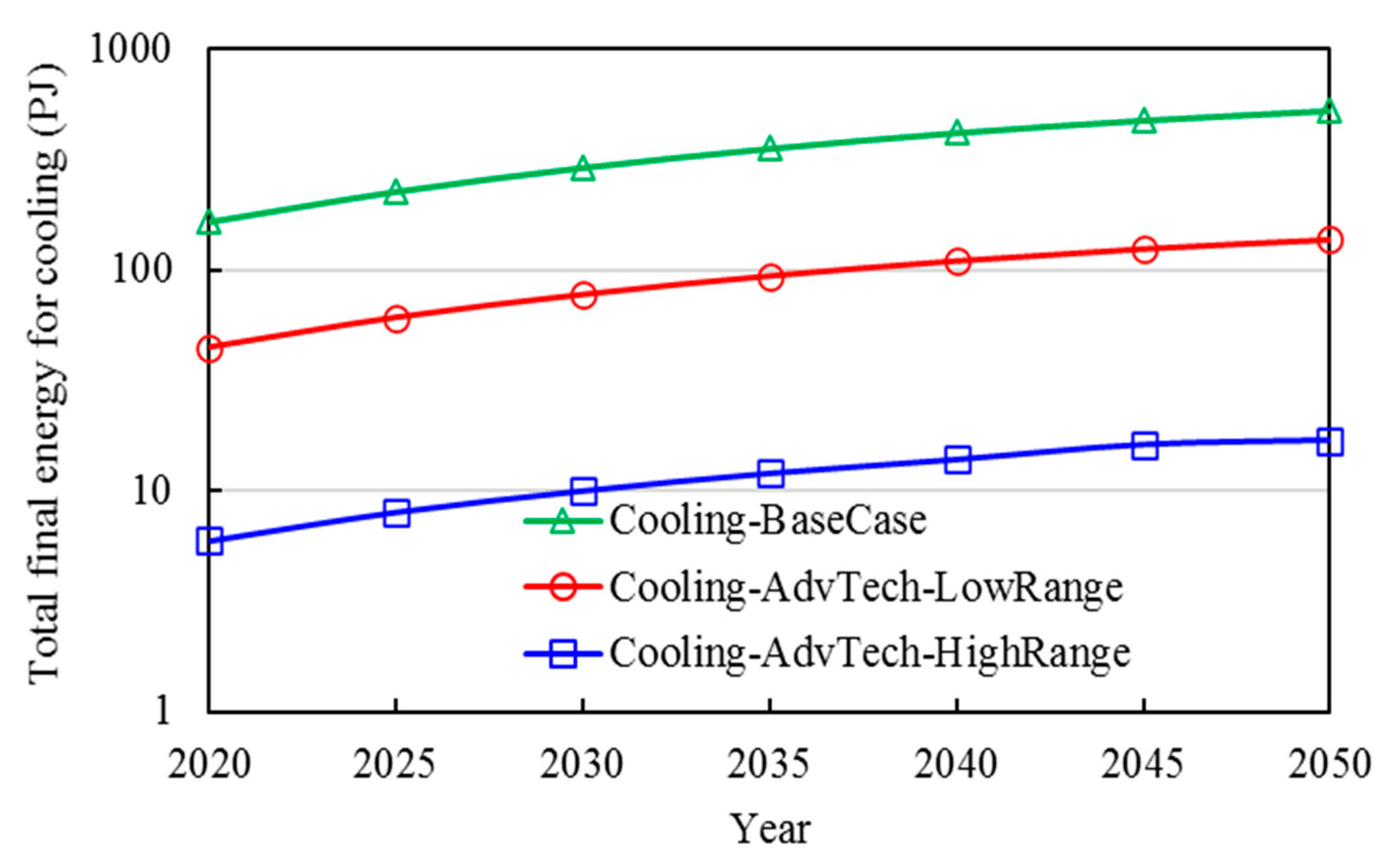
Figure 25.
Status of total final energy for residential appliances (APLs).
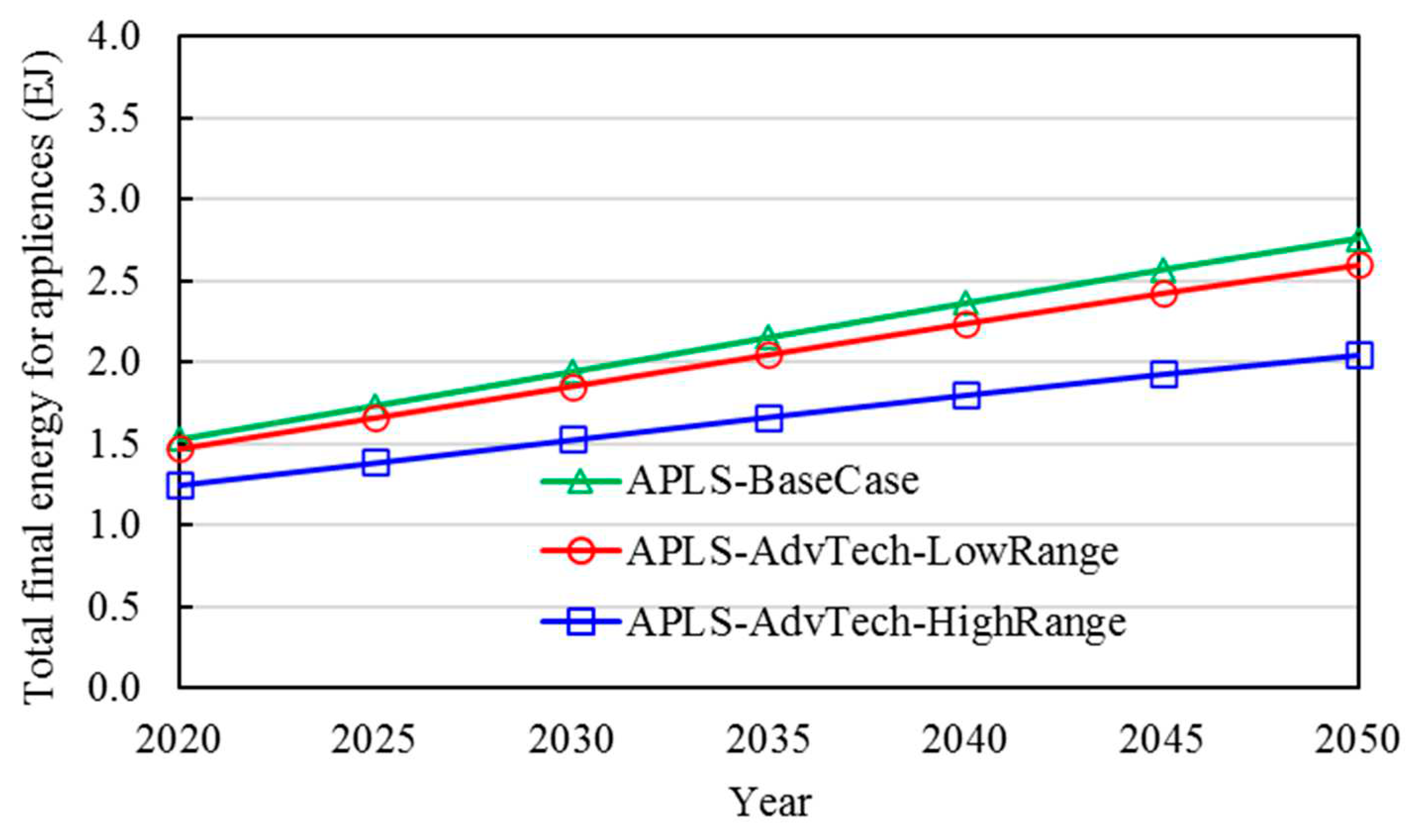
Figure 26.
Status of building floor space per capita.
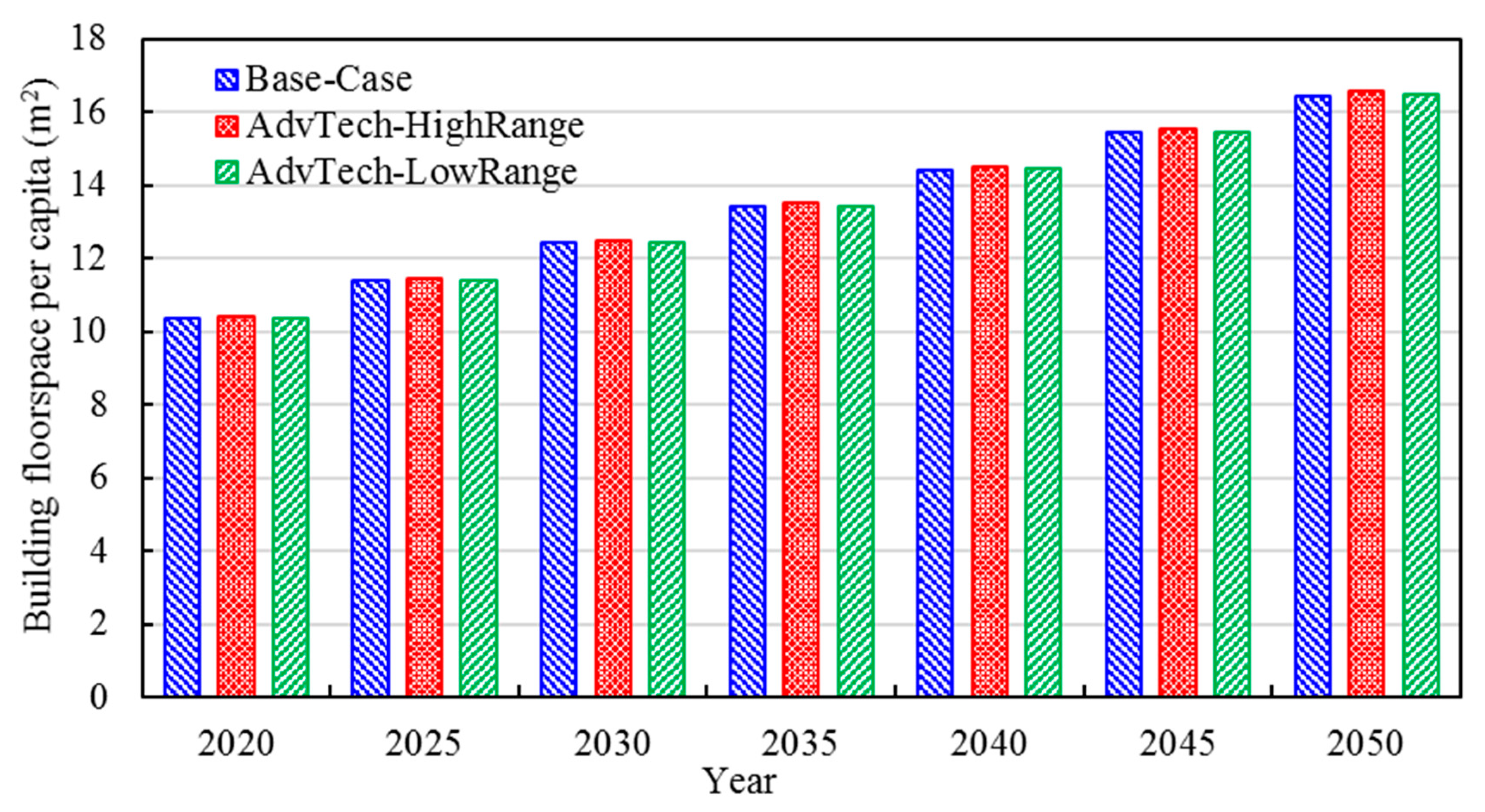
Figure 27.
Status of total building floorspace.
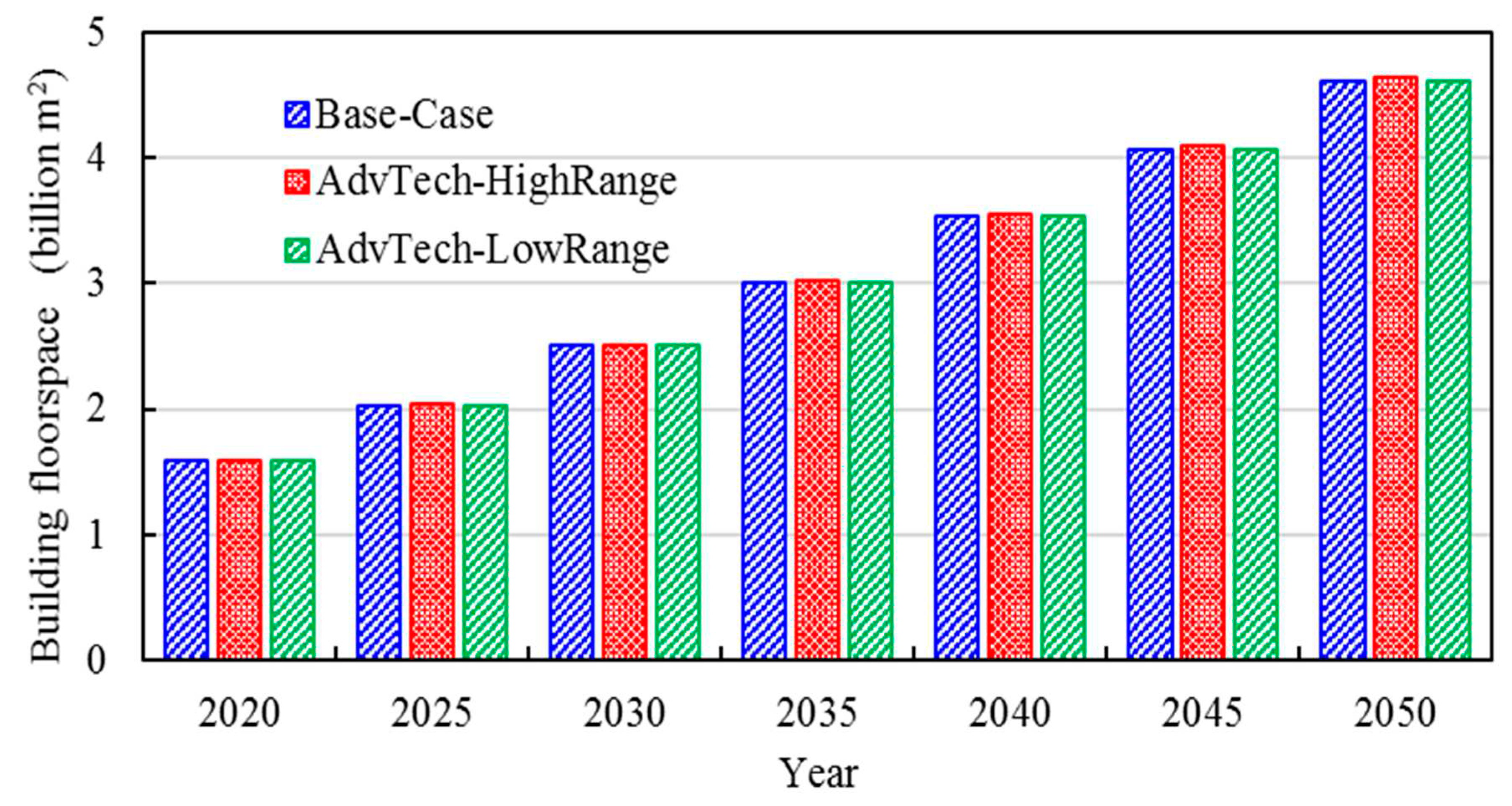
Figure 28.
Potential mitigation of carbon emissions based on AdvTech-HighRange.
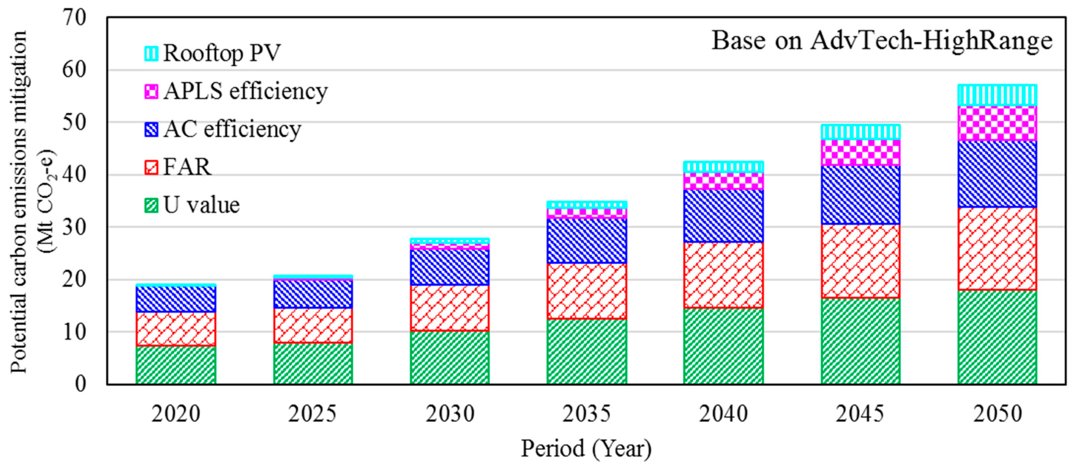
Figure 29.
Potential mitigation of carbon emissions based on AdvTech-LowRange.
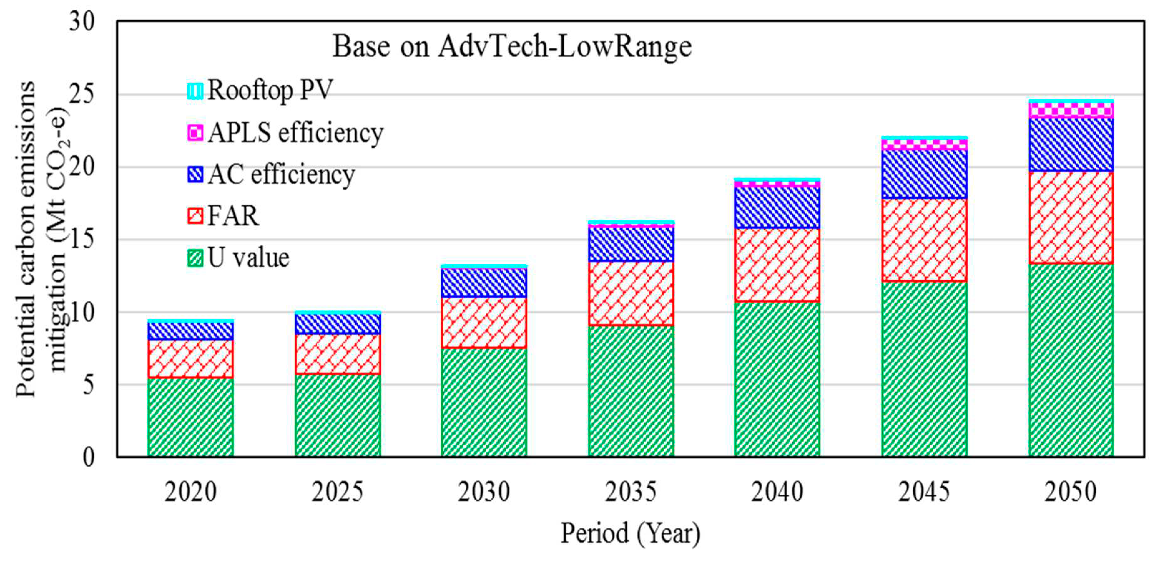
Figure 30.
Contribution to mitigate carbon emissions based on AdvTech-HighRange.

Figure 31.
Contribution to mitigate carbon emissions based on AdvTech-LowRange.
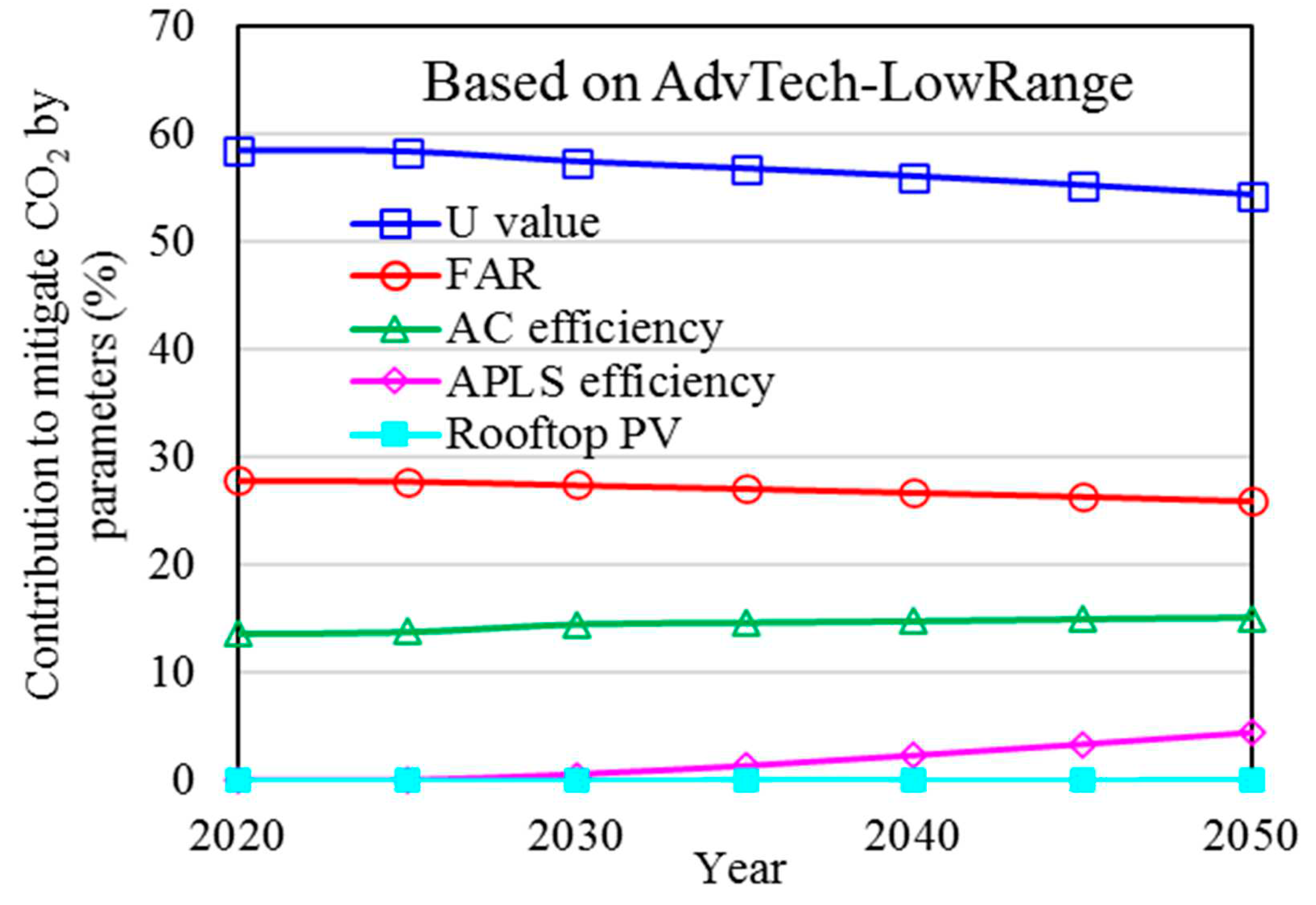
Figure 32.
Potential mitigation of carbon emissions based on AdvTech-HighRange.
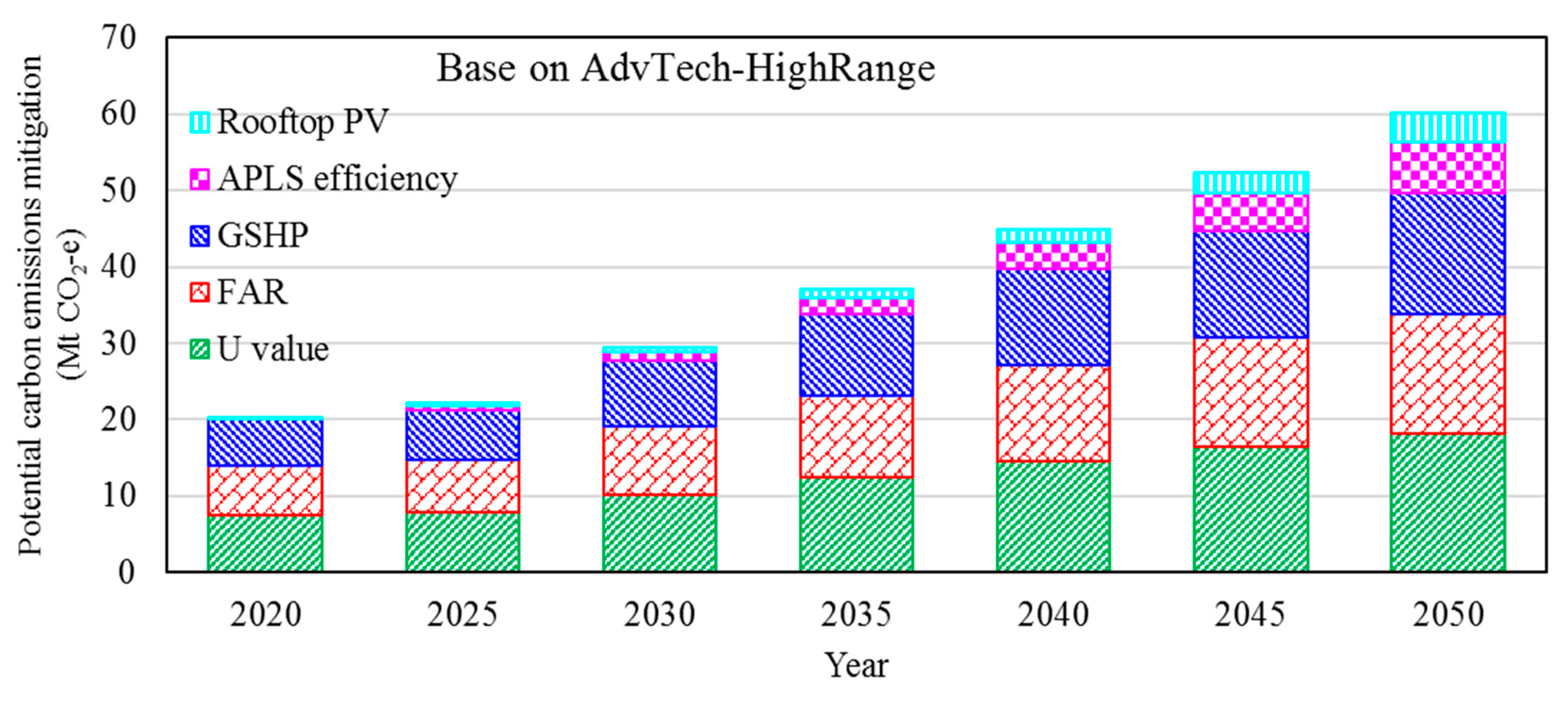
Figure 33.
Potential mitigation of carbon emissions based on AdvTech-LowRange.
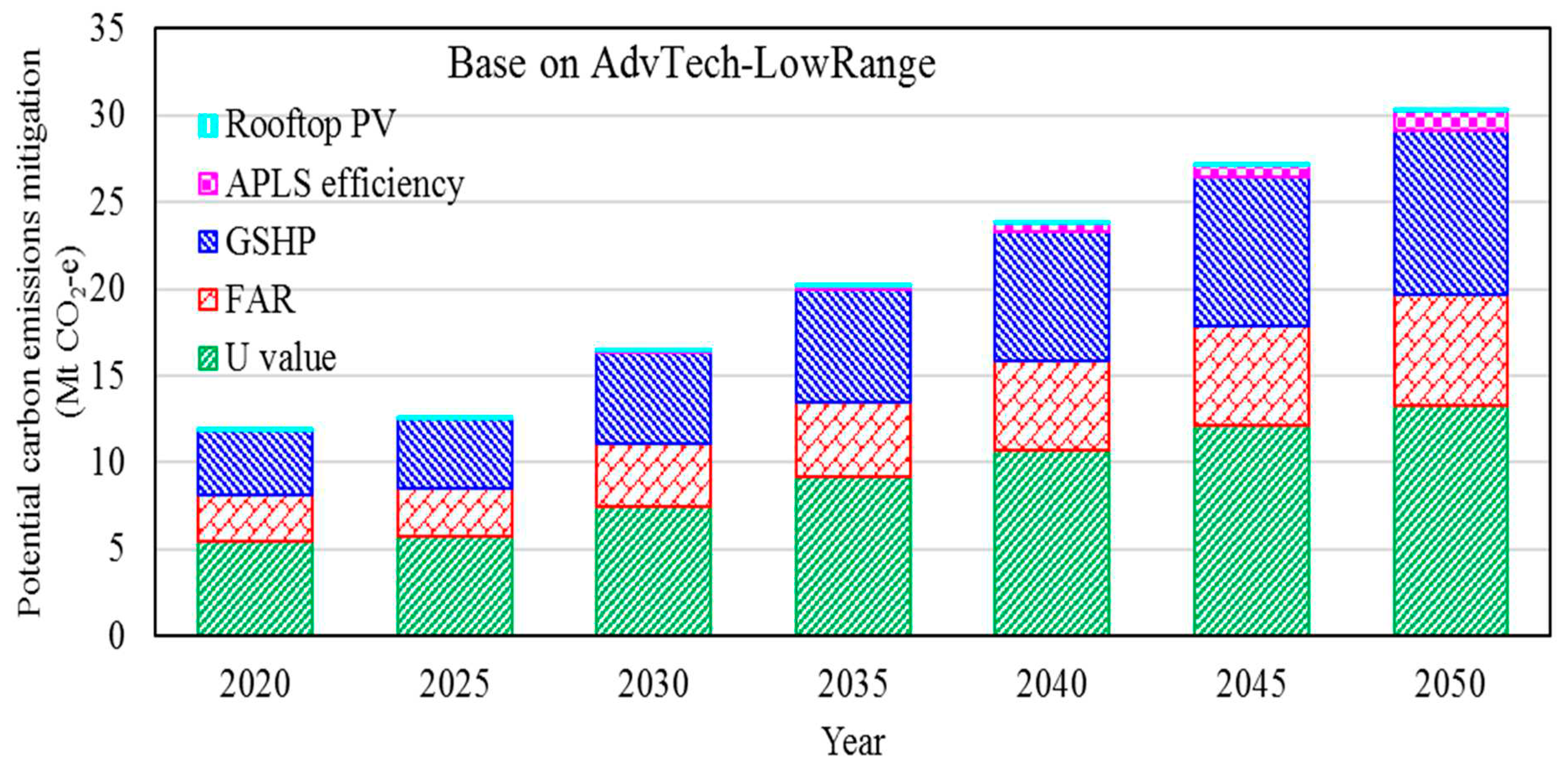
Figure 34.
Contribution to mitigate carbon emissions based on AdvTech-HighRange.
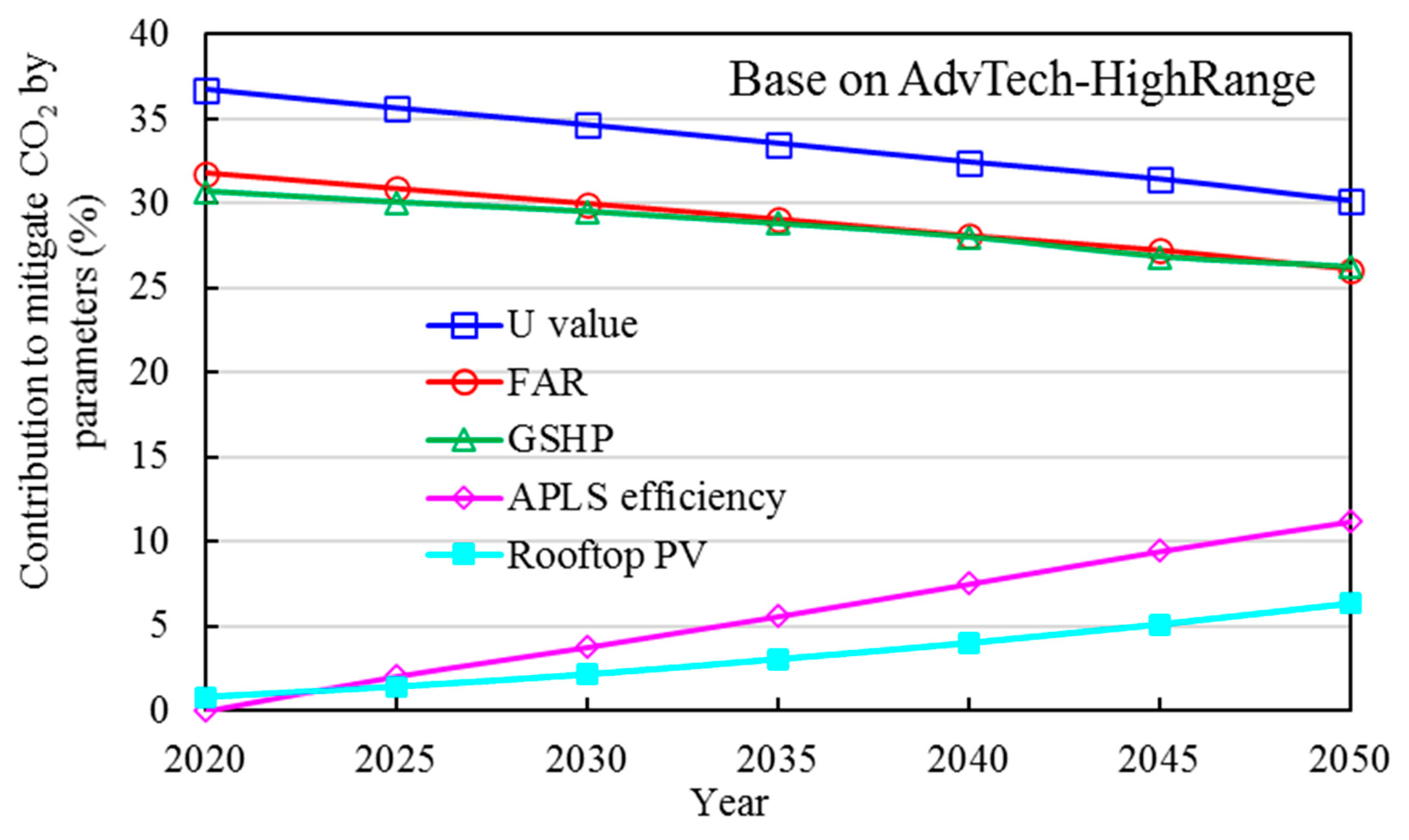
Figure 35.
Contribution to mitigate carbon emissions based on AdvTech-HighRange.
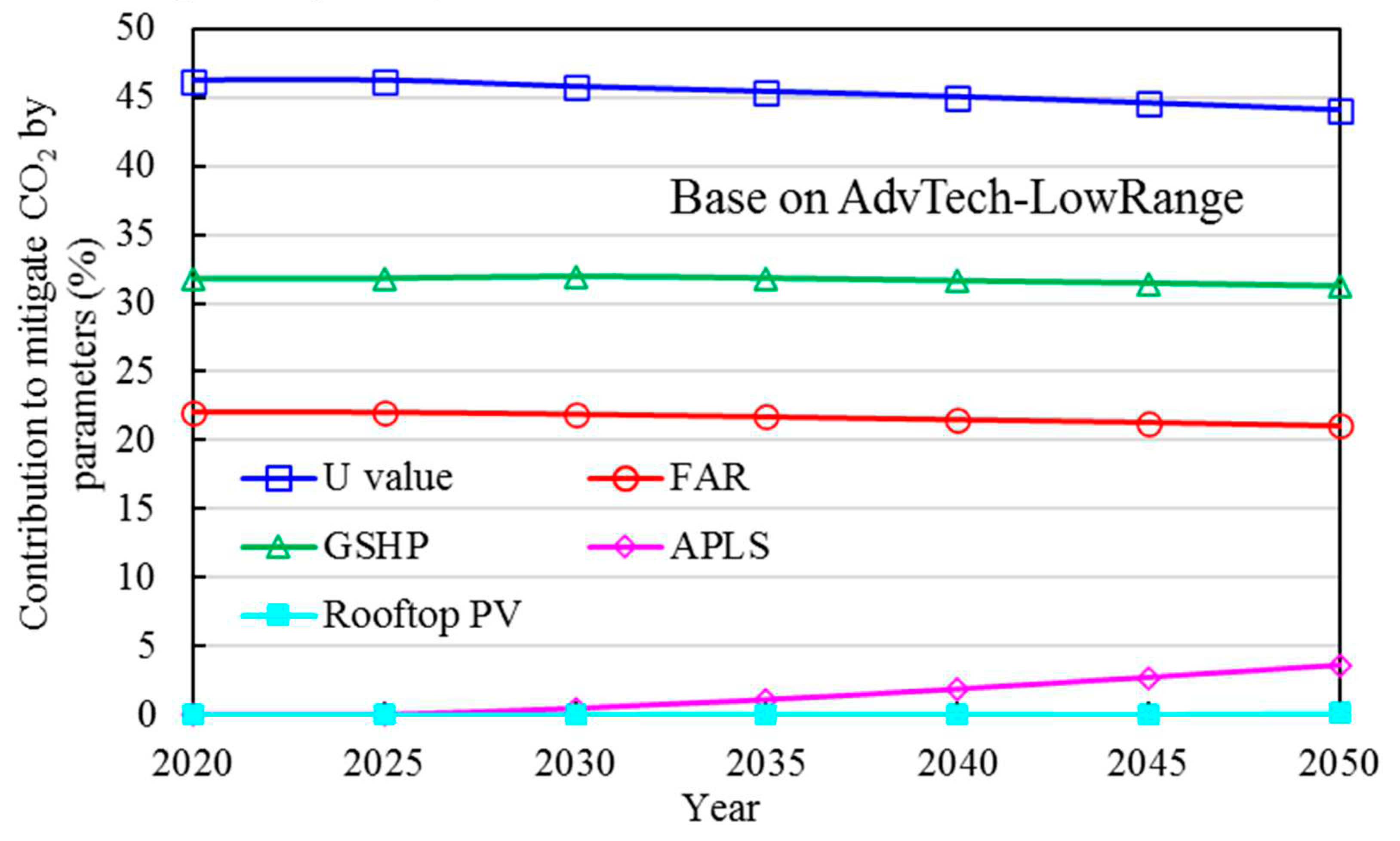
Figure 36.
Status of carbon reduction, ambition gap, and mitigation gap with 1.5˚C scenario.
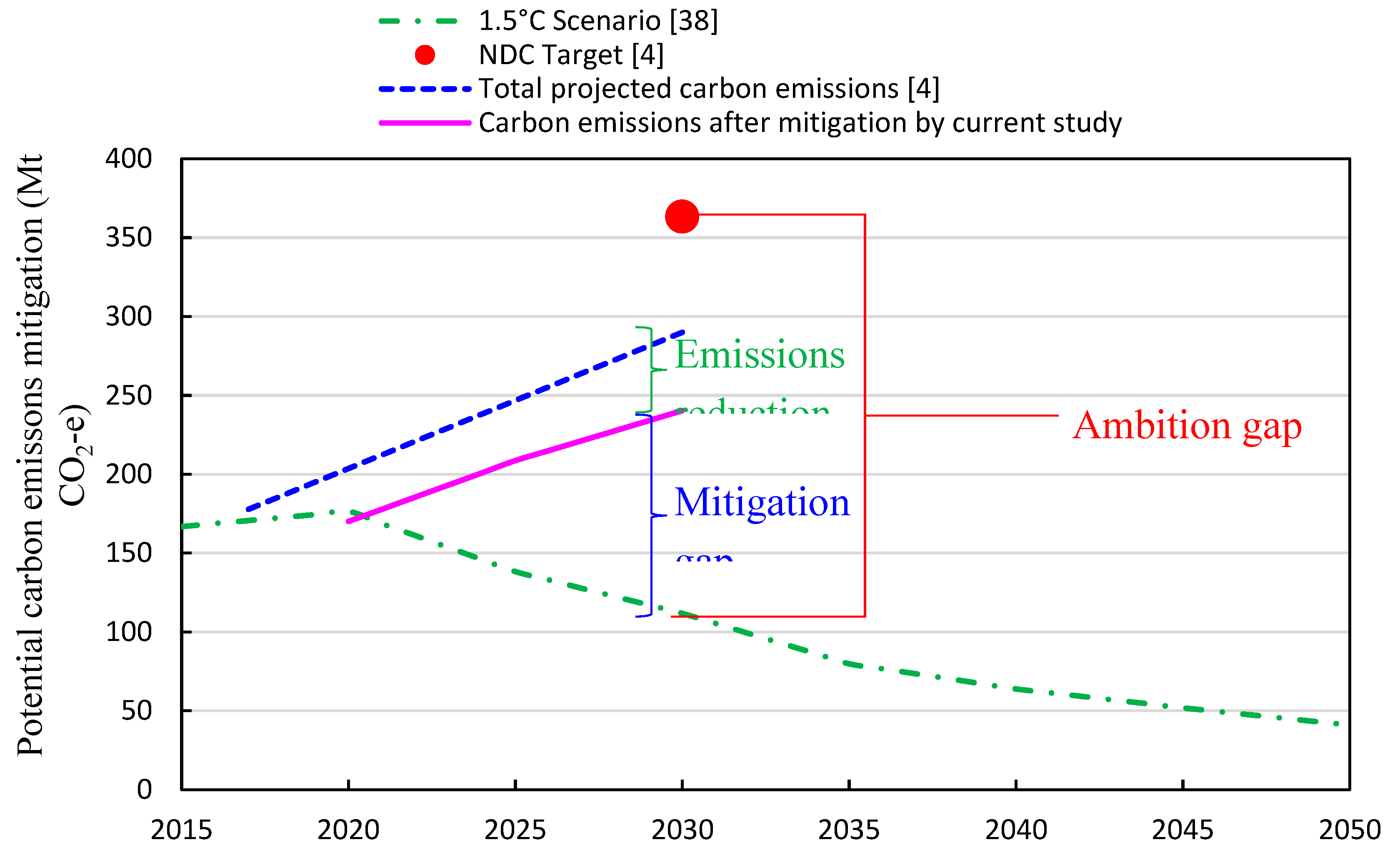
Table 1.
Scenario’s analysis of this study.
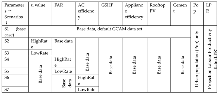
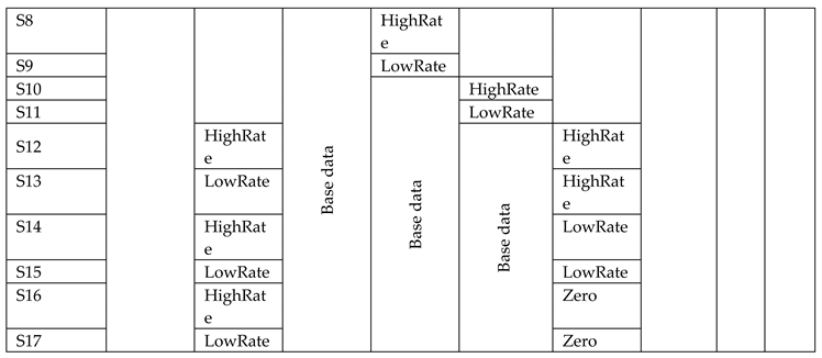
Table 2.
Integrated scenario’s based on technology ranges.
| Individual scenario | Variable rate | Integrated scenario |
| U value (S3) FAR (S5) |
Low | AdvTech-HighRange |
| AC Efficiency (S6) GSHP (S8) APLs Efficiency (S10) Rooftop PV (S12) Cement (S1) |
High | |
| High (FAR-High) Base | ||
| U value (S2) FAR (S4) |
High | AdvTech-LowRange |
| AC Efficiency (S7) GSHP (S9) APLs Efficiency (S11) Rooftop PV (S15) |
Low | |
| Low (FAR-Low) | ||
| Cement (S1) | Base |
Disclaimer/Publisher’s Note: The statements, opinions and data contained in all publications are solely those of the individual author(s) and contributor(s) and not of MDPI and/or the editor(s). MDPI and/or the editor(s) disclaim responsibility for any injury to people or property resulting from any ideas, methods, instructions or products referred to in the content. |
© 2023 by the authors. Licensee MDPI, Basel, Switzerland. This article is an open access article distributed under the terms and conditions of the Creative Commons Attribution (CC BY) license (https://creativecommons.org/licenses/by/4.0/).
Copyright: This open access article is published under a Creative Commons CC BY 4.0 license, which permit the free download, distribution, and reuse, provided that the author and preprint are cited in any reuse.


