Submitted:
03 October 2023
Posted:
09 October 2023
You are already at the latest version
Abstract
Switched model predictive control (S-MPC) and recurrent neural network with long short-term memory (RNN-LSTM) are powerful control methods that have been extensively studied for energy management in microgrids (MGs). These methods are complementary in terms of constraint satisfaction, computational demand, adaptability, and comprehensibility, but typically one method is chosen over the other. The S-MPC method selects optimal models and control strategies dynamically based on the system’s operating mode and performance objectives. On the other hand, integration of auto-regressive (AR) with these powerful control methods improves prediction accuracy and system conditions’ adaptability. This paper compares the two approaches to control and proposes a novel algorithm called Switched Auto-regressive Neural Control (S-ANC) that combines their respective strengths. Using a control formulation equivalent to S-MPC and the same controller model for learning, the results indicate that pure RNN-LSTM cannot provide constraint satisfaction. The novel S-ANC algorithm can satisfy constraints and deliver comparable performance to MPC while enabling continuous learning. Results indicate that S-MPC optimization increases power flows within the MG, resulting in efficient utilization of energy resources. By merging the AR and LSTM, the model’s computational time decreased by nearly 47.2%. Also, this study evaluated our predictive model’s accuracy: (i) R-squared error is 0.951, indicating strong predictive ability, and (ii) mean absolute error (MAE) and mean square error (MSE) values of 0.571 indicate accurate predictions with minimal deviations from actual values.
Keywords:
auto-regressive
; control and optimization
; energy management
; recurrent neural network
; long short-term memory
; microgrid
; switched model predictive control
1. Introduction
Model predictive control (MPC) is a control approach widely utilized in many industries, including chemical, electrical, and mechanical engineering. It is well-suited for microgrids (MGs) because it deals with restrictions and optimizes performance over time [1,2,3]. MPC entails formulating and solving an optimization problem at each time step to determine the optimal control inputs for the next step. A MPC is described in [4] for effective MG optimization, and mixed integer linear programming (MILP) is employed to solve the problem posed. MPC-inspired energy management (EM) system employed a neuro-fuzzy method that accounts for renewable energy sources (RESs)’ intermittent nature in grid-connected MG with loads and photovoltaic (PV) reported in [5]. [6] presents scenario-based stochastic programming with a rolling horizon strategy for minimizing the operating expenses of MGs when wind speed is unknown. The rolling horizon or MPC techniques are reactive-based methodologies that modify or update data from deterministic approaches. A scenario-based MPC was developed in [7] to reduce operating expenses and overall emissions. To achieve inexpensive and flexible operation, [8] provides MPC-based optimum management for renewable energy MGs with hybrid energy storage systems (ESSs), such as hydrogen, batteries, and capacitors. A hierarchical MPC-based technique for islanded AC MG addressed power quality and unbalanced power-sharing difficulties [9]. Despite this, traditional MPC cannot control the MG in various operational modes.
In contrast, Switched Model Predictive Control (S-MPC) is a variant of MPC that employs multiple models, each representing a unique mode of operation or scenario of the system. S-MPC selects the optimal model and associated control strategy based on the current system state and desired performance goals. This makes it possible for S-MPC to handle systems with mode-dependent dynamics. MPC is distinguished from S-MPC by using a single model to predict the system’s future behaviour [10]. S-MPC employs multiple models and switches between them based on the system’s current state. S-MPC can provide greater performance and robustness than MPC, especially for complex systems with multiple modes or operating conditions [11,12]. In another study, a novel study presents a hybrid MG model that incorporates two switched receding horizon control laws. This strategy mitigates overall energy expenses and maximizes the efficient utilization of RESs for expansive business establishments while accommodating fluctuations in grid connectivity circumstances [13]. Also, [14] outlines the process of designing and applying a S-MPC to wind turbine systems, intending to manage the intricate nature and nonlinearity inherent in wind turbine systems. The system employs qpOASES as an integrated solver for online optimum control. It incorporates a cyber-physical real-time emulator for utility-scale wind turbines with variable-speed and variable-pitch capabilities. This study showcases the viability and efficacy of S-MPC in attaining control objectives for Wind turbine systems in real-time, utilizing brief control periods. In addition, in [15] study presents a novel technique to enhance wind turbine control by introducing a S-MPC framework. The proposed approach aims to solve the limitations of the conventional continuous control-based MPC algorithm. The results of the comparative analysis indicate that the proposed algorithm exhibits superior performance compared to the existing MPC in various aspects, including computational efficiency, load mitigation, and dynamic response. [16] presents a novel S-MPC method specifically tailored for discrete-time nonlinear systems. The simulation outcomes emphasize its superiority over a conventional MPC technique regarding computational efficacy and control effectiveness. Another study presents a novel S-MPC methodology for power converters. During transient periods, the system utilizes horizon-one nonlinear finite control set MPC to steer the system towards the intended reference [17].
On the other hand, S-MPC’s performance is highly vulnerable to model mismatch. In other words, it must select a suitable system model. Furthermore, the rising complexity of S-MPC impacts the stability and maintainability of MG control [18,19]. These challenges lead to the accuracy issue in S-MPC methods. In addition, the computational time of S-MPC is much higher because of the prediction horizon and several steps. Many authors have studied machine learning (ML) techniques to increase the accuracy of the MG system.
To improve scheduling effectiveness in networked microgrids (NMGs), with the main goal of minimizing the effects of electricity outages. The paper presents a framework consisting of three stages to evaluate power transactions, manage renewable energy and market price risks, and tackle uncertainties. This framework is formulated as a mixed-integer linear programming problem [20]. On the other hand, [21] introduces a novel approach utilizing the Internet of Things (IoT) to optimize and regulate power loads in citizen energy communities dynamically. This technique is compared to the conventional Direct Load Control (DLC) method. This technique aims to enhance power use efficiency through programmable appliances and dynamic demand response. Simulations have demonstrated potential reductions in energy bills, lower reliance on flexible energy sources, reduced interruptions, and increased peak-to-average ratio (PAR). In order to model the behaviour of RESs, such as wind and solar, an auto-regressive moving-average (ARMA)-based scenario generation has been implemented. Large industries will receive direct assistance from storage and demand-side management systems to reduce energy costs [22]. The other work employs an ARMA model to forecast solar PV, wind power generation, and electricity demand. Second, an optimal generation scheduling procedure is intended to reduce system operating expenses. The simulation results indicate that optimal generation scheduling can minimize operating expenses under the worst-case scenario [23]. In [24] study, combining two models, the ARMA and the Nonlinear Auto Regressive with exogenous input (NARX), a novel method was presented for predicting solar radiation. This decision was made to utilize the benefits of both models to produce more accurate prediction results. Simulation results have validated this hybrid model’s ability to predict weekly solar radiation averages. Although these previous solar radiation forecasting techniques, particularly ARMA models, are effective for particular uses, they are unsuitable for others requiring high forecasting precision. Several researchers have proposed hybrid models to improve the precision of solar radiation forecasting. Moreover, there is still a proper plant model and prediction horizon, so the computational time of the model is still so high [24].
There are numerous studies on ML methods rather than AR models. For instance, [25] thoroughly investigated the predicting performance of several recurrent neural network (RNNs) designs, such as a long short-term memory (LSTM), gated recurrent unit (GRU), and bidirectional LSTM. Using local weather forecasts and historical weather data, [26] proposed a LSTM-based next-day forecasting model of hourly global horizontal irradiance (GHI). [27] and [28] suggested LSTM-based models with only the next day’s weather forecasts as input. Studies by [29] and [30] use similar LSTM-based techniques. [31,32] validated the performance of hybrid deep learning models built on convolutional neural networks (CNNs) and LSTM for day-ahead GHI forecasting. In addition to RNN-based approaches, there are studies evaluating the performance of other statistical and ML models for solar irradiance forecasting, such as coupled AR and dynamic system by [33], Markov switch model [34], and support vector machine (SVM) by [35]. [36] reported an LSTM-based model for hour-ahead solar irradiance forecasting. The input, which included historical GHI and meteorological data from the preceding 24 hours, was utilized to forecast the GHI for the next hour [36]. The results reveal that the LSTM-based model outperforms other models, such as auto-regressive integrated moving average (ARIMA) and CNN [36]. [37] investigated the performance of LSTM and GRU. [38] and [39] published hybrid CNN-LSTM models for hour-ahead GHI forecasting. This study showed that incorporating external weather information considerably increases prediction accuracy. Unlike day-ahead irradiance forecasting methods, hour-ahead forecasting algorithms create projections for the following hour using only historical data.
On the other hand, RNNs are a form of ML technology widely employed for time series prediction and modelling dynamic systems [40,41]. RNNs are an artificial neural network (ANN) that is particularly useful for modelling time-series data and may be used to anticipate future MG behaviour [42,43]. RNNs may learn and adapt to system dynamics by learning the temporal dependencies in the data. RNNs have been used to solve various MG control challenges, including load forecasting, renewable energy integration, and demand response management [44,45,46]. RNNs have been applied to various systems, including power systems [47,48], with promising prediction accuracy and flexibility results.
In summary, both control families have benefits and drawbacks, and their complementarity is evident. On the one hand, S-MPC struggles with system complexity and long-term prediction horizons, whereas the combination of AR and LSTM (AR-LSTM) can deal with complex systems and infinite prediction horizons naturally. AR-LSTM, conversely, is challenging to satisfy constraints and lacks interpretability, whereas S-MPC can provide safety guarantees and understandability.
Although there is a clear potential for synergy between the two families of methods, there have been few attempts to combine their relative advantages. This research deficiency is not limited to applying EM for MG. Control and ML communities evolve independently, adopting radically different notations to formulate the same problem. In spite of the parallel developments, several authors [49,50,51] have suggested that a collaboration between the two groups could result in potential advantages. Combining these methodologies is a powerful method of integrating robust control theory methods with ML approaches to exploit additional information from real-time data [52,53].
As shown in Table 1, each control method has strengths and limitations. MPC and S-MPC offer robust optimality and constraint handling but may have computational challenges. AR and RNN-LSTM are efficient in computation but may not manage complex constraints effectively. S-ANC combines AR models with neural control, balancing optimality and computational efficiency. The choice of control method depends on the specific application and trade-offs between these criteria.
1.1. Contributions and Research Questions
This paper is motivated by how AR-LSTM and S-MPC can collaborate in applying EM of MG. While there is a consensus that combining the two algorithms may yield benefits, little has been done to develop methods that involve the two algorithms working together. In addition, the works investigate how these controllers can collaborate with the algorithms working at different control designs and modes. No previous research has compared and combined S-MPC and AR-LSTM for the same optimal control problem formulation in EM for MG.
The second objective of this paper is to propose a novel method known as Switched Auto-regressive Neural Control (S-ANC), which merges S-MPC and AR-LSTM synergistically. The development and formulation of this new S-ANC algorithm are motivated by the conceptual and practical comparison of S-MPC and AR-LSTM. In contrast to comparable approaches, our method combines the S-MPC objective function and constraints and the AR-LSTM optimization and prediction function. This practice ensures interoperability between the two methods and enables the truncation of the S-MPC optimization problem, which can become highly complex even for relatively simple MG structures. Finally, the flexible hybrid MG case describes and evaluates this new algorithm.
Consequently, the primary contribution of this paper is the introduction of S-ANC, a control algorithm that combines techniques from the communities of control theory and ML. This algorithm is evaluated, and a new standard framework is generated for EM of hybrid MG. In addition, the proposed S-ANC algorithm applies to various applications and domains, such as complex industrial processes and energy markets. This study also combines control theory and ML by comparing and disentangling the key distinctions between S-MPC and AR-LSTM.
2. Identifying the distinctions between S-MPC and AR-RNN-LSTM
Optimal control determines the actions that optimize a performance objective by solving a sequential decision-making problem. The preceding section highlighted the need for comparing S-MPC and AR-LSTM, the two primary approaches for optimal control applied to EM for hybrid MG control, and the possibility of combining them. Both methods utilize some components, while others are more controller-specific. These formulation differences make it difficult to compare and combine the two approaches, necessitating a conceptual analysis. It assists in identifying the primary methods for optimal control and establishes a common ground for a comprehensive classification. The sections that follow detail the most important aspects of these control methods.
2.1. Strategy
There are typically two ways to approach an optimal control problem: by employing the S-MPC-inherent receding horizon principle or formalizing the problem as an AR-LSTM.
S-MPC is a control strategy that involves using a mathematical model of the system being controlled to predict the system’s future behaviour and optimize a control signal over a finite time horizon. At each time step, the control signal is updated based on the current state of the system and the predictions made by the model. It is widely used in industrial control applications, such as process control, automotive control, and robotics, where it is important to consider the system’s dynamics being controlled and optimize performance over a prediction horizon. At each time step k in S-MPC, switching logic controls multi-mode for the accumulators that fully describe the controller model at the current time. Then, the trajectories of the future state x and input u are optimized for a prediction horizon based on the explicit representation of an objective function J and a controller model F. J is the minimization of the imported energy and maximization of the exported energy. The constraints H are also introduced explicitly in the optimization problem. Objective function, model, and constraints may also depend on model outputs y and time-invariant parameters p. In addition, is the reference variable representing the PV, load data, and zero along the prediction horizon . and are weighting coefficient reflecting the relative significance of and penalizing relatively large variation in , respectively. Implemented is only the initial control input from the optimized trajectory [11]. Figure 1 depicts the full S-MPC procedure.
In the application of S-MPC to EM for MGs, the state vector x represents the state of charge of the accumulators (), such as the battery, fuel tank, and water tank, and the model output y illustrates the imported and exported energy, such as a grid to the load and PV to the grid, and the battery ( + ). Depending on whether or not the controller model employs physical insights, the set of time-invariant parameters p may or may not represent the physical properties of the MG.
In contrast to RNN-LSTM, AR models are not neural network architectures. On the contrary, they are statistical models that identify dependencies and patterns within a time series based on its own lagged values. The AR model predicts the future values of a variable based on its historical values and the estimated coefficients during model training. In other words, AR models are a statistical modelling technique that assumes a variable’s current value is a function of its previous values. They are utilized frequently for time series analysis and forecasting. Therefore, AR models can be viewed as linear regression in which the predictors are the values of the same variable at a prior time [24]. AR models can be used to model the system’s dynamics within the context of control systems or reinforcement learning. The model can predict future states or observations by estimating the AR coefficients. These predictions can then be fed into control algorithms or reinforcement learning agents in order to optimize control signals or decision-making. Unlike neural network architectures, AR models are not adaptive by nature. The estimation of AR coefficients requires training on historical data, and their performance may degrade if the underlying dynamics of the system change significantly over time.
The following equation can mathematically represent an AR model of order q [24]:
where represents the value of the time series at time k in this equation. c is a constant term or an intercept. terms represent AR model coefficients. The coefficients or weights associated with the previous values of the time series are denoted by 1, 2, ⋯, q. , , ⋯, represent the lagged values of the time series at time points , , ⋯, , respectively. is the error term or random noise at time k, representing the data portion the model cannot explain.
RNN-LSTM is a neural network type ideally suited for processing sequential data. Unlike feed-forward neural networks, it has loops that allow information to be passed from one sequence step to the next. The approach for employing RNN-LSTM includes selecting an appropriate network architecture, an optimization algorithm for training the network, and an appropriate set of hyper-parameters. RNN-LSTM is an extension of a feed-forward neural network with internal memory. RNN-LSTM is recurrent because it performs the same function for each data input, while the output of the current input is dependent on the previous computation. After the output has been generated, it is duplicated and sent back into the recurrent network [61]. For decision-making, it considers both the current input and the output from the previous input it learned. As shown in Figure 1, the input vector of an LSTM network is at time step k. represents the output vectors passed through the network between time steps k and . Three gates update and control the cell states in an LSTM network: the forget gate, input gate, and output gate. The gates are activated by hyperbolic tangent and sigmoid functions. Given new information that has entered the network, the forget gate determines which cell state information to forget. Given new input information, the input gate determines what new information will be encoded into the cell state. Using the output vector , the output gate controls what information encoded in the cell state is sent to the network as input in the subsequent time step.
In the mathematical modelling of RNN-LSTM, the current state can be expressed mathematically as:
where represents the current state, represents the previous state, and is the current input. Because the input neuron would have applied the transformations to the previous input, we now have a state of the previous input rather than the input itself. Each successive input is, therefore, referred to as a time step.
Considering the simplest form of a RNN-LSTM, where the activation function is tanx, the weight at the recurrent neuron is , and the weight at the input neuron is , we can write the equation for the state at time k as follows [61]:
In this instance, the recurrent neuron only considers the previous state. The equation may involve multiple such states for longer sequences. After calculating the final state, the output can be generated. Once the current state has been computed, we can then calculate the output state as follows [61]:
where is the output state and is the weight at the output state. This process is represented by Figure 2.
First, it extracts from the input sequence and then outputs , which, along with , is the input for the subsequent step. Therefore, and are the inputs for the subsequent step. Similarly, from the subsequent step is the input for for the subsequent step, and so on. Consequently, it remembers the context throughout training.
A cost function quantifies "how well" a neural network performs with respect to the training sample and the expected output. It may also depend on factors like weights and biases. This is a single value, not a vector because it evaluates the overall performance of the neural network. The objective of the cost function is to evaluate the network’s performance to minimize its value during training. The cost function for a typical RNN-LSTM is the sum of losses at each time step [62].
where represents the parameters of the RNN, T represents the length of the input sequence, represents the predicted output and represents the actual output at time step k. L is the loss function quantifying the difference between the predicted and actual output. The RNN’s training parameters are adjusted to minimize the cost function using gradient descent or a comparable optimisation algorithm. The objective is to identify the parameters that minimize the loss over all time steps, resulting in an RNN that can accurately predict the output for a given input sequence.
2.2. Problem-solving method
By analyzing the control processes illustrated in Figure 1a,b, it is possible to identify a number of expressions with total or partial equivalence between the two methods.
S-MPC can be solved implicitly by performing switching logic, forecasting, and resolving a dynamic optimization problem at each time step or explicitly by learning a control policy from data generated by a S-MPC with any function approximation. Consequently, S-MPC has a higher online computational cost because every control step requires estimation of the states and dynamic optimization. Typically, the optimization problem in S-MPC is solved using numerical optimization techniques, such as nonlinear programming or quadratic programming (QP) (in this paper, QP has been used), to solve the optimization problem. The solution to the optimization problem over the prediction horizon provides the optimal control signal. At each time step, the first component of the optimal control signal is applied to the system, and the process is repeated with updated state and prediction horizon values. S-MPC necessitates the solution of an optimization problem at each time step, which can be computationally expensive for large systems.
The training process for AR-LSTM involves back-propagation through time (BPTT), a variation of the back-propagation algorithm that considers temporal dependencies in the data. The RNN is unrolled throughout the training for a predetermined number of time steps, and gradients are calculated at each step. The RNN’s weights are then updated based on the gradients accumulated across all time steps. The most prevalent optimization algorithm for training RNNs is gradient descent, which involves updating the weights iteratively in the direction of the loss function’s negative gradient [61]. However, the standard gradient descent algorithm is susceptible to issues such as vanishing gradients, in which the gradients become extremely small and the weights do not update. Several variants of gradient descent, such as the adaptive gradient descent algorithms AdaGrad, RMSProp, and Adam, have been developed to address this issue [63].
2.3. Peak Performance
In S-MPC, the quality of the optimization solution depends on the controller model’s precision, which is frequently simplified for computational purposes. Stability and practicability are intrinsically assured for S-MPC, whereas there is only an immature theory for these issues in AR-LSTM [64]. The absence of safety guarantees in AR-LSTM results from the constraints not being imposed directly in the formulation of the solution method. The optimality of the S-MPC solution depends on the accuracy of the model used to predict the system’s behaviour and the optimization algorithm’s ability to find the optimization problem’s global optimum. If the model is inaccurate or the optimization algorithm fails to find the global optimum, the performance of the S-MPC controller may not be optimal.
The optimality of AR-LSTM relies on several factors, including the network’s architecture, the training optimization algorithm, and the complexity of the task being performed. AR-LSTM is capable of achieving high levels of performance on a wide variety of sequential data processing tasks, such as language modelling, machine translation, and speech recognition. AR-LSTM is able to model complex temporal dependencies in sequential data, which is one of its main advantages. The ability of AR-LSTM to incorporate feedback loops enables them to capture long-term dependencies that would be challenging to represent using other models, such as Gated Recurrent Unit (GRU). In addition, the ability to incorporate memory into the network via mechanisms improves the performance of RNNs on tasks requiring long-term memory. Nonetheless, several factors can restrict the optimality of AR-LSTM. One difficulty is the issue of vanishing and exploding gradients, which can hinder the network’s ability to discover long-term dependencies. This issue can be mitigated by employing specialized units, such as LSTM and GRU, and optimization algorithms designed to deal with these issues. Another issue is over-fitting, which can occur when the model becomes excessively complex and begins to fit the noise in the data rather than the underlying patterns. This can be remedied by employing regularisation techniques such as early stopping and dropout [65].
2.4. Calculational effort
S-MPC can require significant computational effort, especially for large-scale systems. S-MPC necessitates the solution of an optimization problem at each time step, which can be computationally costly. Moreover, a significant disadvantage of S-MPC is the need to solve an optimization problem online, which can be complex and involve many optimization variables. Consequently, controller models for S-MPC are commonly simplified at the expense of optimality, and gains in optimization solver efficiency are highly desired. Moreover, switching logic and prediction must be performed at each control step. Nonetheless, several techniques have been developed to reduce the computational effort required for S-MPC, such as online optimization and ML techniques that update the optimization problem as the system evolves.
The computational effort required for training and utilizing AR-LSTM can be substantial, especially for large-scale problems with many time steps and/or parameters. BPTT is the primary computational bottleneck because it is required to compute the gradients of the loss function with respect to the network parameters. Considering that the computational complexity of BPTT scales linearly with the number of time steps, training AR-LSTM on lengthy sequences can be computationally expensive. In addition, the number of network parameters can contribute to computational complexity, as larger networks require more computation to update weights during training and make predictions during inference. Several techniques have been developed to mitigate these computational challenges, including mini-batch training, which involves updating the weights based on a subset of the training data at each iteration, and gradient clipping, which involves capping the magnitude of gradients to prevent gradients from exploding during training [61].
3. Switched Auto-regressive Neural Control (S-ANC)
This section introduces the specifics of the novel S-ANC algorithm proposed. The objective is to learn from the architecture of RNN-LSTM while satisfying constraints. Switching logic, dynamic optimization, and learning are elements from the control and ML communities that are effectively combined to achieve this objective. First, Section 3.1 introduces the hybrid MG structure. Section 3.2 provides an overview of how S-MPC and AR-LSTM are merged logically. Then, Section 3.3 describes the S-ANC algorithm formally.
3.1. Hybrid MG description
This is a case study of a system constructed in Xanthi, Greece [66]. As depicted in Figure 3, the hybrid MG is comprised of a 15 kW PV array, a battery (BAT), a water tank (WT), and a fuel tank (FT) serving as energy storage systems (ESSs), an electrolyzer (EL), and a fuel cell (FC), as well as the utility grid (GR). The PV can be utilized on the hybrid MG as the primary energy source. If the PV cannot provide sufficient power, the BAT or the FC will meet the load. The GR will provide energy if the battery is depleted and no hydrogen is available. Alternatively, when the BAT is full and there is an excess, the EL will be utilized if there is space in the WT and the FT. The energy will then be sent to the GR.
3.2. Simple definition of the proposed method
To comprehend the intuition underlying S-ANC, one must first comprehend the distinctions between MPC and S-MPC to solve the QP and the two main learning methods of RNN: AR and LSTM. The S-MPC controller must be capable of selecting the appropriate model and control strategy based on the system’s current state, which necessitates additional computational resources and algorithmic complexity. In this paper, for instance, the system dynamics change significantly as the state of each accumulator in the hybrid MG changes; consequently, S-MPC can use different models for various states. This requires creating and validating multiple models, and the S-MPC controller must be able to switch between these models based on the current state.
The construction of S-MPC is challenging and intricate, particularly for the hybrid MG, which must accommodate many operating modes and complex switching conditions. The complexity is caused by a number of factors, including:
- Model development: The S-MPC necessitates the creation of multiple models that represent the system’s behavior in different operating modes. This requires an efficient system architecture and behavior.
- Mode detection: The S-MPC controller must be able to detect the current mode of operation of the system, which can be difficult in certain circumstances.
- Switching logic: The S-MPC controller must select the appropriate model and control strategy based on the current operating mode and desired performance objectives. This necessitates the design of switching logic that maps the system’s current state to the appropriate model and control strategy (a mode’s objective function and an operational mode’s objective function may differ).
The S-MPC solution method takes information from the hybrid MG, such as PV and load data and accumulator parameters, including their charging and discharging efficiencies. Then, the input u, state x, and output vectors y are defined. Based on the controller model, the objective function J is inferred at each control step using this method. After that, the state vector is converted to AR model in order to predict the value at the subsequent time step. It is a straightforward concept that can produce accurate forecasts for various time series problems. Nevertheless, the AR model needs the plant model and a prediction horizon, so the computational time of the model is still high. Therefore, the current state x, input u, and output vectors y are updated through the AR-LSTM method.
S-ANC employs time series values-based AR-LSTM to estimate the value of being in a particular output vector , as determined by S-MPC, with a prediction horizon of only one control step. By doing that, in S-ANC, the S-MPC method is truncated with the predicted output vector and optimized of the hybrid MG system during k steps ahead by employing the AR-LSTM method. Consequently, the principal components of the S-MPC, namely the reference, predictor, and switching logic, remain active in S-ANC; however, the time series value function is utilized to shorten the nonlinear program and enable learning. The interaction of S-ANC’s primary components is depicted in a diagram in Figure 4. The merging of S-MPC and AR-LSTM in the S-ANC algorithm is intuitively depicted in Figure 4.
3.3. Formal definition
Initially, the system state, control, and output vectors are defined for the hybrid MG system in the S-MPC:
The system-state vector of the MG is as follows:
where . , , and are the state of accumulators for the battery, hydrogen tank, and water tank, respectively.
The system-control (input) vector of the MG is defined as follows:
The system-output vector of the MG is defined as follows:
Consider the discrete-time linear state-space system:
where symbolizes the discrete-time instant.
By defining the following matrices:
where
The linear state-space equation can be stated depending on the battery, fuel tank, and water tank equations as follows [67]:
where j is energy flows, so . represents energy flows between accumulators and converters; for example, is the power from the PV to the battery.
Define the constraints for the hybrid MG: Energy flows from the PV, GR, BAT, FT, EL, FC, and WT are positive and subject to their maximum values.
where imply the maximum values of energy/matter flows.
The sum of PV energy supplied directly for the load and the battery for the charging should be smaller than the energy flow from the PV array, .
The is restricted between their minimum and maximum values [11].
Define the reference matrix for the hybrid MG system:
Design and control the multiple models (converting MPC to S-MPC) depending on several parameters as follows:
where i = 1,2, ⋯ 11.
Regarding the AR-LSTM formulation, if Equation (2) and Equation (4) are merged, the new state vector will be:
The objective function of the hybrid MG system through the S-ANC (the combination Equation (1) and Equation (6)):
The main advantage of employing the formulation presented by Equation (21) and Equation (22) is that it imposes short-term safety constraints while allowing for continuous empirical experience-based learning. In addition, reducing the prediction horizon of the dynamic optimization problem significantly simplifies the resulting nonlinear program. Notably, both optimization functions from Equation (21) must be jointly merged, such that state must be related to the expected optimization variables in . This results in less overhead than optimizing with longer prediction horizons that must be discretized over time.
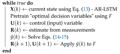
Notably, domain knowledge is encoded in controller model F for optimization and control vectors, providing the algorithm with understandability. Then, the constraints are implied for the hybrid MG system. The next step is to the conversion traditional MPC into S-MPC automatically. The last steps in the S-MPC are to solve the cost function and obtain "optimal decision variables", as shown in Algorithm 1. After that, the hybrid AR-LSTM method is initiated by configuring the controller model F. The current state is found using Equation (20) before training the "optimal control decisions". Finally, the control variable and are solved by utilizing updated reference and Equations (21) and (22).
| Algorithm 1:Switched Auto-regressive Neural Control (S-ANC) |
|
Identify:
Imply:
Switching logic: Conversion MPC into S-MPC
Solve: Objective function for S-MPC using Eq. (1)
Obtain: "Optimal decision variables"
Configure:
|
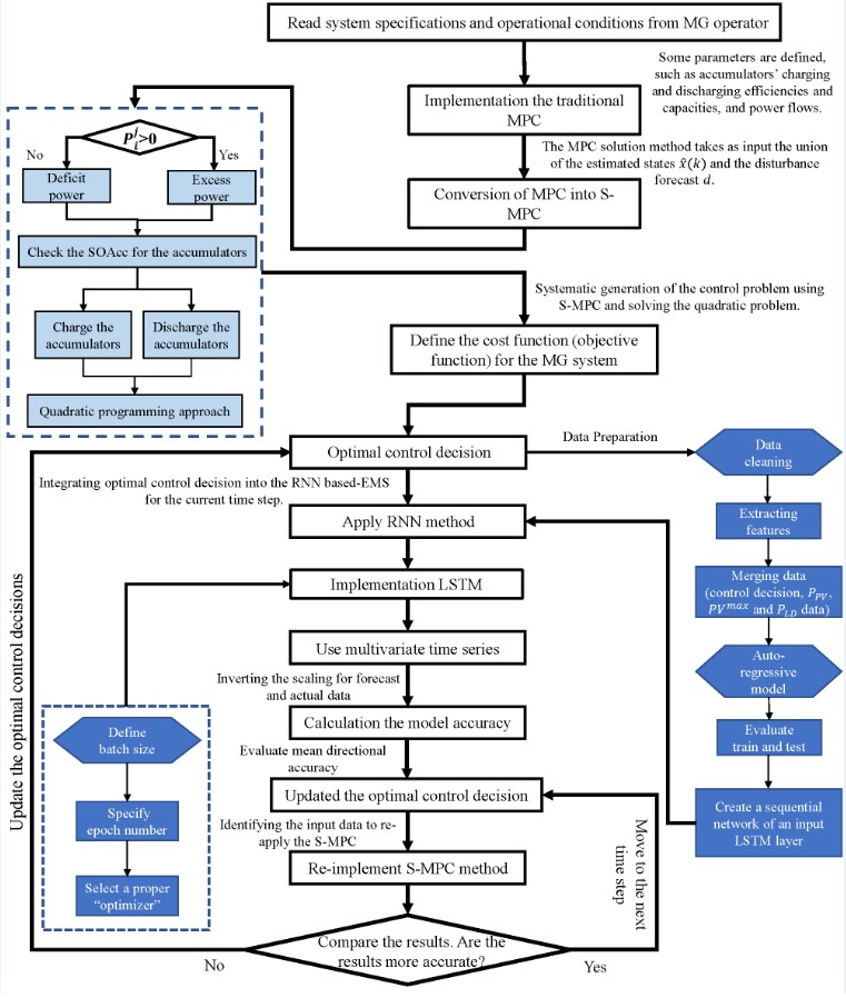
To begin, design a model of the MG system. The system reads some MG specifications, such as PV and load data, accumulator data, and maximum values of power flows among the components of hybrid MG. Following that, the MPC controller is implemented, which will state the optimization problem and solve it at each time step to obtain the optimal control inputs for the next time step. However, the MPC is converted into the S-MPC before it is applied. The optimization problem should consider the objectives and constraints in the paper’s methodology section. Implement an AR-LSTM model and train it on past data to increase the accuracy of the predictive model utilized by the S-MPC controller. Based on present and previous system conditions, the AR-LSTM should be able to anticipate future MG behaviour. The prediction should be input for the S-MPC controller’s optimization problem. Finally, as indicated in the methodology section of this paper, the S-MPC and AR-LSTM controllers in a closed-loop control system are combined. The proposed method can test the control strategy under various operating situations and evaluate its performance using the provided performance criteria (cost functions).
More specifically, to implement our proposed method into operation, initially, model the MG system and the S-MPC and AR-LSTM controllers and then combine these models into a closed-loop control system. Here are some detailed steps that need to be taken, as illustrated in Figure 5:
- Initiate the system specifications and operational conditions from the MG operator.
- Solve the systematic generation of the control problem employing the MPC with the QP.
- Using switching logic, convert the MPC into the S-MPC automatically.
- The optimal control decisions are obtained.
- The optimal control decisions are employed as input data for the AR method.
- The data preparation is initiated. The step has several parameters, such as data cleaning, extracting features, and merging the input data and PV constraints.
- The AR model is implemented to increase the accuracy of our proposed method.
- After that, the multivariate time series are employed.
- Then, the train and test data are selected and evaluated.
- To move the LSTM layer after the RNN, a sequential network of an input LSTM layer is produced.
- In this step (implementation of LSTM), several parameters are defined, including batch size, epoch number, and type of optimizer.
- Before moving the calculation to the model accuracy, the scaling for the forecast and actual data are inverted.
- The model accuracy is calculated using some methods, along with mean directional accuracy, method, and so on.
- Integrate the S-MPC and AR-LSTM controllers into a closed-loop control system by connecting the RNN output to the MPC controller’s input and the MPC controller’s output to the MG system’s input.
- Then, the optimal control decisions and references are updated. In other words, , , and are re-evaluated depending on the model accuracy.
- If this accuracy is unreasonable, the S-MPC is re-applied with the updated control decisions.
4. Results and Discussions
4.1. Case 1: The implementation of S-MPC
The non-optimal and optimal control (S-MPC) are compared for 96 hours (four days) in this case. In other words, in case 1, the emphasis is on the optimization of S-MPC and its effect on the power flows of the system (Figure 6) and SOC of the battery (Figure 6). Non-control methods employ simplistic control strategies or heuristic rules, disregarding the system’s dynamic nature. In addition, they do not have any constraints, so there are disadvantages associated with this strategy, such as poor SOC management, potential deviations from desired SOC levels, and inability to adapt to changing system conditions. As shown in Figure 6, the SOC of the battery goes below the critical value (20%) since the non-optimal method has no constraints. In contrast, the S-MPC method is an alternative to the non-optimal control method. S-MPC’s ability to dynamically select the appropriate model and control strategy based on the system’s current state is one of its key advantages. S-MPC optimizes control actions to achieve desired performance objectives, particularly in effectively managing the SOC of the battery.
The S-MPC controller has been designed to select the optimal model and control strategy based on the current operating mode and performance objectives. S-MPC enables enhanced power flow control and EM by effectively adapting to the changing dynamics of the hybrid MG, utilizing distinct models for each state. Case 1’s implementation of the S-MPC controller successfully optimizes the hybrid MG system’s power flows. It substantially reduces energy imports and increases energy exports, resulting in more efficient use of resources and enhanced energy flow management. The improved control strategy enables MG to operate closer to its optimal performance, enhancing its dependability and reducing operational costs. However, it is important to note that developing and implementing the S-MPC controller for the hybrid MG system presented obstacles due to the complex switching conditions and multiple operating modes. To guarantee the selection of the optimal model and control strategy, the switching logic had to be meticulously designed. The controller’s increased complexity required more computational resources than traditional MPC methods. The model’s computational time is almost 405 seconds.
4.2. Case 2: The implementation of the merged S-MPC and AR
Case 2 investigates the integration of the AR model with S-MPC. The AR models accurately predict future time steps by capturing the time series behaviour of the system. Various analyses, including variations, cross-validation (CV) iteration-Time Series Behaviour for training and validation, CV iteration-Training data on each CV iteration, and Predictions ordered by test prediction number, are used to evaluate the performance of the AR models.
Figure 7 that visualization is designed to provide insight into the behaviour of the lagged target feature over time. We can identify patterns, trends, or correlations within the lagged target data by examining the plot. Understanding the characteristics of the lagged target can aid in developing and optimizing an AR linear regression model that uses this characteristic for prediction. By displaying the lagging feature of the target, we can observe its values across multiple time steps. This lets us determine whether the lagged target exhibits specific patterns, trends, or variations over time.
As illustrated in Figure 7, variations in AR models illustrate their capacity to capture and model the system’s complex dynamics. By analyzing the CV iteration-Time Series Behaviour, the adaptability of the AR models to various patterns and tendencies in the training and validation data sets is assessed. This analysis sheds light on how models learn and generalize from available data, enabling accurate predictions for various time series problems.
Case 2’s successful integration of AR models with S-MPC illustrates the importance of incorporating time series behaviour and forecasting capabilities into the control system. Combining S-MPC and AR models permits enhanced adaptation to system dynamics and improves prediction accuracy, thereby enhancing the MG’s overall control performance.
4.3. Case 3: The implementation of the S-ANC
Case 3 examines the combination of S-MPC and AR-LSTM models. Integrating these advanced models aims to enhance the predictive capabilities of the control system. The S-ANC predicts the last month of the year using the first eleven months as training data. Using metrics such as train-test (Figure 8) and grid consumption prediction with AR regression and S-ANC (Figure 8), the performance of this merged approach is evaluated. This integration (S-MPC and AR-LSTM) increases the precision of forecasting and the precision of power flow optimization. The enhanced prediction capabilities of AR-LSTM models allow the control system to anticipate future energy requirements and adjust the operation of the MG accordingly. In Case 3, the S-MPC controller was improved by combining it with AR and RNN-LSTM models. The integration aimed to improve the precision of predictions and the overall performance of the control system. Two primary figures were generated for analysis: a comparison between the train and the test and a prediction of grid consumption using AR regression and S-ANC.
The train-test comparison diagram visually represents the AR-LSTM models’ capacity to generalize effectively to unobserved data. It compares the predicted grid consumption values during the testing phase with the actual values, indicating the AR-LSTM models’ ability to capture the hybrid MG’s complex patterns and dynamics (Figure 8). The diagram depicted the performance of the combined S-MPC, AR, and RNN-LSTM models on the training and testing data sets (Figure 8). According to our simulation, the model can generalize well to new data and the integration strategy’s effectiveness. Moreover, the prediction of grid consumption using AR regression and S-ANC illustrates the ability of the combined method to optimize power flows while accurately predicting future power demands. By leveraging the predictive capabilities of AR-LSTM models within the S-MPC framework, the control system can more precisely estimate grid consumption, allowing for more effective EM and enhancing the MG’s adaptability to load demands and renewable energy generation fluctuations. The grid consumption forecast graph (Figure 8) depicted projections generated by the AR and S-ANC models. It enabled a comparison of the two methods and highlighted the advantages of the S-ANC method, which employs the AR-LSTM model for accurate predictions while reducing computational time. The computational time of the model was reduced by nearly 214 seconds.
4.4. Calculation of model accuracy
To comprehensively evaluate the performance of the S-ANC prediction model, three unified evaluation indices, including R-squared Score, mean absolute error (MAE), and mean square error (MSE) [68,69], are selected in the paper. Each evaluation index has the following mathematical definition:
R-squared Score:
Mean Absolute Error:
Mean Squared Error:
where is the output vector using the S-MPC; represents the predicted value of the output vector by employing the S-ANC; represents the average value of output vector; n represents the total number of samples.
In this study, we assessed the performance of our predictive model using various metrics of accuracy. The R-squared error, which measures the proportion of the variance in the dependent variable that can be predicted from the independent variables, was 0.951. This suggests that our model can account for approximately 95.1% of the data’s variance, indicating a strong predictive ability. In addition, we determined that the MAE was 0.571. The MAE is the mean absolute difference between observed (from the MPC) and predicted values. A smaller MAE indicates that the predicted and observed values correspond more closely. In our case, the relatively low MAE indicates that our model’s predictions deviate from the true values, on average, by approximately 0.571%. Likewise, we determined the MSE to be 0.571. The MSE measures the average squared deviation between predicted and observed values. Similar to the MAE, a lower MSE indicates greater precision. The MSE value of our model indicates that the squared differences between the predicted and observed values are, on average, 0.571 units. Overall, the results show that our predictive model is effective. The relatively low MAE and MSE values of 0.571 indicate precise predictions with minimal deviations from the actual values.
5. Conclusions
Our findings show the efficacy and advantages of the S-ANC method for the intelligent control and management of hybrid MGs. The optimization of S-MPC improves energy management and power flow control, resulting in more efficient use of resources. The integration of AR and RNN-LSTM models improves the accuracy of predictions, allowing the control system to adapt to dynamic system conditions and optimize the operation of the MG. The successful implementation of S-ANC significantly affects the dependability, sustainability, and cost-effectiveness of hybrid MG systems. We can achieve efficient control and management of complex energy systems by leveraging the capabilities of advanced modelling techniques within the S-MPC framework. These findings support the incorporation of hybrid MGs into future energy systems and contribute to developing intelligent control strategies. By combining the AR-LSTM, the computational time of the model was reduced by approximately 47.2%. In addition, this study assessed the accuracy of our predictive model. The R-squared error, which quantifies the amount of variance in the dependent variable that can be predicted from the independent variables, was 0.951. Our model predicts 95.1% of the variance in the data, indicating a high level of predictive ability. The MAE and MSE values of 0.571 indicate precise forecasts with minimal deviations from actual values. The focus of future research and development should be validating larger-scale systems and incorporating additional advanced models. These developments will enhance the performance and applicability of the S-ANC methodology and contribute to the efficient operation and integration of hybrid MGs in future energy systems.
Author Contributions
Conceptualization, M.C., and Y.F.U.; methodology, M.C., A.A., and D.G.; software, M.C., and A.A.; validation, M.C., H.A., and A.A.; investigation, M.C.; writing—original draft preparation, M.C., and Y.F.U.; writing—review and editing, M.C., Y.F.U., H.A., A.A., K.A., and D.G.; visualization, M.C., Y.F.U. and H.A.; supervision, A.A., K.A., and D.G. All authors have read and agreed to the published version of the manuscript.
Institutional Review Board Statement
Not applicable.
Informed Consent Statement
Not applicable.
Data Availability Statement
Not applicable.
Conflicts of Interest
The authors declare no conflict of interest.
Abbreviations
The following abbreviations are used in this manuscript:
| ANN | Artificial Neural Network |
| AR | Auto-regressive |
| AR-LSTM | Auto-regressive Long Short-Term Memory |
| ARIMA | Auto-regressive Integrated Moving Average |
| ARMA | Auto-regressive Moving Average |
| BAT | Battery |
| BPTT | Back-Propagation Through Time |
| CNN | Convolutional Neural Network |
| CV | Cross-validation |
| DLC | Direct Load Control |
| EL | Electrolyzer |
| EM | Energy Management |
| ESS | Energy Storage System |
| FC | Fuel Cell |
| FT | Fuel Tank |
| GHI | Global Horizontal Irradiance |
| GR | Grid |
| GRU | Gated Recurrent Unit |
| IoT | Internet of Things |
| LSTM | Long Short-Term Memory |
| MAE | Mean Absolute Error |
| MG | Microgrid |
| MSE | Mean Squared Error |
| MILP | Mixed Integer Linear Programming |
| ML | Machine Learning |
| MPC | Model Predictive Control |
| NARX | Nonlinear Auto-regressive with exogenous input |
| NMG | Networked Microgrid |
| PAR | Peak-to-average Ratio |
| RNN | Recurrent Neural Network |
| RES | Renewable Energy Source |
| S-ANC | Switched Auto-regressive Neural Control |
| S-MPC | Switched Model Predictive Control |
| SVM | Support Vector Machine |
| QP | Quadratic Programming |
| WT | Water Tank |
| Charging efficiency of accumulator l | |
| Discharging efficiency of accumulator l | |
| F | controller model |
| H | constraint |
| J | objective function |
| Maximum values of power flows, 5 kW | |
| Photovoltaic | |
| or | Power flow from PV to grid |
| or | Power flow from PV to load |
| or | Power flow from grid to load |
| or | Power flow from PV to battery |
| or | Power flow from battery to load |
| or | Power flow from fuel cell to battery |
| or | Power flow from battery to electrolyzer |
| or | Hydrogen flow from electrolyzer to fuel tank |
| or | Hydrogen flow from fuel tank to fuel cell |
| or | Water flow from fuel cell to water tank |
| or | Water flow from water tank to electrolyzer |
| Flow of j from node a to node b | |
| Capacities of accumulator l, [kWh] | |
| Power of j from node a to node b | |
| Auto-regressive model coefficient | |
| Prediction horizon, 24h | |
| State of accumulator l | |
| Maximum value state of accumulator l | |
| Minimum value state of accumulator l | |
| error term or random noise at time k |
References
- Kumar, A.S.; Ahmad, Z. Model predictive control (MPC) and its current issues in chemical engineering. Chemical Engineering Communications 2012, 199, 472–511. [Google Scholar] [CrossRef]
- Garcia, C.E.; Prett, D.M.; Morari, M. Model predictive control: Theory and practice—A survey. Automatica 1989, 25, 335–348. [Google Scholar] [CrossRef]
- Pamulapati, T.; Cavus, M.; Odigwe, I.; Allahham, A.; Walker, S.; Giaouris, D. A Review of Microgrid Energy Management Strategies from the Energy Trilemma Perspective. Energies 2022, 16, 289. [Google Scholar] [CrossRef]
- Parisio, A.; Rikos, E.; Glielmo, L. A model predictive control approach to microgrid operation optimization. IEEE Transactions on Control Systems Technology 2014, 22, 1813–1827. [Google Scholar] [CrossRef]
- Ulutas, A.; Altas, I.H.; Onen, A.; Ustun, T.S. Neuro-fuzzy-based model predictive energy management for grid connected microgrids. Electronics 2020, 9, 900. [Google Scholar] [CrossRef]
- Silvente, J.; Kopanos, G.M.; Dua, V.; Papageorgiou, L.G. A rolling horizon approach for optimal management of microgrids under stochastic uncertainty. Chemical Engineering Research and Design 2018, 131, 293–317. [Google Scholar] [CrossRef]
- Parisio, A.; Rikos, E.; Glielmo, L. Stochastic model predictive control for economic/environmental operation management of microgrids: An experimental case study. Journal of Process Control 2016, 43, 24–37. [Google Scholar] [CrossRef]
- Garcia-Torres, F.; Bordons, C. Optimal economical schedule of hydrogen-based microgrids with hybrid storage using model predictive control. IEEE Transactions on Industrial Electronics 2015, 62, 5195–5207. [Google Scholar] [CrossRef]
- Jayachandran, M.; Ravi, G. Decentralized model predictive hierarchical control strategy for islanded AC microgrids. Electric Power Systems Research 2019, 170, 92–100. [Google Scholar] [CrossRef]
- Cavus, M.; Allahham, A.; Adhikari, K.; Zangiabadia, M.; Giaouris, D. Control of microgrids using an enhanced Model Predictive Controller. PEMD 2022. [Google Scholar] [CrossRef]
- Cavus, M.; Allahham, A.; Adhikari, K.; Zangiabadi, M.; Giaouris, D. Energy Management of Grid-Connected Microgrids using an Optimal Systems Approach. IEEE Access 2023. [Google Scholar] [CrossRef]
- Zhu, B.; Tazvinga, H.; Xia, X. Switched model predictive control for energy dispatching of a photovoltaic-diesel-battery hybrid power system. IEEE Transactions on Control Systems Technology 2014, 23, 1229–1236. [Google Scholar] [CrossRef]
- Maślak, G.; Orłowski, P. Microgrid operation optimization using hybrid system modeling and switched model predictive control. Energies 2022, 15, 833. [Google Scholar] [CrossRef]
- Moness, M.; Moustafa, A.M. Real-time switched model predictive control for a cyber-physical wind turbine emulator. IEEE Transactions on Industrial Informatics 2019, 16, 3807–3817. [Google Scholar] [CrossRef]
- Pervez, M.; Kamal, T.; Fernández-Ramírez, L.M. A novel switched model predictive control of wind turbines using artificial neural network-Markov chains prediction with load mitigation. Ain Shams Engineering Journal 2022, 13, 101577. [Google Scholar] [CrossRef]
- Magni, L.; Scattolini, R.; Tanelli, M. Switched model predictive control for performance enhancement. International Journal of Control 2008, 81, 1859–1869. [Google Scholar] [CrossRef]
- Aguilera, R.P.; Lezana, P.; Quevedo, D.E. Switched model predictive control for improved transient and steady-state performance. IEEE Transactions on Industrial Informatics 2015, 11, 968–977. [Google Scholar] [CrossRef]
- Kwadzogah, R.; Zhou, M.; Li, S. Model predictive control for HVAC systems—A review. 2013 IEEE International Conference on Automation Science and Engineering (CASE). IEEE, 2013, pp. 442–447.
- Forbes, M.G.; Patwardhan, R.S.; Hamadah, H.; Gopaluni, R.B. Model predictive control in industry: Challenges and opportunities. IFAC-PapersOnLine 2015, 48, 531–538. [Google Scholar] [CrossRef]
- Teimourzadeh, S.; Tor, O.B.; Cebeci, M.E.; Bara, A.; Oprea, S.V. A three-stage approach for resilience-constrained scheduling of networked microgrids. Journal of Modern Power Systems and Clean Energy 2019, 7, 705–715. [Google Scholar] [CrossRef]
- Oprea, S.V.; Bâra, A. Edge and fog computing using IoT for direct load optimization and control with flexibility services for citizen energy communities. Knowledge-Based Systems 2021, 228, 107293. [Google Scholar] [CrossRef]
- Bodong, S.; Wiseong, J.; Chengmeng, L.; Khakichi, A. Economic management and planning based on a probabilistic model in a multi-energy market in the presence of renewable energy sources with a demand-side management program. Energy 2023, p. 126549.
- Wynn, S.L.L.; Boonraksa, T.; Boonraksa, P.; Pinthurat, W.; Marungsri, B. Decentralized Energy Management System in Microgrid Considering Uncertainty and Demand Response. Electronics 2023, 12, 237. [Google Scholar] [CrossRef]
- Sansa, I.; Boussaada, Z.; Bellaaj, N.M. Solar Radiation Prediction Using a Novel Hybrid Model of ARMA and NARX. Energies 2021, 14, 6920. [Google Scholar] [CrossRef]
- Brahma, B.; Wadhvani, R. Solar irradiance forecasting based on deep learning methodologies and multi-site data. Symmetry 2020, 12, 1830. [Google Scholar] [CrossRef]
- Jeon, B.k.; Kim, E.J. Next-day prediction of hourly solar irradiance using local weather forecasts and LSTM trained with non-local data. Energies 2020, 13, 5258. [Google Scholar] [CrossRef]
- Husein, M.; Chung, I.Y. Day-ahead solar irradiance forecasting for microgrids using a long short-term memory recurrent neural network: A deep learning approach. Energies 2019, 12, 1856. [Google Scholar] [CrossRef]
- Zafar, R.; Vu, B.H.; Husein, M.; Chung, I.Y. Day-Ahead Solar Irradiance Forecasting Using Hybrid Recurrent Neural Network with Weather Classification for Power System Scheduling. Applied Sciences 2021, 11, 6738. [Google Scholar] [CrossRef]
- Qing, X.; Niu, Y. Hourly day-ahead solar irradiance prediction using weather forecasts by LSTM. Energy 2018, 148, 461–468. [Google Scholar] [CrossRef]
- Srivastava, S.; Lessmann, S. A comparative study of LSTM neural networks in forecasting day-ahead global horizontal irradiance with satellite data. Solar Energy 2018, 162, 232–247. [Google Scholar] [CrossRef]
- Wang, F.; Yu, Y.; Zhang, Z.; Li, J.; Zhen, Z.; Li, K. Wavelet decomposition and convolutional LSTM networks based improved deep learning model for solar irradiance forecasting. applied sciences 2018, 8, 1286. [Google Scholar] [CrossRef]
- Ghimire, S.; Deo, R.C.; Raj, N.; Mi, J. Deep solar radiation forecasting with convolutional neural network and long short-term memory network algorithms. Applied Energy 2019, 253, 113541. [Google Scholar] [CrossRef]
- Huang, J.; Korolkiewicz, M.; Agrawal, M.; Boland, J. Forecasting solar radiation on an hourly time scale using a Coupled AutoRegressive and Dynamical System (CARDS) model. Solar Energy 2013, 87, 136–149. [Google Scholar] [CrossRef]
- Jiang, Y.; Long, H.; Zhang, Z.; Song, Z. Day-ahead prediction of bihourly solar radiance with a Markov switch approach. IEEE Transactions on Sustainable Energy 2017, 8, 1536–1547. [Google Scholar] [CrossRef]
- Ekici, B.B. A least squares support vector machine model for prediction of the next day solar insolation for effective use of PV systems. Measurement 2014, 50, 255–262. [Google Scholar] [CrossRef]
- Yu, Y.; Cao, J.; Zhu, J. An LSTM short-term solar irradiance forecasting under complicated weather conditions. IEEE Access 2019, 7, 145651–145666. [Google Scholar] [CrossRef]
- Wojtkiewicz, J.; Hosseini, M.; Gottumukkala, R.; Chambers, T.L. Hour-ahead solar irradiance forecasting using multivariate gated recurrent units. Energies 2019, 12, 4055. [Google Scholar] [CrossRef]
- Zang, H.; Liu, L.; Sun, L.; Cheng, L.; Wei, Z.; Sun, G. Short-term global horizontal irradiance forecasting based on a hybrid CNN-LSTM model with spatiotemporal correlations. Renewable Energy 2020, 160, 26–41. [Google Scholar] [CrossRef]
- Gao, B.; Huang, X.; Shi, J.; Tai, Y.; Zhang, J. Hourly forecasting of solar irradiance based on CEEMDAN and multi-strategy CNN-LSTM neural networks. Renewable Energy 2020, 162, 1665–1683. [Google Scholar] [CrossRef]
- Connor, J.; Atlas, L. Recurrent neural networks and time series prediction. IJCNN-91-Seattle international joint conference on neural networks. IEEE, 1991, Vol. 1, pp. 301–306.
- Brownlee, J. Time series prediction with lstm recurrent neural networks in python with keras. Machine Learning Mastery 2016, 18. [Google Scholar]
- Moreno, J.J.M. Artificial neural networks applied to forecasting time series. Psicothema 2011, 23, 322–329. [Google Scholar]
- Shen, Z.; Zhang, Y.; Lu, J.; Xu, J.; Xiao, G. A novel time series forecasting model with deep learning. Neurocomputing 2020, 396, 302–313. [Google Scholar] [CrossRef]
- Bianchi, F.M.; Maiorino, E.; Kampffmeyer, M.C.; Rizzi, A.; Jenssen, R. Recurrent neural networks for short-term load forecasting: an overview and comparative analysis; Springer, 2017.
- Kumar, D.; Mathur, H.; Bhanot, S.; Bansal, R.C. Forecasting of solar and wind power using LSTM RNN for load frequency control in isolated microgrid. International Journal of Modelling and Simulation 2021, 41, 311–323. [Google Scholar] [CrossRef]
- Li, D.; Tan, Y.; Zhang, Y.; Miao, S.; He, S. Probabilistic forecasting method for mid-term hourly load time series based on an improved temporal fusion transformer model. International Journal of Electrical Power & Energy Systems 2023, 146, 108743. [Google Scholar] [CrossRef]
- DiPietro, R.; Hager, G.D. Deep learning: RNNs and LSTM. In Handbook of medical image computing and computer assisted intervention; Elsevier, 2020; pp. 503–519.
- Gupta, A.; Gurrala, G.; Sastry, P.S. Instability Prediction in Power Systems using Recurrent Neural Networks. IJCAI, 2017, pp. 1795–1801.
- Huo, Y.; Chen, Z.; Bu, J.; Yin, M. Learning assisted column generation for model predictive control based energy management in microgrids. Energy Reports 2023, 9, 88–97. [Google Scholar] [CrossRef]
- Cabrera-Tobar, A.; Massi Pavan, A.; Petrone, G.; Spagnuolo, G. A Review of the Optimization and Control Techniques in the Presence of Uncertainties for the Energy Management of Microgrids. Energies 2022, 15, 9114. [Google Scholar] [CrossRef]
- Zhou, Y. Advances of machine learning in multi-energy district communities–mechanisms, applications and perspectives. Energy AI 2022, 10, 100187. [Google Scholar] [CrossRef]
- Li, B.; Roche, R. Optimal scheduling of multiple multi-energy supply microgrids considering future prediction impacts based on model predictive control. Energy 2020, 197, 117180. [Google Scholar] [CrossRef]
- Nyong-Bassey, B.E.; Giaouris, D.; Patsios, C.; Papadopoulou, S.; Papadopoulos, A.I.; Walker, S.; Voutetakis, S.; Seferlis, P.; Gadoue, S. Reinforcement learning based adaptive power pinch analysis for energy management of stand-alone hybrid energy storage systems considering uncertainty. Energy 2020, 193, 116622. [Google Scholar] [CrossRef]
- Tang, W.; Zhang, Y.J. A model predictive control approach for low-complexity electric vehicle charging scheduling: Optimality and scalability. IEEE transactions on power systems 2016, 32, 1050–1063. [Google Scholar] [CrossRef]
- Karamanakos, P.; Geyer, T.; Kennel, R. A computationally efficient model predictive control strategy for linear systems with integer inputs. IEEE Transactions on Control Systems Technology 2015, 24, 1463–1471. [Google Scholar] [CrossRef]
- Zhang, L.; Zhuang, S.; Braatz, R.D. Switched model predictive control of switched linear systems: Feasibility, stability and robustness. Automatica 2016, 67, 8–21. [Google Scholar] [CrossRef]
- Ayumi, V.; Rere, L.R.; Fanany, M.I.; Arymurthy, A.M. Optimization of convolutional neural network using microcanonical annealing algorithm. 2016 International Conference on Advanced Computer Science and Information Systems (ICACSIS). IEEE, 2016, pp. 506–511.
- Liu, C.T.; Wu, Y.H.; Lin, Y.S.; Chien, S.Y. Computation-performance optimization of convolutional neural networks with redundant kernel removal. 2018 IEEE international symposium on circuits and systems (ISCAS). IEEE, 2018, pp. 1–5.
- Huang, R.; Wei, C.; Wang, B.; Yang, J.; Xu, X.; Wu, S.; Huang, S. Well performance prediction based on Long Short-Term Memory (LSTM) neural network. Journal of Petroleum Science and Engineering 2022, 208, 109686. [Google Scholar] [CrossRef]
- Zhang, Y.; Hao, X.; Liu, Y. Simplifying long short-term memory for fast training and time series prediction. Journal of Physics: Conference Series. IOP Publishing, 2019, Vol. 1213, p. 042039.
- Schmidt, R.M. Recurrent neural networks (rnns): A gentle introduction and overview. arXiv preprint arXiv:1912.05911 2019. arXiv:1912.05911 2019.
- Amidi, A.; Amidi, S. Vip cheatsheet: Recurrent neural networks, 2018.
- Ruder, S. An overview of gradient descent optimization algorithms. arXiv preprint arXiv:1609.04747 2016. arXiv:1609.04747 2016.
- Görges, D. Relations between model predictive control and reinforcement learning. IFAC-PapersOnLine 2017, 50, 4920–4928. [Google Scholar] [CrossRef]
- Ying, X. An overview of overfitting and its solutions. Journal of physics: Conference series. IOP Publishing, 2019, Vol. 1168, p. 022022.
- Giaouris, D.; Papadopoulos, A.I.; Patsios, C.; Walker, S.; Ziogou, C.; Taylor, P.; Voutetakis, S.; Papadopoulou, S.; Seferlis, P. A systems approach for management of microgrids considering multiple energy carriers, stochastic loads, forecasting and demand side response. Applied energy 2018, 226, 546–559. [Google Scholar] [CrossRef]
- Cavus, M.; Allahham, A.; Adhikari, K.; Giaouris, D. A Hybrid Method Based on Logic Control and Model Predictive Control for Synthesizing Controller for Flexible Hybrid Microgrid with Plug-and-Play Capabilities. Available at SSRN 447 3008.
- Chicco, D.; Warrens, M.J.; Jurman, G. The coefficient of determination R-squared is more informative than SMAPE, MAE, MAPE, MSE and RMSE in regression analysis evaluation. PeerJ Computer Science 2021, 7, e623. [Google Scholar] [CrossRef]
- Kong, X.; Du, X.; Xu, Z.; Xue, G. Predicting solar radiation for space heating with thermal storage system based on temporal convolutional network-attention model. Applied Thermal Engineering 2023, 219, 119574. [Google Scholar] [CrossRef]
Figure 1.
Block diagram of (a) S-MPC and (b) AR-LSTM.
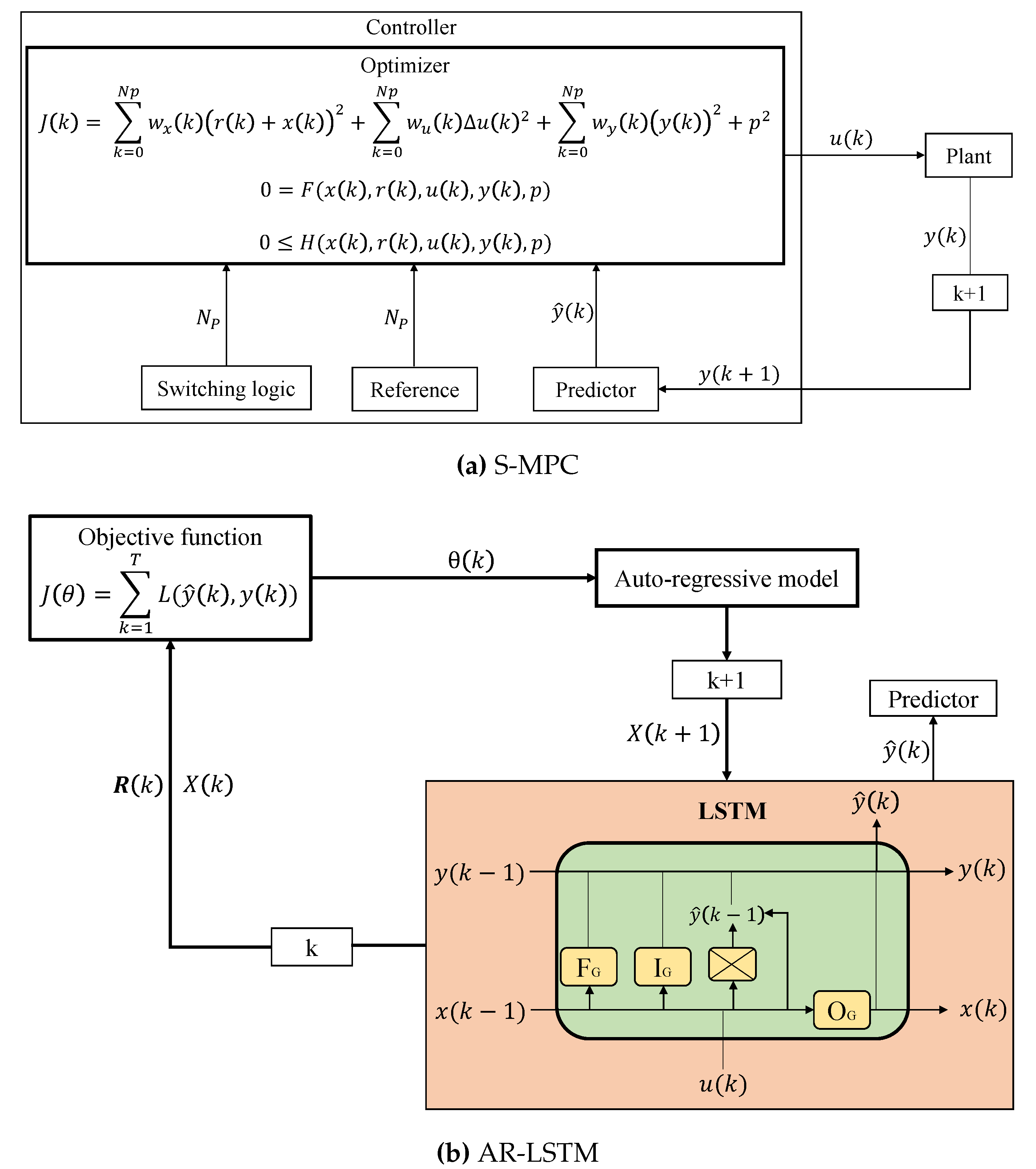
Figure 2.
Structure of the RNN.
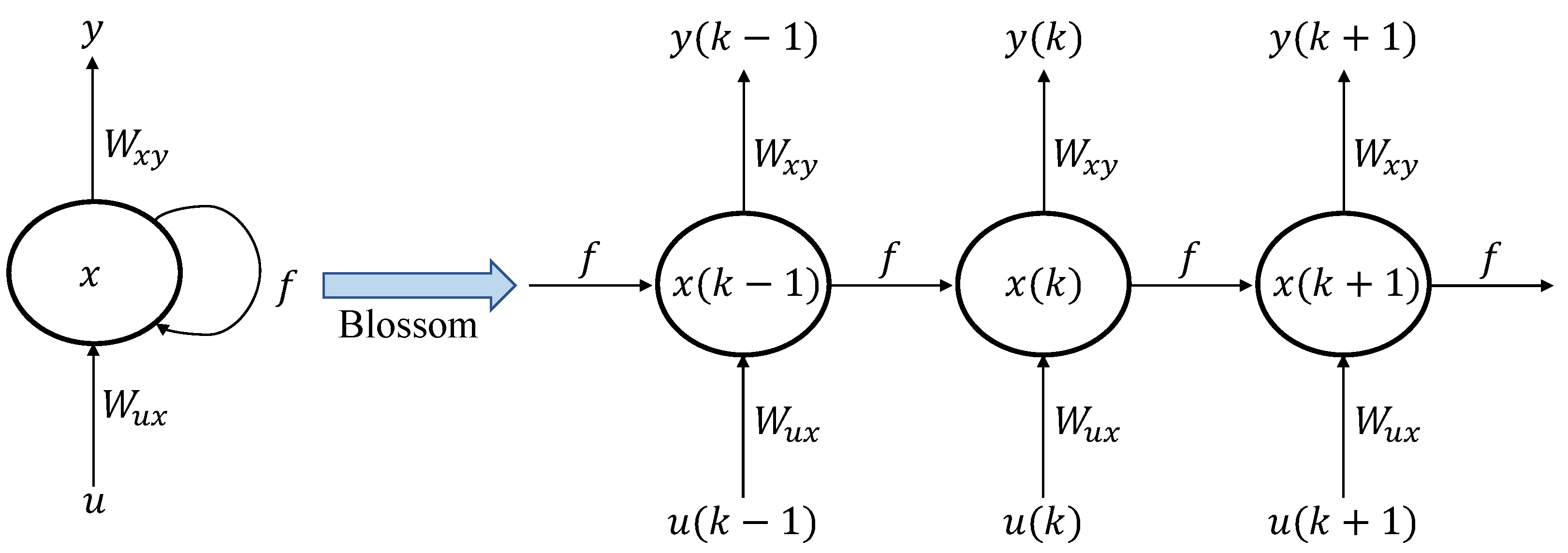
Figure 3.
Hybrid MG Structure.
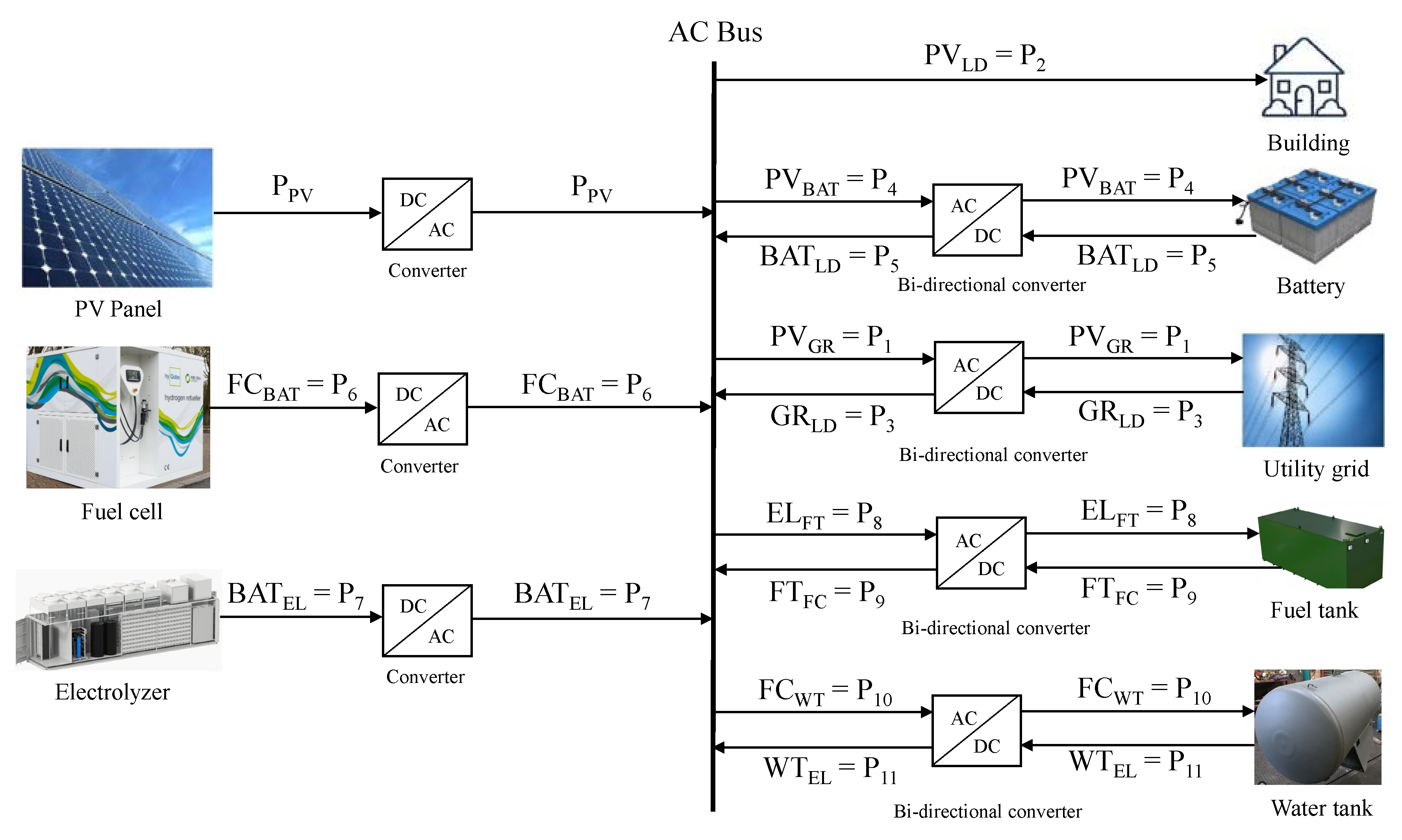
Figure 4.
Block diagram showing the introduction of S-ANC.
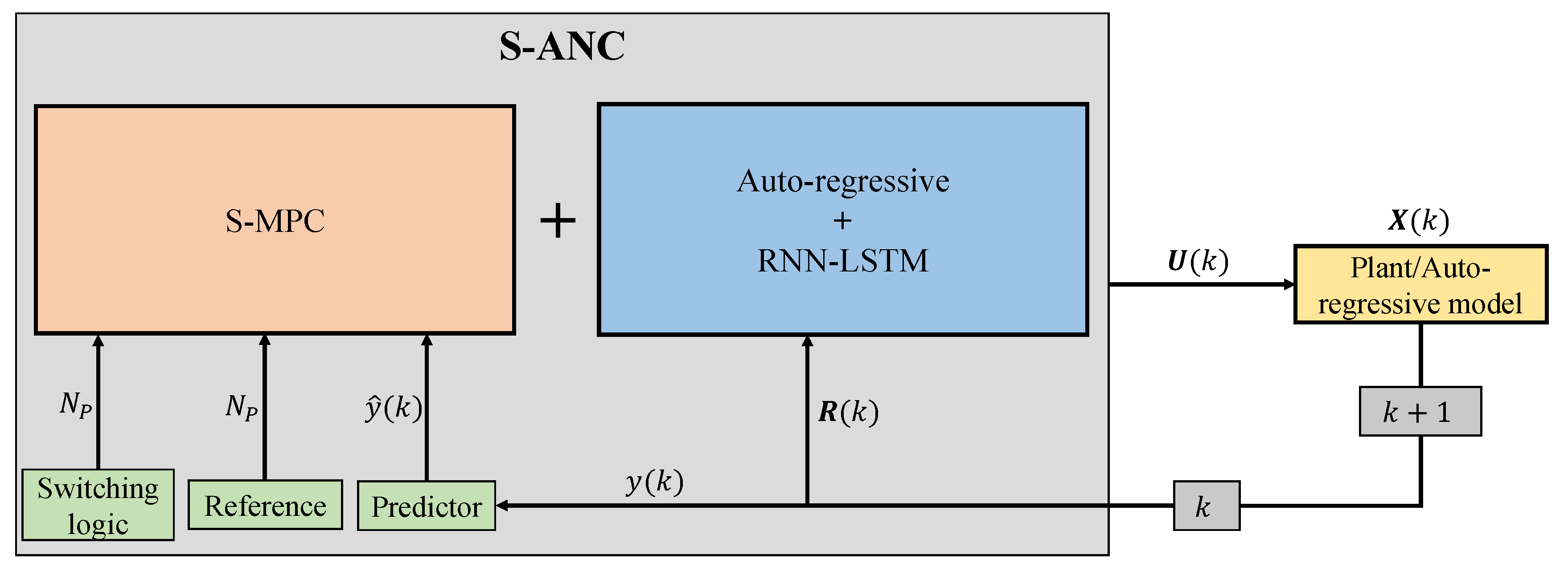
Figure 5.
Flow chart of the proposed method.
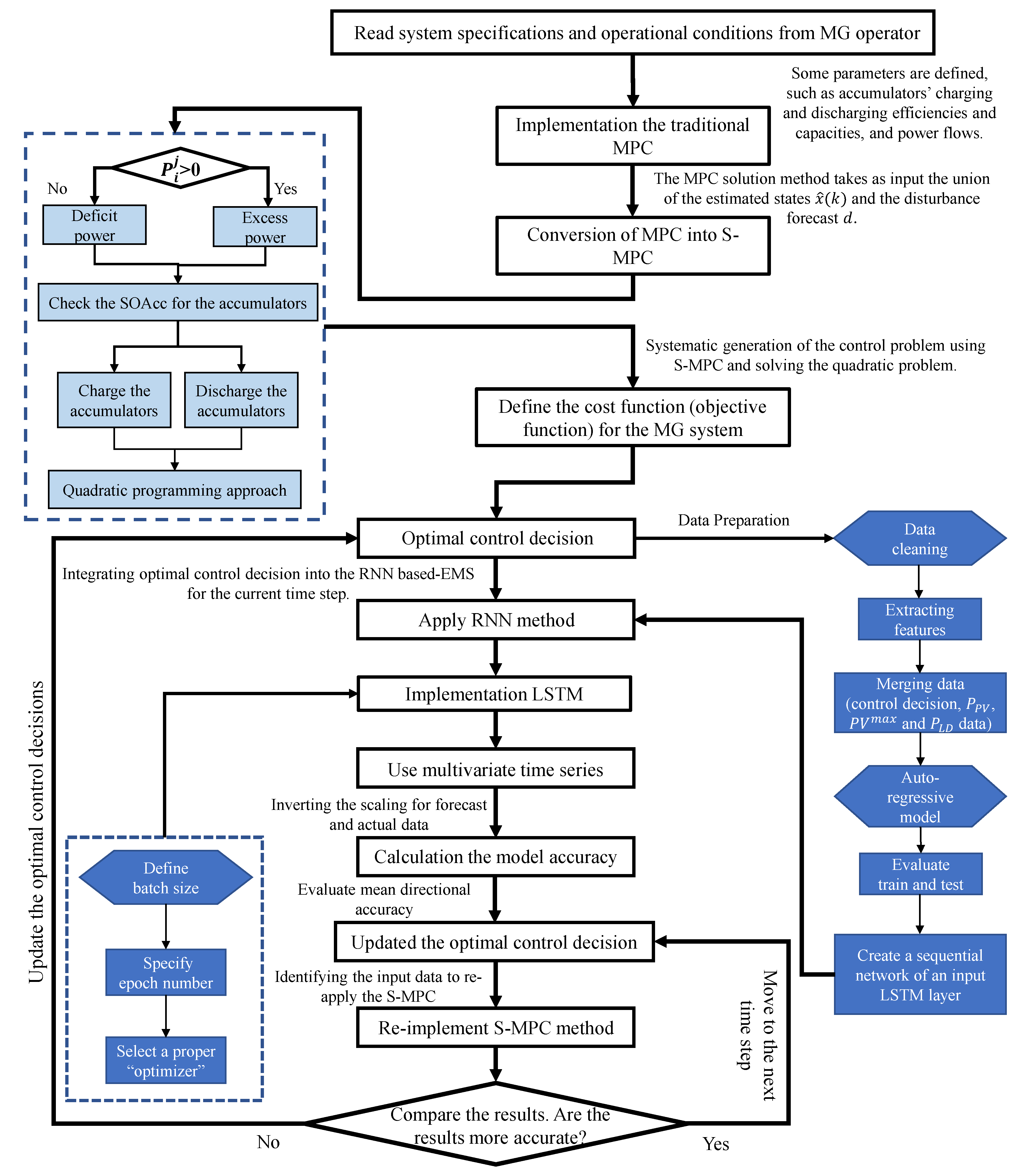
Figure 6.
The comparison of (a) power flows and (b) SOC of the battery using optimal method (S-MPC) and non-optimal method.
Figure 6.
The comparison of (a) power flows and (b) SOC of the battery using optimal method (S-MPC) and non-optimal method.
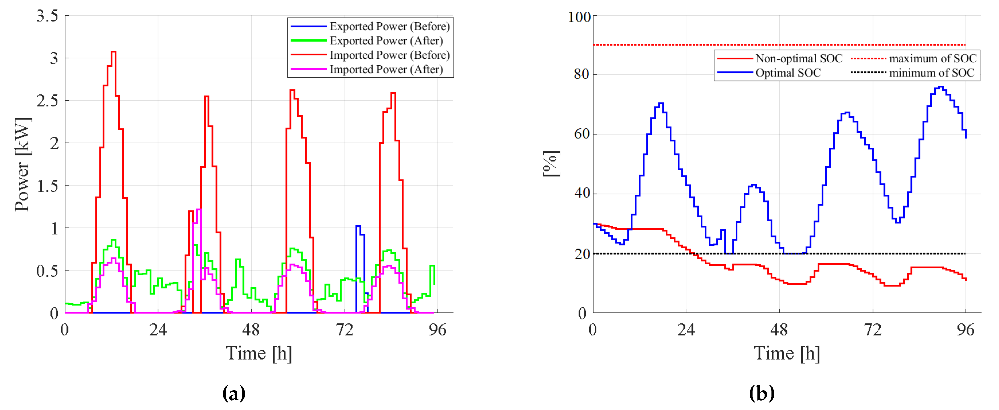
Figure 7.
The visualization of (a) the behaviour of the lagged target feature over time, (b) the adaptability of the AR models to various patterns and tendencies
Figure 7.
The visualization of (a) the behaviour of the lagged target feature over time, (b) the adaptability of the AR models to various patterns and tendencies
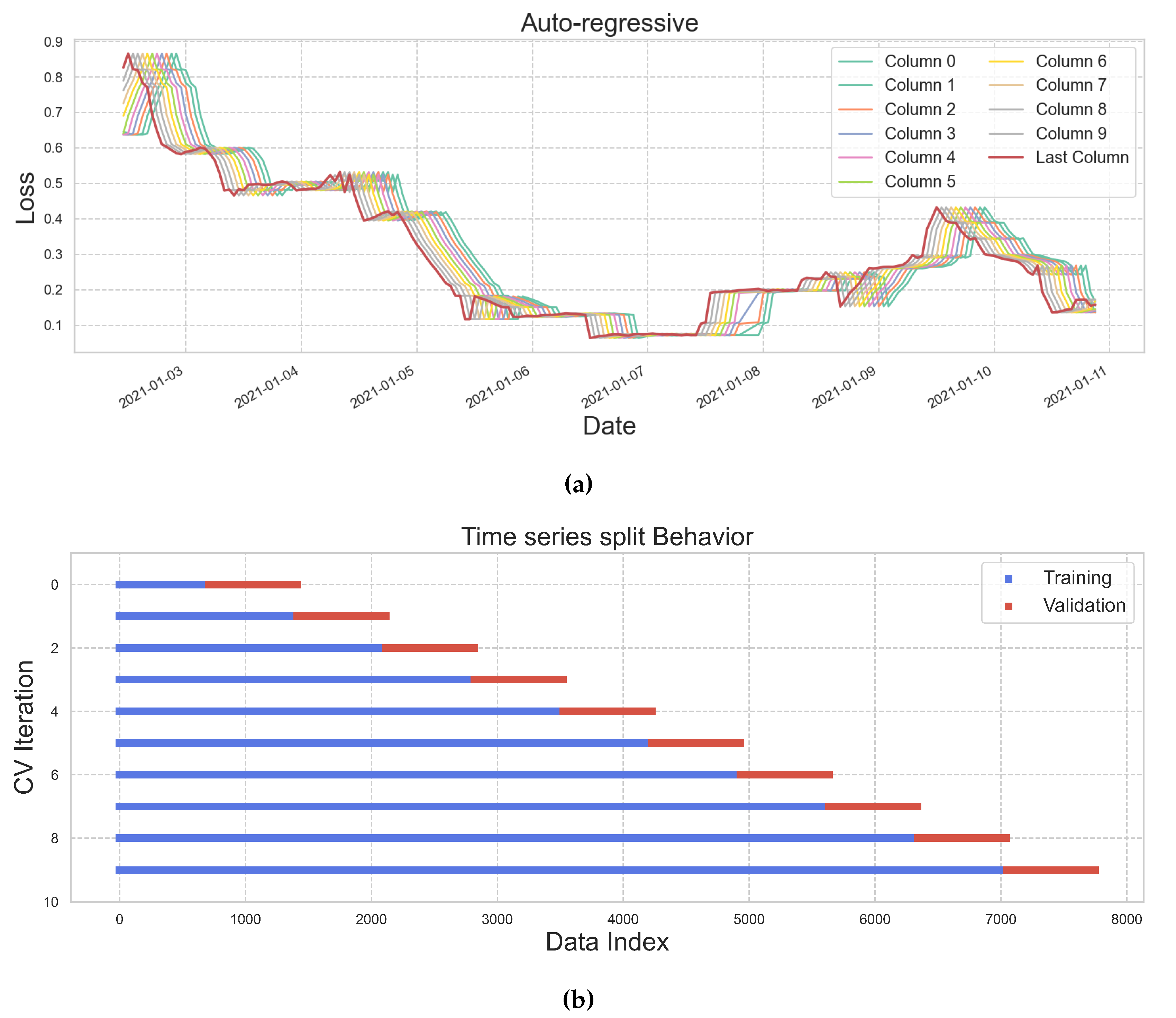
Figure 8.
The illustration of (a) train-test data and (b) prediction of grid consumption using AR regression and S-ANC.
Figure 8.
The illustration of (a) train-test data and (b) prediction of grid consumption using AR regression and S-ANC.
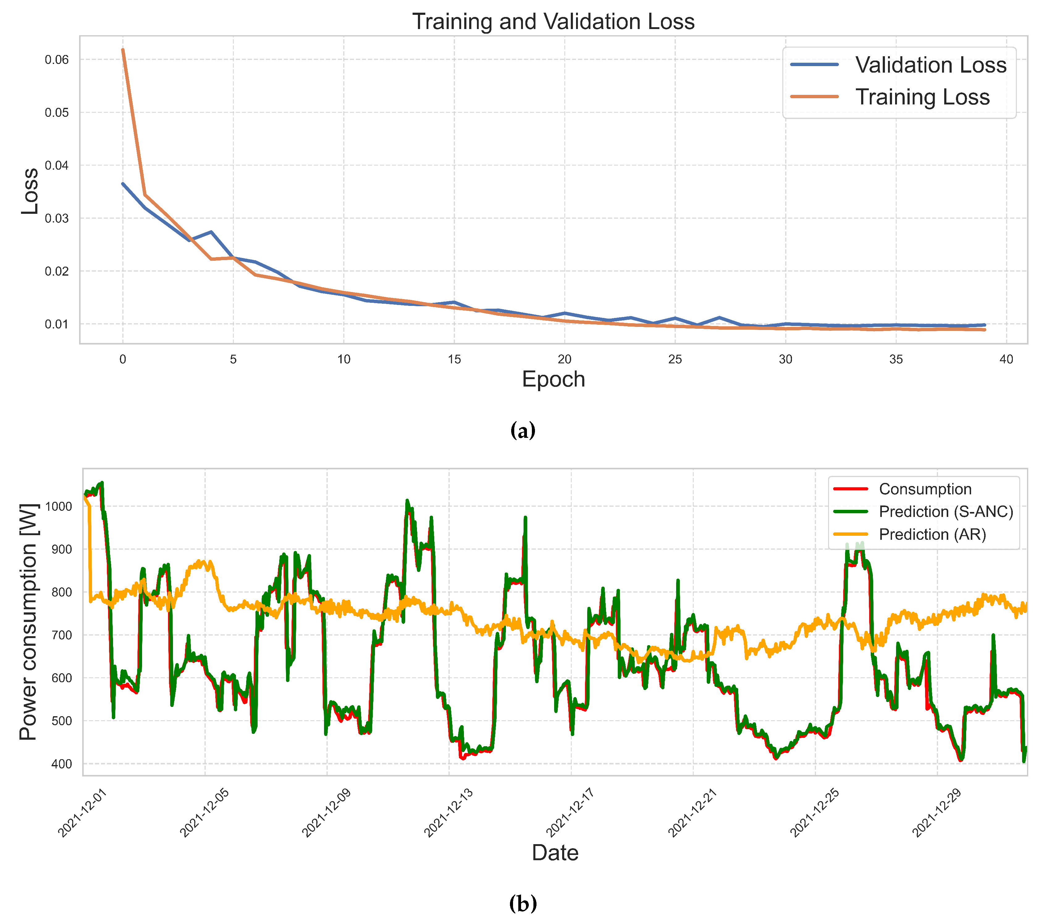

Table 1.
Comparison of Control Methods.
| Control Method | Optimality | Computational Time [s] | Multiple Models | Adaptability | Constraints |
|---|---|---|---|---|---|
| MPC [54,55] | ✓ | [High] | × | Good | ✓ |
| S-MPC [10,11,15,56] | ✓ | [Moderate] | ✓ | Outstanding | ✓ |
| DLC [21] | ✓ | [Moderate] | × | Good | ✓ |
| AR [24] | × | [Moderate] | × | Poor | × |
| CNN [57,58] | × | [Low] | × | Poor | × |
| RNN-LSTM [59,60] | ✓ | [Low] | × | Poor | × |
| S-ANC | ✓ | [Low] | ✓ | Outstanding | ✓ |
Disclaimer/Publisher’s Note: The statements, opinions and data contained in all publications are solely those of the individual author(s) and contributor(s) and not of MDPI and/or the editor(s). MDPI and/or the editor(s) disclaim responsibility for any injury to people or property resulting from any ideas, methods, instructions or products referred to in the content. |
© 2023 by the authors. Licensee MDPI, Basel, Switzerland. This article is an open access article distributed under the terms and conditions of the Creative Commons Attribution (CC BY) license (http://creativecommons.org/licenses/by/4.0/).
Copyright: This open access article is published under a Creative Commons CC BY 4.0 license, which permit the free download, distribution, and reuse, provided that the author and preprint are cited in any reuse.


