1. Introduction
Recent years, hyperspectral remote sensing technology has made significant strides which uses spectroscopy imagery technology to synchronously gather enormous spectral and spatial information of the observing targets at pixel level[
1], thus enabling to conduct accurate classification for the observation targets[
2,
3,
4]. Numerous fields including ecological research[
5], precision agriculture[
6], mineral exploration[
7], and medicine[
8], are covered by the categorization tasks of HSI considering the advantage of a wealth of information contained in it. Unlike some other image classification missions, HSI classification is an operation which carried out at pixel-wise, assigning each of the pixels in the imagery into a specific category[
9].
In the early stage of the study on the HSI classification, the spectral information played the leading role. Most methods focus on exploring the discrepancy of original spectral signatures in HSI to distinguish the pixels into different categories, including k-nearest neighbor(KNN)[
10], support vector machines(SVM)[
11], logistic regression[
12], and so on. However, the original spectral features in HSI always obey a complex high-dimensional nonlinear distribution where traditional machine learning based methods can not handle it well. In light of this, direct exploration of the original spectral vectors leads to a large computing cost as well as decreased classification performance. Thus, several methods for dimension reduction and spectral information extraction have also been developed, such as PCA[
13,
14], ICA[
15], and LDA[
16]. Despite the fact that several standard spectral feature extraction methods may extract useful spectral features, the basic linear processing present in these linear models makes it sitll difficult to manage the complicated spectrum properties of HSIs.
With the advancement of deep learning, recent research in the domain of hyperspectral image classification has predominantly relied on deep learning based methodologies. Thanks to their robust representational capabilities, these approaches have led to a notable enhancement in classification performance. For insistence, Ahmad et al.[
17] and Mughees et al[
18]. gathered the feature sets by using a autoencoder(AE) based method to extract HSI features. Zhong et al.[
19] proposed a semi-supervised deep belief networks(DBN), this method through regularizing pretraining and fine-tuning procedures by a diversity promoting prior over latent factors,thereby improving model classification performance. Nevertheless, owing to inherent challenges in hyperspectral imagery, such as spectral drift, spectral variability within identical materials, and material variability within identical spectra, methods that directly incorporate spectral information continue to exhibit a significant number of classification errors. To address this issue, convolutional neural networks (CNNs) have been introduced into the research on hyperspectral image classification, where a pixel and its neighbors in a hyperspectral image are taken as inputs of the CNN, and the final CNN output is the predicted class labels[
20,
21,
22,
23]. The architectural design of such networks not only incorporates translational invariance but also effectively introduces an inductive bias, implying that pixels within the same patch are likely to belong to the same land cover class. Furthermore, to harness spectral information more effectively, 3D convolutions have been incorporated into this research. For examples, Xu et al[
24]. designed a multiple spectral resolution 3D convolutional neural network (MSR-3DCNN) where combined the 3D convolution layer and residual connection to better adapt to the 3D cubic form of hyperspectral data and make efficient use of spectral information in different bands. Li et al[
25]. combined depthwise separable convolution and 3DCNN, this work successfully accelerated the training speed and achieved good classification performance.
While convolutional network structures have demonstrated strong performance in this domain, certain limitations persist, constraining the network’s overall performance. The additional inductive bias introduced by convolutional operations may not be applicable to pixels located at the boundaries of land cover regions. For instance, within the same patch, there may exist a variety of pixels belonging to distinct land cover classes. Furthermore, due to the sensitivity of convolutions to geometric textures in images, boundaries between land cover regions are also prone to extraction, introducing noise during classification[
26]. In the context of convolutional mechanisms for hyperspectral image classification, a limitation arises due to the convolutional operations being performed on the neighborhood of target pixels. Typically, when the neighborhood size is fixed, the structure of the convolutional network becomes rigid, resulting in a singular input scale and limited generalization performance[
27]. Altering the neighborhood size necessitates a corresponding modification in the convolutional network structure, rendering previously trained model parameters unusable and leading to inefficient data utilization.
To surmount these inherent deficiencies of convolutional neural networks, certain research endeavors opt to employ Transformer modules as foundational structures in designing classification models[
27,
28,
29,
30,
31,
32,
33,
34]. Models of this nature have demonstrated the capacity to surmount the inherent limitation of fixed input dimensions in convolutional networks, resulting in superior performance in high-dimensional spectral image classification tasks compared to convolutional neural networks. However, their generalization capabilities remain unverified, and due to the absence of inductive biases in Transformer networks, they often necessitate a larger volume of data for effective fitting to achieve optimal performance[
35]. In the realm of natural language processing tasks, pre-trained large-scale models have exhibited remarkable performance, showcasing robust generalization and transfer capabilities, even when exposed to a limited amount of downstream task-specific annotations[
36,
37]. Prominent examples include BERT[
38] and the GPT series[
39,
40,
41]. Building upon the foundation laid by Vision Transformers(ViT)[
42], researchers have devised pre-training models tailored for the visual domain, such as Google’s BEiT[
43] and the MAE model developed by the team led by Kaiming He et al[
44]. These methods employ self-supervised learning techniques for model pre-training and have consistently achieved state-of-the-art performance in downstream tasks. Scholars, drawing inspiration from this concept, have devised pre-trained models tailored for hyperspectral imagery. These models have demonstrated commendable performance in classification tasks, exemplified by Masked Autoencoding Spectral–Spatial Transformer(MAEST) designed by Ibanez et al.[
45], Spectral–Spatial Masked Transformer(SS-MTr) proposed by Huang et al.[
46] and Masked spatial-spectral model(Masked SST) raised by Scheibenreif et al.[
47] However, it is noteworthy that these models have primarily leveraged a limited subset of hyperspectral data available in the public domain, such as Indian Pines, PaviaU and Salinas Dataset. Moreover, when employing these models on different datasets, apart from fine-tuning on the new data, retraining on the new dataset is often necessary. These methodologies have not fully harnessed the extensive reservoir of unlabeled hyperspectral data that is accessible and have maintained certain constraints on network inputs.
Inspired by these insights, this study introduces a pre-trained model specifically designed for hyperspectral images, employing the Transformer architecture as its foundational framework. This model boasts the ability to process patches of arbitrary dimensions and exhibits remarkable generalization capabilities across varying spectral resolutions within hyperspectral imagery. Within this model, we implement a self-supervised training strategy inspired by the methodology employed in MAE. This involves the random masking of individual pixels within each patch, followed by their passage through an encoder-decoder network structure, ultimately facilitating the reconstruction of the original, unmasked patch. During this process, each pixel, serving as a carrier of spectral information, can be analogously likened to words in the context of natural language processing. Meanwhile, the spatial relationships between these pixels are reminiscent of contextual information in NLP. Consequently, the network inherently acquires an understanding of spatial spectral information within hyperspectral images as it undertakes the patch reconstruction task. To accommodate variable input sizes, this study introduces adaptable conditional positional embedding.[
48] In response to the inherent absence of inductive biases within Transformer architectures, we propose a novel approach. This entails the incorporation of an
at the input side of the model’s encoder, initialized with random values. Leveraging a metric learning paradigm[
49], we aim to align the output vector of this
, post-decoding, as closely as possible with the embedding vector of the target pixel within a designated projection space. This strategic augmentation serves to direct the model’s attention towards the specific target pixel. In the context of downstream tasks, instead of global average pooling(GAP)[
50], we introduce a mechanism to adaptively combine the tokens generated by the encoder to fully exploit the knowledge acquired by the network. The resulting composite output is subsequently utilized as the ultimate classification vector, which is then fed into the classifier for supervised training.
To facilitate the training of our model, we undertook a comprehensive data curation process, sourcing a diverse collection of hyperspectral images from the Gaofen-5 satellite. This dataset encompassed a broad spectrum of environmental scenarios, ranging from desert, forest, township, forest village, snowfield, village, city and metropolis. Subsequently, we meticulously divided these unlabeled images into non-overlapping patches, categorized into four distinct size parameters. When transferring pre-trained model parameters to a new dataset, the process primarily involves the replacement of the network’s input layer to accommodate varying spectral resolutions. Subsequently, supervised fine-tuning can be conducted with a limited number of samples. In the same circumstances, compared to similar, our technique delivered state-of-the-art performance.
In summary, the primary contributions of this paper are as follows:
We have devised a pre-trained model capable of effectively harnessing a substantial volume of unlabeled hyperspectral imagery. This model significantly enhances data utilization efficiency and augments downstream task performance, particularly in scenarios characterized by limited sample availability.
We have introduced a model instructor, denoted as the , a randomly initialized vector that effectively directs the model’s focus toward areas of human interest through metric learning.
Our proposed model exhibits robust generalization capabilities while maintaining simplicity and ease of implementation.
We have curated a comprehensive hyperspectral imaging (HSI) pre-training dataset, encompassing a multitude of environmental scenarios and varying input sizes.
2. Methodology
2.1. Overview of IMAE
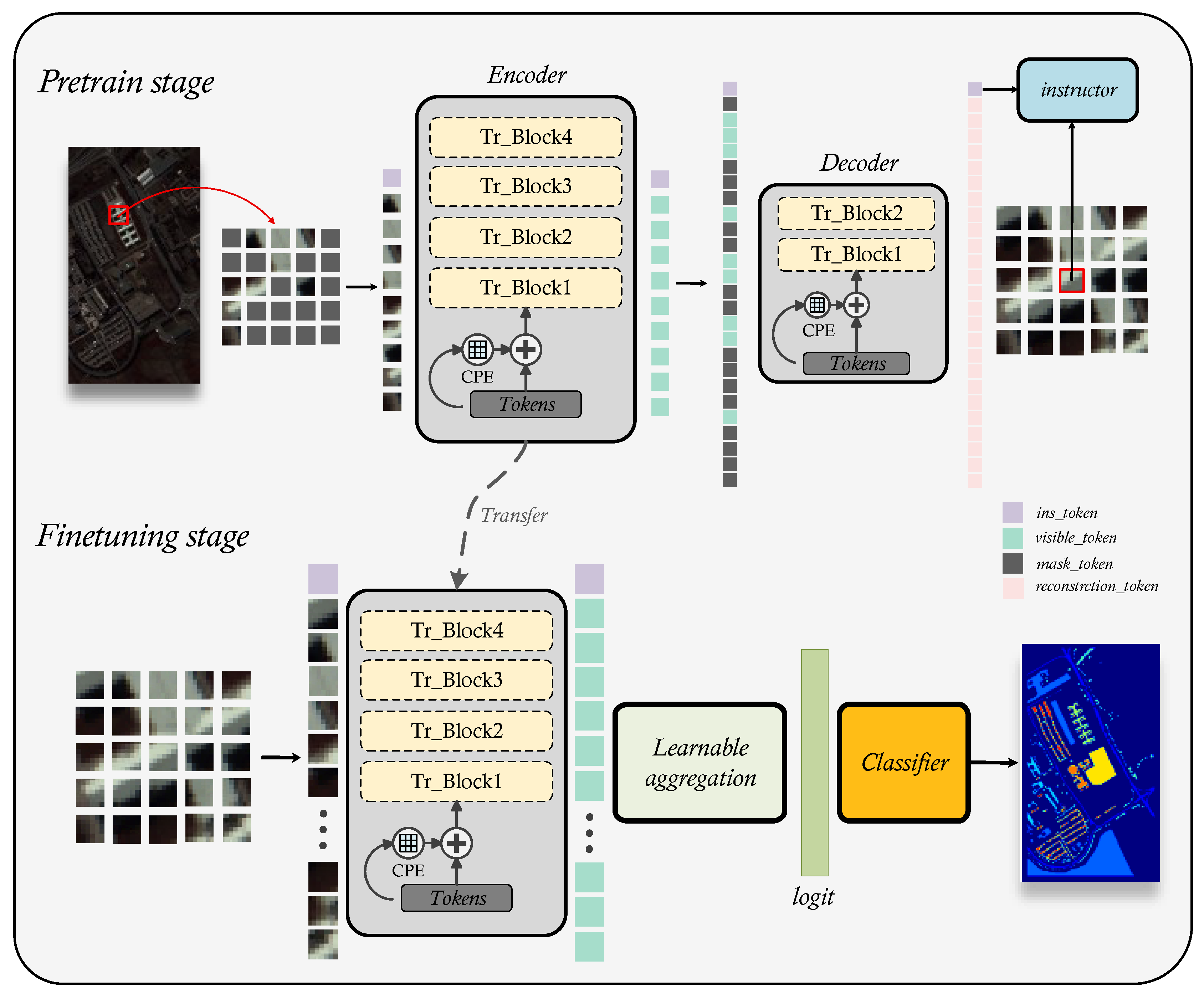
Inspired by recent self-supervised models for computer vision, we design a transformer-based HSI classification pre-training model that automatically extracts general features of hyperspectral images through two self-supervised proxy tasks. After pre-training is completed, the model can be easily transferred to any hyperspectral remote sensing data. To keep employing the common sense the model has learnt, regardless of how the HSI’s spectral resolution changes, we just need to alter the model’s first input layer parameters. In this section, we first introduce the overview of IMAE. Afterwards, we will present the primary components of the network in detail, including spectral embedding, instructor masked autoencoder and learnable aggregation.
In this work, we use ViT as the backbone and construct a masked autoencoder to extract general spatial spectral features of HSI. Normally, ViT needs to execute linear embedding on the patch before encoding the extracted image information into a token, the input of model is the whole image. In contrast to RGB images, HSI includes abundant spectral information that could indicate material attributes. Therefore, we embed each spectral signal in the patch into token, this means we use the patch as the model input. In this method, we combine 3D convolution and 2D convolution and use a 1*1 convolution kernel to perform linear embedding of spectral information to achieve spectral feature extraction while maintaining the correlation between different band of spectra. In transformer, position embedding is a very important component for the extraction of spatial information. Usually, a predefined position embedding method is used to generate the position tokens. This method has a fixed length and is independent of the input tokens and can’t fully utilize neighborhood information. Therefore, we use conditional position embedding to generate the position tokens. That strategy is learnable which considers both the neighborhood and semantic information of the token and it can be easily generalized to token sequences of various lengths. For the analysis of HSIs, humans mainly concentrate on the central pixel of the patch merely the transformer-based model performs global feature extraction on the patch, which namely local attention distraction. Therefore, we teach the model, by integrating an instructor token named
, how to infer the information embedded in the central pixel from the global information of the patches, thus model naturally learns this domain prior. Moreover, this method can help model focus on the in interested region regardless of the size of the input. In downstream tasks, in order to fully utilize the information contained in tokens, instead of GAP, we design a learnable aggregation strategy for the output tokens of encoder. The overall architecture of IMAE is illustrated in
Figure 1.
2.2. Spatial-spectral embedding
The spatial-spectral embedding is mainly composed of two basic components which are spectral embedding and position embedding. We first present our spectral embedding procedure in this section, followed by the positional encoding strategy.
The standard vision transformer divides the entire image into non-overlapping patches and then encodes these patches into a token sequence. However, the patch-level feature extraction is not suitable for the analysis of HSIs. Given it typically conduct pixel-level analysis when analyzing HSIs, thus the spectral embedding require more fine-grained features. Specifically, we adjust the input of the model to patch, then preform embedding on the spectral signal. We give up the dimensionality reduction approach of some independent components, like PCA, ICA, etc, to prevent breaking the correlation between different spectral bands. In our spectral embedding strategy,
convolution kernels in combination with 2D and 3D convolution are used to perform feature embedding on the spectral dimension in order to obtain the maximum spectral information possible. Given a traning sample
,
, where
h and
w represent the height and width of the input patch,
b represents the number of bands. In 2D convolution operation, the
lth convolution kernel
,
, the feature map of
is
. For illustration, consider the input layer, we calculate
according to the equation
1.
In 3D convolution operation, the
lth convolution kernel
,
, the feature map of
is
. As a demonstration, suppose the input data
, we calculate
according to the equation
2.
Where
s represents the stride of the 3D convolution kernel on third dimension of the input, the third dimension
c of
can be computed as equation
3.
We construct the spectral embedding(
) module using two 2D convolution layers and a 3D convolution layer, and its expression is as equation
4.
In addition, position embedding plays a crucial role in the transformer-based model. Through the self-attention mechanism, the transformer-based model can learn the relationships between tokens and pay attention to essential facts, but it is unable to learn the precise positions of each token, thus necessitating the input of extra token position information to the model. Position embedding is an approach for re-representing each token in the sequence with the token’s position information so that the input tokens carrier the position information and the model can learn the features of the positions. The common position embedding methods are predefined, the length of position token sequence is fixed even if the position tokens are learnable, which will make the model unable to handle sequences exceeding the predefined length. The sequence length growth in a HSI patch is a square term of its size, so using the length fixed embedding method will prevent the model from generalizing to larger patch inputs. Furthermore, the pre-defined methods just add a particular encoding to each token in accordance with the sequence, disregarding the relationship between the pixels in the patch and the neighborhood in which they are located.
Conditional position embedding is a flexible, parameter-free approach which can solve this defect. It hinges on the the input token and its neighborhood to dynamically produce the position embedding token associated with the input token. Moreover, CPE is translation-invariant which allows it to efficiently leverage the local homogeneity of natural images. CPE can be easily implemented by 2D convolution layer and same padding layer.
Figure 2 illustrates the structure of CPE. After spectral embedding(
) and position embedding(
), the input of the transformer is:
where
,
c reperesents the embedding dimension.
2.3. Instructor Masked AutoEncoder for HSI spectral-spatial feature extraction
In this section, we focus on how to extract general features in hyperspectral images through IMAE. Concretely, we perform self-supervised training for IMAE through constructing two proxy tasks, which are constructing a pixel-level masked autoencoder to reconstruct the random masked input as well as designing a instructor token to direct the model to concentrate on the region we are interested in.
In pixel-level masked autoencoder, we use transformer as the basic module of encoder and decoder. Transformer is a seq2seq model that conquers the neural network and convolution network input size limitations and can accept sequence inputs of any length, allowing the model to generalize to inputs of various sizes. It primarily utilizes the multi-head self-attention mechanism to carry out representation learning of the input sequence, which can capture the dependencies between different positions in the sequence and achieve the perception of global context information.
A transformer encoder or decoder includes several blocks, each block is composed of multi-head self-attention layer(MSA), multi-layer perceptron(MLP), layer normalization(LN) and residual connection. The structure of the transformer block are shown as
Figure 3. The output token
of
lth block can be computed as equation
6:
The attention mechanism can be achieved through three learnable matrices, namely
,
,
. These matrices allow the input tokens
,
to be mapped into an assembly of query, key, and value vectors, respectively. It can be generated by matrix operation as follows:
Where
,
and
(
,
,
) represent the matrices which combined by the query, key, and value vectors, respectively.
d represents the dimension of input tokens and
m represents the dimension of tokens after mapping.
Afterwards, we use scaled dot-product to compute the attention map by
,
and generate the output tokens by
and the attention map, as follow equation:
Where
represents the attention map,
represents the dimension of key tokens.
The multi-head attention mechanism involves performing various attention operations on the tokens independently, followed by a weighted linear combination of the output through a learnable matrix
. To be more specific, suppose there are
p heads
, the output of MSA can be computed as follows:
Where
,
,
.
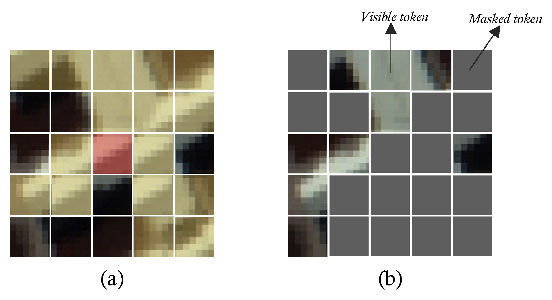
Figure 4.
Suppose the image above is a HSI patch. (a) Illustration of local homogeneity. The red pixel is the target pixel, the yellow area is made of the similar material as the target pixel. (b) Illustration of visible token and mask token.
Figure 4.
Suppose the image above is a HSI patch. (a) Illustration of local homogeneity. The red pixel is the target pixel, the yellow area is made of the similar material as the target pixel. (b) Illustration of visible token and mask token.
Local homogeneity is widespread in natural imagery. In the analysis of HSIs, to expand the amount of input information to enhance the performance of model, the neighborhood surrounding the target pixel is used as the network input. Yet, quite a bit more semantic redundancy comes with this strategy. Inspired by He Kaiming’s work, we randomly mask the input data to destroy its local homogeneity. After that, it conducts representation learning and reconstructs the original input that had been unmasked via an autoencoder. In this way, the model can implicitly learn the context and texture features in natural images.
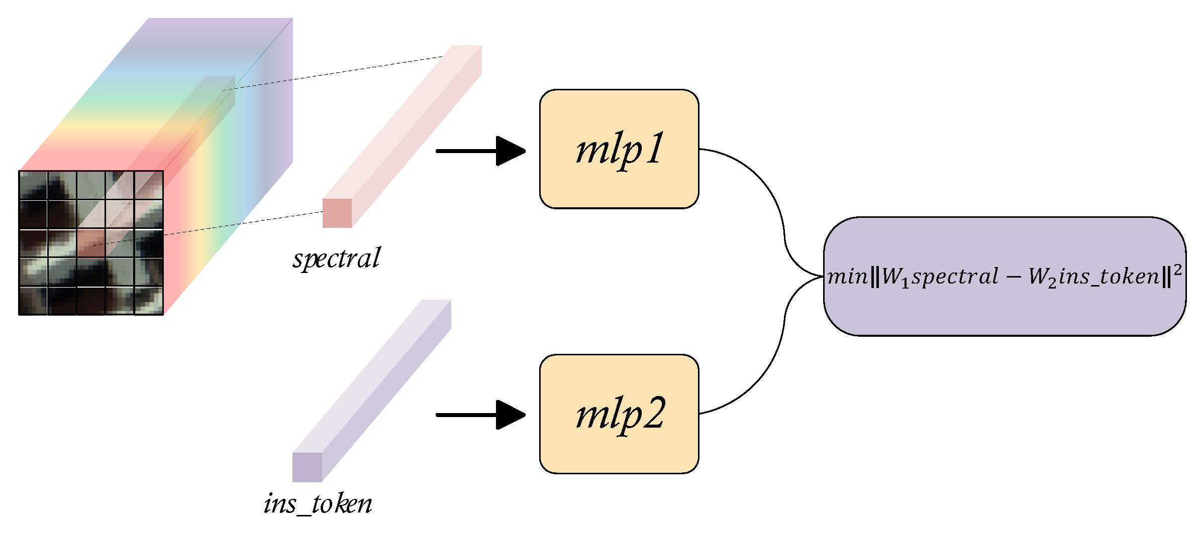
Regrettably, since the transformer model performs indiscriminate global self-attention calculations on input tokens, lacks inductive bias, has a broad function domain, and disperses local attention, training the transformer network requires a large amount of data. Considering that we are primarily interested in the relationship between the target pixel and its neighborhood with regard to HSIs analysis. In order to guide the model to prefer learning the information that is strongly related to the target pixel in the global information, so that the model can naturally focus on the area of human interested in. We introduce a randomly initialized instructor token, similar to
in ViT, to represent the general features of the input, called the
. Subsequently, minimize the distance between the projected vectors by mapping the output of decoder that corresponding to
and the spectral vector target pixel to a certain metric space. This instructing term can be regarded as a regularization constraint of the autoencoder that encourages the model to learn human prior knowledge of HSIs implicitly while decreasing the quantity of training data needed. Its working mechanism is shown in the
Figure 5.
Specifically, after the spatial-spectral embedding
, we random mask and flatten
, then contact the
to it as the input of encoder
. Let
represents the latent features of
.
Afterwards, we move the visible token to its original position, and then fill the masked token with a random token, called
.
Finally, we use
as the input of decoder to reconstruct the original HSI patch
as well as conduct instruction.
where
represents the center pixel. The loss function of the pretraining stage is:
2.4. Learnable aggregation
In downstream task, in order to make full use of the information learned by the network, we propose a learnable aggregation to combine the tokens from the encoder and then feed its outputs to the classifier as the final logit for supervised training. Specifically, we use the uncovered patch
as model input in forward propagation. Let the output of encoder
, the final
can compute as follow equations:
Where
f and
g represent MLP mapping,
b represents the spectral bands of input,
d represents the embedding dimension of encoder.
Finally, we employ the CrossEntropy loss function to train the classifier,as shown in equation
21.
Where
represents the parameters of model,
y represents the ground-truth of training data,
y represents the number of training data.
3. Experiment Results and Analysis
3.1. Datasets Description
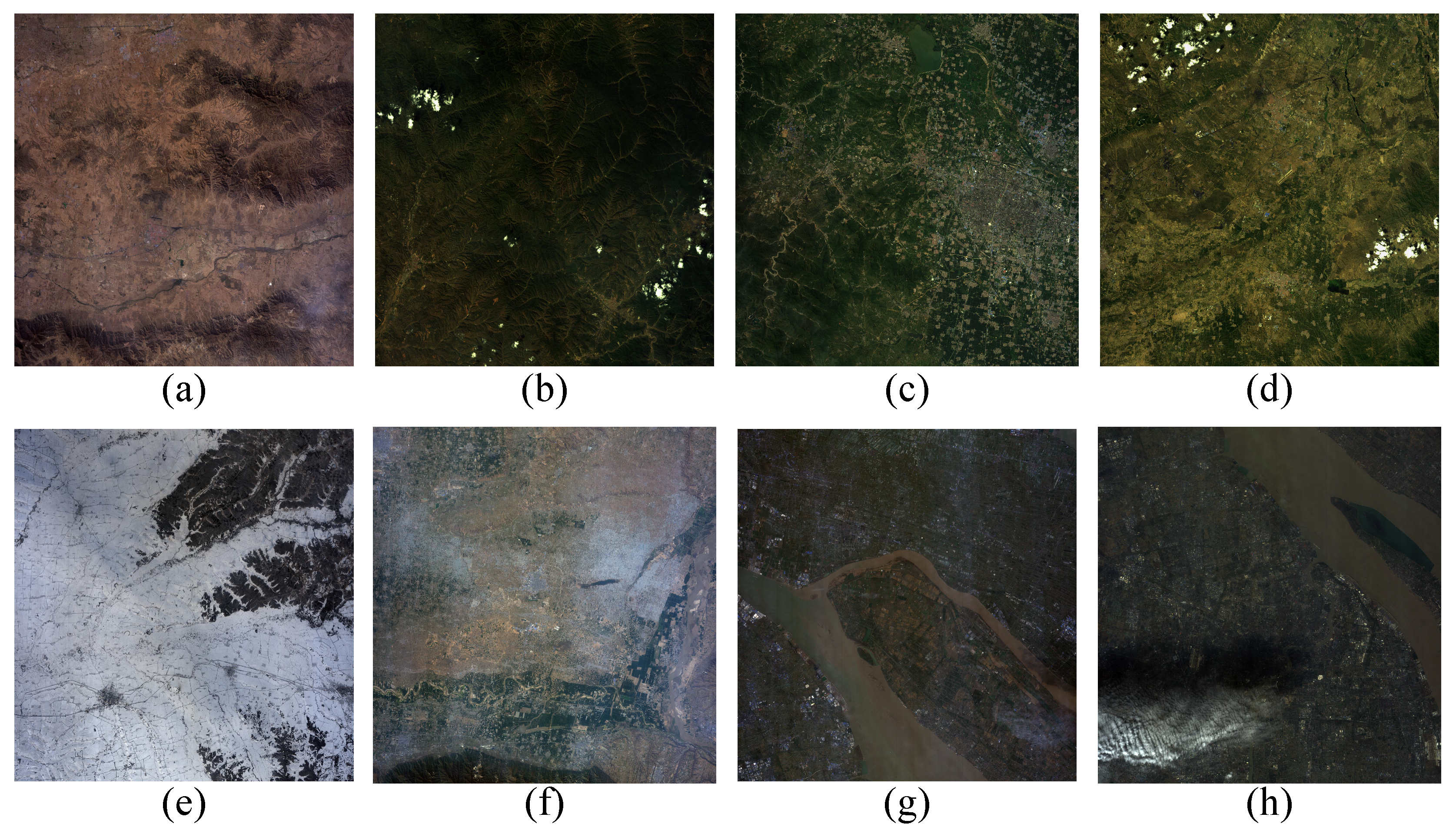
In pertraining stage, we selected hyperspectral images from a variety of scenes, including desert, forest, township, forest village, snowfield, village, city, metropolis, and divided them into four patches of varying size, 9, 15, 29, 33 respectively. These HSIs were gathered by GaoFen-5 satellite which contain 330 spectral bands in the wavelength range –m. The spectral resolution of VNIR and SWIR are 10nm and 20nm respectively. The size of each hyperspectal image is and the spatial resolution of these data is 30m peer pixel. 33 water absorption bands are removed in the process of data preprocessing.
Figure 6.
The false-color images of GaoFen-5 pretraining dataset. (a) Desert; (b) Forest; (c) Township; (d) Forest Village; (e) Snowfield; (f) Village; (g) City; (h) Metropolis.
Figure 6.
The false-color images of GaoFen-5 pretraining dataset. (a) Desert; (b) Forest; (c) Township; (d) Forest Village; (e) Snowfield; (f) Village; (g) City; (h) Metropolis.
After pertraining, the performance of the proposed method is evaluated on three widely-used hyperspectral datasets, including Indian Pines, Pavia University, and Salinas.
Indian Pines. The Indian Pines data set contains 145×145 pixels which gathered by the AVIRIS sensor in Northwestern Indiana, where AVRIS stands for airborne visible infrared imaging spectrometer. The original Indian Pines data set contains 220 spectral channels in the wavelength range from –m with a spatial resolution of 20m. In this paper, 20 bands corrupted by water absorption effects are discarded. It contains 16 classes and 42776 labeled pixels in total.
PaviaU. The University of Pavia data set contains 610 × 340 pixels collected by the ROSIS sensor at the University of Pavia, where ROSIS stands for reflective optics system imaging spectrometer. This image scene contains 103 spectral bands in the wavelength range from –m with a spatial resolution of 1.3 m. The data set was provided by Prof. Paolo Gamba from the Telecommunications and Remote Sensing Laboratory, University of Pavia. It contains 9 classes and 42776 labeled pixels in total.
Salinas. The Salinas dataset contains 512×217 pixels also collected by the AVIRIS sensor over Salinas Valley, California. These data contain 224 spectral bands range from –m with a spatial resolution of 3.7m. It contains 16 classes and 50929 labeled pixels in total.In this paper, 20 water absorption bands (108–112, 154–167, and 224) are removed during data preprocessing.
In our experiment, the characters of GaoFen5 Pretrained Dataset are all different from India Pians, PaviaU as well as Salinas. Thus, evaluating the classification performance of proposed method on these three widely used datasets can also test its generalization ability. The descriptions of all the datasets are summarized in
Table 4 and the false-color images and groundtruth of three widely used datasets are illustrated in
Figure 7.
Figure 7.
The false-color images and groundtruth of three widely used dataset. (a) The false-color images of Salinas; (b) The groundtruth of Salinas; (c) The false-color images of PaviaU; (d) The groundtruth of PaviaU; (e) The false-color images of Indian Pines; (f) The groundtruth of Indian Pines.
Figure 7.
The false-color images and groundtruth of three widely used dataset. (a) The false-color images of Salinas; (b) The groundtruth of Salinas; (c) The false-color images of PaviaU; (d) The groundtruth of PaviaU; (e) The false-color images of Indian Pines; (f) The groundtruth of Indian Pines.
Table 1.
Land cover classes illustration and numbers of training and testing samples for India Pines.
Table 1.
Land cover classes illustration and numbers of training and testing samples for India Pines.
| No. |
Class |
Training samples |
Testing samples |
Total samples |
| 1 |
Alfalfa |
20 |
26 |
46 |
| 2 |
Corn-notill |
20 |
1408 |
1428 |
| 3 |
Corn-mintill |
20 |
810 |
830 |
| 4 |
Corn |
20 |
217 |
237 |
| 5 |
Grass-pasture |
20 |
463 |
483 |
| 6 |
Grass-trees |
20 |
710 |
730 |
| 7 |
Grass-pasture-mowed |
14 |
14 |
28 |
| 8 |
Hay-windrowed |
20 |
450 |
478 |
| 9 |
Oats |
10 |
10 |
20 |
| 10 |
Soybean-notill |
20 |
952 |
972 |
| 11 |
Soybean-mintill |
20 |
2435 |
2455 |
| 12 |
Soybean-clean |
20 |
573 |
593 |
| 13 |
Wheat |
20 |
185 |
205 |
| 14 |
Woods |
20 |
1245 |
1265 |
| 15 |
Buildings-Grass-Trees |
20 |
366 |
386 |
| 16 |
Stone-Steel-Towers |
20 |
73 |
93 |
| |
Total |
304 |
9945 |
10249 |
Table 2.
Land cover classes illustration and numbers of training and testing samples for Salinas.
Table 2.
Land cover classes illustration and numbers of training and testing samples for Salinas.
| No. |
Class |
Training samples |
Testing samples |
Total samples |
| 1 |
Broccoli green weeds 1 |
20 |
1989 |
2009 |
| 2 |
Broccoli green weeds 2 |
20 |
3726 |
3726 |
| 3 |
Fallow |
20 |
1956 |
1976 |
| 4 |
Fallow rough plow |
20 |
1374 |
1394 |
| 5 |
Fallow smooth |
20 |
2658 |
2678 |
| 6 |
Stubble |
20 |
3939 |
3959 |
| 7 |
Celery |
20 |
3559 |
3579 |
| 8 |
Grapes untrained |
20 |
11251 |
11271 |
| 9 |
Soil vineyard develop |
20 |
6183 |
6203 |
| 10 |
Corn senesced green weeds |
20 |
3258 |
3278 |
| 11 |
Lettuce romaine 4 wk |
20 |
1048 |
1068 |
| 12 |
Lettuce romaine 5 wk |
20 |
1907 |
1927 |
| 13 |
Lettuce romaine 6 wk |
20 |
896 |
916 |
| 14 |
Lettuce romaine 7 wk |
20 |
1050 |
1070 |
| 15 |
Vineyard untrained |
20 |
7248 |
7268 |
| 16 |
Vineyard vertical trellis |
20 |
1787 |
1807 |
| |
Total |
320 |
50609 |
50929 |
Table 3.
Land cover classes illustration and numbers of training and testing samples for PaviaU.
Table 3.
Land cover classes illustration and numbers of training and testing samples for PaviaU.
| No. |
Class |
Training samples |
Testing samples |
Total samples |
| 1 |
Asphalt |
20 |
6611 |
6631 |
| 2 |
Meadows |
20 |
18629 |
18649 |
| 3 |
Gravel |
20 |
2079 |
2099 |
| 4 |
Trees |
20 |
3044 |
3064 |
| 5 |
Mental sheets |
20 |
1325 |
1345 |
| 6 |
Bare soil |
20 |
5009 |
5029 |
| 7 |
Bitumen |
20 |
1310 |
1330 |
| 8 |
Bricks |
20 |
3662 |
3682 |
| 9 |
Shadow |
20 |
927 |
947 |
| |
Total |
180 |
42596 |
42776 |
| Dataset |
Sensor |
Bands |
Spatial Resolution |
Classes |
Acquisition Year |
| GaoFen-5 |
AHSI |
330 |
30m |
- |
2019 |
| Indian Pines |
AVIRIS |
200 |
20m |
16 |
1992 |
| PaviaU |
ROSIS |
103 |
1.3m |
9 |
2001 |
| Salinas |
AVIRIS |
204 |
3.7m |
16 |
1998 |
3.2. Training Details and Experiment Settings
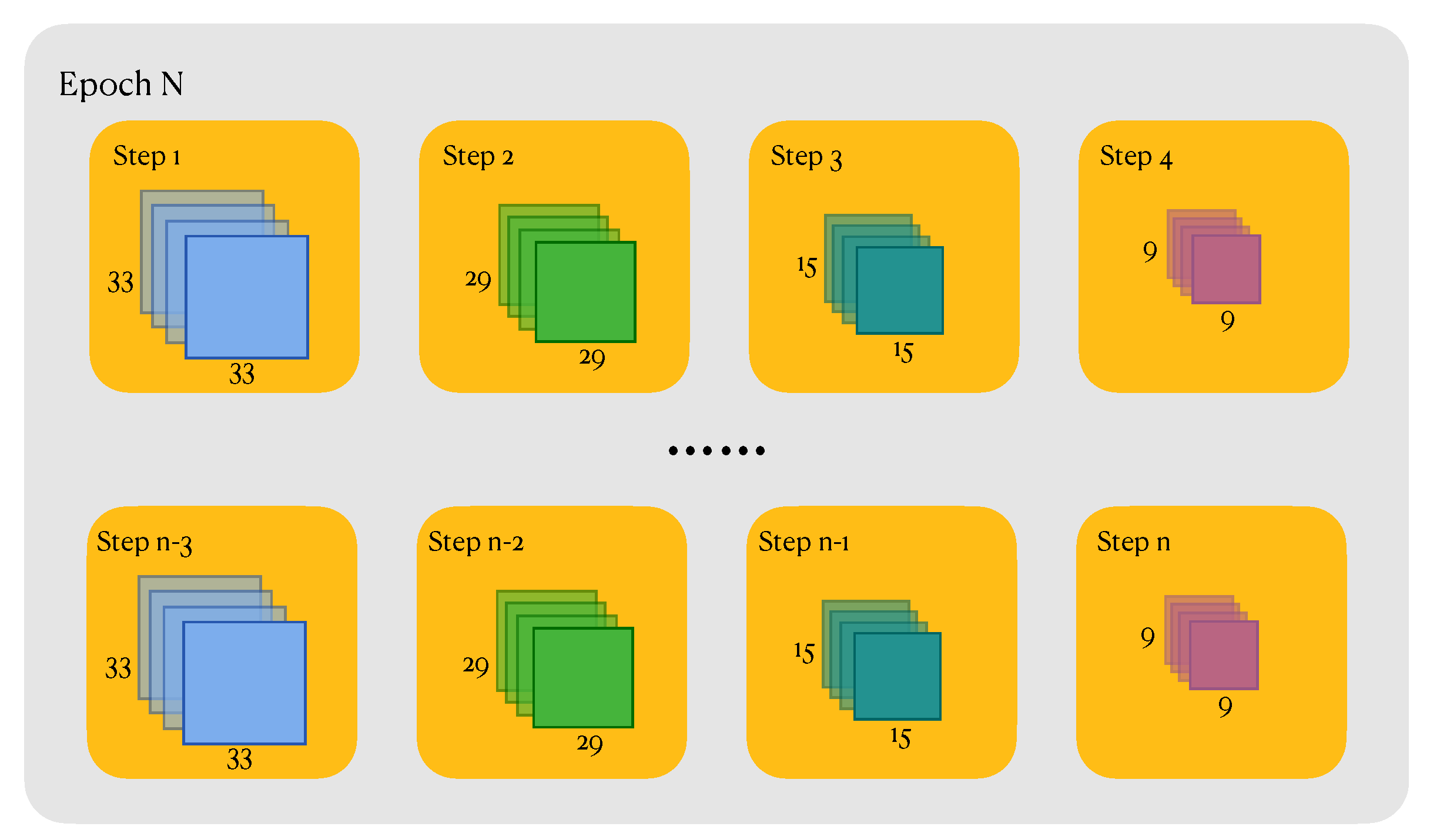
In the pre-training phase, the HSIs in GaoFen-5 Dataset are sliced into samples with 4 divergent sizes, 9, 15, 29, 33 respectively. Samples of the same size are uncovered.(For instance, suppose the size of HSI is , we divide it into patches with two different sizes, 10, 20 respectively. Consequently, the number of samples with size 10 is 100, the number of samples with size 20 is 25.) To compensate for the discrepancy in the number of samples of different sizes, we resample samples of larger size to align the number of samples of different sizes, hence eliminating the model’s bias with regard to the input sample size. After aligning, the number of total samples is about 300 thousand.
Mini-batch training strategy was employed during the training processing. Besides, we designed a custom dataloader, when sampling from dataset, each step in each epoch has a separate size, so as to guarantee that the model will be not biased by the sizes of samples. As illustrated in
Figure 8.
During the fine-tuning stage, 20 samples per class were random selected as the training data. In case a certain class has less than 40 samples, 50% of them are assigned as training data. Details of the data assignments can be found in
Table 1 and
Table 2. Given that the number of spectral bands in the downstream task’s data differs from that of the pre-trained network, we have to substitute the input layer of the trained IMAE encoder with an alternative input layer that can adapt to the new hyperspectral data. Otherwise, the network is unable to execute matrix operations due to dimension mismatch. Subsequently, as presented in
section 2.4, we aggregate the output tokens of encoder and submit the output feature vectors to a randomly initialized classifier for supervised classification training.
The implementation of our method is very sample which is completed entirely on PyTorch platform. In pretraining stage, a server with two A40 computing cards and 256GB memory was employed as the hardware platform; the mask ratio, embedding dimension, depth and heads of encoder were set to 0.5, 256, 4, 8 respectively, the parameters of decoder was half of it. AdamW was utilized as optimizer, the learning rate was set to . In downstream task, we use a terminal with a RTX3090 graphics card and 56GB memory as the computing platform; the learning rate of encoder and classifier were set to and respectively.
In order to quantify the classification performance of our method, the overall accuracy (OA), average accuracy (AA) and kappa coefficient (Kappa) were employed as evaluation measures. OA is the ratio of the number of correctly labeled hyperspectral pixels to the total number of hyperspectral pixels in test samples. AA is the mean of accuracy in different land-cover categories. Kappa measures the consistency between classification results and ground truth. The larger values of OA, AA, and Kappa represent the better classification results.
3.3. Validity Estimate
The generalization performance of the model is the core metric of our method. In this section, we first test the reconstruction ability of the pertrained model. Afterawards we are going to assess the generalizability of IMAE, from the perspective of training and inference of downstream tasks. Finally, we analyze the influence of pre-trained weights on model convergence speed.
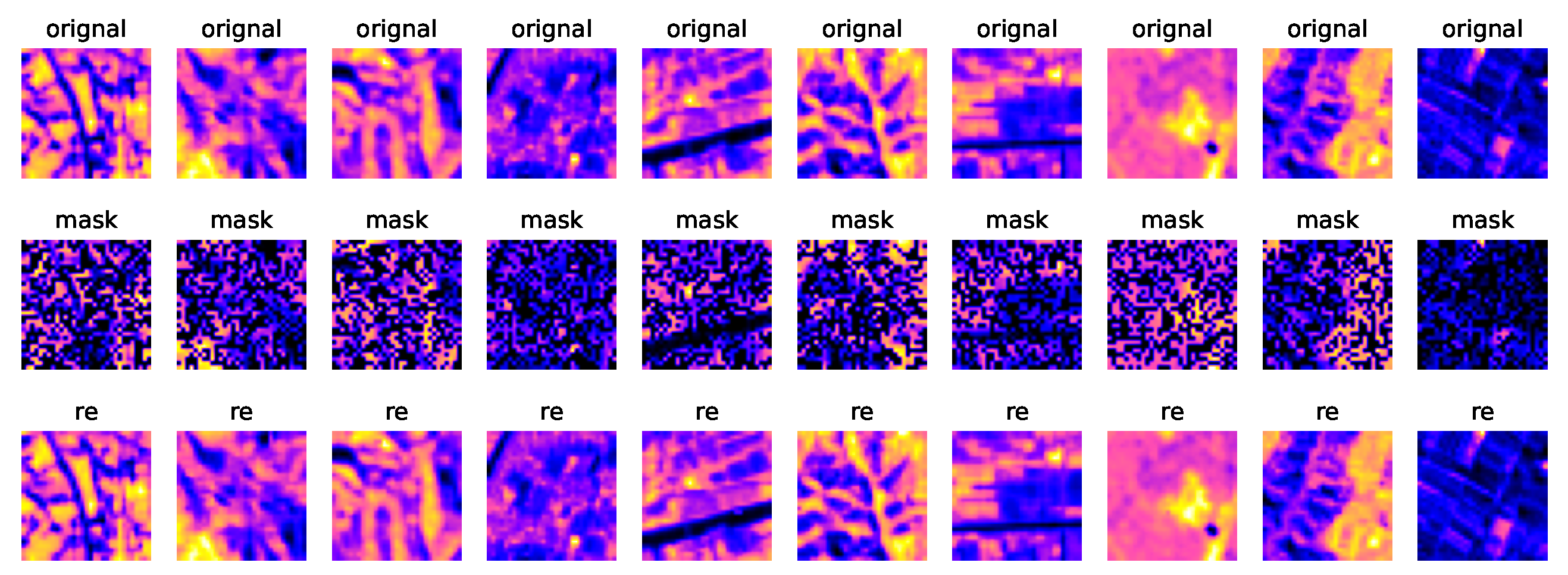
As above mentioned, we random mask 50% hyperspectral image samples, then reconstruct it to the original samples through a transformer based autoencoder. PSNR and SSIM are employed to evaluate the reconstruction performance. The average value of PSNR and SSIM on test set are
50dB and
0.99 respectively, which means the latent knowledge of HSI was fully learnt by our model, and the overfitting did not take place.
Figure 9 shows the original samples, masked samples and reconstructed samples.
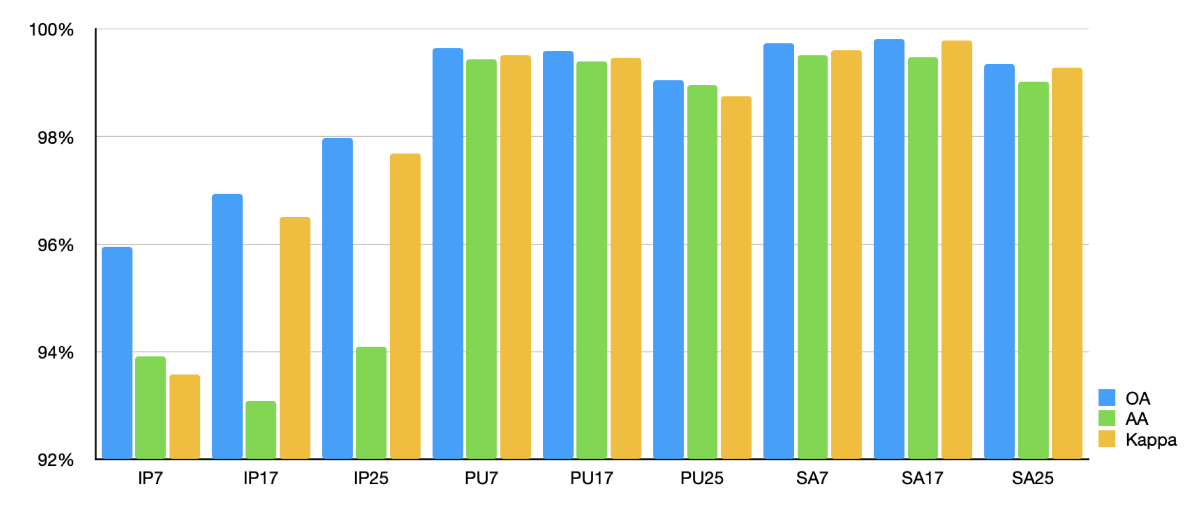
In the pertrained stage, IMAE was trained by HSI samples with 4 different sizes namely 33, 29, 15, 9. To examine the generation capacity of our pretrained model on the sample size, we random seleced 10% samples of per class in three widely used datasets with 3 different sizes which are distinct from it in the pretraining dataset. The classification results are shown in
Figure 10.
It is evident that despite the fact that the size and spectral resolution of the training data in the downstream tasks are not consistent with those in the pretraining dataset, our method still achieves excellent classification results on these data.
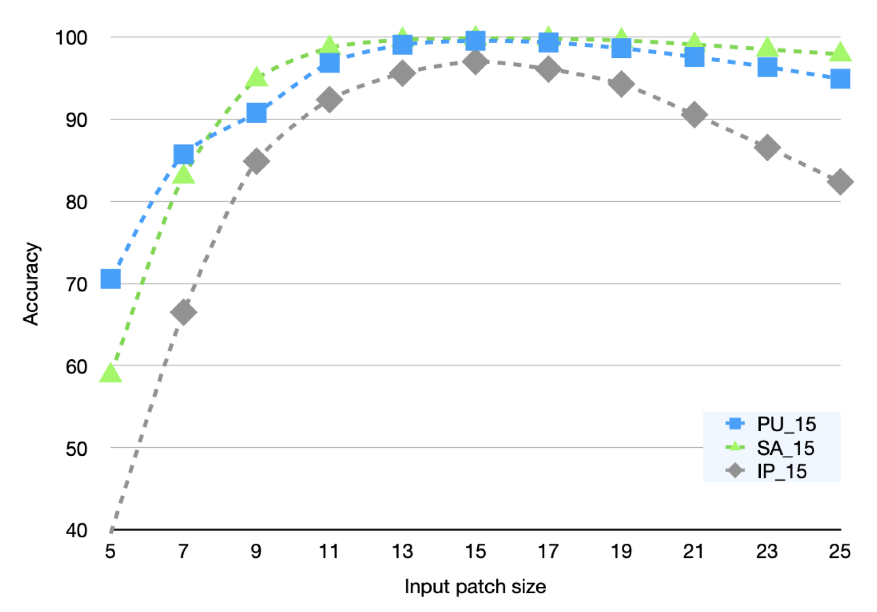
In the inference stage, we only fine-tune on the training set with a sample size of 15. Then, we evaluate the classification accuracy of our inferences using samples whose sizes differ from those in the training set. The experiment result is illustrated in
Figure 11.
Obviously, the common feature of the three curves in
Figure 11 is that When the input sample size is small, the inference accuracy is also small. As the input sample size increases, the inference accuracy also increases sharply until the inference sample size is equal to the training sample size. The inference accuracy gradually declines as the inference sample is larger than the training sample. We postulate that the reason for this phenomenon is that when the input sample size is small, the model is unable to learn enough contextual information, leading to low inference accuracy; when the input sample size is large, due to the presence of
, the model prefers to focus on areas close to the center pixel, allowing the model to suppress invalid information brought on by the increase in input sample size, thereby lessening the impact on inference accuracy.
In classification task, as the
Figure 12 shown, our method can greatly improve the performance and speed up the convergence rate especially when the training data is relatively small. By observing the curves in the figure we find that training with randomly initialized weights converges slowly on PU and SA, and it not converges on IN. When pre-trained weights were used for training, however, it significantly accelerated convergence on SA and PU datasets and really converged on the IN dataset, and its accuracy was equivalent to some start-of-the-art methods. We only replaced an input layer!
3.4. Classification Results
To verify the advancement of the our method, we compared the classification results with SVM, RNN, 3D-CNN, VIT, HIT, MAEST, SSTN and SS-MTr. Among these comparative methods, SVM is a classic machine learning method. RNN and 3D-CNN are mainstream deep learning methods. VIT, HIT and SSTN are Transformer-based methods, in particular, VIT is the first Transformer-based model used for image processing. HIT and SSTN have implemented some improvements on its basis to make it more suitable for HSI classification tasks. Similar to our method, MAEST and SS-MTr are pre-training methods with backbone network as MAE. The training data assignments for all compared methods as same as IMAE; the size of the input samples for CNN-based and transformer-based methods was set to 15×15.
Table 5,
Table 6 and
Table 7 record the classification results of different methods on Inidan Pine, PaviaU and Salinas dataset, including accuracy for each class and OA, AA, Kappa for all classes.
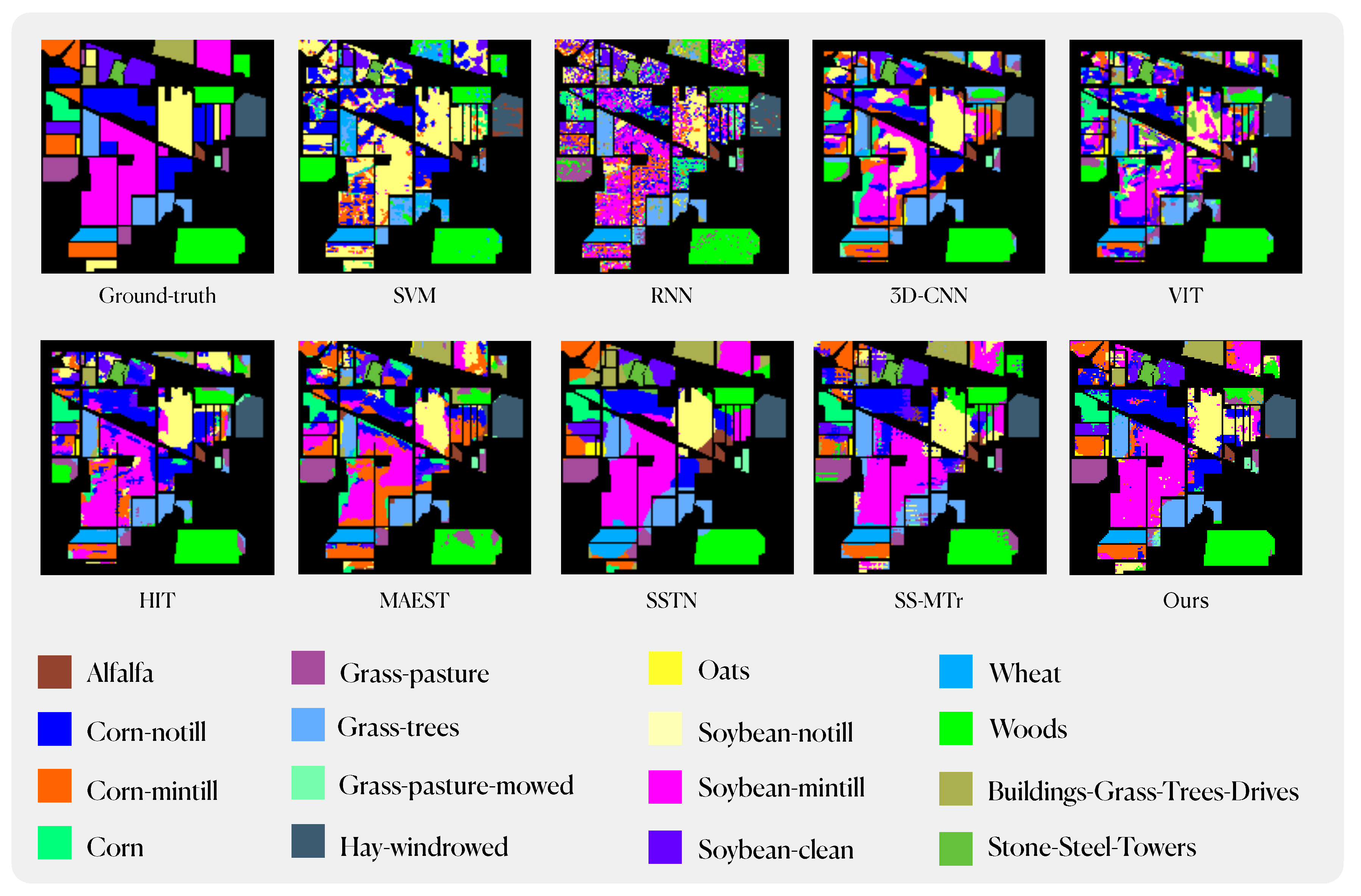
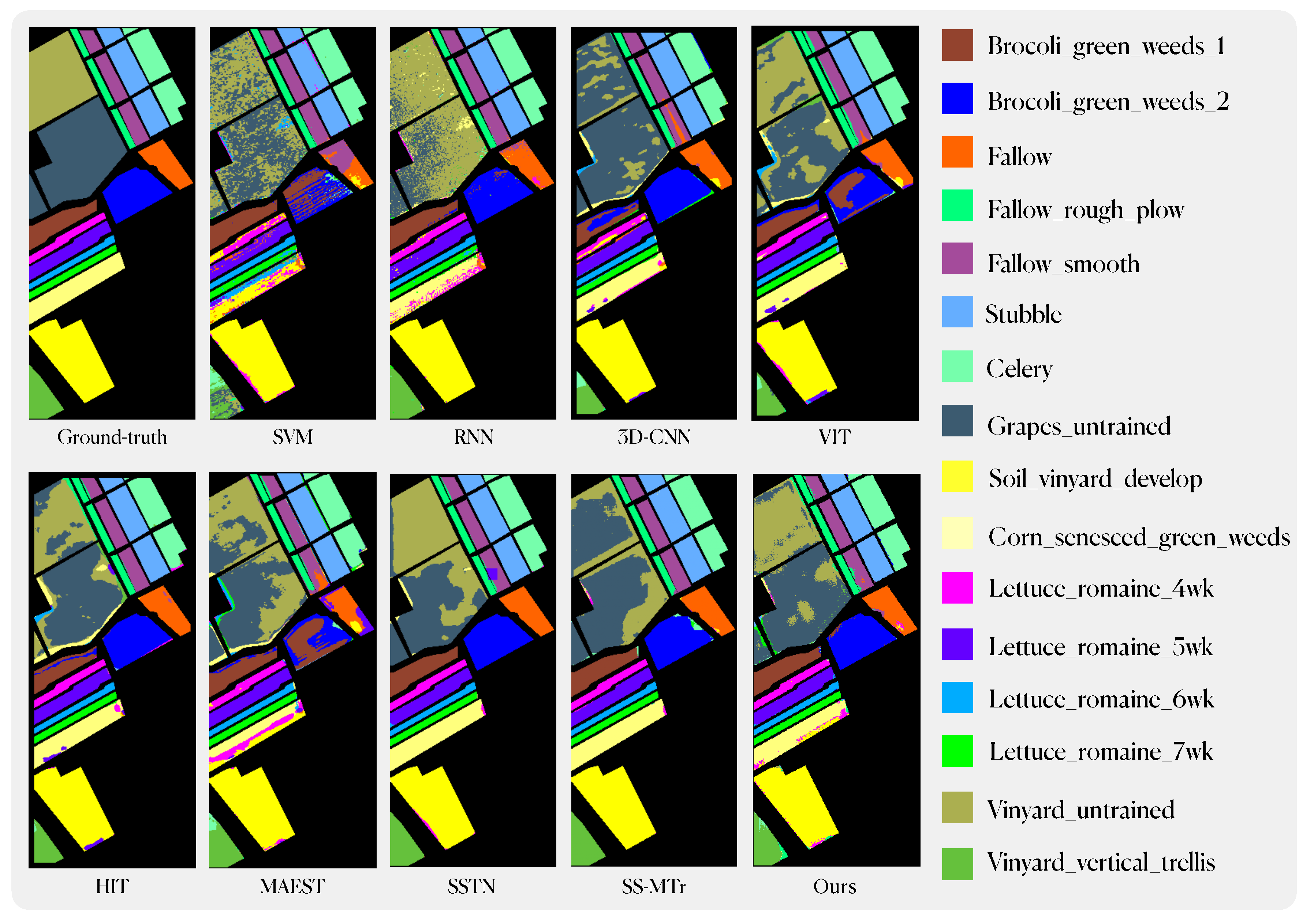
Figure 13,
Figure 14 and
Figure 15 illustrate the classification maps of different methods. Based on the empirical evidence derived from our experiments, it becomes apparent that traditional machine learning and deep learning algorithms struggle to perform effectively in scenarios marked by a paucity of available samples. Even the original ViT model yields suboptimal results. This phenomenon can be attributed to the fact that classical machine learning algorithms exhibit limited feature extraction capabilities, particularly when confronted with the intricate nature of hyperspectral imagery, thereby constraining their capacity for accurate classification. Mainstream deep learning algorithms, owing to the intricate complexity of their architectures, necessitate a substantial volume of data for successful model fitting. Consequently, their performance tends to degrade notably when dealing with datasets comprising as few as 20 samples per class or even fewer, frequently leading to severe overfitting issues. ViT, as a model grounded in the Transformer architecture and devoid of specific inductive biases, paradoxically exhibits reduced performance compared to CNN-based models when faced with limited sample availability, due to its greater data requirements. In contrast, enhanced Transformer-based networks, often incorporating convolutional networks at the input layer, exhibit substantially improved feature extraction capabilities. Beyond achieving translational invariance, these models also excel at capturing long-range contextual information, thereby markedly enhancing their performance in settings characterized by limited training sample numbers. Lastly, pre-trained networks akin to ours, which mitigate data requirements through pre-training, have demonstrated commendable performance. Nevertheless, limitations imposed by their model architecture and training strategies hinder their ability to exploit extensive pools of unlabeled data for pre-training, leaving room for further enhancement.
Table 5.
Classification results of different methods using 20 training samples per class on Indian Pines Dataset.
Table 5.
Classification results of different methods using 20 training samples per class on Indian Pines Dataset.
| Classes |
SVM |
RNN |
3D-CNN |
VIT |
HIT |
MAEST |
SSTN |
SS-MTr |
Ours |
| 1 |
97.83% |
84.78% |
97.83% |
91.3% |
95.65% |
100% |
100% |
96.15% |
95.65% |
| 2 |
47.76% |
30.74% |
35.64% |
35.85% |
66.32% |
41.81% |
57.29% |
72.51% |
75.35% |
| 3 |
10.12% |
31.45% |
36.39% |
19.88% |
35.06% |
66.27% |
49.76% |
78.40% |
74.22% |
| 4 |
17.72% |
63.71% |
44.73% |
64.98% |
81.86% |
76.79% |
93.25% |
97.24% |
98.31% |
| 5 |
0% |
62.32% |
13.25% |
25.47% |
39.75% |
87.37% |
80.12% |
77.32% |
81.16% |
| 6 |
39.86% |
85.34% |
79.45% |
63.97% |
88.63% |
84.11% |
88.9% |
99.15% |
92.47% |
| 7 |
0% |
92.86% |
100% |
100% |
100% |
96.43% |
100% |
100% |
96.43% |
| 8 |
80.75 |
88.28% |
89.96% |
85.98% |
85.77% |
98.95% |
99.79% |
100% |
98.54% |
| 9 |
0% |
85% |
100% |
100% |
100% |
100% |
80% |
100% |
100% |
| 10 |
74.07% |
44.96% |
59.88% |
35.49% |
64.71% |
57.10% |
66.36% |
87.5% |
76.13% |
| 11 |
1.87% |
38.7% |
34.50% |
38.04% |
55.11% |
43.14% |
88.47% |
69.86% |
86.03% |
| 12 |
22.09% |
52.45% |
41.15% |
32.04% |
51.77% |
31.53% |
70.49% |
72.95% |
72.68% |
| 13 |
99.51% |
98.05% |
77.56% |
98.54% |
96.59% |
99.51% |
98.54% |
100% |
99.51% |
| 14 |
94.31% |
88.30% |
74.23% |
79.76% |
83.72% |
72.72% |
92.17% |
91.97% |
85.77% |
| 15 |
3.37% |
48.19% |
23.83% |
31.87% |
43.01% |
81.34% |
100% |
95.08% |
95.60% |
| 16 |
90.32% |
96.77% |
100% |
93.55% |
98.92% |
97.84% |
100% |
100% |
100% |
| OA |
38.26% |
54.36% |
49.18% |
46.95% |
64.17% |
61.09% |
79.39% |
81.82% |
83.79% |
| AA |
42.47% |
68.24% |
63.02% |
62.30% |
74.18% |
77.18% |
85.32% |
89.88% |
89.24% |
| Kappa |
32% |
49.21% |
44.17% |
41.37% |
59.98% |
56.76% |
76.8% |
79.45% |
81.60% |
Table 6.
Classification results of different methods using 20 training samples per class on Salinas Dataset
Table 6.
Classification results of different methods using 20 training samples per class on Salinas Dataset
| Classes |
SVM |
RNN |
3D-CNN |
VIT |
HIT |
MAEST |
SSTN |
SS-MTr |
Ours |
| 1 |
99.65% |
97.31% |
54.95% |
74.51% |
79.24% |
90.69% |
100% |
98.59% |
99.15% |
| 2 |
48.66% |
96.56% |
96.46% |
64.04% |
97.80% |
43.26% |
99.97% |
95.84% |
97.58% |
| 3 |
40.79% |
87.35% |
92.86% |
85.98% |
96.96% |
65.64% |
99.9% |
97.96% |
92.76% |
| 4 |
98.78% |
98.78% |
90.32% |
95.98% |
96.56% |
93.97% |
99.14% |
97.89% |
99.57% |
| 5 |
97.98% |
98.77% |
88.87% |
80.77% |
95.33% |
81.07% |
89.32% |
100% |
94.88% |
| 6 |
96.84% |
99.49% |
95.33% |
95.38% |
95.38% |
97.42% |
99.97% |
99.92% |
99.72% |
| 7 |
98.60% |
99.69% |
91.95% |
95.39% |
93.66% |
95.95% |
99.78% |
99.75% |
98.97% |
| 8 |
62.31% |
33.86% |
83.44% |
65.84% |
72.62% |
61.76% |
68.32% |
70.3% |
85.18% |
| 9 |
95.81% |
99.85% |
97.79% |
93.36% |
96.5% |
98.61% |
97.94% |
99.98% |
97.10% |
| 10 |
1.98% |
70.44% |
81.94% |
88.87% |
86.15% |
45.85% |
98.54% |
98.68% |
80.29% |
| 11 |
66.10% |
91.39% |
69.94% |
87.83% |
93.07% |
96.16% |
100% |
100% |
98.69% |
| 12 |
88.69% |
98.65% |
88.22% |
93.15% |
92.79% |
100% |
98.86% |
98.32% |
98.24% |
| 13 |
99.02% |
99.02% |
93.23% |
93.45% |
94.21% |
98.14% |
100% |
100% |
98.91% |
| 14 |
88.22% |
91.50% |
88.13% |
91.21% |
94.02% |
99.44% |
99.44% |
100% |
100% |
| 15 |
65.63% |
87.08% |
22.43% |
72.34% |
64.72% |
66.39% |
96.87% |
30.81% |
85.66% |
| 16 |
41.84% |
97.51% |
57.44% |
60.71% |
65.58% |
90.81% |
99.89% |
100% |
89.71% |
| OA |
71.70% |
81.25% |
78.16% |
80.03% |
84.45% |
76.61% |
91.76% |
83.84% |
92.20% |
| AA |
74.43% |
90.45% |
80.83% |
83.68% |
88.41% |
82.82% |
96.62% |
93% |
94.78% |
| Kappa |
68.53% |
79.37% |
75.69% |
82.86% |
82.86% |
74.11% |
90.88% |
81.96% |
91.34% |
Table 7.
Classification results of different methods using 20 training samples per class on PaviaU Dataset
Table 7.
Classification results of different methods using 20 training samples per class on PaviaU Dataset
| Classes |
SVM |
RNN |
3D-CNN |
VIT |
HIT |
MAEST |
SSTN |
SS-MTr |
Ours |
| 1 |
61.02% |
51.95% |
63.17% |
67.26% |
53.55% |
70.68% |
71.62% |
90.15% |
95.34% |
| 2 |
70.57% |
47.36% |
66.89% |
61.67% |
82.34% |
76.14% |
98.04% |
74.66% |
92.92% |
| 3 |
16.15% |
29.25% |
55.60% |
58.89% |
36.11% |
72.89% |
87.28% |
90.52% |
90.33% |
| 4 |
96.70% |
90.05% |
81.46% |
85.93% |
92.20% |
89.46% |
58.02% |
85.48% |
89.85% |
| 5 |
99.11% |
99.11% |
85.50% |
100% |
99.85% |
99.78% |
100% |
99.40% |
99.26% |
| 6 |
33.27% |
34.86% |
64.94% |
80.71% |
46.25% |
80.97% |
92.42% |
91.08% |
80.49% |
| 7 |
95.26% |
98.50% |
78.65% |
77.82% |
89.10% |
87.44% |
100% |
99.01% |
89.47% |
| 8 |
81.72% |
48.18% |
70.56% |
89.33% |
62.49% |
79.44% |
87.05% |
85.94% |
87.62% |
| 9 |
72.63% |
99.05% |
92.19% |
92.93% |
99.26% |
99.89% |
39.5% |
91.80% |
93.24% |
| OA |
67.18% |
53.20% |
68.40% |
71.16% |
71.50% |
78.56% |
87.78% |
84.95% |
91.13% |
| AA |
72.63% |
66.48% |
73.22% |
79.39% |
73.46% |
84.08% |
81.55% |
89.78% |
90.95% |
| Kappa |
58.10% |
44.52% |
60.55% |
64.66% |
63.22% |
72.7% |
83.78% |
80.91% |
88.28% |
Figure 13.
Classification maps using different methods on the Indian Pines dataset.
Figure 13.
Classification maps using different methods on the Indian Pines dataset.
Our method has achieved state-of-the-art performance under equivalent experimental conditions. Specifically, on the IN dataset, we attained an Overall Accuracy (OA) of 83.79%, an Average Accuracy (AA) of 89.24%, and a Kappa coefficient of 81.60%. Similarly, on the SA dataset, our model achieved an OA of 92.2%, an AA of 94.78%, and a Kappa of 91.34%. On the PU dataset, our performance metrics were recorded at 91.13% for OA, 90.95% for AA, and 88.28% for Kappa. Across these three datasets, our model outperforms traditional machine learning and deep learning methods by a substantial margin. In comparison to the enhanced ViT model, our approach, including the best-performing model SSTN within it, exhibits notable improvements across various performance indicators. Furthermore, in comparison to similar pre-training methods, our model surpasses MAEST in terms of AA, OA, and Kappa on all datasets. Compared to SS-MTr, except for the Indian Pines dataset, where AA score of IMAE is on par with SS-MTr. In all other datasets, our model consistently outperforms SS-MTr across various performance metrics.
Figure 14.
Classification maps using different methods on the Salinas dataset.
Figure 14.
Classification maps using different methods on the Salinas dataset.
Figure 15.
Classification maps using different methods on the PaviaU dataset.
Figure 15.
Classification maps using different methods on the PaviaU dataset.
