Accelerated gradient-based algorithm combined with progressive Big-Bang to optimize the layout in offshore wind farms

Preprint

Article

Accelerated gradient-based algorithm combined with progressive Big-Bang to optimize the layout in offshore wind farms

Altmetrics

Downloads

Views

Comments

Angel Gaspar Gonzalez-Rodriguez^*

Juan Manuel Roldan-Fernandez

José Vicente Muñoz Díez

Angel Gaspar Gonzalez-Rodriguez^*

Juan Manuel Roldan-Fernandez

José Vicente Muñoz Díez

This version is not peer-reviewed

Submitted:

06 September 2023

Posted:

08 September 2023

You are already at the latest version

Alerts

Abstract

A new layout optimization method for offshore wind farms is proposed to minimize power deficits due to wake effect. The main engine of the algorithm is a gradient-descent method, in which an analogy is established between power deficit and repulsive electrostatic potential energy. To achieve a maximum dispersion in the initial solution, throughout the optimization process, new turbines are included in the centre of the concession area, and quickly expand outward looking for areas with less potential, in turn pushing the previous ones. When the optimization process ends, to avoid local maximums, it enters into a process of suppression of the set of locations that cause the greatest potential (power deficit). Then, a potential map of the entire area is created and a greedy algorithm includes new turbines to complete the layout with the final number of turbines. To speed up the search process and the creation of the potential map, two simplifications have been validated and added: the spatial distribution of velocities has been converted into its equivalent with point symmetry; and, for turbines affected by multiple wakes, the power deficit has been calculated by using a linear aggregation of powers, instead of the usual linear (or quadratic) aggregation of speeds. Owing to this type of aggregation, the process is accelerated in a factor of 90.

Keywords:

Subject: Engineering - Electrical and Electronic Engineering

1. Introduction

The problem of the distribution of turbines in offshore wind farms, also known as Offshore Wind Farms Layout Optimization Problem (OWFLOP) is the most important factor determining the wind speed deficit, and consequently, it strongly influences the generation of income from the sale of electrical energy. The five most important groups of optimization algorithm used for the OWFLOP are: heuristic, pattern search, simulated annealing, evolutionary algorithms and gradient search [1].

Table 1, taken from [2,3] presents a summary of previous works related to the aforementioned issue of the layout optimization, indicating the type of search engine. A more complete review was provided by [4], where most of the cases under study spin around random search algorithms, specially those using a Genetic Algorithm (GA). For most of them, the objective function to optimize is the Annual Energy Production (

A E P

), or correspondingly, the average farm power (

\bar{P}

From a thoughtful review of the literature concerning this matter is concluded that most of the research on the OWFLOP starts from a small and uniform rectangular space divided into columns and rows, forming a mesh of cells. Then, the algorithm decides whether locate a turbine in the centre of a cell or not. Obviously, a coarse lattice considerably limits the solution space for the turbine locations, while a sufficiently fine lattice increases cubically the computational cost of the algorithm execution process [5] given that the number of possible solutions is

N s o l = \frac{N c!}{n t! (N c - n t)!}

(1)

where

N c

is the number of cells and

n t

is the number of turbines.

Due to the high computational cost of these traditional techniques, most articles are reduced to 10x10 or 20x20 meshes. In [6], a collection of 46 articles with these characteristics is shown, many of them using algorithms based on animal behaviour (genetic algorithm, particle swarm, Harris hawk, elephant herding, cuckoo, algae), and mostly showing an artificial solution to the layout problem. All in all, the general trend is the use of meta-heuristic algorithms where the achievement of the optimum (in relation to the mathematical formulation of the problem) is not guaranteed, especially when the solution space is increased.

Gradient-based (GB) methods are often disregarded because of their poorer performance in terms of accuracy, since they are prone to fall in local maxima. Although they perform significantly well owing to their quick convergence features [7], some authors have pointed out that depending on the gradient calculation method, their computational time can be insurmountable for large offshore wind farms [8]. The calculation of the objective function in any type of optimization algorithm requires many operations, and in the case of using its gradient, even more. A finite-difference approximation of gradients (FDAG) with regards to the variables to be optimized (typically the x,y components of each turbine) entails tripling the number of operations necessary to estimate the

A E P

. Obtaining the gradient using analytical formulas, as in [9], takes a time that would slow down any search method given the high number of trigonometric, quadratic and inverse operations to perform.

The computation time can increase if, in addition, the Hessian matrix is calculated at each step. Guirguis, in [10], develops differentiable mathematical models to handle the Concession Area (CA) constraints, and compares the performance (for a interior point method) using FDAG and the exact gradients showing, for the former, significantly lower computation times at the expense of a negligible deviation in accuracy. The main problem is that introduces numerical errors that can affect the convergence of the algorithm, especially for highly constrained problems. This same author, in [11] compares a GB multi-objective algorithm to a NSGA-II, claiming the superiority of the former in terms of coverage, spread and computational cost.

Including spatial constrains in the search space is a design feature addressed in many other works related to the layout optimization. A solution for irregularly shaped and discontinuous polygons are also proposed in [12] by identifying the nearest edge and polygon, and in [13] by means of a dynamic penalty functions.

In other works where GB methods are used, they are often restricted to very local searches [14], or focused on a fine tuning of a heuristic algorithm [15,16].

Furthermore, the optimal location problem is not convex and GB methods may be unable to find the global optimum. Consequently, these methods are often combined with some other to escape from local maxima. In [8], triangulation is used as the starting point of the gradient method, with the additional idea of maximizing turbine dispersion, thus reducing maximum turbine loads. Quick et al in [17], uses a stochastic gradient descent, estimates the gradient of the

A E P

using Monte Carlo simulation, achieving lower computation times as long as the farm size is above 225 turbines.

This article presents a method whose search engine is a gradient-based optimization with the following improvements over traditional search:

Symmetry.: It will be verified that it is possible to substitute a wind distribution for its equivalent with point symmetry. This statement will lead to important simplifications in the evaluation of the power deficit.
Linearization.: When a turbine is immersed in the wakes of several upstream turbines there are several aggregation methods to obtain the resulting deficit. An additional aggregation method will be provided that will drastically simplify and speed up the computation of the objective function gradient, enabling the use of look-up tables.
Progressive Big Bang.: As a starting point, it is proposed to progressively incorporate turbines into the concession area from the centre, so that they are repelled towards the periphery, which is usually optimal for widespreading purposes. This causes a greater mobility of the turbines and a broader search in the concession area.
Greedy reposition of local maxima.: Turbines with higher power deficit will be reallocated to avoid local maxima.

In order to explain the method used for each tool, and its validation, the remaining of the article has been structured as follows:

Section 2. Brief formulation of the problem and equations for the $A E P$ deficit as objective function.
Section 3. Description and validation of the transformation into point symmetry for the wind direction distribution.
Section 4. Description and validation of the linear aggregation of the power deficit (LAPD).
Section 5. Method of gradient-based search, combined with the Progressive Big Bang (PBB).
Section 7. Limitations and consideration of the proposed method.

2. Annual energy produced by a wind farm

The general form for calculating the energy produced by a wind farm is obtained by adding together the average power,

{\bar{P}}_{i}

, produced by each of the

n t

turbines in the wind farm, for every wind direction and for every wind speed. In a year (T = 8766 h), the energy produced by the wind farm,

A E P

, can be obtained from:

A E P = T \sum_{i = 1}^{n t} {\bar{P}}_{i}

(2)

and

{\bar{P}}_{i} = \int_{u_{c i}}^{u_{c o}} \int_{0}^{2 π} P c (v_{i}) f_{v e l} (u) f_{d i r} (θ) d u d θ

(3)

where u is the free-flow wind speed,

u_{c i}

and

u_{c o}

are the cut-in speed and cut-out speed, respectively,

P c (u)

is the relation between the wind speed and the power (the power curve as given by the turbine manufacturer),

v_{i}

is the effective wind speed passing through the rotor turbine,

f_{v e l} (u)

is frequency with which he wind blows with speed u, and

f_{d i r} (θ)

is the probability that the wind comes from the direction

θ

In the case of a wind farm with

n t

turbines arranged in a certain layout, L, each turbine i can suffer the perturbation of other upstream turbines. Therefore, it is necessary to include in the expression above the power deficit resulting from these perturbations, which cause the effective speed of the air flow reaching the turbine i to be smaller than the free-stream wind speed (

v_{i} < u

This speed deficit

δ v_{i}

at turbine i depends on the turbine itself, on the free-stream wind speed u, its direction

θ

, and the layout L, that is

v_{i} = u - δ v with δ v_{i} = δ v (u, θ, i, L) and i \leq n t

(4)

For sake of space, expressions to calculate deficit are not included in this work, but can be followed at [18].

Two considerations can be taken into consideration for the previous expressions:

In fact, the upper limit of integration should be $u^{'}$ , with $u^{'} : u_{c o} = u^{'} - δ v (u^{'}, θ, i, L)$ , and that could be different for each turbine, direction and layout. Actually, and due to the infrequent occurrence of velocities close to $u_{c o}$ , the minor relevance of this distinction is intuited, and will be disregarded.
To be precise, this summation should be multiplied by the availability and losses factor, $k_{A L}$ ( $k_{A L} \leq 1$ ), that allows the designer to take into account the loss of production due to unavailability of turbines and other losses including: those that occur in the electrical installation or due to delays and errors in the turbine orientation; errors in the power curve of the turbine itself; or delays in turbine reconnection after a stop for exceeding the maximum speed (hysteresis). Obtaining the proper value of this parameter is not a trivial problem. For clarity, this factor will not be taken into account in the explanations, and can be recovered to obtain a more realistic result of the $A E P$ .

2.1. Discretizing the calculation of the annual energy produced by a turbine

In general, expression (3) is not analytically integrable, regardless of whether or not it is possible to obtain an analytic expression for the functions

P c (\cdot)

f_{v e l} (\cdot)

f_{d i r} (\cdot)

. Therefore, it has to be discretized, and the integratives turn into summations. It is usual to set

Δ u = 1 m / s

as the discretization step for the wind speed and

Δ θ = 1 deg

for its direction, yielding:

\bar{P} = \frac{A E P}{T} = \sum_{i = 1}^{N t} \sum_{v = u_{c i}}^{u_{c o}} \sum_{θ = 1}^{360} P c (v_{i}) f (u, θ) Δ u Δ θ with f (u, θ) = f_{v e l} (u) f_{d i r} (θ)

(5)

The energy deficit and average power deficit due to the wake effect result

\begin{matrix} δ \bar{P} = n t {\bar{P}}_{1 T} - \bar{P} \end{matrix}

(6)

\begin{matrix} δ A E P = T n t {\bar{P}}_{1 T} - A E P \end{matrix}

(7)

where

{\bar{P}}_{1 T}

is the average power produced by an isolated turbine under the same wind conditions:

{\bar{P}}_{1 T} = \sum_{u = u_{c i}}^{u_{c o}} P c (u) f_{v e l} (u) Δ u .

(8)

3. Symmetrization

In this section, the AEP deficit will be evaluated. The traditional method consists in estimating the energy for the entire range of wind directions by taking into account the probability in each direction. However, in this subsection it is proposed to consider only half of the range, taking as probability for an angle

θ

the sum of the original ones for

θ

and

θ + π

. Therefore, the expression(5) becomes the following one:

\bar{P} = \frac{A E P}{T} = \sum_{j = 1}^{N t} \sum_{v = u_{c i}}^{u_{c o}} \sum_{θ = 1}^{180} P c (v_{j}) (f (u, θ) + f (u, θ + π)) Δ u Δ θ .

(9)

Several tests have been carried out with different wind farms (see Figure 1) to check the deviation due to this simplification:

Horns Rev 1 (HR1), with uniform distribution in rows and columns, and hence point symmetry.
HR1 layout, but randomly displacing each turbine to convert the layout into a non-uniform one.
Horns Rev 2 (HR2), with uniform distribution but without point symmetry.
Anholt, irregular-shape OWF.

Wind conditions at Anholt, HR1 and HR2 (assumed equal to HR1), as well as the power curve for the installed wind turbines are given in Table 2 and Table 3.

The first case (original HR1) corresponds to rhomboid-shaped OWFs. In them, there is point symmetry (PS), which means that if the entire layout is rotated

180 deg

with respect to its centre, then it will reach the same layout. Calling

L^{π}

to its rotated layout, we would have

L^{π} = L

. In this case, and assuming that there is no other OWF or geographic accident in the immediate vicinity of the park, it yields

P c (u - δ v (u, θ, i, L)) = P c (u - δ v (u, θ + π, i, L^{π})) \overset{P S}{=} P c (u - δ v (u, θ + π, i, L))

(10)

hence

\begin{matrix} \int_{0}^{2 π} P c (v_{i}) f_{d i r} (θ) d θ = \int_{0}^{2 π} P c (u - δ v (u, θ, i, L)) f_{d i r} (θ) d θ = \\ \int_{0}^{π} P c (u - δ v (u, θ, i, L)) f_{d i r} (θ) d θ +_{π}^{2 π} P c (u - δ v (u, θ, i, L)) f_{d i r} (θ) d θ = \\ \int_{0}^{π} P c (u - δ v (u, θ, i, L)) (f_{d i r} (θ) + f_{d i r} (θ + π)) d θ = \\ \int_{0}^{π} P c (u - δ v (u, θ, i, L)) f_{d i r}^{+ π} (θ) d θ =_{0}^{π} P c (v_{j}) f_{d i r}^{+ π} (θ) d θ \end{matrix}

(11)

where for compactness, it has been called

f_{d i r}^{+ π} (θ) \equiv f_{d i r} (θ) + f_{d i r} (θ + π)

(12)

Accordingly,

f^{+ π} (u, θ) \equiv f (u, θ) + f (u, θ + π)

(13)

Expression (11) demonstrates that, for OWFs as HR1, with PS, expression (9) can be applied without additional errors. This has been checked by evaluating

A E P

with both expressions: the original one (5), and with the approximate expression (9). The resulting comparison is presented in Table 4 and extended to the other three cases. As can be seen, the differences are negligible; as a result, it does not make sense to use the original expression (5). Instead, half of the wind directions can be evaluated which reduces the computation time in half. Thus, the following probability density functions must be used:

\begin{matrix} f_{d i r} (θ) ≃ f_{d i r} (θ + π) ≃ \frac{f_{d i r}^{+ π} (θ)}{2} \end{matrix}

(14)

\begin{matrix} f (u, θ) ≃ f (u, θ + π) ≃ \frac{f^{+ π} (u, θ)}{2} \end{matrix}

(15)

For better clarity and hereafter, a certain magnitude (power/power deficit/energy) will be overlined when it is referred to the result of integration or summation for all wind conditions, that is, magnitude and direction. Thus, for a general magnitude M,

\bar{M} = \sum_{v = u_{c i}}^{u_{c o}} \sum_{θ = 1}^{360} M f (u, θ) Δ u Δ θ ≃ \sum_{v = u_{c i}}^{u_{c o}} \sum_{θ = 1}^{180} M f^{+ π} (u, θ) Δ u Δ θ

(16)

This point-symmetry simplification has another implication: if the turbines are equal in model and height, then the average power deficit caused by turbine i over turbine j (

δ {\bar{P}}_{i \to j}

) is approximately the same as that caused by turbine j over turbine i (

δ {\bar{P}}_{j \to i}

), that is

δ {\bar{P}}_{i \to j} ≃ δ {\bar{P}}_{j \to i}

(17)

To demonstrate this assert, it can be started from

\begin{matrix} δ {\bar{P}}_{i \to j} = \sum_{v = u_{c i}}^{u_{c o}} \sum_{θ_{i \to j} - π}^{θ_{i \to j} + π} δ P_{i \to j} (v, θ) f^{+ π} (u, θ) Δ u Δ θ \end{matrix}

(18)

\begin{matrix} δ {\bar{P}}_{j \to i} = \sum_{v = u_{c i}}^{u_{c o}} \sum_{θ_{i \to j} + π}^{θ_{i \to j} + 2 π} δ P_{j \to i} (v, θ) f^{+ π} (u, θ) Δ u Δ θ \end{matrix}

(19)

where

θ_{i \to j}

is the orientation of segment that goes from turbine i to turbine j. Taking into account that

δ P_{j \to i} (v, θ) = δ P_{i \to j} (v, θ - π)

(20)

and introducing

θ^{'} = θ - π

, the expression (19) turns into

\begin{matrix} δ {\bar{P}}_{j \to i} = \sum_{v = u_{c i}}^{u_{c o}} \sum_{θ_{i \to j}}^{θ_{i \to j} + π} δ P_{i \to j} (v, θ^{'}) f^{+ π} (u, θ^{'} + π) Δ u Δ θ . \end{matrix}

(21)

Since

f (u, θ) ≃ f (u, θ + π)

, expression (17) is demonstrated.

\begin{matrix} \sum_{v = u_{c i}}^{u_{c o}} \sum_{θ = 1}^{180} δ P_{i \to j} (v, θ) f^{+ π} (u, θ) = \sum_{v = u_{c i}}^{u_{c o}} \sum_{θ = 1}^{180} δ P_{j \to i} (v, θ + π) f^{+ π} (u, θ) \end{matrix}

(22)

4. Linearization

When a wake arrives at a turbine from several upstream turbines, it is necessary to combine these wakes in order to obtain the power deficit resulting from all the interactions. There are several aggregation methods, although the Linear Aggregation of Velocity Deficit LAVD and the Quadratic Aggregation of Velocity Deficit QAVD are mainly used. In them, it is assumed that the total wind speed deficit seen by the interaction of several wakes is the sum, or respectively the mean square sum, of each one separately.

Linear Aggregation of Velocity Deficit (LAVD)

$δ v_{i} (u, θ, i) = \sum_{j \neq i} \frac{A_{j \to i}^{2}}{π D^{2}} δ v_{j \to i} (u, θ, i)$

(23)
Quadratic Aggregation of Velocity Deficit (QAVD)

$δ v_{i}^{2} (u, θ, i) = \sum_{j \neq i} \frac{A_{j \to i}^{2}}{π D^{2}} δ v_{j \to i}^{2} (u, θ, i)$

(24)

where, for clarity, the variable L indicating the farm layout has been omitted, $A_{j \to i} / (π D^{2})$ is the percentage of the rotor area of the turbine i that is covered by the wake caused by the turbine j, and $δ v_{j \to i}$ is the velocity deficit caused by turbine j on turbine i.

The linear method gives rise to greater speed deficits, which causes a poorer estimation of the

A E P

. Although there is a certain preference for the quadratic method [19], there are works in which the linear method provides estimates that are more similar to those collected by SCADA systems [20].

Another method for calculating the total energy deficit produced has been evaluated, in which not the speed deficit in each turbine is taken into account, but its power deficit.

Linear Aggregation of Power Deficits (LAPD)

$δ P_{i} (u, θ, i) = \sum_{j \neq i} δ P_{j \to i} (u, θ, i)$

(25)

If a sum for the range of speeds u and orientations $θ$ is carried out, the average power deficit at each turbine ( $δ {\bar{P}}_{i}$ ) can be easily deduced

$δ {\bar{P}}_{i} = \sum_{j \neq i} δ {\bar{P}}_{j \to i}$

(26)

This implies to assume that the average power deficit suffered by a turbine i in the farm can be obtained as the sum of all the power deficits taking into account only interactions between this turbine and the remaining ones. This deficit only depends on the distance and orientation between both turbines. Therefore, a 2D look-up table can be precomputed offline to obtain this deficit for every value of feasible separation (between 4 and 45 diameters) and orientation (between 1 and 360 deg).

The estimates of

\bar{P}

deduced from the three methods have been compared for Anholt OWF, based on the data series for the years 2013 and 2014 available in [21], from which the wind rose of Table 2 has been deduced. For the obtained values, the capacity factor can be calculated as the ratio between the average power of the farm and the sum of the wind turbine capacities

P_{1}^{r a t e d}

, i.e.

c f = \frac{\bar{P}}{n t P_{1}^{r a t e d}} with n t = 111 and P_{1}^{r a t e d} = 3.6 M W

(27)

The results are presented in Table 5 where the second column refers to

\bar{P}

; the third one corresponds to this same value multiplied by 0.97 [22]; the fourth one is the resulting capacity factor; and the fifth one is the observed capacity factor, as given by SCADA. According to [23], this capacity factor is 47.8% (for the year 2018), while according to [24], it is observed that forks between 40% and 54%. If the period from 2013 to 2014, is obtained 47.66%, practically identical to that of 2018.

As expected, the LAPD gives rise to higher deviations from the observed value, while the LAVD and QAVD result in closer estimations. This inaccuracy is due to the fact that the hypothesis of aggregating the power deficits instead of aggregating the wind speed deficit for an accurate estimation of

A E P

is only valid in the speed range in which the turbine power curve grows linearly with speed. This range goes from about

2 m / s

above the

u_{c i}

to about

3 m / s

below the rated wind speed. In general, the speed falls outside this range for many periods of time, so a precise estimate of the AEP is not expected.

The affinity between these three types of aggregation has been tested by creating maps of power deficit in an area of 500 x 428 points, representing a surface of 3500 x 3000 m under the wind conditions of HR1. Figure 2 compares the maps for

A E P

deficit using the three types of aggregation, according to the estimation using the equations (23), (24), and (25), respectively for maps a), b), and c). The evaluation took 29min 43s for LAVD, 27min 20s for QAVD, and 2.5s for both LAPD. Although, using the LAPD, a precise estimate of

A E P

is not reached, a scaling in energy is detected by comparing maps a) and c), in the sense that the distribution of power deficits at all points of the grant zone follows a pattern similar to that obtained without LAVD. This equivalence in the maps of power deficit is translated into an equivalence in the distribution of their gradients which allows designing an optimization algorithm based in LAVD, around 600 times faster than QAVD or LAVD.

The reduced time required for the evaluation of AEP using LAPD or QAPD is due to the fact that the general layout of the farm is not taken into account for the evaluation of the power deficit. Instead, only the interactions between pairs of turbines is considered, which can be reduced to a function of two parameters: distance between turbines and orientation between them. Consequently, an offline look-up table can be created and bilinear interpolation used to derive the power deficit between pairs of turbines, saving a bulk of operations.

5. Method. Optimization using the progressive big bang + gradient + greedy reposition method

5.1. Overall algorithm description

In the micro-sitting problem, the location of every turbine must be deduced to maximize the

A E P

which, assuming a fixed number of turbines

n t

, is equivalent to minimizing the energy losses

δ A E P

due to wake effect. For clarity,

δ A E P / T

will be replaced by U, anticipating the analogy of interpreting

δ A E P

as a potential energy, which will be explained in subSection 5.2.1. Therefore, the problem is formulated as:

\begin{matrix} U \equiv \frac{δ A E P}{T} = \sum_{i = 1}^{n t} δ {\bar{P}}_{i} = \sum_{i = 1}^{n t} \sum_{j \neq i}^{n t} δ {\bar{P}}_{j \to i} \\ min U = U (L) with & L = \{t_{1}, t_{2}, \dots t_{n t}\} \\ s . t . t_{i} = (x_{i}, y_{i}) \in S_{c o n c} \forall i \leq n t \end{matrix}

(28)

where L, for layout, refers to the positions

(x_{i}, y_{i})

where each turbine

t_{i}

is located, and

S_{c o n c}

is the concession area.

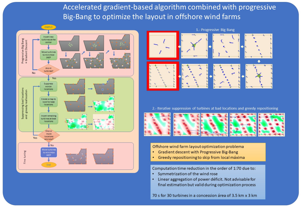
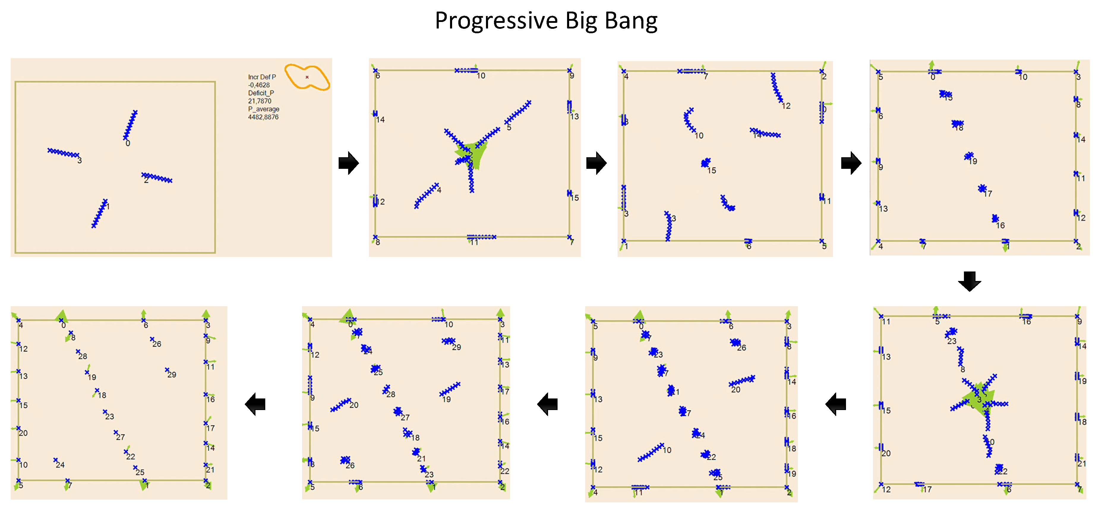
In broad strokes, this problem will be solved by means of a sequence of operations by which layouts with decreasing

U = δ A E P / T

would be obtained. The updating of the successive solutions will be carried out using the gradient method. However, since the optimization function is non-convex, this method must be accompanied by some modification that allows the detection of local optima, and skip to another solution with lower potential. In addition, it will not start from an initial configuration of

n t

turbines, but every certain number of iterations, a set of turbines will be included, allowing each configuration to evolve to occupy the areas with less interactions, typically the corners and the contour. This aspect of the algorithm has been called Progressive Big Bang (PBB).

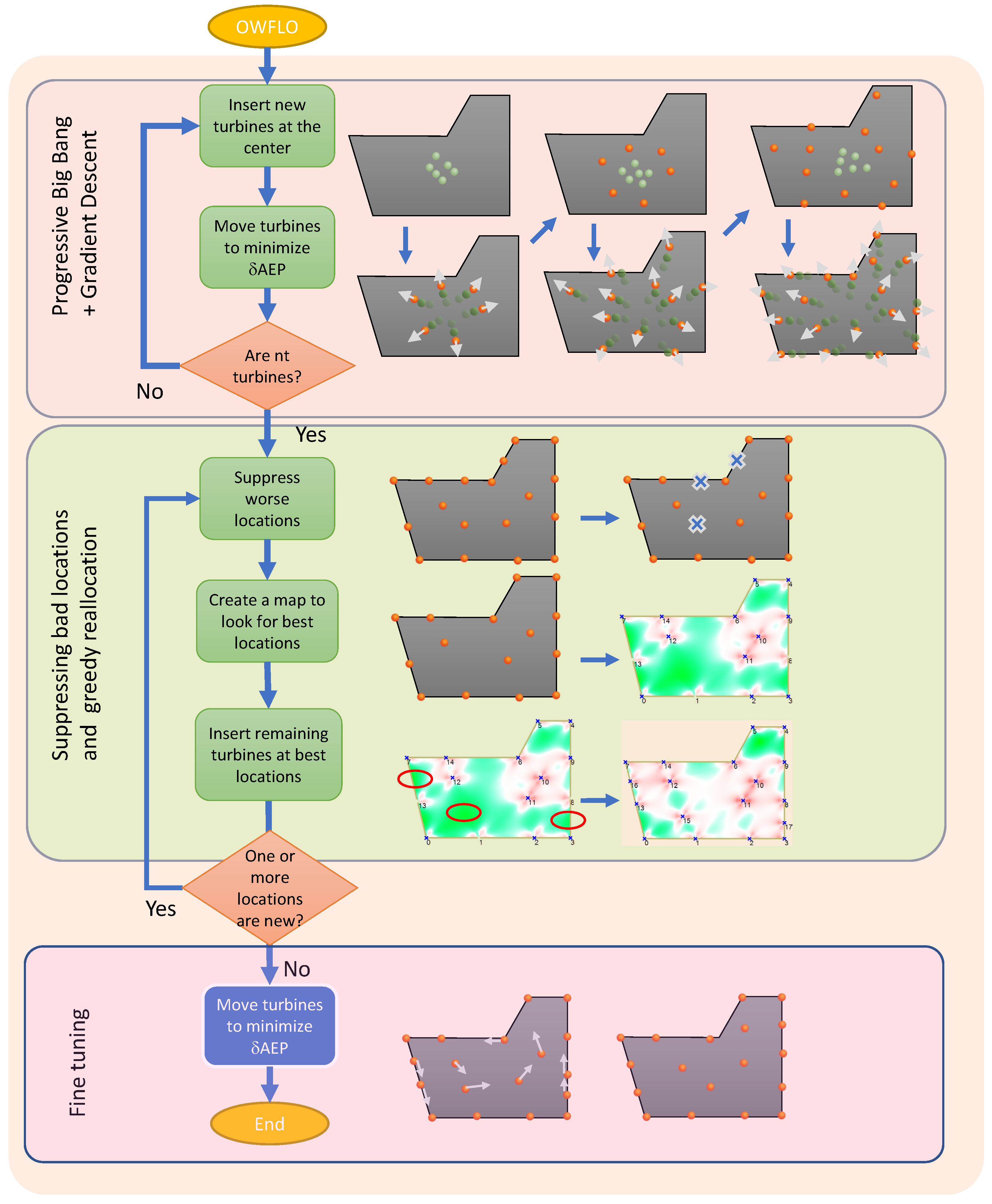
In this work, this combined method will be used and compared to a modified genetic algorithm. The proposed method is shown in Figure 3 and consists of the following:

Progressive Big-Bang. Figure 4 show different frames of this process.
- Initial placement of turbines in the central area of the CA. In Figure 3 six turbines are included at every batch
- Expansion of the turbines using the gradient method
- Repeat the previous steps until $n t$ turbines are included
Greedy Repositioning. Its details will be explained in subsection 5.4.

4.

Identification and suppression of turbines in areas with high U (i.e. high energy deficit or average power deficit)

5.

Creation of a map to detect positions with less U to locate the suppressed turbines there

6.

Repeat steps 4-5 until no new optimal positions are obtained.
Final Tuning

7.

Use the gradient method again to tune the layout.

The gradient-descent method is present in step 2 and step 6, and their details will be explained below.

5.2. Gradient method

Among the variants of the gradient method, one of the most used for solving large-scale nonlinear optimization problems is the conjugate gradient method, introduced for nonlinear systems by Fletcher and Reeves in the 60s. For linear systems, it is faster than the basic gradient descent method. However, in the case under study, obtaining an analytical expression for the function to be minimized (

A E P

), as in [9,10,11] will increase the computation time. This time is even larger if the inverse of (28) or its Hessian is required to obtain a correct value of the learning rate to meet the inequalities of the strong Wolfe conditions [25].

Instead, the basic gradient descent method will be used. With regard to the learning rate (or step size), at Step 2, it is simply calculated as a function of the change rate of

\bar{P}

(see Figure 5). At step 7, the learning rate is greatly reduced to allow a fine tuning.

Traditionally, the GD method is based on the calculation of the gradient of an objective function, in this case

U = δ A E P / T

, which depends on the positions of the

n t

turbines, giving rise to a gradient vector of

2 n t

components.

\begin{matrix} \nabla U = {[\frac{\partial U}{\partial q_{1}} \dots \frac{\partial U}{\partial q_{2 n t}}]}^{T} with q_{2 j - 1} = x_{j} and q_{2 j} = y_{j} \end{matrix}

(29)

5.2.1. $δ A E P$ as a potential energy

It was seen in Section 4 that, when an interaction exists due to multiple wakes on the same downwind turbine, several aggregation methods can be used to estimate the speed deficit suffered by the air stream passing through the downwind turbine. With an adequate modelling of wind conditions, the quadratic and linear methods (QAVD and LAVD) gave results comparable to those ones obtained directly from SCADA systems. Another method with similar results to LAVD is LAPD; that is, the power deficit generated by a downwind turbine affected by several turbines is the sum of the power deficits calculated considering each interaction separately. Despite a deviation higher than QAVD or LAVD, the proposed method, LAPD, gives rise to a similar power deficit map, and therefore a similar distribution of gradients, as shown by comparing maps a) and c) of Figure 2.

In addition, it will be seen that, by using LAPD, the optimization problem of

2 n t

variables shown in (28) is reduced to optimizing

n t

problems of two variables. Indeed, taking partial derivatives with respect to, e.g., component

x_{i}

, it yields

\frac{\partial U}{\partial x_{i}} = \frac{\partial \sum_{k} δ {\bar{P}}_{k}}{\partial x_{i}} = \sum_{k} \frac{\partial \sum_{j \neq k} δ {\bar{P}}_{j \to k}}{\partial x_{i}} = \sum_{k} \sum_{j \neq k} \frac{\partial δ {\bar{P}}_{j \to k}}{\partial x_{i}}

(30)

and since

\begin{matrix} j \neq i \\ k \neq i \end{matrix}\} \Rightarrow \frac{\partial δ {\bar{P}}_{j \to k}}{\partial x_{i}} = 0

(31)

it yields

\begin{matrix} \frac{\partial U}{\partial x_{i}} = \sum_{j \neq i} \frac{\partial δ {\bar{P}}_{j \to i}}{\partial x_{i}} \\ \frac{\partial U}{\partial y_{i}} = \sum_{j \neq i} \frac{\partial δ {\bar{P}}_{j \to i}}{\partial y_{i}} \end{matrix}

(32)

{\hat{e}}_{x}

{\hat{e}}_{y}

are the unitary Cartesian vectors, then we can define

\nabla^{i} \cdot \equiv \frac{\partial \cdot}{x_{i}} {\hat{e}}_{x} + \frac{\partial \cdot}{y_{i}} {\hat{e}}_{y}

(33)

and (32) turns into

\nabla^{i} U = \sum_{j \neq i} \nabla^{i} δ {\bar{P}}_{j \to i}

(34)

From (26), it also results

\nabla^{i} δ {\bar{P}}_{i} = \sum_{j \neq i} \nabla^{i} δ {\bar{P}}_{j \to i} \Rightarrow \nabla^{i} U = \nabla^{i} δ {\bar{P}}_{i} .

(35)

Since

\nabla^{i} U

is parallel to

\nabla^{i} δ {\bar{P}}_{i}

(in fact equal), by moving a turbine along

- \nabla^{i} δ {\bar{P}}_{i}

, the maximum decrease of U will be reached. This assert decouples and simplifies the process, to turn the problem of optimizing in

R^{2 n t}

into

n t

problems in

R^{2}

. In order to obtain the gradient of the power deficit

{\bar{P}}_{i \to j}

, it is faster to firstly calculate the gradient in polar coordinates,

\nabla = \frac{\partial}{\partial r} {\hat{e}}_{r} + \frac{1}{r} \frac{\partial}{\partial θ} {\hat{e}}_{θ} \Rightarrow \nabla = \frac{\partial}{\partial r} (cos θ {\hat{e}}_{x} + sin θ {\hat{e}}_{y}) + \frac{1}{r} \frac{\partial}{\partial θ} (- sin θ {\hat{e}}_{x} + cos θ {\hat{e}}_{y})

(36)

where r and

θ

are respectively the radial and angular components which corresponds to the separation between turbines and orientation between them, and

{\hat{e}}_{r}

{\hat{e}}_{θ}

are unitary vectors in the radial direction and its perpendicular direction CCW. Therefore

\begin{matrix} \frac{\partial δ {\bar{P}}_{i \to j}}{\partial x_{i}} = \frac{\partial δ {\bar{P}}_{i \to j}}{\partial r} cos θ - \frac{1}{r} \frac{\partial δ {\bar{P}}_{i \to j}}{\partial θ} sin θ \\ \frac{\partial δ {\bar{P}}_{i \to j}}{\partial y_{i}} = \frac{\partial δ {\bar{P}}_{i \to j}}{\partial r} sin θ + \frac{1}{r} \frac{\partial δ {\bar{P}}_{i \to j}}{\partial θ} cos θ \end{matrix}

(37)

5.3. Implications of the decoupling

The optimization process to minimize

δ \bar{P}

can be decoupled by using LAPD. This means that, at each iteration, the algorithm can move every turbine i looking for reducing its power deficit

δ {\bar{P}}_{i}

. Performing that for every turbine will result in a overal optimization

\bar{P}

. In addition, any interaction

δ P_{i \to j}

and its gradient components (37) only depends on the distance r between turbines i and j and the orientation

θ

of the segment which links them. Therefore, it can be precalculated offline and accessed in execution time through a 2D look-up table. If a fixed step for the gradient descent method is used, or at least not dependent on the gradient magnitude, the precalculated gradient values can be summed using (34), and the result used to move the turbine.

5.4. Suppressing bad locations and greedy repositioning

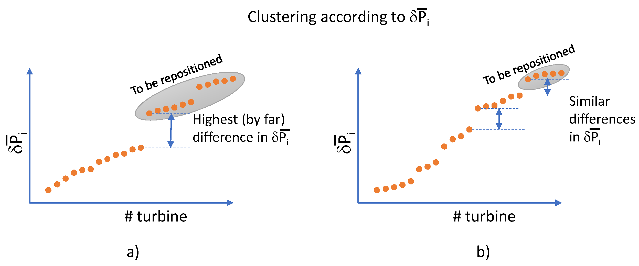
The GD method may be unable to drive a turbine located in the centre of three or four other turbines. This would be a case of local optimum that should be avoided. To this end, after using the gradient method with the

n t

turbines in the CA, a potential map is created that detects which turbines have a much higher potential than others. To achieve this goal, the turbines are ordered according to their potential (

δ {\bar{P}}_{i}

) and the differences between two consecutive turbines are calculated. This allows gathering the turbines and identifying which turbine cluster can be removed.

Figure 6 visualizes the issues that are taken into account to suppress a cluster (and the following ones):

a): The cluster with the largest gap with the previous one is more prone to be suppressed.
b): The suppression of clusters with higher potential (power deficit) is preferred.

It is worth mentioning that this tool is feasible only if the

\bar{P}

evaluation can be performed in a very reduced time. As previously mentioned, by using LAPD, every map (500x428 calculations) takes less than 3s.

Once these turbines located in high potential positions have been eliminated, a potential map is created, the absolute minimum is found, a turbine is placed there and the potential map is re-created. Figure 7 shows several frames of this iterative process.

6. Results

In order to validate the LAPD method to merge multiple wakes, as well as to test the performance of the proposed algorithm, a set of simulations have been launched.

The workbench is a rectangular area of 3500m x 3000m in which 30 turbines must be placed. The wind conditions and the model used are those of Horns Rev I, whose data are shown in Table 2 and Table 3.

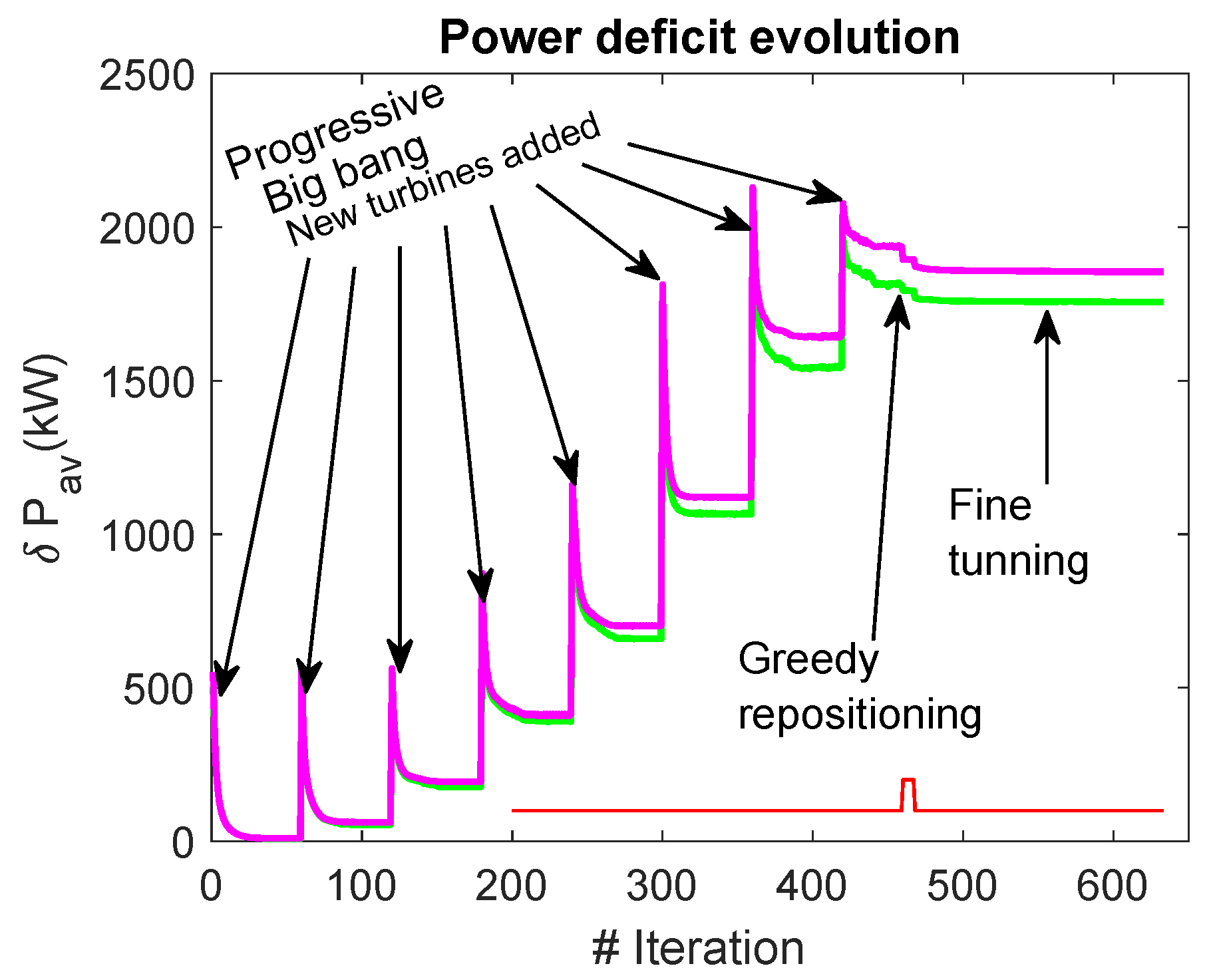
To this end, Figure 8 shows the evolution of the farm deficit as the algorithm progresses. In green, the evolution of the estimated

A E P

by using LAPD is shown, which is the method actually used during the optimization. In magenta, the evolution of the

A E P

estimated using LAVD is shown, which is not used during the optimization, but is included in the graph to check that both aggregation methods present parallel evolutions; therefore it is coherent to think that LAPD can be used during the optimization process in order to minimize losses due to wake effect.

Most of the iterations correspond to the PBB, in which turbines are added in the centre. In the next step, they repel each other due to the strong interactions they suffer, thus reducing their own potential (power deficit) and that of the farm. The repulsion mechanism seeking the minimization of the potential presents an analogy with the electrostatic force of repulsion, which turns out to be the potential gradient. Therefore, it seems appropriate to use the gradient as a force that determines the movement of the particles/turbines in order to minimize their potential.

Once all the turbines have been located, in order to detect and reallocate the turbines that can cause local optima, a Greedy repositioning mechanism is used to suppress the turbines that cause the greatest power deficit and creates a potential map. Then, it tracks the map searching for the optimal location and places a turbine at that particular place. Then, a potential map is recreated to place a new turbine. The process repeats till the best new locations are the same as the previously suppressed one, which indicates that no further improvement can be obtained.

Finally, a search is run again using the GD method with a smaller learning rate, to adjust the final maximum. It should be said that this last process does not lead to a significant improvement in the estimated U.

In order to compare the proposed algorithm with a traditional one, a genetic algorithm has been programmed and launched, whose fitness is

\bar{P}

. It is programmed in a similiar way to the binary GA explained in [26], and start from a grid of

n r

rows and

n c

columns. There were, therefore,

n r \times n c

possible positions to locate the

n t

turbines, and

n r \times n c

binary chromosomes indicating whether a cell was occupied by a turbine or not. However, in this new case, chromosomes are not binary number, but discrete values. Each of the

n t

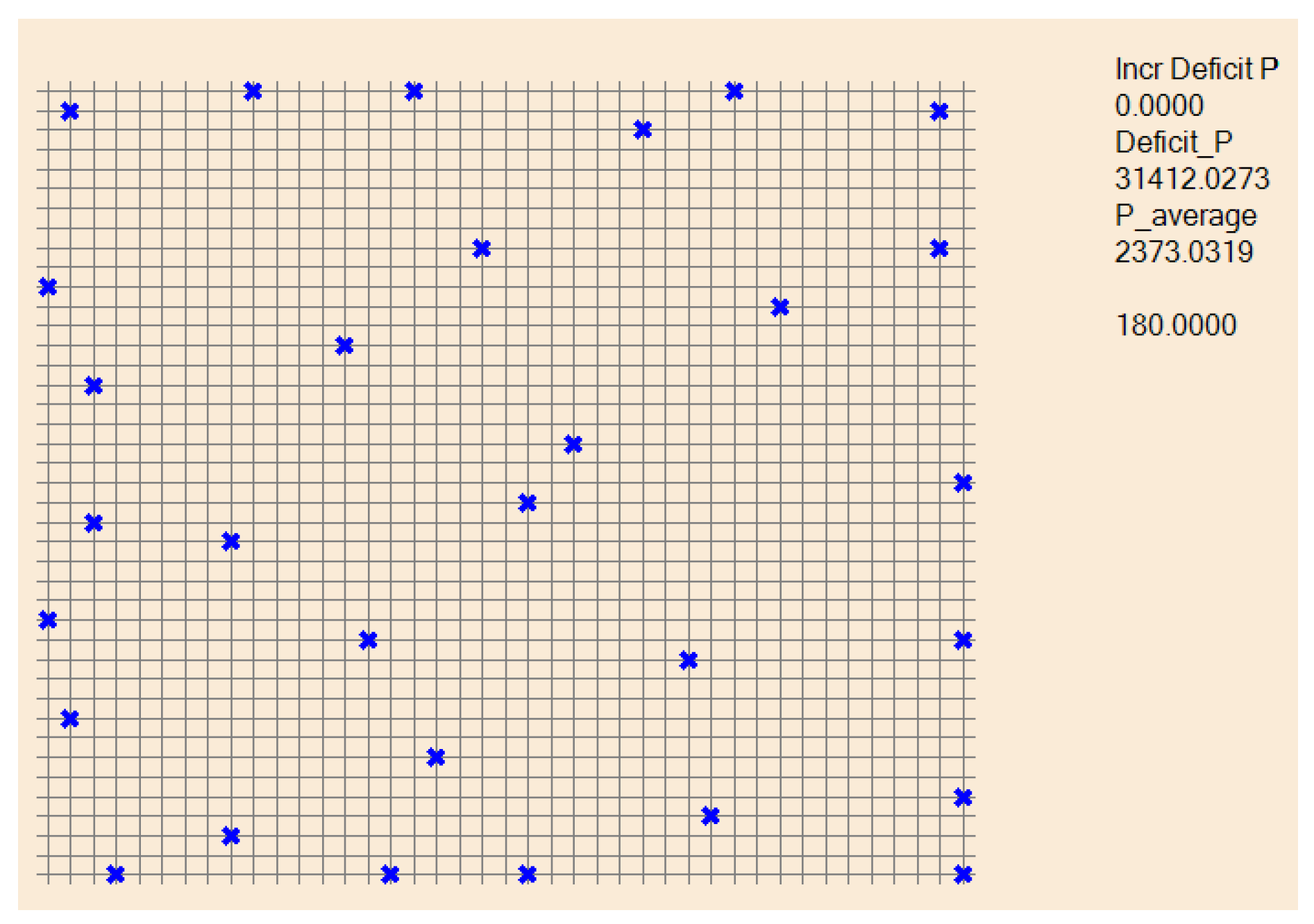
chromosomes corresponds to a turbine and is represented by the value of the column and row where the turbine is located. Figure 9 shows an example of a possible solution as given by this algorithm. Its configuration parameters are: offspring size obtained from crossover, 25%; offspring size obtained from mutation, 25%; individual disregarded when obtaining the offspring, 20%; population size, 200 individuals; maximum number of generations, 3000; maximum number of stagnant generations, 300.

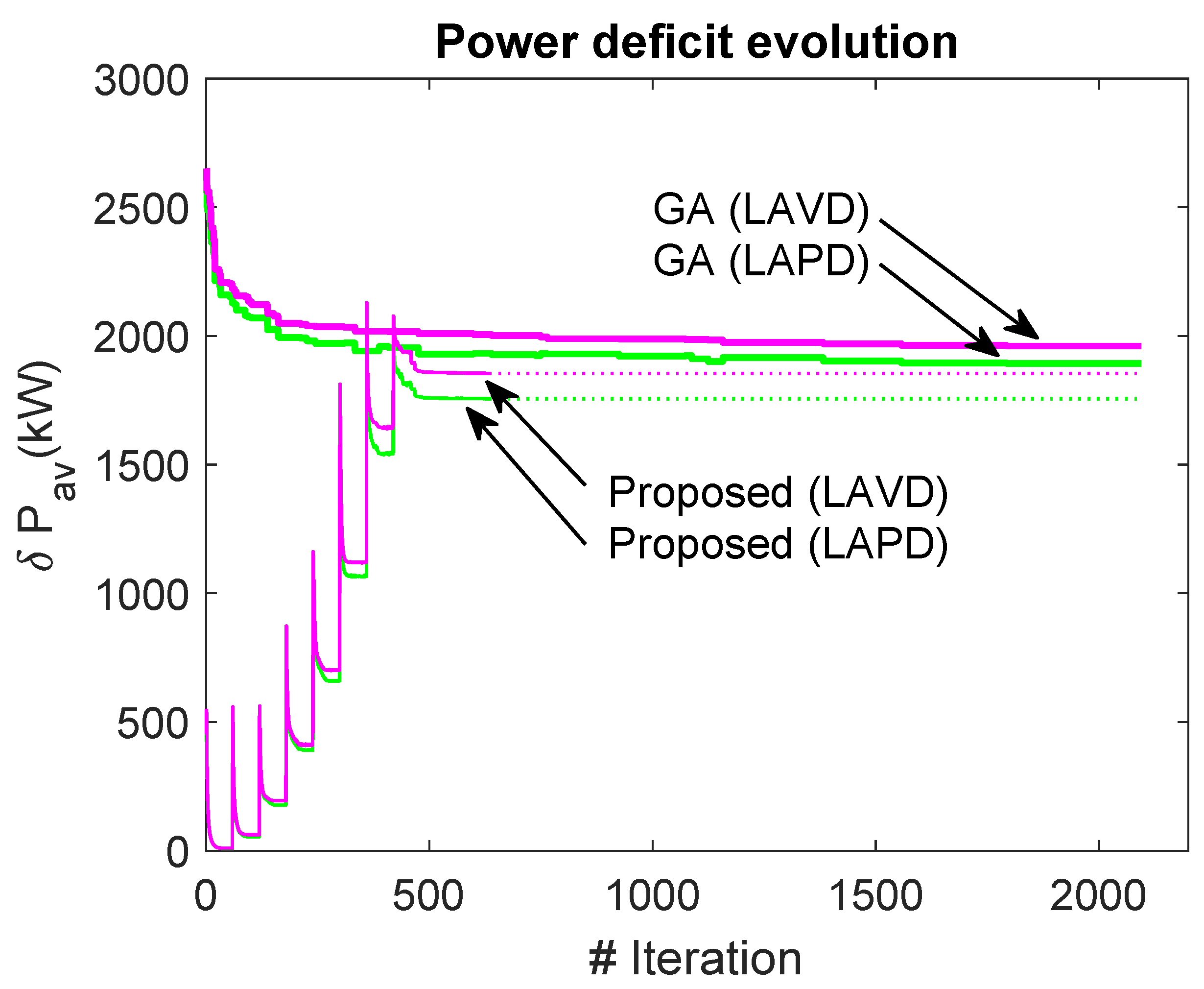
The fitness (

\bar{P}

) evolution is depicted with thick line in Figure 10, and is compared to the result obtained by the proposed algorithm (Progressive Big Bang + Gradient Descent + Greedy Repositioning), in thin line. For both method, the average power is presented, on one hand calculated with LAVD (magenta) and on the second hand calculated with LAPD (green). As seen, also for the GA, both estimates present parallel evolutions, and, irrespective of which method can be used to obtain a final accurate estimation of

A E P

, the LAPD method can be used to perform faster searches.

A set of twenty experiments have been performed to compare both algorithms. In order to speed-up the searches, the LAPD method has been used to estimate

\bar{P}

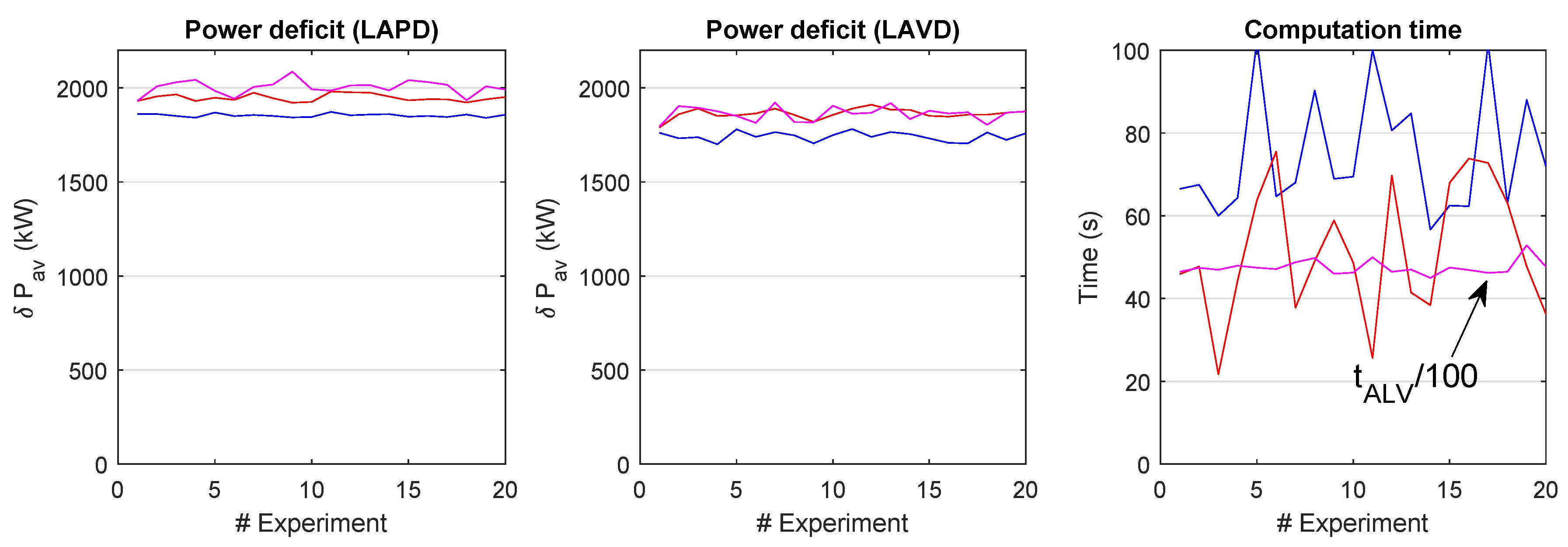
, and also for the potential maps and gradients. A third set of experiments have been launched using GA implementing the LAVD estimation as fitness. It will be named as GA-LAVD and corresponds to a traditional procedure. Figure 11 represents the results: blue for GD-LAPD, red for GA-LAPD, and magenta for the traditional GA-LAVD.

Table 6 summarizes the obtained results. Second column is the deficit obtained implementing LAVD, more accurate than LAPD, and it was the objective function of GA-LAVD. Third column shows the computation time. For the algorithms developed using the LAPD estimations, the twenty experiments were completed in less than 25 minutes. Comparing the last two rows, it can be seen that the performance (in terms of objective function) is not deteriorated if the GA uses the LAPD method instead of the traditional LAVD one (1861 for GA-LAVD and 1862 for GA-LAPD) for the objective function. With the proposed algorithm, and using LAPD for the objective function (GD-LAPD), the power deficit is reduced to 1742, i.e. 6.9% of improvement for the proposed method, with regard to any of the GA. These results confirm that LAPD can be used as objective function during the search process, and the optimum solution obtained using this aggregation method will be the same optimum solution that using LAVD as aggregation method.

In the proposed method (GD-LAPD), the reduction in time is around 1:65 with respect to GA-LAVD, and around 1.5 worse than GA-LAPD.

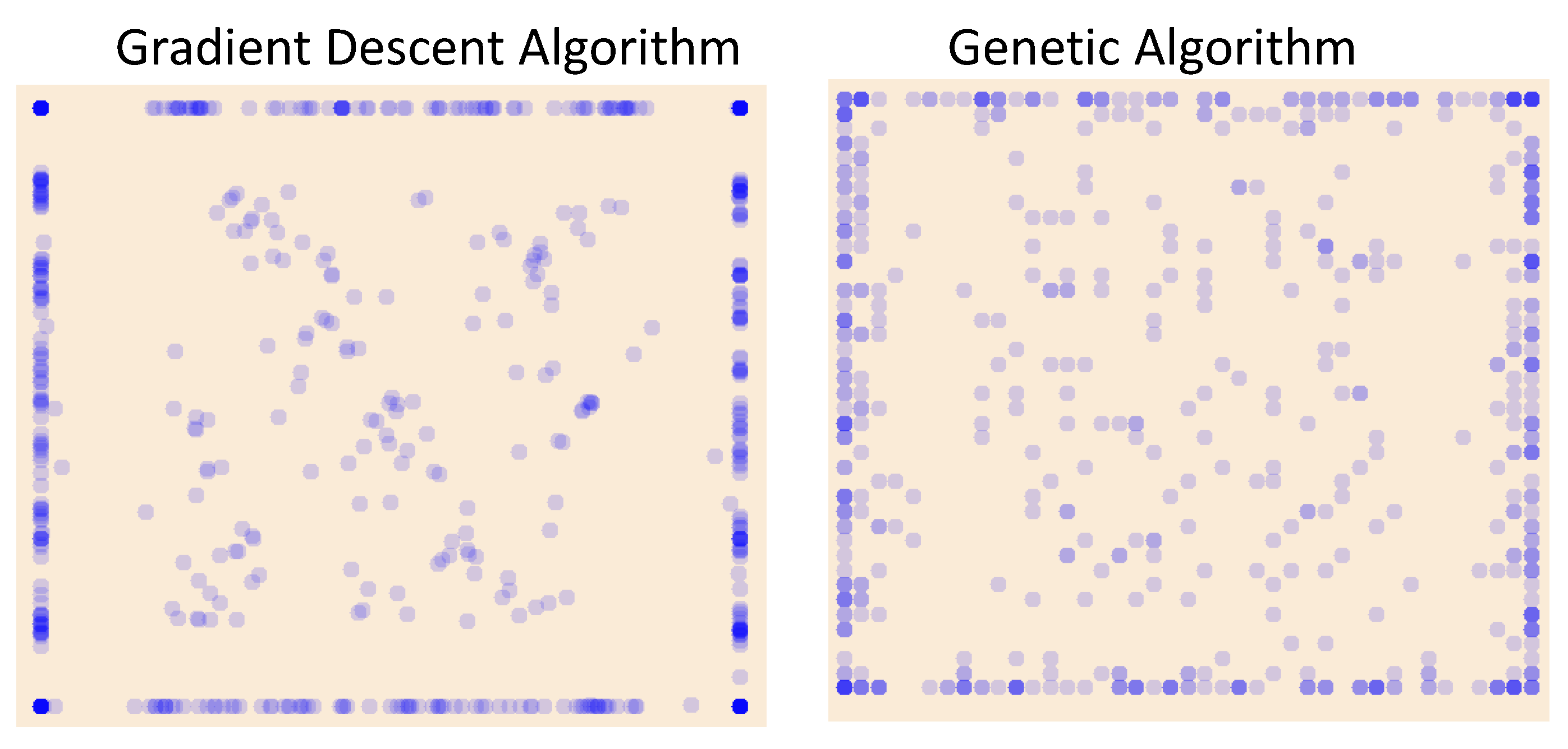
Finally, Figure 12 represents the turbine locations for the optimum solutions, both for the set of GD experiments and for the set of GA experiments. In both cases, the turbines are preferentially located at the concession area contour in order to maximize the distances between them. However, the inner turbines are more scattered when the GA is used. In the GD algorithm, the vertices are more likely to be occupied, and certain trend is observed to dispose the inner turbines in a shape similar to that of Figure 7.

As a result, it has been seen that the proposed algorithm obtains better solutions that a traditional GA-based one. The required computation time is drastically reduced in both cases if, during the search, the LAPD method is used to evaluate the power deficits. If, as in the case of GA, only the power deficit is estimated, this time reduction is around 1:150. If also gradients are required, it reaches 1:600.

7. Discussion

One of the problems attached to the gradient method is the possibility of reaching local maximums that prevent the achievement of a global optimum. By starting through a progressive big-bang, the turbines are repelled towards the periphery, which is usually optimal for wide-spreading purposes. In an intermediate stage, after a first optimization with the possibility of falling into local maximums, the algorithm suppressed the turbines that eventually give rise to local maxima, and new positions are sought for them. Finally, another gradient-based search is performed to finally tune the result.

The presented work uses a new aggregation method, LAPD, to calculate the power deficit and the gradient direction. With this, the problem is partially linearized, and an analogy can be found with the repulsion electrostatic forces. According to this analogy,

Turbine i→ electrostatic charge i
Power deficit at turbine i→ electrostatic potential energy of charge i
Overall power deficit → electrostatic potential energy of the set of charges
Gradient of power deficit at location (x,y) → electric field energy at location (x,y). It should be noted that the electric field in this analogy would not be isotropic, but similar to a wind rose, accounting for the fact that it will be a higher repulsion in the directions where the wind rose is more prominent.

As it is known, the electric field

\vec{E_{e l}}

and the electrical potential

U_{e l}

are related through

\vec{E_{e l}} = - \nabla U_{e l}

, and hence the particle will move along the directions of

\vec{E_{e l}}

in order to minimize their own potential energy and also the overall one. This is possible due to the linear character of electrostatic potential. The linearization obtained implementing LAPD will allow the algorithm to behave in a similar way, moving the turbines in the direction of power deficit gradient for each turbine, in order to obtain an overal optimization.

From a purely mathematical point of view, this method does not guarantee the achievement of the global optimum. Actually, given the uncertainties in the modelling of the system, mainly due to inaccurate wind condition forecasting and imprecise wake modelling, a deviation in the assumed conditions or models can lead to unrealistic objective function values. Therefore, an exhaustive search for the global optimum is not worthy if its neighbourhood of monotonicity is very small. In this sense, flatter local optima are preferable, even though they may be of lower value.

Another problem cited in the bibliography, which appears for large farms, is the high computing time. Throughout this work, three tools have been provided to simplify and accelerate the calculation of the objective function and its gradient, thanks to them the search for the optimum is carried out in a much shorter time compared to previous works. These tools are: point symmetry, LAPD method and look-up tables. This last tool is possible due to the linearization achieved with LAPD.

Many works deal with land-use constrains as concerns that are difficult to handle. In this paper, this issue does not entail a significant problem and it is solved in a natural and geometrical way by limiting the movement targets to the concession zone contour.

Author Contributions

Conceptualization, Angel Gonzalez-Rodriguez; Data curation, José Vicente Muñoz Díez; Formal analysis, Angel Gonzalez-Rodriguez and Juan Roldan-Fernandez; Funding acquisition, Juan Roldan-Fernandez; Investigation, Angel Gonzalez-Rodriguez and Juan Roldan-Fernandez; Methodology, Angel Gonzalez-Rodriguez and Juan Roldan-Fernandez; Project administration, Juan Roldan-Fernandez; Resources, Juan Roldan-Fernandez; Software, Angel Gonzalez-Rodriguez and José Vicente Muñoz Díez; Supervision, Angel Gonzalez-Rodriguez; Validation, Angel Gonzalez-Rodriguez and Juan Roldan-Fernandez; Visualization, José Vicente Muñoz Díez; Writing – original draft, Angel Gonzalez-Rodriguez; Writing – review and editing, José Vicente Muñoz Díez.

Funding

This work has been supported by the Andalusian Government under grant PROYEXCEL_00588

Institutional Review Board Statement

Not applicable.

Informed Consent Statement

Not applicable.

Conflicts of Interest

The authors declare no conflict of interest.

Abbreviations

The following abbreviations are used in this manuscript:

AEP	Annual energy production
CA	Concession area
$δ \cdot$	deficit of ·
GA	Genetic algorithm
GD	Gradient descent
QAVD	Linear aggregation of velocity
LAPD	Linear aggregation of power deficit
FDAG	Finite-difference approximation of gradients
OWF	Offshore wind farm
OWFLOP	Offshore wind farm layout optimization problem
$\bar{P}$	Average farm power
PBB	Progressive Big-Bang
PS	Point symmetry
LAVD	Quadratic aggregation of velocity
U	Potential energy, analogous to energy deficit or average power deficit

References

Elkinton, C.; Manwell, J.; Mcgowan, J. Algorithms for Offshore Wind Farm Layout Optimization. Wind Engineering 2008, 32, 67–84. [CrossRef]
Yang, K.; Kwak, G.; Cho, K.; Huh, J. Wind farm layout optimization for wake effect uniformity. Energy 2019, 183, 983–995. [CrossRef]
Cazzaro, D.; Pisinger, D. Variable neighborhood search for large offshore wind farm layout optimization. Computers and Operations Research 2022, 138, 105588. [CrossRef]
Herbert-Acero, J.F.; Probst, O.; Réthoré, P.E.; Larsen, G.C.; Castillo-Villar, K.K. A Review of Methodological Approaches for the Design and Optimization of Wind Farms. Energies 2014, 7, 6930–7016. [CrossRef]
Hou, P.; Zhu, J.; MA, K.; Yang, G.; Hu, W.; Chen, Z. A review of offshore wind farm layout optimization and electrical system design methods. Journal of Modern Power Systems and Clean Energy 2019, 7, 975–986. [CrossRef]
Cinar, A.C. A review of 10 × 10 and 20 × 20 grid-type wind turbine placement problems solving by metaheuristics. Environmental Science and Pollution Research 2023, 30, 11359–11377. [CrossRef]
Croonenbroeck, C.; Hennecke, D. A comparison of optimizers in a unified standard for optimization on wind farm layout optimization. Energy 2021, 216, 119244. [CrossRef]
Pérez, B.; Mínguez, R.; Guanche, R. Offshore wind farm layout optimization using mathematical programming techniques. Renewable Energy 2013, 53, 389–399. [CrossRef]
Park, J.; Law, K.H. Layout optimization for maximizing wind farm power production using sequential convex programming. Applied Energy 2015, 151, 320–334. [CrossRef]
Guirguis, D.; Romero, D.A.; Amon, C.H. Toward efficient optimization of wind farm layouts: Utilizing exact gradient information. Applied Energy 2016, 179, 110–123. [CrossRef]
Guirguis, D.; Romero, D.A.; Amon, C.H. Gradient-based multidisciplinary design of wind farms with continuous-variable formulations. Applied Energy 2017, 197, 279–291. [CrossRef]
Risco, J.; Rodrigues¹, R.; Frederiksen, M.; Quick, J.; Pedersen, M.; Réthoré, P.E. Gradient-based Wind Farm Layout Optimization With Inclusion And Exclusion Zones. Wind Energy Science 2023. [CrossRef]
Yamani Douzi Sorkhabi, S.; Romero, D.A.; Beck, J.C.; Amon, C.H. Constrained multi-objective wind farm layout optimization: Novel constraint handling approach based on constraint programming. Renewable Energy 2018, 126, 341–353. [CrossRef]
King, R.N.; Dykes, K.; Graf, P.; Hamlington, P.E. Optimization of wind plant layouts using an adjoint approach. Wind Energy Science 2017, 2, 115–131. [CrossRef]
Gonzalez-Rodriguez, A.G.; Payan, M.B.; Santos, J.R.; Gonzalez, J.S. Optimization of regular offshore wind-power plants using a non-discrete evolutionary algorithm. AIMS Energy 2017, 5, 173–192. [CrossRef]
Mittal, P.; Kulkarni, K.; Mitra, K. A novel hybrid optimization methodology to optimize the total number and placement of wind turbines. Renewable Energy 2016, 86, 133–147. [CrossRef]
Quick, J.; Réthoré, P.E.; Pedersen, M.; Rodrigues¹, R. Stochastic Gradient Descent for Wind Farm Optimization. Wind Energy Science 2022, pp. 1235–1250. [CrossRef]
Gonzalez-Rodriguez, A.G.; Serrano-González, J.; Burgos-Payán, M.; Riquelme-Santos, J.M. Realistic Optimization of Parallelogram-Shaped Offshore Wind Farms Considering Continuously Distributed Wind Resources. Energies 2021, 14. [CrossRef]
Shao, Z.; Wu, Y.; Li, L.; Han, S.; Liu, Y. Multiple wind turbine wakes modeling considering the faster wake recovery in overlapped wakes. Energies 2019, 12. [CrossRef]
Peña, A.; Schaldemose Hansen, K.; Ott, S.; van der Laan, M.P. On wake modeling, wind-farm gradients, and AEP predictions at the Anholt wind farm. Wind Energy Science 2018, 3, 191–202. [CrossRef]
Ørsted. Offshore Wind Measurement and Operational Data. https://orsted.com/en/what-we-do/renewable-energy-solutions/offshore-wind/offshore-wind-data#offshore-meteorological-data, accessed on August 2023.
Anholt Offshore Wind Farm reaches milestone. https://orsted.com/en/media/newsroom/news/2014/09/anholt-offshore-wind-farm-reaches-milestone, accessed on August 2023.
Energy Numbers. Capacity factors at Danish offshore wind farms. https://energynumbers.info/capacity-factors-at-danish-offshore-wind-farms, accessed on August 2023.
Energy Numbers. Capacity factors at Danish offshore wind farms (png). https://energynumbers.info/files/anholt1.png, accessed on August 2023.
Nocedal, J.; Wright, S., Conjugate Gradient Methods. In Numerical Optimization; Springer New York: New York, NY, 2006; pp. 101–134. [CrossRef]
González, J.S.; Gonzalez Rodriguez, A.G.; Mora, J.C.; Santos, J.R.; Payan, M.B. Optimization of wind farm turbines layout using an evolutive algorithm. Renewable Energy 2010, 35, 1671–1681. [CrossRef]

Figure 1. Layout for different OWFs: Horns Rev 1, Horns Rev 1 with random displacements, Horns Rev 2 and Anholt.

Figure 2. Map of estimated power deficit assuming a certain distribution of turbines: a) estimation using LAVD according to (23); b) estimation using QAVD according to (24); c) estimation using LAPD according to (25).

Figure 3. Sequence of operations for the OWFLOP.

Figure 4. Progressive Big Bang. Several batches in which four new turbines are included, and following, the GD algorithm operates to find their best locations. The wind energy is depicted at the right-hand corner of first frame.

Figure 5. Learning rate as a function of the change rate of U =

\bar{P}

(

Δ U

)

Figure 5. Learning rate as a function of the change rate of U =

\bar{P}

(

Δ U

)

Figure 6. Sorting and clustering the turbines according to their power deficit. a) For a gap significantly bigger than the remaining ones, turbines after this gap are suppressed. b) If two or more gaps are similar, the cluster with worst locations is suppressed.

Figure 7. Iterative suppression of turbines at bad locations and repositioning where U is minimum.

Figure 8. Proposed Algorithm. Evolution of the overall power deficit along the optimization process. In magenta, the overal power deficit

δ \bar{P}

estimation using LAVD. In green, the

δ \bar{P}

estimation using LAPD. The pulse in red represents the greedy repositioning of turbines.

Figure 8. Proposed Algorithm. Evolution of the overall power deficit along the optimization process. In magenta, the overal power deficit

δ \bar{P}

estimation using LAVD. In green, the

δ \bar{P}

estimation using LAPD. The pulse in red represents the greedy repositioning of turbines.

Figure 9. A solution for the OWFLOP as given by the GA.

Figure 10. Fitness evolution for the GA algorithm, compared to the evolution of the proposed GD. In green, the power deficit

\bar{P}

evolution using LAPD, which is the real fitness used in the GA. In magenta,

\bar{P}

evolution using LAVD.

Figure 10. Fitness evolution for the GA algorithm, compared to the evolution of the proposed GD. In green, the power deficit

\bar{P}

evolution using LAPD, which is the real fitness used in the GA. In magenta,

\bar{P}

evolution using LAVD.

Figure 11. Performance comparison for GD algorithm using LAPD as objective function (blue), GA algorithm using LAPD (red), and GA algorithm using LAVD (magenta). On the left and center, the

\bar{P}

estimation for the optimum solution using LAPD and LAVD, respectively. On the right, required time per experiment. For the GD-ALV, time is divided by 100.

Figure 11. Performance comparison for GD algorithm using LAPD as objective function (blue), GA algorithm using LAPD (red), and GA algorithm using LAVD (magenta). On the left and center, the

\bar{P}

estimation for the optimum solution using LAPD and LAVD, respectively. On the right, required time per experiment. For the GD-ALV, time is divided by 100.

Figure 12. Cumulative representations of the turbine locations for the optimum solution. The darker colours represent more frequent positions.

Table 1. Distribution of wind farm optimization search papers according to the optimization technique

Category	Algorithm	Porcentage of articles	Domain
Heuristic	Genetic algorithm	32.82%	Discrete
	Genetic algorithm	6.56%	Continuous
	Evolutionary algorithm	4.65%	Continuous
	Particle swarm	3.28%	Discrete
	Particle swarm	6.55%	Continuous
	Ant colony optimization	1.64%	Continuous
	Monte Carlo simulation	1.64%	Discrete
	Simulated annealing	4.92%	Continuous
	Harmony search	1.63%	Discrete
	Pattern search	4.92%	Continuous
	Random search	3.28%	Continuous
	Greedy heuristic algorithm	3.28%	Discrete
	Greedy heuristic algorithm	1.64%	Continuous
Mathematical	Mixed integer programming	13.11%	Discrete
programming	Gradient-based optimization	13.11%	Continuous
	Total	61

Table 2. Anholt site and HR1 site. Values for probability, and Weibull parameters (scale factor

W e i b_{A}

and shape factor

W e i b_{K}

) for every sector.

W e i b_{A}

given at 135 m for Anholt and at 62 m for HR1.

Table 2. Anholt site and HR1 site. Values for probability, and Weibull parameters (scale factor

W e i b_{A}

and shape factor

W e i b_{K}

) for every sector.

W e i b_{A}

given at 135 m for Anholt and at 62 m for HR1.

Anholt	N	NNE	NEE	E	EES	ESS	S	SSW	SWW	W	WWN	WNN
freq (%)	2.38	4.78	6.71	8.76	10.08	8.38	9.87	13.03	10.68	13.33	8.12	3.88
$W e i b_{A}$ (m/s)	8.35	8.07	8.51	10.67	11.16	10.32	11.98	12.56	10.76	11.52	10.42	8.43
$W e i b_{K}$	2.13	2.22	2.26	2.22	2.35	2.17	2.14	2.89	2.79	2.30	1.79	2.17
HR1	N	NNE	NEE	E	EES	ESS	S	SSW	SWW	W	WWN	WNN
freq (%)	3.8	4.3	5.5	8.3	8.7	6.7	8.4	10.5	11.4	12.2	13.9	6.1
$W e i b_{A}$ (m/s)	8.71	9.36	9.29	10.27	10.89	10.49	10.94	11.23	11.93	11.94	12.17	10.31
$W e i b_{K}$	2.08	2.22	2.41	2.37	2.51	2.75	2.61	2.51	2.33	2.35	2.58	2.01

Table 3. Power curve for the turbines installed respectively at Horns Rev I, Horns Rev II and Anholt. Speed (first row) in m/s and Power (second to fourth rows) in kW.

Model	3	4	5	6	7	8	9	10	11	12	13	14	15	16	>16
Vestas V80	0	66	154	282	460	696	996	1341	1661	1866	1958	1988	1997	1999	2000
SWT 2.3-93	0	53	163	393	682	1039	1430	1730	2040	2241	2300	2300	2300	2300	2300
SWP 3.6-120	0	161	351	635	1026	1544	2204	2910	3399	3567	3596	3600	3600	3600	3600

Table 4. Comparison of the AEP evaluation without using PS, i.e. through (5), and using PS, i.e. through (9).

OWF	Original expression (5)	Using PS (9)	Difference
Horns Rev 1	82037.48	82037.48	0%
Horns Rev 1 modified	81774.74	81773.84	0.0011%
Horns Rev 2	95010.03	95010.16	-0.000136%
Anholt	107570.90	107566.55	0.004%

Table 5. Comparison of capacity factor (cf) obtained from different ways of aggregation

	Aggregation	$\bar{P}$ (MW)	Availability (97%)	cf ¹	SCADA cf
Anholt	LAVD	190.24	184.53	46.2%	47.7%
	QAVD	203.12	197.03	49.3%
	LAPD	179.42	174.04	43.6%

¹ Anholt capacity is 399.6MW.

Table 6. Performance comparison of the proposed GD algorithm, a GD one (both using LAPD for the

δ \bar{P}

estimation) and a GD algorithm using LAVD for the

δ \bar{P}

estimation.

Table 6. Performance comparison of the proposed GD algorithm, a GD one (both using LAPD for the

δ \bar{P}

estimation) and a GD algorithm using LAVD for the

δ \bar{P}

estimation.

	$δ \bar{P}$ in kW (LAVD)	time in s
GD (LAPD)	1742	74.6
GA (LAPD)	1862	51.5
GA (LAVD)	1861	4751.0

Disclaimer/Publisher’s Note: The statements, opinions and data contained in all publications are solely those of the individual author(s) and contributor(s) and not of MDPI and/or the editor(s). MDPI and/or the editor(s) disclaim responsibility for any injury to people or property resulting from any ideas, methods, instructions or products referred to in the content.

© 2023 by the authors. Licensee MDPI, Basel, Switzerland. This article is an open access article distributed under the terms and conditions of the Creative Commons Attribution (CC BY) license (http://creativecommons.org/licenses/by/4.0/).

Copyright: This open access article is published under a Creative Commons CC BY 4.0 license, which permit the free download, distribution, and reuse, provided that the author and preprint are cited in any reuse.

MDPI Initiatives

Important Links

Choose an area of interest and we will send you notifications of new preprints at your preferred frequency.

Disclaimer

Accelerated gradient-based algorithm combined with progressive Big-Bang to optimize the layout in offshore wind farms

Abstract

1. Introduction

2. Annual energy produced by a wind farm

2.1. Discretizing the calculation of the annual energy produced by a turbine

3. Symmetrization

4. Linearization

5. Method. Optimization using the progressive big bang + gradient + greedy reposition method

5.1. Overall algorithm description

5.2. Gradient method

5.2.1. δ A E P as a potential energy

5.3. Implications of the decoupling

5.4. Suppressing bad locations and greedy repositioning

6. Results

7. Discussion

Author Contributions

Funding

Institutional Review Board Statement

Informed Consent Statement

Conflicts of Interest

Abbreviations

References

MDPI Initiatives

Important Links

Subscribe

5.2.1. $δ A E P$ as a potential energy